Airy's function for a doubly connected region

Item Type text; Thesis-Reproduction (electronic)

Authors Murray, James Edward, 1939-

Publisher The University of Arizona.

Rights Copyright © is held by the author. Digital access to this materialis made possible by the University Libraries, University of Arizona.Further transmission, reproduction or presentation (such aspublic display or performance) of protected items is prohibitedexcept with permission of the author.

Download date 29/04/2018 10:11:34

Link to Item http://hdl.handle.net/10150/318169

AIRY'S FUNCTION FOR A DOUBLY CONNECTED REGION

byJames Edward Murray

A Thesis Submitted to the Faculty of theDEPARTMENT OF CIVIL ENGINEERING

In Partial Fulfillment of the Requirements For the Degree ofMASTER OF SCIENCE

In the Graduate CollegeTHE UNIVERSITY OF ARIZONA

1 9 6 8

STATEMENT BY AUTHORThis thesis has been submitted in partial fulfill­

ment of requirements for an advanced degree at The Uni­versity of Arizona and is deposited in the University Library to be made available to borrowers under rules of the Library.

Brief quotations from this thesis are allowable without special permission, provided that accurate acknowledgment of source is made. Requests for permission for extended quotation from or reproduction of this manuscript in whole or in part may be granted by the head of the Civil Engineering Department or the Dean of the Graduate College when in his -judgment the proposed use of the material is in the interests of scholarship. In all other instances, however, permission must be obtained from the author.

s IGN E

APPROVAL BY THESIS DIRECTOR This thesis has been approved on the date shown below:

_______________ A/is /3Neff Date

Professor of Civil Engineering

ACKNOWLEDGMENT

The author wishes to express his sincere thanks to his thesis advisor, Dr. Richmond C . Neff, for his able guidance in the selection of this thesis topic and for his willing assistance during the preparation of the thesis„ In addition to giving continual guidance, Dr, Neff has also made many helpful suggestions.

The author also wishes to thank his wife, Sharon, for her cooperation and assistance in the preparation of this thesis.

TABLE OF CONTENTSPage

LIST OF ILLUSTRATIONS . . . , . . . . . . . . , , . . vLIST OF TABLES . . „ . . . . ...... . . . * . . ■ . . viABSTRACT ^XLCHAPTER

1 INTRODUCTION . 12 THEORY AND DERIVATIONS FOR THE ANALYSIS . . . ■ 3

Airy9 s Stress Function ........ 4Method of Solution . . . . . . . . . . . . . . 6Boundary Conditions . . . . . . . . . . . . . 8Multiple-Valued Parts of Airy’s

Stress Function , . . . . . . . . . . . . 10Derivation of the Programmable Equations . . . 11

3 ACCURACY OF THE METHOD . . . . . . . . . . . . 20The Numerical Integration . . . . . 23Truncation of the Series . . . . . . . . . . . 26Computer Truncation ............28

4 VERIFICATION OF THE METHOD . . . . . . . . . . 32Closed Form Solutions . . . . . . . . . . . . 33Finite Element Comparison . . . . . . . . . . 37

5 CONCLUSIONS AND FUTURE INVESTIGATIONS . . . . 42REFERENCES @ © © © © ©. . © © © © © . .© . © © © . . . 44

>

iv .

LIST OF ILLUSTRATIONS

Figure Page

1 A Boundary Element with Surface Tractionsand Stresses in Equilibrium . . . . . . . 9

2 A Doubly Connected Region with a BranchCut . . . . . . . . . . . . @ 0 . 0 . . . 12

3 Perforated Square Plate with 100 psi.Uniaxial Load . . . . . . . . . . . . . . 21

4 Upper Right Quadrant of Perforated Square Plate with Fifteen PointsRandomly Selected for Analysis . . . . . 22

5 Submerged Cylinder Filled with Fluid so that the Loading is Symmetricalwith Respect to the X-axis . . . . . . . 34

6 Submerged Cylinder Filled with Fluid so that the loading is Symmetricalwith Respect to the Y-axis . . . . . . . 35

7 Upper Right Quadrant of Perforated Square Plate Divided into 79 FiniteE lent exits . . . . . . . . . . . . . . . . 39

v

LIST OF TABLES

Table

1 Comparison of Results Calculated with Sixteen and Nine Integration Intervals o e e e e e o e e o e f l o o

2 Results Obtained Using 40 and 41 Coordinate Functions

3 Comparison of Results Using Eight and Thirteen Significant Figures . .

4 Verification of the Airy's StressFunction Solution by a Finite Element Solution ...................

Page

. 27

29

31

. 41

vi

ABSTRACT

This thesis presents a series type solution for plane elasticity problems with boundaries defined by doubly connected regions and with the boundary stress tractions known, A complete Airy1s Stress Function as given by J.H. Michell is used in conjunction with a Modi­fied Trefftz Procedure to formulate equations suitable for computer solutions. The Modified Trefftz Procedure is a minimization of the integral around the outer and inner boundaries of the squared error in the gradient of the stress function..

Results of the method are verified by comparisons to closed form solutions of Lame *s Problem and of the submerged cylinder problem. Results are also compared to a finite element solution of the stresses in a square plate with a central hole under uniaxial loading. An error analysis is included which points out the areas of inaccuracy and indicates the significance of the errors.

vii

CHAPTER 1

INTRODUCTION\

The solution of elastic stress distributions for plane elasticity problems has received considerable attention for many years. Until the invention of the digital computer, these solutions were restricted to problems of simple loadings on bodies of classical geo­metric shapes. Since the computer has become available to the analyst, many approximate methods have been devised to solve the more complicated problems.. Practical techniques are usually not available for evaluating the errors inherent to most of these methods, and many of the methods require straight line representations of the geometry of the stressed bodies,

Presented in this thesis is a method which solves a certain class of problems with a discernible degree of accuracy and with no limitations on the boundary shapes. This class of problems is characterized by stressed bodies in the form of doubly connected regions with known boundary tractions.

The method is based on the relationships of Airy1s Stress Function which are derived from equilibrium

1

2considerations. Compatibility is satisfied by proper selection of coordinate functions to represent Airy’s Stress Function, and the boundary conditions are met by applying the Modified Trefftz’s Procedure.

The Modified Trefftz’s Procedure minimizes the squared error of the gradient Of the series representation of the Airy’s Stress Function on the boundaries of the region. This process satisfies the boundary conditions because the gradient of the stress function is directly related to the boundary tractions.

CHAPTER 2

THEORY AND DERIVATIONS FOR THE ANALYSIS

Airy’s Stress Function is a convenient represen­tation of the stresses in plane elastic regions, and Airy1s Function must satisfy the partial differential equation known as the biharmonic equation. The gradient of Airy’s Stress Function is directly related to a boundary traction integral and it is this relationship which provides a means of satisfying the boundary con­ditions.

Each term of the series which is used to approxi­mate Airy’s Stress Function will satisfy the differential equation exactly, and the boundary conditions are met by applying the method of least squares to the gradients of Airy’s Stress Function and the approximate stress function. When an infinite number of terms of the approxi­mate stress function are taken, the boundary conditions are satisfied exactly.

After the relationships invoIving Airy's Stress Function, the approximate stress function, and the boundary tractions have been derived, these relationships will be expanded and manipulated until a programmable set of equations is obtained.

3

Airy’s Stress Function G .B . Airy, the British astronomer, first noted

that the stress components could be represented by a single function, U, as shown in the equation below

crx = d2U/dy2(Ty = d 2U/dx2 2.1Txy = -d2U/dydx

or the equations in polar coordinates are

CT = (l/r)(dU/<dr) + (l/r2)(d2U/de2)<Te = d 2U/dr2Tre = (l/r2)(dU/d6) - (l/r)(d2U/drde)

where (T, (T q- , rj- are normal stresses and t , tx X r e xy reare shearing stresses. The stress function has thus become known as the Airy's Stress Function (the name Airy is used only when body forces are neglected). A necessary condition that Airy's Stress Function satisfy compatibility requirements is that the stress function satisfy the bi harmonic equation (Sokolnikof f, 1956), that is

2where the harmonic operator V is defined by the equation

V 2 = (d2/dx2) > (d2/dy2)

For a doubly connected region, satisfaction of the biharmonic equation is a necessary condition for com­patibility, but this does not necessarily insure single­valued displacements (satisfaction of the biharmonic equation is both a necessary and sufficient condition for single-valued displacements in a simply connected region).A stress function which does satisfy the biharmonic relationship must be investigated and possibly modified to insure compatibility.

Each term of the stress function which is used in the analysis of this thesis does satisfy the biharmonic equation, and the modifications to insure single-valued displacements are presented by Timoshenko and Goodier (1951, p. 117-119). This function is known as Michell's general formulation for a doubly connected region with the origin inside the hole. Michel!fs stress function is presented by Timoshenko and Goodier (1951, p. 116) in a form similar to the following (with alterations to insure compatibility):

Y = A@ + BQr^ + C@ln(r) + G^6 4- GgrGsinG + Ggr6cos6

* AlCr * BlCr3 + Cicr"1 " [d-v)/2] G2rln(r)1 cos6

6+ E ( V V r ” + Bncrn+2 + Cncr-n + Dn6r-«+2) cos(ne)

n=2

♦ E (Ansrn ♦ Bnsrn+2 + + D ^ r ' ^ 2 ) sin(n6)n=2 ns 2.3

where the coefficients of the r and 6 terms are constants and v is Poisson's Ratio.

Method of SolutionThe method is based on Airy's Stress Function and

a function generator which will approximate the stress function. Michell's Formulation is used as the function generator in this analysis and will be represented hereafter in the abbreviated form

YN = E Cnfn 2.4n=lin which, N is the number of terms in the approximate stress function, the Cn are constants, and the f are functions of position. The quantities fn are commonly referred to as coordinate functions.

The method of least squares is used to minimize the error of the gradient of the stress function over the boundary of the region. So the error is given by the equation

E = 1/2 ® \ v u - VYN) - ( W - VYN)ds 2.5

where ds is a differential arc length, the integration is performed along the boundaries enclosing the region by means of a branch cut, and V is the del operator defined (in rectangular coordinates) by the equation

? = i (d/dx) + j (d/dy)

in which i and j are unit vectors in the directions of the coordinate axes. The quantity VU is a function of the surface tractions and its determination is presented in the next section.

After evaluating the cyclic integral, the error, E, will simply be a function of the constants, C^. By taking the partial derivatives of the error with respect to each of the N constants and setting the partial derivatives equal to zero, the constants which minimize the error may be obtained. That is, the equations

dE/dC^ = 0 2.6

are a set of simultaneous equations the solution of which will give minimum error for the selected.

Equations 2.5 and 2.6 are essentially the same as those used to define Trefftz's Method, with the exception that in Trefftz's Method (Fox 1954, p. 200- 202) the integral is performed over the area of the region. Therefore, the method may be referred to as the Modified Trefftz's Method.

8Boundary Conditions

A few of the essential relationships involving the stress function will now be developed. The develope- ment is based on the work of Allen (1954, p. 108). An illustration of an infinitesimal boundary element under the influence of surface tractions (Fig. 1) is included to facilitate the developement. The symbols which have not yet appeared are defined as follows:

C - boundary curve.T - vector of boundary tractions, n - unit normal vector. i - unit vector in the x - direction, j - unit vector in the y - direction, r - position vector of the point.(x,n) - angle between the directions of the

axis and the unit normal vector. k - unit vector out of the paper, s - distance along the curve.A- - point designation if approached from above.A+ - point designation if approached from below.

Equilibrating the forces acting on the element in the figure yields

J. =[o^cos(x,n) + Txysin(x,n)] 1 +[crysin(x,n) + Txycos(x,n)] j

cr.A*f

xy

xy

x

Fig. 1. A Boundary Element with Surface Tractions and Stresses in Equilibrium

10Substituting the partial derivatives of the stress function (Eqs. 2.1) for the stresses gives

T = [(d^U/dy^) (dy/ds ) - (d^U/dxdy) ( -dx/ds)J i * [(d^U/dx^) (-dx/ds) - (d^U/dxdy) (dy/ds )j j

which may be reduced to

T = (d/ds)(du/dy) 1 - (d/ds)(du/dx) j 2.7

Now by forming the cross product of both sides of Eq. 2.7 with the unit vector k, the following result is obtained

k X T = (d/ds)(dU/dx) i + (d/ds)(dll/dy) jor

k X T = (d/ds)( VU) 2.8

The integral relationship.

Vu = VuA ♦ f [d( U)/ds]ds

along with Eq. 2.8 leads to

vu = VUA + J (kXT)ds 2.9

where is the gradient of the stress function evaluatedat the point A.

Multiple-Valued Parts of Airy's Stress FunctionTo determine the discontinuity in ^U, the contour

integral is performed with the result

in which the cyclic integral along the curve, C, is initiated at point A- and closed on point A+. Equation2.10 will be used later to evaluate two coefficients involved in the multiple-valued parts of The righthand side of the equation represents the resultant of the boundary tractions on the closed curve.

It can be shown in a similar manner that the discontinuity in Airy's Stress Function is

where r is the position vector of the point A. Equation2.11 is used later to evaluate one of the coefficients in Y^. The right hand side of this equation represents the moment of the boundary tractions about the point A.

some of the concepts of the derivation. The region, R, represents a doubly connected region with boundarys defined by the curves Co and . Integrations along the boundarys of the region and enclosing the region may be made by means of the branch cut. In this type integration the region is always to the left of the advancing integra-

2 . 1 1

o

Derivation of the Programmable Equations Figure 2 is presented as an aid in visualizing

12

B+

BranchCut

Fig. 2. A Doubly Connected Region with aBranch Cut

13For convenience in the derivation, some equations

from previous sections are repeated below:N

YN ~ ^ Cnfn 2.4n=l

£E = 1/2 ® (VU - VYn).(VU - 7YN)ds 2.5

dE/dCj^ = 0 2.6

L9u = VU,_ * I (kXT)ds 2.9

Substituting for from Eq. 2.4 in Eq. 2.5 yields

E = l / 2 ^ ( V U - ^ C n Vfn ) - ( V U - Z ! CnV f n ) d s

Performing the partial derivatives indicated by Eqs. 2.6 gives

f N _ _J > (^u - C j V f j) -Vfj ds = 0

o r

<p 5 3 C . V f . - V f . d s = < f VV-Vf, V R j = l J J 1 J h

ds

Upon substituting the right side of Eq. 2.9 for VU, this becomes

^ I Z ^ C j V f y V f ^ s = < ^ U a : V f rds

ds 2.12

14Only the constant terms of VY^ are affected by the value of the constant , and these terms do not contributeto the stresses. Therefore, the value of may bearbitrarily assigned, and for convenience this value is chosen to be zero. Equations 2.12 can now be written

fAW"*' = / R [/A-(1?Xf)ds] - ^ t ds 2.13

The cyclic integral is performed along the boundary curve so as to completely enclose the region (Fig. 2). A logical path for this cyclic integral is

■ f . f a\ f \ [ \ [ aJR J A- VA+ J B- JB+

2.14

Since the Integration from A+ to B- is the negative of the integration from B+ to A-, these integrals cancel and Eq. 2.14 reduces to

B+

orJ r va- J b-

(£=<£+<£J r J cq J c t

2.15

The form of the left side of Eqs. 2.13 is readily integrable by numerical procedures. The same is true for the right side of the equation once the bracketed term has been evaluated. Integration along the path from A- to A+ presents no problem. This is not so for the

15integration from B- to B+ because then the bracketed term takes the form

Lvu = 9Ug_ ♦ I (kXT)ds 2.16

and the value of may not be arbitrarily assigned.The value of must correspond to the integral relation,

f B -VUB- = VUM 4- I (kXT)ds 2.17

J A+

Now the boundary tractions along the horizontal branch cut are represented in component form by

T = rxyT +CTyj 2.18

Replacing the stresses by equivalent relations of the stress function (Eqs. 2.1) and substituting this form of Eq. 2.18 into Eq. 2.17 yields

VUB- = ♦ f -k X [ -(d2YN/dydx) j - (d2YN/^x2 ) i]ds J A+

Michel11s formulation of the stress function is used in place of the Airy's Stress Function because it is integrable. After performing the integration, the equation takes the form

B-f (dYN/dy) j + (dYN/dx)i jVUB- = + . ..

A+

= vuA+ + v y n I b . - v y n

or substituting for VYN gives

A*f

16

VU- = VUA+ + E CjVfjB-

NB

Vfj A+

2.19

Using this result in Eq. 2.16 to evaluate the bracketed term on the right side of Eqs. 2.13 makes it nossible to perform the numerical integration along the inside boundary,

There are three constants of Michell’s formulation (Eq. 2.3) which can be evaluated independently of the remaining constants. This is due to the multiple value­dness of the gradient of Michell1s function and of the function itself. The multiple valued terms of the gradient are

v y m = G2 0 j + G3 e t

where indicates gradient multiplevaluedness. The discontinuity is the change in the gradient after one circuit,'that'is

VYM - VYA+ M A-

= ZTTTGgj + G - i ) 2.20

The corresponding relationship for Airy's Stress Function was given in Eq. 2.10 and is repeated here for convenience

VU - VU A+ A

(kXT)ds 2.10

The traction, T, in component form is

¥ = T ix i + T y j

17in which is the x-component and is the y-component. Using this form in Eq. 2.10 and performing the indicated cross product yields

A- = -£(V S)1 2.21vuA - vuA+

Equating the coefficients of i and j in Eqs. 2.20 and 2.21 gives

G2 = II (P T ds277

f T <J c x

and

£G3 "" " I W J C ^ 8

Now the multiple-valued terms of the stress function are

Ym = Gj 6 + G2Qy + Gg8x

and the discontinuity is

= 27T(G^ ♦ G^y^ *f G-^x^)ym A—where x , y are the coordinates of the point A. Equa- A Ating this to the discontinuity of the Airy's Stress Function (Eq. 2.11) yields

G1 = ^ J c(?A - ? >-<*XT)ds - C ^ A ' G3xA

An integration along the outside boundary has been in­dicated but the integration could just as well be performed

along the Inside boundary. All the terms of the gradient of Michell's formulation which are affected by , Gg, and Gg will be represented by the symbol

All the relationships necessary for programming have been derived. The next step is to combine all the equations into one programmable form. First, the per­tinent equations are repeated as follows:

<£=<£+(£J r J co Jc^

(k X T)ds •Vf1ds

vu = vu X T)ds

A+

2.13

2.15

2.16

2.19

Now combining these results gives

This formulation represents N simultaneous equations inthe variables Cj. The N equations are found by giving the index, i, the values 1, 2, ••• N. Although the equations seem quite formidable, their solution is readily obtained on the digital computer.

CHAPTER 3

ACCURACY OF THE METHOD

The three sources of error involved in the calculations of the method are: (1) the approximations of the numerical integrations, (2) the truncation of the stress function, that is, the use of only a finite .number, N, of the coordinate functions, and (3) the truncation of significant figures in the computer cal­culations .

As a means of evaluating the significance of the errors, various modes of solution have been made on the uniaxially loaded three inch square plate with a one inch central hole (perforated plate). The loaded plate is shown in Fig. 3 where the uniform compressive load is 100 psi. In order to compact the resulting data ■and retain a relatively complete analysis of the entire plate, the results at fifteen randomly selected points in the upper right quadrant of the plate (Fig. 4) are used for the error evaluation. Only results from one quadrant are needed because the geometry and the loading are symmetrical to both the x and y axes.

20

21

Fig. 3. Perforated Square Plate with 100 psi.Uniaxial Load

22

14

Point Y-Coordlnate X-CoordinateNo. (inches) (inches)

1 .354 .3542 .090 .5683 .568 .0904 .397 .5465 .601 .3066 .790 .1257 .927 .3018 .789 .5739 .975 .000

10 .192 1.21011 .8 66 .86612 1.210 .19213 .250 1.50014 1.000 1.25015 1.500 1.125

Fig. 4. Upper Right Quadrant of Perforated Square Plate with Fifteen Points Randomly Selected for Analysis

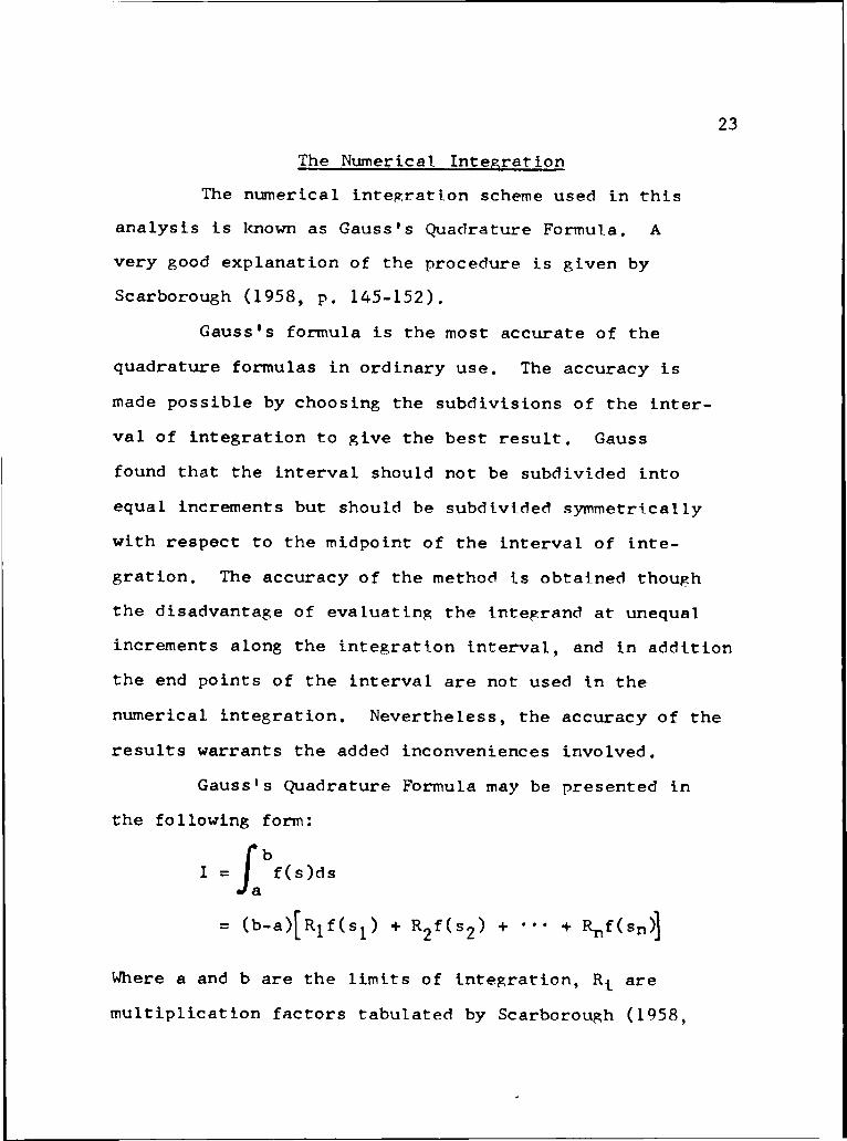
23The Numerical Integration

The numerical integration scheme used in this analysis is known as Gauss's Quadrature Formula. A very good explanation of the procedure is given by Scarborough (1958, p. 145-152).

Gauss's formula is the most accurate of the quadrature formulas in ordinary use. The accuracy is made possible by choosing the subdivisions of the inter­val of integration to give the best result. Gauss found that the interval should not be subdivided into equal increments but should be subdivided symmetrically with respect to the midpoint of the interval of inte­gration. The accuracy of the method is obtained though the disadvantage of evaluating the integrand at unequal increments along the integration interval, and in addition the end points of the interval are not used in the numerical integration. Nevertheless, the accuracy of the results warrants the added inconveniences involved.

Gauss's Quadrature Formula may be presented in the following form:f b

1 = 1 f(s)ds J a

= (b-a)[R1f (sj) + R2f (s2) + ' ' ' + Rpf (sn )]

Where a and b are the limits of integration, R^ are multiplication factors tabulated by Scarborough (1958,

24p. 148-149), f(s^) are the functions evaluated along the interval at s = s^, and n is the number of points at which the function is to be evaluated. The locations of the s^ may be determined from the u^ (Scarborough, 1958) which is the distance of the ordinate, s^, from the center of a unit interval. For example, if a = 1, b = 3, f(s) = s, and a three point quadrature is required. Then from Scarborough; = 5/18, R 2 = 4/9, Rg = 5/18, u^ = 0, and u ± % = .387; so s^ = (.5-.387)(3-1), sg = (,5-0)(3-l), s3 = (.5+.387)(3-l) and

I = f 3sds = [(3-l)(5/18)(.5-.387)(2) + (4/9)

(,5-0)(2) + (5/18)(.5+.387)(2)] = 4

The values of R^ and u^ for one to ten point quadratures are tabulated by Scarborough (1958) and he also presents a method for obtaining these values.

Gauss's formula gives an exact result when the function f(s), to be integrated is a polynomial of the (2n-l)th degree or lower. So, if a ten point quadrature is selected then the Gauss's formula would give exact results for all polynomials up to the nineteenth degree. Scarborough also compares the accuracy of a five point quadrature integration of the function, 1/x, to a fifteen point Simpson's integration of the same function. The error of the Simpson's integration was more than ten

25

times as great as that of the Gauss's formula.Since Gauss's formula does give such good results,

the integration error is expected to be quite small.Of course, the accuracy will depend upon the boundary shape and the mathematical representation of the boundary tractions, but for most practical problems these proper­ties should be of a relatively simple nature.

A cyclic integration is performed in this analysis by subdividing the path into major intervals for inte­grating. These major integrations are made with the Gauss's ten point quadrature. Since the integrand of the major integrations contains a path integral, the ten point quadrature can be applied only after the integral in the integrand has been evaluated (hereafter referred to as the minor integration).

Gauss's three point quadrature is used for the minor integrations, The integrand of these integrations are the traction components.

Mathematical representations of the components are normally of a relatively simple nature, so a fifth order polynomial is'usually more than adequate for approximating the traction components. This then justi­fies the use of the three point quadrature for most prac­tical cases. If a very complicated loading pattern should be applied, the program could easily be altered

26to include a more accurate Gauss’s Quadrature.

As a check on the accuracy of the integration,t

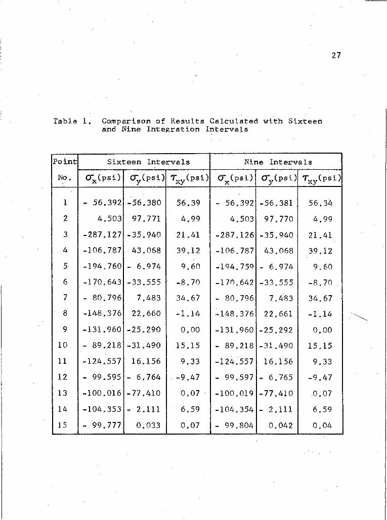
the perforated square plate problem was solved using first sixteen and then nine major integration intervals for a cyclic integration. The fifteen random points were used for the comparison and as Table 1 shows the largest difference is .027% and is in 0"x at node point number 37S. The next largest difference is less than .003%.This comparison indicates, as expected, that the error iri the numerical integration is insignificant „

Truncation of the Series In order for the approximate stress function

to converge to the true stress function the series repre­sentation must be a complete set of coordinate functions„The stress function used in this analysis was presented by J.H. Michell and according to Timoshenko and Goodier (1951, p. 116-117) Michell's Stress Function is complete. Sokolnikoff (1956, p. 262-268) presents Michell's Formu­lation in complex variable form, and completeness of the stress function is implied by Sokolnikoff1s presentation.

The method used here is classified in variational calculus as a direct method. A direct method is a variational method which reduces to a system of ordinary equations as opposed to a system of differential equations.

27

Table 1. Comparison of Results Calculated with Sixteen and Nine Integration Intervals

Point Sixteen Intervals Nine IntervalsNo. O^(psi) CTy(psi) Txy(psi) CTx(psi) <ry(psi) Txy(psi)

1 - 56.392 -56.380 56.39 - 56.392 -56.381 56.342 4.503 97.771 4.99 4.503 97.770 4.993 -287.127 -35.940 21.41 -287.126 -35.940 21.414 -106.787 43.068 39.12 -106.787 43.068 39.125 -194.760 - 6.974 9.60 -194.759 - 6.974 9.606 -170.643 -33.555 -8.70 -170.642 -33.555 -8.70 .7 - 80,796 7.483 34.67 - 80.796 7.483 34.678 -148.376 22.660 -1.14 -148.376 22.661 -1.149 -131.960 -25.290 0.00 -131.960 -25.292 0.00

10 - 89.218 -31.490 15.15 - 89.218 -31.490 15.1511 -124.557 16.156 9.33 -124.557 16.156 9.3312 - 99.595 - 6.764 -9.47 - 99.597 - 6.765 — 9»4713 -100.016 -77.410 0.07 -100.019 -77.410 0.0714 -104.353 - 2.111 6.59 -104.354 - 2.111 6.5915 - 99.777 0.033 0.07 - 99.804 0.042 0.04

Elsgolc (1962, p, 148) discusses the accuracy of the direct methods, and he makes the following statement

' concerning the accuracy of the direct method for a set of coordinate functions, yn :

"Therefore, to determine the exactness of the results, obtained by Ritz1s method or other direct methods, we usually use the following practical method, which does not however have an adequate theoretical foundation. Having computed yn(x) and yn4.j (x), we compare them at some points of the interval (x0 ,x^). If with the degree of exactness required for a given purpose their values coincide, then we consider the solution of the variational problem equal to yn(x)."

According to the quotation, the stress function, Y^-j.,has as many significant figures as the figures repeatedfrom Yjq at .discrete points in the region. It is assumed,therefore, that the same comparison technique may be usedto evaluate the accuracy of the stresses.

This theory is applied to solutions of the per­forated square plate at the fifteen random points.Results obtained using 40 and 41 coordinate functions are tabulated in Table 2. The degree of exactness of the stresses found by a 40 function solution is determined by comparing the stress values obtained using 40 and 41 functions. As may be seen, the stress values are exact to at least the first decimal place.

Computer TruncationThe third source of error, computer truncation,

can only be reduced by a very rigorous selection of

29

Table 2. Results Obtained Using 40 and 41 Coordinate Functions

Po int 40 Functions 41 FunctionsNo. <rx(psi) <Ty (psi) Txy(psi) O^Cpsi) CTXpsi) T y(p sO

1 - 56.395 -56.386 56.40 - 56.395 -56.386 56.402 4.504 97.770 4.98 4.504 97.770 4.983 -287.127 -35.938 21.41 -287.127 -35.398 „21.414 -106.787 43.068 39.12 -106.787 43.068 39.125 -194.760 - 6.973 9.59 -194.760 - 6,973 9.596 -170.642 -33.555 -8.69 -170.642 -33.555 -8.697 - 80.794 7.482 34.67 - 80.794 7,482 34.678 -148,377 22.660 -1.14 -148.377 22.660 -1.149 -131.959 -25.292 0.00 -131.959 -25.293 0.00

10 - 89.219 -31.490 15.16 - 89.219 -31.490 15.1611 -124.558 16.155 9.33 -124.558 16.155 9.3312 - 99.594 - 6.765 -9.46 - 99.594 - 6.765 -9.4613 -100.019 -77.399 0.04 -100.011 -77.398 0.0414 -104.360 — 2,108 6.59 -104.358 - 2.109 6.5915 - 99.740 0.034 0.06 - 99.720 0. 034 0 .06

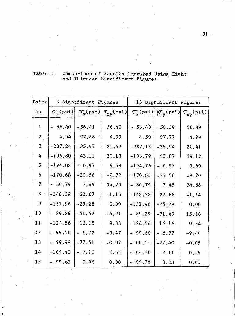
30calculation procedures, and an investigation to determinethe best procedures would be extremely laborious.However, this does not appear to be necessary as a verysimple check has been performed which indicates that thetruncation error is not significant. The check has beenmade by utilizing results at the fifteen random points ofthe perforated square plate (Fig. 4). First the problemwas solved using the IBM 7072 digital computer whichcarries eight significant figures and these results werethen compared to results obtained with the GDC 6400

" - digital computer which carries thirteen significantfigures. This comparison is displayed in Table 3, andit may be seen that the maximum difference for stressesgreater than 2 psi is less than 1%. For stresses ofmagnitude, greater than 5 psi the difference is muchless than 1%.

31

Table 3. Comparison of Results Computed Using Eight and Thirteen Significant Figures

Point 8 Significant Figures 13 Significant FiguresNo. CTx(psi) (TyCpSi) Txy(psl) crx(psi) jq^(psi) Txy(Psi)

1 -.56.40 -56.41 56,40 — 56,40 -56.39 56.392 4.54 97,88 4.99 4.50. 97.77 4.993 -287.24 -35,97 21.42 -287.13 -35.94 21.414 -106.80 43.11 39.13 -106.79 43.07 39.125 -194.82 - 6.97 9.58 -194.76 - 6.97 9.606 -170.68 -33.56 -8.72 -170.64 -33.56 -8.707 - 80.79 7.49 34.70 — 80.79 7.48 34.688 -148.39 22.67 -1.16 -148.38 22.66 -1.149 -131,96 -25.28 0.00 -131.96 -25.29 0.00

10 - 89.28 -31.52 15.21 - 89.29 -31.49 15.1611 -124.56 16.15 9.33 -124.56 16.16 9.3412 — 99,56 - 6.72 -9.47 - 99.60 - 6.77 -9.4613 - 99.98 -77.51 —0.07 -100.01 —77.40 -0.0514 —104.40 - 2.10 6.63 -104.36 - 2.11 6.5915 - 99.43 0.06 0.00 - 99.72 0.03 0.01

CHAPTER 4

VERIFICATION OF THE METHOD

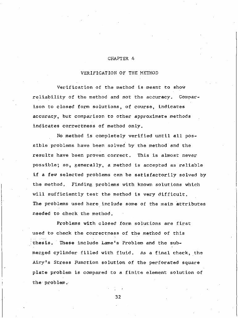
Verification of the method is meant to show reliability of the method and not the accuracy. Compar­ison to closed form solutions, of course, indicates accuracy, but comparison to other approximate methods indicates correctness of method only.

No method is completely verified unti1 all pos­sible problems have been solved by the method and the results have been proven correct. This is almost never possible; so, generally, a method is accepted as reliable if a few selected problems can be satisfactorily solved by the method, Finding problems with known solutions which will sufficiently test the method is very difficult.The problems used here include some of the main attributes needed to check the method.

Problems with closed form solutions are first used to check the correctness of the method of this thesis. These include Lame1s Problem and the sub­merged cylinder filled with fluid. As a final check, the Airy's Stress Function solution of the perforated square plate problem is compared to a finite element solution of the problem.

32

33Closed Form Solutions

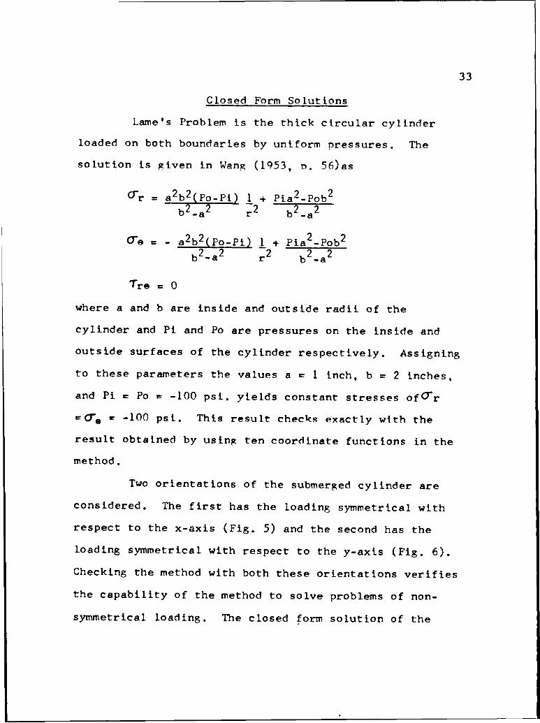
Lame's Problem is the thick circular cylinder loaded on both boundaries by uniform pressures. The solution is given in Wang (1953, n . 56)as

^ r = a^b^CPo-Pi) 1 *f Pia^-Pob^" T O ? “ O '

= - a^b^(Po-Pi) 1_ ^ Pia^-Pob^ b2-a2 r2 b^-aZ

Tre = 0where a and b are inside and outside radii of the cylinder and Pi and Po are pressures on the inside and outside surfaces of the cylinder respectively. Assigning to these parameters the values a = 1 inch, b = 2 inches, and Pi c Po = -100 psi. yields constant stresses of0"r c 0"e = -100 psi. This result checks exactly with the result obtained by using ten coordinate functions in the method.

Two orientations of the submerged cylinder are considered. The first has the loading symmetrical with respect to the x-axis (Fig. 5) and the second has the loading symmetrical with respect to the y-axis (Fig. 6).Checking the method with both these orientations verifiesthe capability of the method to solve problems of non- symmetrical loading. The closed form solution of the

34

Outside Diameter = 2 inches Inside Diameter = 1 inch P0 = -50(l-cos6) psi

= -100(1-cos©) psi

Fig. 5. Submerged Cylinder Filled with Fluid so that the Loading is Symmetrical with

Respect to the X-axis

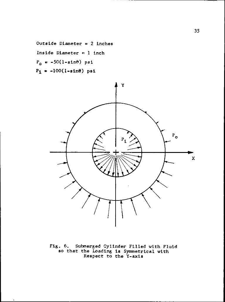
35

Outside Diameter = 2 inches Inside Diameter = 1 inch P0 *= -50(l-sin6) psi Pj. « -100(l-sin8) psi

Fig. 6. Submerged Cylinder Filled with Fluid so that the Loading is Symmetrical with

Respect to the Y-axis

36submerged cylinder problem is obtained by choosing (for the first case) the stress function

Y = G 2 6 rsin6 - [(l-v)/2]rlnrcosA + C0

+ C^r^ 4- Cglnr + (C^r + C^r^ + C^r^^cosB

where Y satisfies the biharmonic equation. Then the boundary conditions are satisfied exactly by equating the radial stresses on the boundaries as found with the stress function to the boundary tractions. The constant G 2 is found from the resultant of the tractions on the outer boundary. A solution to the first case yields the following coordinate function coefficients:

G2 = 50

Cj = - 1 0 0 / 6 = - 1 6 .6 6 6 7

C2 = 200 /3 = -6 6 .6 6 6 7

C3 = 107 .37

C4 = 1 .875

C5 = - 7 . 5 0

The same coefficients as found by the method using twenty-four coordinate functions are

= - 1 6 . 6 6 7

C2 = -66.666 C3 = 107 .37

C4 = 1 .8749

37

C5 = “7,5003

while the remaining nineteen coefficients are

Cfi ~ Gy ™ ° — C24 — 0

A similar result was obtained for the second case, that is, with the loading symmetrical to the y-axis.

Finite Element Comparison A finite element program is used to solve for the

stresses in the uniaxialy stressed perforated square plate. The program was developed by Dr. Richard, Professor of Civil Engineering, The University of Arizona, Tucson, Arizona, and Hr. Callabresi, N.S.F. Graduate Fellow, Department of Civil Engineering, The University of Arizona, Tucson, Arizona.

Thfe finite element model is the constant stress, triangular plate element. Stresses at discrete points in the region are found by averaging the stresses of adjacent triangular elements (Turner, Martin, and Weike1 1964),The accuracy of the results depends on the number of elements used in the solution and on the distribution of the elements. Good stress results may be expected if a sufficient number of elements are used and the elements are distributed in such a manner that a large number of elements are clustered in the regions of drastically varying stresses.

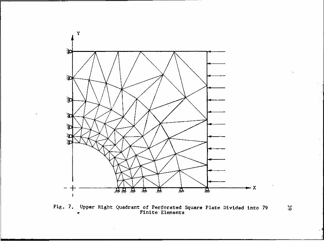
38Shown in Fig. 7 is the distribution of triangular

elements which is used in the analysis of the perforated plate. Lateral displacements on the x and y axes are constrained because the boundaries along these axes are known to remain, straight. The elements are chosen smaller near the circular boundary because the gradients of the stresses increase in the vicinity of the circular boundary.

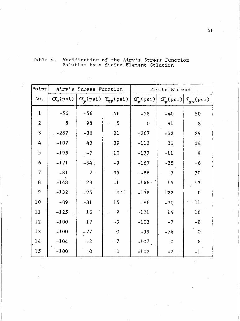
Again the stresses at the fifteen random points (Fig, 4) are used for comparison. The results of the method using 40 coordinate functions are rounded off and are compared to the finite element results in Table 4.Stress values for the boundary points 1, 13, and 15 are found by using an extrapolation technique.

When one of the three stresses (Ox, Oy, or Txy)at a point is much higher than either of the other two,the finite element analysis does not predict good valuesfor the smaller stresses. Even though this causesrelatively large percentage discrepancies in the smallerstress values, the absolute values of the differencesare not entirely unreasonable. Considering the accuracylimitations of the finite element approach, the agreementof stress values in Table 4 seems quite good for verificationof the method. The largest absolute difference of stressesis found in CT at point number three, and this difference x ’

Y

I

7. Upper Right Quadrant of Perforated Square Plate Divided into 79 • Finite Elements

is only 20 psi which is less than 10% of the stress value. As a further check on the method, the stresses

were calculated at fourteen points on the boundaries.The maximum error in the calculated stresses was at a corner point.and was .3 psi. For the remaining thirteen points, the calculated stresses were in error by less than .03 psi.

41

Table 4. Verification of the Airy8s Stress Function Solution by a finite Element Solution

Point Airy1s Stress Function Finite ElementNo. O^(psi) c y p s D T x y ( p s i ) < y psi) CT,(psi) Txy(psi)

1 -56 —56 56 -58 -40 502 5 98 5 0 91 83 "287 -36 21 -267 -32 294 "107 43 39 -112 33 345 -195 -7 10 -177 "11 96 -171 "34 : -9 -167 -25 — 67 -81 7 35 —86 7 308 -148 23 -1 -146 ■ 15 139 -132 -25 - 0 . ' -136 122 010 "89 -31 15 -86 -30 1111 -125 , . 16 ■ 9 -121 14 1012 — 100 17 -9 — 103 -7 -813 "100 -77 0 -99 -74 014 -104 -2 ■ 7 -107 0 615 -100 0 0 -102 -2 - 1

\

CHAPTER 5

CONCLUSIONS AND FUTURE INVESTIGATIONS

For the problems considered, the method of Airy's Stress Function with the Modified Trefftz1s Procedure has been shown to give excellent results.Any other plane elasticity problem defined by a doubly connected region with known boundary tractions can also be solved by the method, If an extremely large number of coordinate functions is used in the solution or if the mathematical representation of the boundary tractions is very complex, the accuracy of the numerical integration should be improved by increasing the number of quadrature points in the Gauss's Quadrature Formulae,

Erroneous results were obtained during the investigation of the method when only one major interval of integration was used for a cyclic integral along an inside boundary. This undesirable effect is thought to be caused by overly wide spacing of the quadrature points. If the quadrature points are too widely spaced, the oscillations of the integrand along the interval of integration may not be properly registered in the numerical integration. The maximum allowable spacing for reliable numerical integration could possibly be determined by

42

43future investigations.

Another worthwhile investigation would be the evaluation of different coordinate functions as solution mechanisms. Although Michell's Formulation provides a good set of functions, some other formulations might yield more rapidly convergent series.

Since the method does give good results for doubly connected regions, the same concepts could probably be extended to multiply connected regions. Such an extension would require the inclusion of additional branch cuts and the evaluation of the gradient of the stress function at the branch cut of each additional boundary curve.Also, another set of coordinate functions similar to that of Michell's Formulation would need to be added to the approximate stress function for each additional boundary curve"(Timoshenko and Goodier 1951, p. 120).

REFERENCES

Allen$ D.N. de G., Relaxation Methods In Engineering and Science. Me Gnaw-Hill Book Company, Inc.,New York, 1954.

Elsgolc, L.E., Calculus of Variations. Addison-Wesley Publishing Company Inc., Massachusetts$ 1962.

Fox, Charles, An Introduction to the Calculus of Varia­tions . Oxford University Press. London- 1954.

Scarborough, James B., Numerical Mathematical Analysis.4th Edition, The John Hopkins Press, Baltimore, 1958.

SokoInikoff, I.S., Mathematical Theory of Elasticity.2nd Edition, McGraw-Hill Book Company, Inc.,New York, 1956.

Timoshenko, S. and J.N. Goodier, Theory of Elasticity.McGraw-Hill Book Company, Inc., New York, 1951.

Turner, M .J., Martin, B.C., and Weikel, "Further Develope- ments and Applications of the Stiffness Method", Matrix Methods of Structural Analysis (edited by F. de Veubeke), AGARDograph 72, The MacMillan Company, 1964. .

44