AIRS Project

Algorithm Theoretical Basis Document

Level l b

Part 3: Microwave Instruments

Bjorn H. Lambrigtsen

Jet Propulsion Laboratory California Institute of Technology

D-17005 Version 2.0

15 December 1999

Version history

Version 1.0 September 1996 Initial draft version

Version 12 November 1996 First released version Minor editing changes

Version 2.0 December 1999 Second released version Changed MHS references to HSB Added measured AMSU-A NEDT values Added section on instrument synchronization and alignment Added details on blackbody PRT placement Revised processing parameters related to sun glint Added discussion of redundant PRT’s and PLLO’s Revised discussion of lunar contamination Revised description of space view sidelobe correction Reorganized sections on antenna and brightness temperatures Revised description of sun glint algorithm Added description of algorithm to estimate radiometric accuracy Added preliminary description of coast contamination algorithm Added discussion of quality assessment Added section on post-launch validation and verification

Table of Contents

I

Introduction

1 Historical Perspective 1.1 Temperature sounder - AMSU-A 1.2 Humidity sounder - HSB

2 Instrument Description 2.1 AMSU-A 2.2 HSB 2.3 Instrument interoperability

3 In-flight Calibration System 3.1 Blackbody view 3.2 Cold space view 3.3 Sources of errors and uncertainties

4 Relevant Data 4.1 Pre-launch testing and characterization 4.2 Processing parameters and tables 4.3 Telemetry

5 Computation of Radiometric Calibration Coefficients 5.1 Effective blackbody brightness 5.2 Effective space brightness 5.3 Radiometric calibration counts 5.4 Smoothed calibration counts 5.5 Calibration coefficients

6 Computation of Brightness Temperatures 6.1 Radiometric calibration 6.2 Far sidelobe correction 6.3 Near sidelobe correction 6.4 Estimated radiometric accuracy 6.5 Estimated calibration accuracy 6.6 Sun glint 6.7 Coast contamination 6.8 Quality assessment

7 Post-Launch Verification and Validation 7.1 Radiometric validation- 7.2 Spatial calibration

Appendix A Quality assessment parameters (draft)

1

2 4 5

6 7

13 16

17 20 21 22

25 25 25 26

27 28 32 35 37 39

41 41 41 43 43 43 44 45 45

47 47 47

49 49

i

Illustrations

Figure 1 Figure 2 Figure 3 Figure 4 Figure 5 Figure 6 Figure 7 Figure 8 Figure 9 Figure 10 Figure 11 Figure 12 Figure 13 Figure 14 Figure 15

AMSU-A 1 physical configuration AMSU-A2 physical configuration AMSU-A antenna and RF feed system (schematically) Typical AMSU-A antenna pattern AMSU-A 1 RF front end AMSU-A2 RF front end Scan sequence AMSU-A polarization vectors HSB/AMSU-B physical configuration AMSU-B antenna and RF feed system AMSU-B RF receiver Radiometer transfer function AMSU-A1 calibration target Unobstructed cold-space view sector Smoothing function

Tables

7 8 8 9

10 10 11 12 13 14 14 18 20 21 37

Table 1 AMSU-A channels characteristics 11 Table 2 HSB channel characteristics 15 Table 3 Processing parameters and tables 25 Table 4 AMSU-A1 engineering data used for calibration processing 26 Table 5 AMSU-A2 engineering data used for calibration processing 26 Table 6 HSB engineering data used for calibration processing 26

11 ..

Acronyms and abbreviations

A/D AIRS AMSU ARM ATBD CART DAAC DMSP DN DOD DOE EOS EOSDIS EU FRD GSFC HIRS HSB ICD IF IR ITS JPL LO MHS MIT MSU MUX MW NASA NEDT NOAA NWS PGS PLLO PRT QA RF SCAMS SIRS SSM/IS SSMiT TIROS TLSCF TOVS VIS WMO

Analog-to-digital Atmospheric Infrared Sounder Advanced Microwave Sounding Unit Atmospheric Radiation Measurement program Algorithm Theoretical Basis Document Cloud and Radiation Testbed Data Active Archive Center Defense Meteorological Satellite Program Data number Department of Defense Department of Energy Earth Observing System EOS Data and Information System Engineering unit Functional Requirements Document Goddard Space Flight Center High Resolution Infrared Radiation Sounder Humidity Sounder for Brazil Interface Control Document Intermediate frequency Infrared Interagency Temperature Sounder Jet Propulsion Laboratory Local oscillator Microwave Humidity Sounder Massachusetts Institute of Technology Microwave Sounding Unit Multiplexer Microwave National Aeronautic and Space Administration Noise-equivalent delta-T National Oceanic and Atmospheric Administration National Weather Service Product Generation Subsystem Phase locked local oscillator Platinum resistance thermometer Quality assessment Radio frequency Scanning Microwave Spectrometer Satellite Infrared Radiation Spectrometer Special Sensor - Microwave Imager/Sounder Special Sensor - Microwave Temperature sounder Television Infrared Observation Satellite Team Leader Science Computing Facility TIROS Operational Vertical Sounder Visible World Meteorological Organization

... 111

EOS-PM1 Spacecraft - “Aqua”

iv

Introduction

This is Part 3 of the AIRS Level l b Algorithm Theoretical Basis Document (ATBD). While Part 1 covers the infrared spectrometer and Part 2 the associated visiblelnear infrared channels (i.e. the Atmospheric Infrared Sounder - AIRS proper), Part 3 covers the microwave instruments associated with AIRS - the Advanced Microwave Sounding Unit A (AMSU-A) and the Humidity Sounder for Brazil (HSB).

The Level l b ATBD describes the theoretical basis and, to some extent, the form of the algorithms used to convert raw data numbers (DN) or engineering units (EU) from the telemetry of the various instruments to calibrated radiances. The former (i.e. raw and minimally processed telemetry) are Level l a products and make up the input to the Level 1 b process, while the latter - the output from the Level 1 b process - make up the input to the Level 2 process, where the radiances are converted to geophysical parameters.

The algorithms described in this document follow closely those which have been developed by NOAA1.2 for a near-identical set of instruments, flown for the first time in 1998. Although more sophisticated algorithms may be available, our intention is to initially deviate only minimally @om the NOAA approach. We expect to revise the algorithms based on operational experience with the instruments. The only major difference is that while NOAA prefers to convert radiometer measurements to physical radiance units (mW/m2-sr-cm-l) we will convert to brightness temperatures instead, which is the most common practice in the microwave field. It is a simple matter to convert between the two (see, e.g., m. (5-17) in Section 5 ) .

It is the intention that each part be readable as a standalone document, although it is recommended that the reader reference related instrument and system description documents, such as the Aerojet document referred to on p . 15. In what follows there is a brief description of each of the microwave instruments, in order to explain references to devices, procedures and tables used by the Level l b algorithms. However, for a full understanding of the hardware and the measurement system, the reader should also refer to the AIRS Level l b ATBD Part 1 , the AIRS, AMSU-A4 and HSB/AMSU-B5 Functional Requirements Documents (FRD’s), and relevant hardware description documents. The present document reflects as-built performance characteristics to the extent they are known, and otherwise assumes full compliance of the hardware with the respective FRD’s.

This document describes the functions performed by the data processing system. However, it should be noted that nothing is implied about the architecture or the implementation of the system. Thus, algorithms which may be described here as if they were to be executed adjacently could in fact be executed non-adjacently. For example, some data quality checking is described in each section. Such modules may be consolidated and executed before that section is reached in the actual processing system, in order to provide an efficient implementation.

D. Q. Wark, Private communication (1996) R. Amick, AMSU Calibration Processing, http://psbsgi 1 .nesdis.noaa.gov:8080/KLM/Pages/AMSUpro.html M. T. Chahine, “AIRS Functional Requirements Document”, NASNJPL #D-8236 (1992) NASA/GSFC, “Performance and Operation Specifications for EOS AMSU-A”, #9480-80 (1994) D. R. Pick, “Specification for AMSU-B“, U.K. Met. OfSice #O 19/11/20/4 (1987)

1

1 Historical Perspective

The Advanced Microwave Sounding Unit A (AMSU-A) and the Humidity Sounder for Brazil (HSB), together with the Atmospheric Infrared Sounder (AIRS) - a high spectral resolution IR spectrometer - are designed to meet the operational weather prediction requirements of the National Oceanic and Atmospheric Administration (NOAA) and the global change research objectives of the National Aeronautics and Space Administration (NASA). The three instruments will be launched in December 2000 on the NASA EOS- PM1 spacecraft (recently named the “Aqua”).

The HIRS (High Resolution Infrared Sounder) and the Microwave Sounding Unit (MSU) on the NOAA polar orbiting satellite system have supported the National Weather Service (NWS) weather forecasting effort with global temperature and moisture soundings since the late 70’s. After analyzing the impact of the first ten years of HIRS/MSU data on weather forecast accuracy, the World Meteorological Organization in 19876 determined that global temperature and moisture soundings with radiosonde accuracy are required to significantly improve the weather forecast. Radiosonde accuracy is equivalent to profiles with 1K rms accuracy in 1-km thick layers and humidity profiles with 20% accuracy in 2-km thick layers in the troposphere.

The Interagency Temperature Sounder (ITS) Team, with representatives from NASA, NOAA and DOD, was formed in 1987 to convert the NOAA requirement for radiosonde accuracy retrievals to measurement requirements of an operational sounder. An extensive effort of data simulation and retrieval algorithm development was required to establish instrument measurement requirements for spectral coverage, resolution, calibration, and stability; spatial response characteristics including alignment, uniformity, and measurement simultaneity; and radiometric and photometric calibration and sensitivity.

This NOAA requirement went far beyond the capability of the HIRS sensor technology. However, breakthroughs in IR detector array and cryogenic cooler technology by 1987 made this requirement realizable with technology available for launch at the end of this century. AIRS is the product of this new technology. AIRS, working together with AMSU-A and HSB, forms a complementary sounding system for NASA’s Earth Observing System (EOS) and the NOAA-derived requirements are reflected in the respective Functional Requirements Documents.

The measurement concept employed by AIRS/AMSU-A/HSB follows the concept originally proposed by Kaplan7 in 1959, verified experimentally ten years later using measurements from the Satellite Infrared Radiation Spectrometer (SIRS), and the relaxation inversion algorithm published by Chahine8. This approach is still used operationally by the HIRSIMSU system. Temperature and moisture profiles are measured by observing the upwelling radiance in the carbon dioxide bands at 4.2 ym and 15 ym and the water band at 6.3 pm for HIRS/AIRS, and in the 50-60 GHz oxygen band for MSU/AMSU-A9 and the 183-GHz water line for HSB (no MSU equivalent). However, compared to the HIRS spectral resolution of about 50, AIRS will have a spectral resolution of 1200. The high spectral resolution gives sharp weighting functions and

“The World Weather Watch Programme 1988-1997“, WMO-No. 691 (1987) L. D. Kaplan, Inference of atmospheric structures from satellite remote radiation measurements, J . Opt.

M. T. Chahine, Determination of the temperature profile in an atmosphere from its outgoing radiance, J .

The microwave temperature sounding concept employed by MSU was first tested with SCAMS.

Soc. Am., 49, 1004-1007 (1959)

Opt. Soc. Am., 58,1634-1637 (1968)

See D. H. Staelin et al., The Scanning Microwave Spectrometer (SCAMS) Experiment: The Nimbus 6 User’s Guide, NASA/GSFC (1975)

2

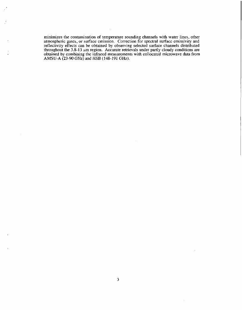
minimizes the contamination of temperature sounding channels with water lines, other atmospheric gases, or surface emission. Correction for spectral surface emissivity and reflectivity effects can be obtained by observing selected surface channels distributed throughout the 3.8-13 pm region. Accurate retrievals under partly cloudy conditions are obtained by combining the infrared measurements with collocated microwave data from AMSU-A (23-90 GHz) and HSB (14.8-191 GHz).

3

1.1 Temperature sounder - AMSU-A

AMSU-A is primarily a temperature sounder. Its most important function is to provide atmospheric information in the presence of clouds which can be used to correct the infrared measurements for the effects of the clouds. This is possible because microwave radiation passes, to a varying degree, through clouds - in contrast with visible and infrared radiation, which is stopped by all but the most tenuous clouds. This cloud clearing technique has been demonstrated to work well for scenes which are partially cloudy - at up to 75-80% cloud cover, and is used routinely by NOAA as part of the operational processing of TOVS data.

The instrument is a direct descendant of the MSU. While MSU was designed and built by the NASA Jet Propulsion Laboratory (JPL), AMSU-A is being built by Aerojet - a commercial aerospace company - under the auspices of NASA. Although NASA's AMSU-A is not due to be launched until 2000, a series of three nearly identical instruments have already been built for NOAA, as a follow-on to the MSU series - the last one of which has now been launched and is operating on the NOAA-14 platform. The first AMSU-A was launched, as part of the NOAA Advanced TOVS system, on NOAA- K (now NOAA-15) in May 1998. It has performed very well.

Although the basic measurement and instrument concepts are the same, the capabilities of AMSU-A significantly exceed those of MSU. Thus, while MSU has only four channels (in the 50-GHz oxygen band for temperature sounding) and samples eleven 7.5" scenes per 26.5-second crosstrack scan, AMSU-A has twelve temperature sounding channels as well as three moisture and cloud channels and samples thirty 3.3" scenes per 8-second crosstrack scan. The size of an AMSU-A "footprint" at nadir is therefore less than half the size of an MSU footprint. The larger number of sounding channels also allows denser spectral resolution of the oxygen band, which results in a greater vertical resolution. The measurement density of AMSU-A is more than 30 times that of MSU. (For reference, it may be noted that the measurement density of AIRSIR is about 1500 times that of AMSU-A and that of AIRS/VIS about 130 times that of AMSU-A.)

It should also be mentioned that the Department of Defense has been operating an instrument somewhat similar to MSU on its Defense Meteorological Satellite Program (DMSP) series of satellites since 1979 - the SSM/T. Built by Aerojet, the SSM/T has seven temperature sounding channels and samples seven 12" scenes per 32-second crosstrack scan, with a measurement density about the same as for MSU.

4

1.2 Humidity Sounder - HSB

HSB is primarily a humidity sounder. Its function is to provide supplementary water vapor and liquid data to be used in the cloud clearing process described above.

This instrument is a direct descendant of what was originally intended to form a part of the AMSU system. AMSU-A was to be the temperature sounder and AMSU-B was to be the moisture sounder. This concept survived, albeit as separate instruments with different spatial resolutions. AMSU-B has now been built, by the former British Aerospace under the auspices of the United Kingdom Meteorology Office, and was launched along with AMSU-A on the newest generation of NOAA platforms, NOAA-K (now NOAA-15), in May 1998. This system now has operational status. The performance of AMSU-B has been disappointing, due to its unanticipated susceptibility to interference from the spacecraft transmitters. However, the RF shielding of HSB has been modified and enhanced, and HSB is not expected to exhibit this susceptibility. (The same is true for the remaining two AMSU-B flight models, to be launched in the next few years.)

HSB is a a near identical copy of AMSU-B, and is now being built by the same branch of Matra Marconi Space which built AMSU-B (formerly a branch of British Aerospace), under contract with Brazil's National Institute for Space Research (INPE). The original plan was for EUMETSAT to supply a new version of this this instrument, the Microwave Humidity Sounder (MHS), to NASA for support of AIRS on the EOS-PM1 platform. However, no agreement was reached between NASA and EUMETSAT, and as a consequence MHS will not be part of the AIRS instrument suite.

The microwave moisture sounding capabilities are viewed as very important to the success of the EOS mission, and efforts were made to find a replacement for the "missing1' HSB. Fortunately, the Brazilian Space Agency (AEB) offered to procure a copy of AMSU-B, the HSB, and provide it for use on EOS-PM1. Due to budget constraints, HSB implements only four of the five AMSU-B channels, but is otherwise functionally identical to AMSU-B. (Some minor modifications have been made to account for for the EOS orbit being different from the TIROS orbit, and some parts are different and from new suppliers.) Since one of the AMSU-B channels is at the same frequency as one of the AMSU-A channels (89 GHz), the AIRS Science Team has judged the loss of this channel to be acceptable.

HSB has four moisture sounding channels. One so-called window channels (at 150 GHz) measures a part of the water vapor spectral continuum, while three are grouped around the 183-GHz water vapor absorption line. Like AMSU-B it samples ninety 1 .lo scenes per 2.67-second crosstrack scan. Due to the higher spatial resolution (which equals that of AIRS) and a higher scan rate, the measurement density is 2.4 times that of AMSU-A (20% less than for AMSU-B).

It should also be mentioned that the Department of Defense has been operating an instrument somewhat similar to AMSU-B as part of the DMSP series since 1991 - the SSM/T-2. Built by Aerojet, this instrument has five channels virtually identical to the AMSU-B channels and samples twentyeight 3.3-6" scenes per 8-second crosstrack scan. The measurement density is therefore about 10 times less than that of AMSU-B. A nearly identical version of this instrument will also form part of the next-generation DMSP conical scanner (SSM/IS), soon to be launched for the first time.

5

2 Instrument Description

In this section we give a brief description of the two microwave instruments, AMSU-A and HSB. (The former is really two instruments, as will become apparent.) Much of the information used to describe HSB pertains equally well to AMSU-B, since the two are virtually identical. Footnotes and comments will point out the differences, where appropriate.

6

2.1 AMSU-A

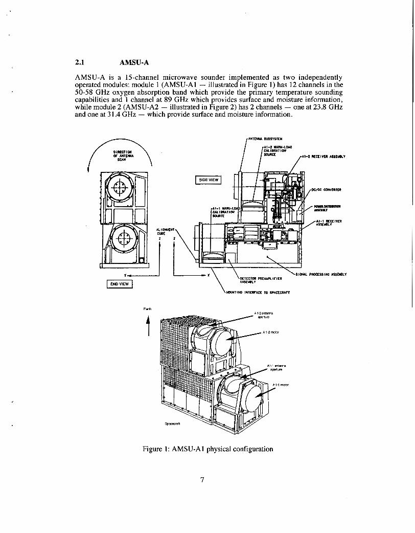
AMSU-A is a 15-channel microwave sounder implemented as two independently operated modules: module 1 (AMSU-A1 - illustrated in Figure 1) has 12 channels in the 50-58 GHz oxygen absorption band which provide the primary temperature sounding capabilities and 1 channel at 89 GHz which provides surface and moisture information, while module 2 (AMSU-A2 - illustrated in Figure 2) has 2 channels - one at 23.8 GHz and one at 3 1.4 GHz - which provide surface and moisture information.

\

r .

I ENDVIEW I

E am A 1-2 andem

t

Figure 1: AMSU-A1 physical configuration

7

Figure 2: AMSU-A2 physical configuration

Like AIRS, AMSU-A is a crosstrack scanner. The three receiving antennas - two for AMSU-A1 and one for AMSU-A2 - are parabolic focusing reflectors which are mounted on a scan axis at a 45" tilt angle, so that radiation is reflected from a direction perpendicular to the scan axis into a direction along the scan axis (i.e. a 90" reflection). Thus, radiation from a direction within the scan plane, which depends on the angle of rotation of the reflector, is reflected and focused onto the receiver aperture - a conical feedhorn. This is illustrated in Figure 3.

Figure 3: AMSU-A antenna and RF feed system (schematically)

8

The design of the antenna system is such that a slightly diverging conical "beam" is formed which has a half-power width (also called the 3-dB width) of approximately 3.3", with a *lo% variation from channel to channel. The diameters of the reflectors are 13.2 cm (5.2") for AMSU-A1 and 27.4 cm (10.8") for AMSU-A2. The beam is approximately Gaussian-shaped at the center and receives a significant portion of its energy outside the half-power cone. Approximately 9597% of the energy is received within the so-called main beam, which is defined as 2.5 times the half-power beam - i.e. the AMSU-A main beam is 8.25" wide. Significant energy (i.e. up to 5%) is thus received from outside the main beam. Figure 4 shows a typical AMSU-A antenna pattern. The pattern in the vicinity of the main beam is called the near sidelobes, while that further away is called the far sidelobes. The far sidelobes contribute significantly to the uncertainty of the measurements.

-i80 -120 -80 0 . 0 *eo 120 SCAN ANOCE (LEO)

Figure 4 Typical AMSU-A antenna pattern

The feedhorn is followed by a multiplexer which splits the RF energy into two or more parallel signal paths which proceed to the receiver - a heterodyne system, where each channel is down converted, filtered and detected. AMSU-A1 has two such RF front ends (Figure 5), while AMSU-A2 has one (Figure 6) .

It should be emphasized that AMSU-A1 and AMSU-A2 are two completely independent instrument modules, with separate power, telemetry and command systems. They are even mounted independently on the spacecraft. The two AMSU-AI receivers, on the other hand, are tightly coupled and share main system resources. The most notable exception to that is that the two antennas are scanned independently - although they share a common scan control system. Therefore, the scan positions of both antennas are reported in the telemetry.

The antenna reflectors rotate continuously counter-clockwise relative to the spacecraft direction of motion (i.e. the x-axis), completing one revolution in 8 seconds. (The three scan mechanisms are all synchronized to the spacecraft clock, to within a few milliseconds.) Such an 8-second scan cycle is divided into three segments. In the first segment the earth is viewed at 30 different angles, symmetric around the nadir direction, in a step-and-stare sequence. The antenna is then quickly moved to a direction which points it toward an unobstructed view of space (i.e. between the earth's limb and the

9

AMSU-A1 antenna subsystem AMSU-A1 receiver subsystem

Figure 5: AMSU-A1 RF front end

i WC.mnlC I I I

I eac%@wld CSlbaRlm

I I

SMKa I

AMSU-A2 antenna subsystem AMSU-A2 receiver subsystem

Figure 6: AMSU-A2 RF front end

spacecraft horizon) and stopped while two consecutive cold calibration measurements are taken. Next, the antenna is again quickly moved to the zenith direction, which points it toward an internal calibration target which is at the ambient instrument temperature, and stopped while two consecutive warm calibration measurements are taken. Finally, the

10

antenna is again quickly moved to the starting position to await the synchronization signal to start a new scan cycle. Figure 7 illustrates this - the normal operational scan mode. (There is also a stare mode, where the antenna is permanently pointed to the nearest-nadir direction, but that is only used for special purposes - such as for spatial calibration using coast line crossings.) Each of the 30 earth views (scene stations) takes about 0.2 seconds, for a total of approximately 6 seconds. The actual integration time is somewhat less - approximately 0.165 seconds per view for AMSU-A1 and 0.158 seconds per view for AMSU-A2. The calibration system will be described in Section 3.

Zenllh

Slew 2

0.400 Sac

Slew 3 131.661’

5.965 Sec Nadir

Figure 7: Scan sequence

Table 1: AMSU-A channel characteristics

lo Aerojet, “AMSU-A Calibration Log Book’, Reports 11320 & 11 192 (1998) l 1 Polarization angles, referenced to the horizontal plane, are 90”-rp for “V” andrp for “H”, where rp is the scan angle

11

The characteristics of each channel are listed in Table 1 . The table lists three frequency specifications: nominal center frequency, center frequency stability (i.e. the maximum deviation expected from the nominal center frequency value) and as-built bandwidth. All are given in MHz. The bandwidth notation is "Nxbf", where is N is the number of sub- bands used for a channel and h f is the width of each sub-band. (E.g., 2x270 means this is a double-band channel, with each of the two bands being 270 MHz wide.) The quantity listed as NEDT - the noise-equivalent AT - is a measure of the thermal noise in the system. It is equivalent to the standard deviation of the signal which would be measured if a 300 K target were observed by the system, i.e. it is the standard deviation of the thermally induced fluctuations. Both measured (as-built) and required NEDT values are listed.

The RF feed selects, for each channel, a linear polarization which is fixed relative to the feedhorn. However, due to the rotating scan reflector the selected polarization is not fixed relative to the scan plane (and therefore relative to the earth). Rather, it rotates as the antenna reflector rotates. Thus the polarization vector for channels labeled "V" forms an angle cp with the scan plane, while the "H"-polarization direction forms an angle 90"- cp with the scan plane. At nadir the two directions are in the scan plane and perpendicular to the scan plane, respectively. This is illustrated in Figure 8, which shows the various polarization vectors in the plane of the electromagnetic field vectors - i.e. in a plane perpendicular to the direction of propagation. (At nadir, this plane coincides with the horizontal plane, while at a scan angle of cp it is tilted from the local horizontal plane by an angle equal to the local angle of incidence.)

""""

I k n t e r s e c t i o n with scan plane I

True V (plane of incidence)

"H" True H

""""

Intersection with local horizontal'ijlane

Figure 8: AMSU-A polarization vectors

12

2.2 HSB

HSB is a 4-channel microwave moisture sounder implemented as a single module. Physically it is identical to AMSU-B, which is illustrated in Figure 9.

Earth

Figure 9: HSB/AMSU-B physical configuration

HSB is very similar to AMSU-A. We will therefore only give a very brief summary of the pertinent characteristics and otherwise refer the reader to the description Of AMSU-A (see 2.1).

There is only one antenna. It has a half-power beamwidth of 1 . l o , i.e. one-third of the AMSU-A beamwidth and nominally equal to that of AIRS. The diameter of the reflector aperture is 21.9 cm (8.6"). The shape of the "beam" is also similar to that of AMSU-A: it is nearly gaussian near the center, it receives 96-98% of its energy within the main beam - which is 2.75" wide (2.5 times the half-power width) and 99% within an 8" cone. HSB/AMSU-B uses a continuously scanning motor (i.e. not a stepper motor). The radiation is sampled "on the fly", approximately every 18 ms. The sample cells, defined by the half-power contours, are therefore motion smeared and overlap each other. The effective, motion smeared, beam width in the scan direction is approximately 1.4".

Unlike AMSU-A, there is more than a single feedhorn, however. Figure 10 shows how the single antenna beam is split into three paths with dichroic plates and directed into three feedhorns. One feedhorn is used for the 89-GHz signal, one is used for the 150-GHz signal, and one is used for the 183-GHz signal. The latter is followed by a triplexer which allows three 183-GHz channels to be separated out. Figure 1 1 shows a diagram of the AMSU-B receiver. Note that for HSB the 89-GHz feedhorn and associated receiver components are absent.

Table 2 lists the specified characteristics of the HSB channels.

13

DICHROIC PLATES Z I

Figure 10: AMSU-B antenna and RF feed system

Figure 11: AMSU-B RF receiver

14

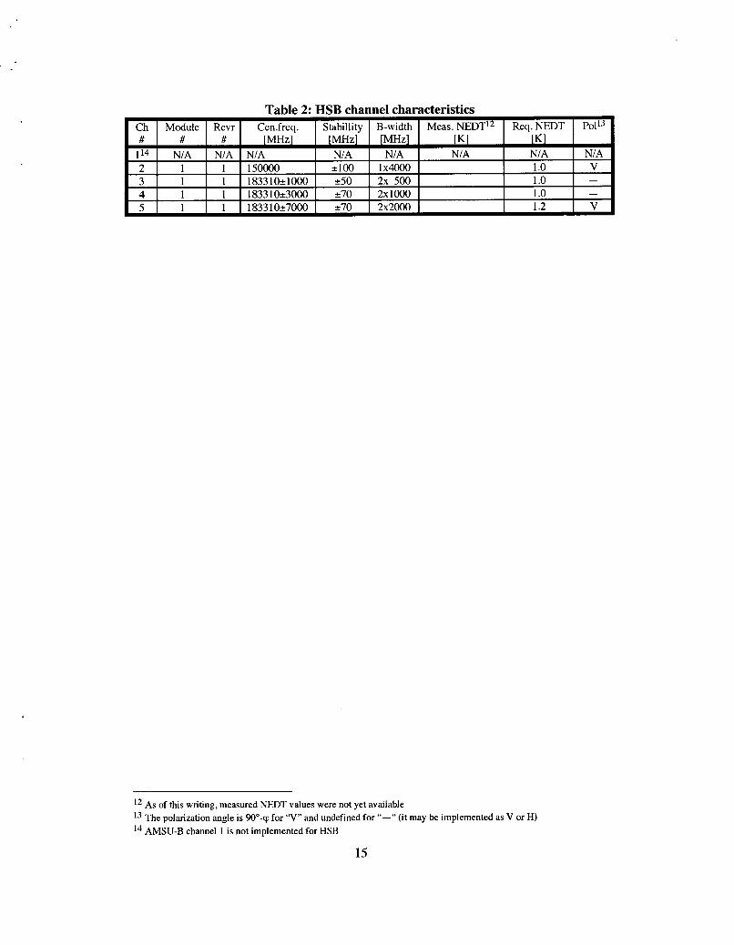
l2 As of this writing, measured NEDT values were not yet available l3 The polarization angle is 9O"-cp for "V" and undefined for "-'' (it may be implemented as V or H) l4 AMSU-B channel 1 is not implemented for HSB

15

2 3 Instrument Interoperability

As described earlier, the AIRS/AMSU-A/HSB instrument suite forms a single sounding system, even though it consists of four independent instrument modules. The AIRS retrieval approach is based on the assumption that the instruments are viewing the same air mass. This requires both alignment and synchronization.

Both modules of AMSU-A repeat the scan cycle in exactly 8 seconds. This is achieved with a synchronization signal from the spacecraft every 8 seconds. (The instrument actually generates its own synchronization pulse by interpreting a time code arriving on the spacecraft bus every second.) When this signal occurs, the instrument will immediately commence another scan cycle, starting with the 30 earth scenes, followed by the two calibration scenes. The earth scan takes approximately 6 seconds.

AIRS completes 3 scan cycles in 8 seconds, i.e. one scan cycle takes 2.67 seconds. It is also synchronized to the spacecraft 8-second synchronization clock, and like AMSU-A it generates its own synchronization signal by interpreting the spacecraft time code. Unlike AMSU-A, AIRS also has the capability to shift its scan cycle relative to the spacecraft clock. This delay is programmable and can be changed by ground command after launch. The earth scan part of the scan cycle takes approximately 2 seconds.

HSB also completes 3 scan cycles in 8 seconds, but it requires a special synchronizing pulse every 8 seconds and does not have the capability to generate its own synchronization signal or shift its scan cycle relative to that pulse. The earth scan part of the scan cycle takes approximately 1.7 seconds.

In order to simplify the retrievals, the goal is to have the respective earth scan patterns overlay each other in such a way that their projection on the ground are parallel and form symmetric 3:l groups. It is desirable that every AMSU-A scan has associated with it 3 scans of AIRS and HSB, symmetrically arranged with respect to the AMSU-A scan. This enables the 9:1:9 A1RS:AMSU-A:HSB “footprint” groupings that are most desirable. Such a pattern is achieved by aligning the instruments on the platform and synchronizing them in such a way that the nadir position for every third AIRS and HSB scan is reached at exactly the same time as for every AMSU-A scan. This nadir alignment is achieved with appropriate synchronization, while the parallel scan patterns are achieved by mounting the instruments at slight angles to each other. (This is sometimes called the helix angle adjustment.) This adjustment is necessary because the instruments do not have the same earth scene scan speeds (or multiples of each other).

The achievable alignment is not perfect, due to a number of factors: AMSU-A has a step of 3.333”, while the AIRS and HSB sample cells are 1.1” wide. This causes the crosstrack alignment to diverge towards the edge of the scan swath Instrument mounting accuracy on the spacecraft is finite The curvature of the Earth causes the scan line on the ground to be curved in a characteristic S-shape, which differs between the three instruments because of their differing scan speeds

The alignment angles and synchronization phase delays required to optimize alignment as described above are specified in the respective instrument Interface Control Documents15 (ICD’s).

l5 TRW D24843 (AIRS); D24844 (AMSU-Al); D24845 (AMSU-A2); D24849 (HSB)

16

3 In-flight Calibration System

As described in Section 2 (Instrument description), and illustrated in Figure 7 (Scan sequence), each microwave antenndreceiver system - of which there are four (AMSU- Al-1 , AMSU-A1-2, AMSU-A2 and HSB) - measures the radiation from two calibration sources during every scan cycle. The first source is the cosmic background radiation emanating from space. This source is viewed immediately after the earth has been scanned. The antenna is quickly moved to point in a direction between the earth's limb and the spacecraft's horizon. There it pauses (AMSU-A) or drifts slowly (HSB) while either 2 (AMSU-A) or 4 (HSB) measurements are taken. The second source is an internal blackbody calibration target which is at the ambient internal instrument temperature (typically, 10-15°C). This source is viewed immediately after the space calibration view. The antenna is again quickly moved, to point in the zenith direction, where the blackbody target is located. Again, the antenna pauses or drifts slowly while either 2 or 4 measurements are taken. Thus, two sets of calibration measurements which bracket the earth scene measurements are obtained for every scan cycle, i.e. every 8 seconds (AMSU-A) or every 2.67 seconds (HSB). A full discussion of calibration issues can be found in a document produced by Aerojet for AMSU-A16.

Such a through-the-antenna calibration system allows most system losses and spectral characteristics to be calibrated, since the calibration measurements involve the same optical and electrical signal paths as earth scene measurements. (The only exception is that the internal calibration target appears in the antenna near field and can reflect leakage emission from the antenna itself. That effect is taken into account in the calibration processing, however.) This approach has a significant advantage over calibration systems using switched internal noise sources injected into the signal path after the antenna, at the cost of some significant weight gain since the internal calibration target is fairly massive.

The purpose of the calibration measurements is to accurately determine the so-called radiometer transfer function, which relates the measured digitized output (i.e. counts, C) to the associated radiance:

R = F(C) (3-1)

This function depends primarily on channel frequency and instrument temperature, but it could also undergo periodic and long term changes due to gain fluctuations and drift due to aging and other effects. Note that by "radiance" we refer to both the physical quantity called radiance, which has units of rnW/m2-sr-cm-l, as well as the quantity called brightness temperature, which has units of K. We will specify which quantity is referred to only when it is necessary to distinguish between the two.

If the transfer function were perfectly linear, then two calibration points would uniquely determine its form at the time of the calibration measurements, since two coefficients could then be computed:

F tide) = a~ + ~ I C (3-2)

While it has been a design goal (and a requirement) to make the transfer function as linear as possible, in reality it is slightly nonlinear. To account for the slight nonlinearities we will add a quadratic term, which will be based on pre-launch test data and actual instrument temperatures - i.e. we will assume that the nonlinear term is purely a function of instrument temperature and that its functional form does not change from its pre-launch form. Each of the four receiver systems is treated independently in this respect

l6 Aerojet, "Integrated AMSU-A Radiometric Math Model / EOS", Report 10371 (1996)

17

- each has a measured temperature (such as the RF shelf temperature or a mixer temperature) which may be associated with the nonlinearity. Thus, we assume the following form:

F (C) = a0 + alC + a2C2 (3-3)

In Section 5 we describe how the three coefficients, ao, a] , and a2 are determined.

Figure 12 illustrates F (C) schematically. R, and C, are the cold-space view brightness temperature and radiometer output, respectively, while R, and C, are the corresponding values for the internal calibration target view and R, and C, are earth scene measurements. Thus, the objective of the calibration is to determine the transfer function so that R, can be computed from the measured C,. It may be noted that the range of earth scene brightness temperatures is much narrower than the range covered by the calibration measurements - about 150 K to well over 300 K, vs. 3 K to about 280 K.

Radiance

0 , 0 .

c c c;S c w

output count Radiometer _ _ - - - - - - - - _ _ .)

Figure 12: Radiometer transfer function

The transfer function may also be expressed in terms of two system parameters - the gain, g, and the nonlinearity term, q:

F (C,) = Rs = R, + (C, - Cw)/g + q (3-4)

where the gain is given by

and the nonlinear term is given by

Here u is a parameter which is assumed to depend on the instrument (i.e. receiver) temperature only and has been determined from pre-launch testing data.

The three coefficients ao, a1 , a2 can be expressed in terms of these quantities:

18

This is the procedure which has been implemented by NOAA. It will also be implemented here and is described in detail in Section.5.

19

3.1 Blackbody view

The internal calibration targets are approximately cylindrical in outline and are made up of pyramid shaped metal structures coated with an absorbing material. Figure 13 shows an AMSU-A1 calibration target. (The pyramids are about 1 cm across and about 4 cm high.) The metal base and core ensures that temperature gradients across the targets are minimal, while the absorbing coating ensures that the emissivity is close to 1. For AMSU-A, where the antenna pauses during the calibration measurements, the size and shape of the target matches exactly the antenna shroud aperture. In HSB, where the antenna moves during calibration measurements, the calibration target is slightly larger than the antenna shroud aperture, so that the antenna has a full view of the target during all 4 measurements.

Figure 13: AMSU-A1 calibration target

In order to reduce the effect of random noise, the calibration target is viewed several times consecutively - twice for AMSU-A and four times for HSB. (Consecutive samplings are used in lieu of a single sampling of longer duration in order to keep the data collection control system simple.) The effective measurement noise, after averaging, is then reduced by a factor of 4 2 (AMSU-A) or 2 (HSB) below the NEDT values listed in Table 1 and Table 2. These values can be reduced even further by averaging over several calibration cycles, as we will describe in Section 5.

The emissivity of the calibration targets is required to be at least 0.999. This is necessary in order to keep radiation which is unavoidably emitted from the radiometer's local oscillators through the antenna and reflected back off the calibration target to a minimum. (Such radiation could masquerade as a radiated brightness temperature of as much as 100 K. An emissivity of 0.999, and thus a reflectivity of 0.001, would then yield a reflected contribution of 0.1 K.) Measured AMSU-A target emissivities exceed 0.9999, however.

The targets are not thermally controlled, but since they are somewhat insulated from external thermal swings it is expected that the target temperatures will not change rapidly (less than 0.002"C/sec) and that temperature gradients across the targets will be minor (less than k0.07"C for AMSU-A). To ensure good knowledge of the target temperatures, there are 5 (AMSU-AI-1 and AMSU-A1-2) or 7 (AMSU-A2 and HSB) temperature sensors (Platinum Resistance Thermometers - PRT's) embedded throughout each target. Measurement accuracy is 0.1"C. The PRT's are embedded in the metal structure from the back, close to the coated front surface. One is in the center of the target, while the others are distributed symmetrically around the center PRT.

20

3 2 Cold space view

For the other calibration data point the cosmic background radiation is also sampled twice or four times consecutively. Here, however, the radiative environment is much more complex than during the warm calibration target view. Although the cosmic radiative temperature is well known (2.72 2 0.02 K), significant radiation from the earth, as well as reflected earth radiation and direct radiation from spacecraft structures can enter the antenna sidelobes. This is primarily due to the fact that the microwave instruments are not afforded the preferred edge locations on the spacecraft. There is therefore only a very limited unobstructed view of space, namely between the earth's limb and the spacecraft horizon. This is illustrated in Figure 14.

A Spacecraft , I

I I

Sun

25" / Mlcrowave Instrument

I 0

8 / Earth

0

Figure 14: Unobstructed cold-space view sector

The angular width of this sector depends on the orbit. For EOS-PM1, with an orbit altitude of 705 km, the unobstructed sector is about 25" wide. (Note that the cold, anti- sun side, i.e. the y-direction for a PM orbit, is always used.)

Figure 4 shows that the antennas have significant sidelobes within a 25" sector. Calculations undertaken by Aerojet show that more than 1% of the antenna's energy could be received from Earth during the space look, resulting in a contribution to the brightness temperature of the same order of magnitude as that received from space. This contribution can be accounted and corrected for, but only to the extent that the brightness of the earth and the antenna patterns are known. Since the earth's brightness changes with time and location, this is not a trivial problem and relatively large uncertainties will remain. A procedure to make this correction to the space calibration measurements is described in Section 5.

It is expected that the sidelobe radiation received from the spacecraft - mostly reflected earth radiation and only minimal direct radiation, since most surfaces will be covered with highly reflective material - will be significantly less than direct earth radiation. Therefore, sidelobe radiation within the space view sector is not symmetric. In order to permit the optimal view direction to be determined after launch, based on the actual radiative environment, the microwave instruments have been designed with four allowable space view directions. Any of these may be selected by ground command. Each instrument module (i.e. AMSU-A1, AMSU-A2, HSB) is independent in this respect.

21

3 3 Sources of errors and uncertainties

In this section we summarize the sources of errors and uncertainties in the calibration process. A detailed analysis can be found in Aerojet's "Radiometric Math Model" report. l7

Errors can be classified as bias errors, which are uncertainties in the bias corrections applied, and random errors, which are uncertainties due to random fluctuations of the instrument characteristics. We will in general correct for all known biases, so that only their uncertainties remain. We assume that all uncertainties are independent and random and add up in a root-sum-squared (rss) sense. (This is not strictly correct, but the resulting errors in the uncertainty estimates are judged to be relatively small.)

As was explained in the introductory part of this section, the in-flight calibration procedure consists of determining the transfer function at two points - the cold space calibration view and the internal blackbody calibration view - and fixing a quadratic function between these two anchor points, where the quadratic term is a predetermined function of a characteristic instrument temperature. The transfer function thus determined is then used to convert earth scene radiometer measurements to corresponding radiances (brightness temperatures).

The accuracy of such a radiance is termed the calibration accuracy. (Calibration accuracy is strictly defined as the difference between the inferred radiance and the actual radiance when a blackbody calibration target is placed directly in front of the antenna.) It can be expressed as 18

ARcd = {[X ARwJ2 + [( 1-X) ARJ2 + [4(X-X2) ARNL]~ + [ARsys]2}1'2 (3-10)

where

and

ARW the uncertainty in the blackbody radiance ARC the uncertainty in the space view radiance ARNL the uncertainty in the transfer function peak nonlinearity term ARsys the uncertainty due to random instrument fluctuations RS the scene radiance

Note that no biases are included in Eq. (3-10); it expresses the uncertainty only.

3.3.1 Blackbodv error sources

This error stems from uncertainty in knowledge of four factors: a) blackbody emissivity, b) blackbody physical temperature, c) reflectorkhroud coupling losses, and d) reflected local-oscillator leakage.

l7 Ibid. l8 Ibid.

22

The emissivity is generally known to lie in a range, [&,,,in, 1 .O], due to limited measurement accuracy. (A typical value for is 0.9999.) This will be interpreted as

E = 1.0 - (1.0 - 2 AE (3-1 1)

where As is the estimated uncertainty. It is bounded by (1 .O - smin)/2,

The blackbody physical temperature is uncertain due to a) surface temperature drifts between the time of temperature measurement and

b) temperature gradients in the blackbody (ATgrad), and c) temperature measurement uncertainties ( ATmeaS).

the time of radiance measurement (ATd,.ift),

The reflector/shroud coupling losses occur because the antenna and blackbody shrouds do not meet perfectly, and external radiation (from the interior of the instrument) will enter the antenna through the gap between the shrouds. This effect is uncertain because of measurement uncertainties in determining the coupling losses as well as uncertainties in the external radiance. The magnitude of this is expected to be very small and will be ignored here.

Finally, the leakage signal originating from the local oscillators and emitted by the antenna may be reflected back to the antenna by the blackbody, if its emissivity is not unity (i.e. its reflectivity is not zero). This is uncertain because the leakage signal is not known precisely and the target reflectivity (or emissivity) is not known precisely. The latter is expected to dominate, and the former will be ignored here. (The reflected LO signal may also interfere with itself by changing the operating point on the diode characteristic curve, which then impacts the intrinsic noise level of the amplifier. Thus, although the LO interference may be well outside the IF passband, it can still significantly impact the apparent output noise of the system.)

Expressing radiance in terms of brightness temperature, the resulting uncertainty is

where TLO is the leakage radiance, expressed as a brightness temperature.

Only the first term is expected to change in orbit, so this can be contracted to

3.3.2 Cold calibration (mace view) error sources

This error stems from uncertain knowledge of three factors: a) Earth contamination through the antenna sidelobes, b) spacecraft contamination through the antenna sidelobes, and c) the cosmic background temperature.

(3-13)

The sidelobe contamination is uncertain due to uncertain knowledge of the antenna pattern (i.e. sidelobes) as well as uncertain knowledge of the radiation from Earth and from the spacecraft. (The latter consists mostly of reflected Earth radiation, since most visible surfaces will be covered by reflective materials.) Both effects will be modeled and

23

pre-computed, but the associated uncertainties are expected to be substantial. This is the largest contribution to the ‘calibration accuracy’.

Finally, although the cosmic background temperature is well known, there is an uncertainty associated with it. However, we will ignore that here, since the uncertainty of the sidelobe radiation is expected to dominate.

The result is

ATb, = ATbsL (3-14)

where ATbsL is the uncertainty in the total (earth and spacecraft) sidelobe radiation. This will be obtained from a precomputed table along with the 8TbsL table used in 5.2.4.

3.3.3 Instrument (transfer function) error sources

This error stems from uncertainty in knowledge of three factors: a) nonlinearities, b) system noise, c) system gain drift, and d) bandpass shape changes.

The nonlinearities will be modeled as a quadratic term which is a function of a characteristic instrument temperature. This is only an approximation and is therefore uncertain. In addition, as for the blackbody, the instrument temperature is not known precisely. We will, however, ignore the latter effect. The former is expressed in terms of the uncertainty of the peak nonlinearity, ATbNL in Eq. (3-12).

The system terms are due to random fluctuations and are characterized in terms of standard deviations. These are channel dependent, as are most of the effects discussed above. The combined effect is expressed as ATb,,, in Eq. (3-12).

24

4 Relevant Data

In this section we briefly describe the various sources of data which will be used to calibrate the microwave instruments: pre-launch test data, pre-processed parameters and tables, and telemetry.

4.1 Pre-launch testing and characterization

The manufacturers of the instruments are required to carry out an extensive suite of tests, to demonstrate compliance with performance requirements as well as to characterize the as-built performancelg. All test results and associated data which may be relevant to post- launch calibration and data processing are organized in calibration log books. There is one volume for each of the two AMSU-A instrument modules and one for HSB. The calibration log books contain information on the following aspects, among others:

PRT calibration coefficients (to convert A/D counts to temperature) Antenna pointing data (resolver count vs. intended and actual position) Antenna patterns (360" scans in 4 cuts, selected positions, co- & cross-pol.) Bandpass filter data Thermal-vacuum tests (radiometric performance vs. instrument temperature)

4 2 Processing parameters and tables

From data supplied in the calibration log books and other sources various parameters and tables will be generated at the AIRS Team Leader Science Computing Facility (TLSCF), to be used for routine data processing at the DAAC. An initial set will be ready before launch. It will be updated from time to time. Table 3 contains a list of such parameters.

Table 3: Processing parameters and tables Descriotion PRT conversion coefficients Blackbody T acceptance limits Blackbody in-cycle T variance limit Blackbody cycle-to-cycle T variance limit Blackbody min. good-PRT count Receiver T acceptance limits Blackbody T-correction vs. receiver T (#-table) Blackbody spectral correction coefficients (2 ch-tables) Blackbody emissivity Blackbody emissivity uncertainty Fixed uncertainty of blackbody Tb (channel-table)

4 # per PRT 5.1.1.a 2 # per blackbody (b.b) 5.1 . I .b 1 # per b.b. 5.1.l.c 1 #per b.b. 5.1.1 .e 1 #per b.b. 5.1.l.dIf 2 # per receiver 5.1 .I .h 1 tblperch&b.b.&PLLO 5.1.1.i 2 tbls per b.b. 5.1.2.a 1 #per b.b. 5.1.2.b 1 #per b.b. 5.1.3 1 tbl per b.b. 5.13

Lunar-contamination cone halfwidth angle 1 # per instrument 5.2.2 Space sidelobe radiation (lat/lon/time/pass4able) 1 tbl perch & ant & cal-pos 5.2.4 Uncertainty in {6TbsL} (lat/lon/time-table) 1 tbl perch & ant & cal-pos 5.2.4 Warm-cal count acceptance limits 2 # per ch 5.3.1.a Warm-cal in-cycle count variance limit 1 #perch 5.3.1.b Cold-cal count acceptance limits 2#perch 5.3.1.a Cold-cal in-cycle count variance limit 1 #perch 5.3.1.b Warm-cal smoothing window width 1 # p e r receiver 5.4.2.a/b Cold-cal smoothing window width 1 # per receiver 5.43.a/b Warm-cal min. required smoothing weight 1 # per receiver 5.4.2.a Cold-cal min. required smoothing weight 1 # per receiver 5.4.3 .a

l9 See, e.g.: Aerojet, "EOS/AMSU-A Calibration Management Plan", Report 10356 (1994)

25

{ U J J Nonlinearity vs. receiver T (#-tables) 1 tbl perch & b.b. & PLLO 5.5.2 {SI Space-viewing fraction of ant.patt. (scanposlchannel-table) 1 tbl per antenna 6.2 {dl Antenna pattern deconvolution matrices (xylch-table) 1 tbl-set per antenna 6.3 {ATqYL) Uncertainty in nonlinearity (channel-table) 1 tbl per ant & cal-pos 6.5 {ATb,,) System fluctuation uncertainty (channel-table) 1 tbl per ant & cal-pos 6.5 L-glint Sun glint proximity scale length 1 # per instrument 6.6 zlint crit Critical sun glint sroximitv index value 1 # Der instrument 6.6

4 3 Telemetry

The following tables list subsets of the engineering telemetry which are needed for the calibration processing. (For a complete list of available telemetry data, see, e.g., the respective Instrument Flight Operations Understanding documents20.)

Table 4: AMSU-A1 engineering data used for calibration processing A l - 1 RF shelf temperature [backup: Al-1 RF MUX temperature] AI-2 RF shelf temperature [backup: A1-2 RF MUX temperature] A l - 1 Warm load temperatures ( 5 ) A1-2 Warm load temperatures ( 5 ) A l - 1 PLLO selector (primaryhedundant) Cold cal. position selector (0, 1,2, or 3 )

Mode (full-scan, nadir-stare, warmcal-stare, coldcal-stare, off)

Table 5: AMSU-A2 engineering data used for calibration processing RF shelf temperature [backup: A2 RF MUX temperature] Warm load temperatures (7) Cold cal. position selector (0 , 1,2, or 3 ) Mode (full-scan, nadir-stare, warmcal-stare, coldcal-stare, off)

Table 6: AMSU-B engineering data used for calibration Drocessing 183-GHz Mixer temperature [backup: 150-GHz Mixer temperature] Warm load temperatures (7) Cold cal. position selector (0, 1,2 , or 3) Mode (full-scan, nadir-stare, warmcal-stare, coldcal-stare, invetigative, off)

The science telemetry contains the radiometer counts and the antenna position for each view (30 or 90 earth views, 2 or 4 space views, and 2 or 4 internal views) along with a time tag.

2o E.g.: R. A. Davidson & S. C. Murphy: AMSU-A IFOU, JPL #D-12815 (1995)

26

5 Computation of Radiometric Calibration Coefficients

In this section we describe how the on-board calibration measurements are used to determine the calibration coefficients, as discussed in Section 3. In summary, the procedure is as follows.

1 . Determine the blackbody radiance (brightness temperature), R,, from its physical temperature as measured by the embedded PRT’s.

2. Estimate the cold-space view radiance, R,, taking into account earth radiation into the antenna sidelobes.

3. Average the blackbody radiometer counts, C, , measured in a calibration cycle (i.e. 2 or 4 values) and smooth the averages over several calibration cycles.

4. Average the cold-space view radiometer counts, C,, measured in a calibration cycle (i.e. 2 or 4 values) and smooth the averages over several calibration cycles.

5. Determine the radiometer gain, from E q . (3-5)

6. Estimate the radiometer nonlinearity factor, u, in E q . (3-6), based on a measured instrument temperature.

7. Determine the coefficients a 0 - a ~ from Eqs. (3-7), (3-8), and (3-9).

The transfer function thus defined will then be applied to the earth-scene radiometer counts for one scan cycle, as described in Section 6 . A scan cycle starts with the first earth view (“Scene Station 1” in Fig. 7). The transfer function is derived from calibration measurements obtained near the end of the cycle and applied to the preceding earth view measurements.

27

5.1 Effective Blackbody Brightness

5.1.1 Physical temperature

In summary: The warm load physical temperature is determined as the average value derived from the embedded PRT's plus a bias-like correction factor which depends on the receiver's physical temperature. Only PRT values which have passed a quality check are used. A minimum number of acceptable measurements is required - otherwise, the calibration cycle is flagged as unusable.

a . PRT conversion

Digital counts from the data acquisition system are converted to physical units ("C) by way of a third-order polynomial. Each PRT has a unique set of coefficients which are determined before launch. Thus,

T = x i pi ci (5-1)

where i = 0..3, c is the count value and the p's are the polynomial coefficients. This conversion is done for each warm load PRT (as well as for the characteristic receiver temperature PRT's described in step h below). This step forms part of the L l a processing but is described here for completeness and compatibility with the NOAA process.

b. PRT quality checking - limits

The converted warm load PRT temperatures are checked against predetermined gross limits. Those which fall outside the limits are flagged as bad:

c . PRT quality checking - self consistency

The PRT temperatures are next checked for internal consistency. This is done by comparing all temperatures not flagged as bad with each other. Any PRT's temperature that differs by more than a fixed limit from at least two other PRT readings will be flagged as bad:

ITi - Tjl > ATmaxl and ITi - Tkl> ATmaxl => "bad-Ti"

d . PRT quality checking - data sufSiciency

If the number of PRT readings not flagged as bad falls below a minimum, it is not possible to reliably determine the warm load temperature for that calibration cycle. The cycle is then flagged as uncalibrateable:

=> "bad-wcalL"

where wi are flag-equivalent binary weights, i.e. wi = 0 if "bad-Ti" is set, wi = 1 otherwise. The subscript L is the current calibration cycle index.

28

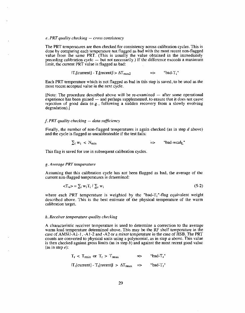
e . PRT quality checking - cross consistency

The PRT temperatures are then checked for consistency across calibration cycles. This is done by comparing each temperature not flagged as bad with the most recent non-flagged value from the same PRT. (This is usually the value obtained in the immediately preceding calibration cycle - but not necessarily.) If the difference exceeds a maximum limit, the current PRT value is flagged as bad:

ITi[current] - Ti[recent]l> ATmax2 => "bad-Ti

Each PRT temperature which is not flagged as bad in this step is saved, to be used as the most recent accepted value in the next cycle.

[Note: The procedure described above will be re-examined - after some operational experience has been gained - and perhaps supplemented, to ensure that it does not cause rejection of good data (e.g., following a sudden recovery from a slowly evolving degradation).]

f . PRT quality checking - data suficiency

Finally, the number of non-flagged temperatures is again checked (as in step d above) and the cycle is flagged as uncalibrateable if the test fails:

Ei wi < Nmin => I'bad-wcalL''

This flag is saved for use in subsequent calibration cycles.

g . Average PRT temperature

Assuming that this calibration cycle has not been flagged as bad, the average of the current non-flagged temperatures is determined:

where each PRT temperature is weighted by the "bad-Ti"-flag equivalent weight described above. This is the best estimate of the physical temperature of the warm calibration target.

h. Receiver temperature quality checking

A characteristic receiver temperature is used to determine a correction to the average warm load temperature determined above. This may be the RF shelf temperature in the case of AMSU-A1-1, -A1-2 and -A2 or a mixer temperature in the case of HSB. The PRT counts are converted to physical units using a polynomial, as in step a above. This value is then checked against gross limits (as in step b) and against the most recent good value (as in step e):

T, < Tmin or T, > Tm, => "bad-T,"

IT,[current] - T,[recent]l > AT,,, => "bad-T,"

29

If the receiver temperature is thus not flagged as bad it is saved for use as the most recent value in the next calibration cycle. For each receiver there is both a primary and a secondary PRT. The processing step described above is performed for both. The secondary reading is used if the primary one fails.

i . Blackbody temperature correction factor

From pre-launch test data a set of table pairs have been determined which relate a warm load (i.e. blackbody) temperature bias to a characteristic receiver temperature, as described above. The first table component is a list of receiver temperatures and the second component is a list of bias values observed at those temperatures. There is a table pair for each channel. The object of this step is to interpolate these tables at the appropriate receiver temperature determined in step h (or in step a ) above. If that temperature has been flagged as bad - or is absent - the most recent accepted value, Tkrecent), is used instead of the current value. (The flag is carried along to indicate that this was done.) The processing is then:

6T,(ch) = interpolate [{T,, 6T,(ch))] at T, (5-3)

The result is one value for each channel. The receiver temperature used in the interpolation (T,) is saved for use in the determination of the calibration coefficients (see 5.5). Note that for AMSU-A channels 9-14 (i.e. for a portion of AMSU-AI-1) there are two redundant PLLO's, each with its own separate 6T correction table. A selector embedded in the telemetry indicates which one of the two is in use.

j . Effective warm load temperature

The final step is to add the bias correction determined in step i to the physical temperature determined in step g :

T,(ch) = <T,> + 6T,(ch) (5-4)

The result is one value for each channel.

5.1.2 Blackbody radiance

a . EfSective radiometric temperature

We account for spectral nonuniformity of the calibration target by making use of a set of predetermined channel-dependent tables of coefficients to transform the target's physical temperature to an effective radiometric temperature. This effect, which accounts for deviations from the otherwise accurate monochromatic assumption, is only significant for channels which cover a relatively wide frequency range, such as the HSB 183-GHz channels. (E.g., for HSB channel 5 the range between the lower edge of the lower sideband and the upper edge of the upper sideband is 16 GHz, i.e. 8.7%.) A linear relationship is assumed. Thus, two coefficients are determined for each channel by lookup in the relevant table:

30

The coefficients are then applied in a linear transformation:

T,'(ch) = bo(ch) + bl(ch)T,(ch) (5-7)

b . Blackbody brightness temperature

The brightness temperature is simply the radiometric temperature determined above times the emissivity, E (which is close to 1):

Tb,(ch) = ET,'(ch) (5-8)

There is one value for each channel, except if the "bad-wcal" flag has been set, in which case Tb, is undefined for all channels.

c . Blackbody radiance

The alternative physical radiance (as described earlier), is determined by applying Planck's function (in wavelength space but in terms of frequencies) to T,':

R,(ch) = E r / [exp(hf/kT,') - 11 (5-9)

where the constant r is defined in terms of Planck's constant, h, and the speed of light, c:

r = 2hf5/c3

and

(5-10)

f the frequency h Planck's constant k Boltzmann's constant c the speed of light

5.1.3 Estimated uncertainties

The uncertainty in Tb, is computed per &. (3-13):

ATbwms(ch) = { [A~T',(ch)]2 + [{ ATb,,fixed}ch]2} 1'2 (5-1 1)

The second term in the expression above represents a table lookup for each channel.

Eq. (5-10) expresses the uncertainty of a single measurement, estimated from a priori system uncertainties and parameters. An equivalent empirical estimate can be made by statistical analysis of the measurements.

31

5.2 Effective Space Brightness

5 2.1 Cosmic background temperature

A value of T, = 2.72 K is used.

5.2.2 Lunar contamination

The moon may occasionally appear within the cold calibration field of view. Due to the polar orbit of the platform, it will always appear to be near the -90" phase, i.e. half-full and waxing. It will then have a brightness temperature of approximately 170-200 K (it appears warmest at the lowest frequencies). Its angular extent is about 0.5". Lunar radiation could therefore be significant against a cold sky background, especially for the narrow-beamed HSB. Furthermore, a "lunar encounter" is likely to last for several calibration cycles, since the spacecraft advances only about 0.16" per HSB cycle relative to the earth (and 0.48" per AMSU-A cycle). Thus, in a worst case, the moon could appear within the half-power beamwidth for about 7 cycles, and significant contamination could last considerably longer.

We will approach this problem by comparing the moon's location relative to the cold calibration field of view with predetermined criteria of significant contamination and set a rejection flag based on the result. Thus, if significant lunar contamination is predicted, the associated cold calibration measurements are simply flagged as bad (i.e. discarded).

This step is implemented in two parts. The first part, which is done as part of the L l a processing, consists of computing the angle between the unit vectors to the center of the moon and the cold space view direction, a . (This is done using the EOSDIS Toolkit.) There is one angle for each AMSU-A scan mirror (i.e. for -Al-1, -A1-2 and -A2) and four angles for HSB, since the HSB scan mirror is not stationary during the consecutive cold calibration samples (unlike AMSU-A). The second part, which is done as part of the L l b processing, consists of comparing the relative lunar angle with precomputed interference limits. The test is

If the "bad-ccal" flag has not been set we proceed with the following steps.

Finally, it should be pointed out that, since lunar 'encounters' are entirely predictable, it may be feasible to avoid the contamination problem by switching to one of the alternate space view positions during the predicted encounter. Although this will result in a discontinuity in the cold calibration time series, that may be preferable to a substantial gap in the data. The initial shakedown period after launch will permit proper characterization of the different space view positions, so that uncertainties can be minimized.

5.2.3 Cosmic-backmound brightness temperature

We use the so-called thermodynamic brightness temperature, which is defined as 21

Tb = (hf/k){[exp(hf/kT) - 11-1 +- 0.5) (5-12)

~ ~~

21 See Aerojet, "Integrated AMSU-A Radiometric Math Model / EOS", Report 10371 (1996) ~~

32

This expression thus relates brightness temperature, Tb, to physical (radiometric) temperature, T. Although this transformation should strictly always be applied, in practice it is only necessary to use it when the physical temperature is very low or the frequency very high. Here it is used for the cold space view only. Thus:

TbCo(ch) = (hf/k){ [exp(hf(ch)/kT,) - 11-l + 0.5) (5-13)

This results in one value for each channel.

5.2.4 Sidelobe correction

To account for radiation from earth received into the antenna sidelobes, both direct and reflected off spacecraft surfaces, as well as radiation from the spacecraft itself, we use a 3-dimensional table relating sidelobe contribution to geographic location (latitude & longitude) and time. There is a table set for each channel, resulting in a channel- dependent sidelobe term. There is a complete set of tables for each allowed cold calibration position (see discussion in 3.2). Initially, a single value per channel will be used, precomputed for each of the four possible space view positions. The computations are based on the measured antenna patterns and a single climatologic average brightness temperature of the Earth for each channel. (For HSB, the actual antenna patterns will not be measured. Instead, the computations will be based on patterns inferred from earlier measurements of AMSU-B antennas.) It is anticipated that the dimensionality and granularity of the sidelobe corrections will be increased after launch based on analysis of actual on-orbit observations. These tables will be updated from time to time. The processing is then:

ATbce(ch) = {GTbSL(Ch)}lat~on,time (5-14)

where k is the cold calibration position index discussed in 3.2. It is used to select the appropriate set of tables. This results in one value for each channel.

5.2.5 Effective space radiance

The total estimated space-view brightness temperature (and the corresponding physical radiance) can now be determined:

Tbc(ch) = Tb,o(ch) + ATbce(ch) (5-15)

and,from Eqs. (5-9) and (5-12),

Rc(ch) = r [kTb,(ch)/hf(ch) - O S ] (5-16)

There is one value for each channel, except if the "bad-ccal" flag has been set, in which case Tb, is undefined for all channels.

5.2.6 Estimated uncertainties

The uncertainty in Tb, is computed per Eq. (3-13):

(5-17)

33

The right-hand side represents a table lookup identical to that of Eq. (5-14).

34

5 3 Radiometric Calibration Counts

Each of the two calibration targets (i.e. the warm load and cold space) is sampled either twice (AMSU-A) or four times (HSB) in rapid succession. The results are digital "counts" which represent the radiometer's output. It is assumed that the radiative environment does not change between successive samplings, so that any differences between the measurements are strictly due to noise - which can be reduced by averaging the measurements.

The procedure described below is identical for both targets. A software implementation would naturally take advantage of that and simply use parameter tables to account for numerical differences, as discussed previously.

5.3.1 Warm load counts

a. Quality check - limits

Each count from each channel is checked against channel-specific gross limits. Those which fall outside the limits are flagged as bad:

Cwi(ch) Cwmidch) or Cwi(ch) > Cwmax(ch) => "bad-wCi(ch)"

Initial values for the gross limits will be supplied by Aerojet. They will be updated based on operational experience, especially during the initial shakedown period after launch.

b. Quality check - self consistency

The counts are next checked for internal consistency. This is done by checking the measurement spread against a channel-specific limit. (An appropriate set of values for these limits will be determined during the initial shakedown period after launch.) The calibration cycle is flagged as bad for any channel which fails this test:

MAX[{Cw(ch)}] - MIN[{Cw(ch)}] > ACwmax(ch) => "bad-wCL(ch)"

where L is the current calibration cycle index.

c . Average counts

We now compute, for each channel, the average calibration count for the current cycle. Thus, for each channel which has not been flagged as "bad-wCL" in step b, we compute the average of the counts which have not been flagged as "bad-wCi" in step a:

(5-18)

where wi(ch) is a particular channel's flag-equivalent binary weight (from step a ) for sample i (i = 1 ..2 for AMSU-A and 1..4 for HSB), as described in 5.1.1.d. This results in one value for each channel, except for those channels which have been flagged as "bad- wCL", which are undefined.

35

5.3.2 Cold space counts

a . 'Quality check - limits

Each count from each channel is checked against channel-specific gross limits. Those which fall outside the limits are flagged as bad:

Cci(ch) < Ccmi,(Ch) or Cci(Ch) > Ccm,,(Ch) => "bad-cCi(ch)"

b. Quality check - self consistency

The counts are next checked for internal consistency. This is done by checking the measurement spread against a channel-specific limit. (An appropriate set of values for these limits will be determined during the initial shakedown period after launch.) The calibration cycle is flagged as bad for any channel which fails this test:

MAX[{CC(ch)}] - MIN[{CC(ch)}] > ACcm,(ch) => "bad-cCL(ch)"

where L is the current calibration cycle index.

e. Average counts

We now compute, for each channel, the average calibration count for the current cycle. Thus, for each channel which has not been flagged as "bad-cCL" in step b, we compute the average of the counts which have not been flagged as "bad-cCi" in step a:

Ccavg~(~h) = Ei wi(ch)Cci(ch) 1 Ei wi(ch) (5-19)

where wi(ch) is a particular channel's flag-equivalent binary weight (from step a ) for sample i (i = 1 ..2 for AMSU-A and 1 ..4 for HSB), as described in 5.1.1 .d. This results in one value for each channel, except for those channels which have been flagged as "bad- cCL", which are undefined.

36

5.4 Smoothed Calibration Counts

.

For the following steps we assume that the preceding steps have been carried forward at least n cycles beyond the current calibration cycle, where n is the parameter referred to below.

5.4.1 Smoothing function

In order to further reduce the measurement noise, the averaged radiometer counts will be smoothed over a number of calibration cycles. This is done by computing a weighted average of the averaged calibration counts of the current cycle, a number (n) of preceding cycles and an equal number (n) of succeeding cycles. A triangular weighting function is used - the current cycle receives a weight of 1 while the weights of preceding and succeeding cycles decline linearly with their distance from the current cycle. Thus, the weighting function is

Wi = 1 - I i I/(n+l) for i = -n .. +n (5 -20)

where i = 0 corresponds to the current cycle. Figure 15 shows an example of W for n = 3, i.e. for 7-point smoothing. An appropriate value for n will be determined during the initial system checkout period after launch.

w

0.25

mi -4 -3 -2 -1 0 1 2 3 4

Figure 15: Smoothing function - example for 7-point smoothing (n = 3)

5.4.2 Smoothed warm load counts

For each channel we compute the weighted average of those cycle averages which have not been flagged as "bad-wCL" in step 5.3.1 .b. Again we use flag-equivalent binary weights, w , to account for the flag conditions (i.e. WL = 0 if "bad-wCL" is set and WL = 1 otherwise).

a. Data suficiency check

We first check if there is enough valid data available to compute a meaningful weighted average. We note that the sum of the smoothing weights is n+l (i.e. if the data from both the current, the n preceding and the n succeeding cycles were available, the total data weight would be n+l). We now require that the sum of the smoothing weights for the available data does not fall below a minimum fraction of the total possible:

37

zi WiwL+i(ch) / (n+l) < XW => "bad-wcalL(ch)"

where i = -n .. +n, xw is the minimum-weight fraction mentioned above, and WL+i(Ch) is the "bad-wC"-flag equivalent weight for the calibration cycle which is offset by i cycles from the current (L) cycle.

b. Weighted average counts

For all channels which passed the test in step a , we can now compute a weighted average:

(5-21)

where Cwavg,~+i is the average warm count for cycle L+i earlier determined in step 5.3.1 .c. There is one value for each channel, except for those channels with the "bad- wcalL" flag set, which are undefined.

5.4.3 Smoothed cold space counts

For each channel we compute the weighted average of those cycle averages which have not been flagged as "bad-cCL" in step 5.3.2.b. Again we use flag-equivalent binary weights, w, to account for the flag conditions (i.e. WL = 0 if "bad-cCL" is set and WL = 1 otherwise).

a. Data suflciency check

We first check if there is enough valid data available to compute a meaningful weighted average. We note that the sum of the smoothing weights is n+l (i.e. if the data from both the current, the n preceding and the n succeeding cycles were available, the total data weight would be n+l). We now require that the sum of the smoothing weights for the available data does not fall below a minimum fraction of the total possible:

zi WiwL+i(ch) / (n+l) < x, => "bad-ccalL(ch)"

where i = -n .. +n, x, is the minimum-weight fraction mentioned above, and WL+i(Ch) is the "bad-cC"-flag equivalent weight for the calibration cycle which is offset by i cycles from the current (L) cycle.

b. Weighted average counts

For all channels which passed the test in step a , we can now compute a weighted average:

where Ccavg,~+i is the average cold count for cycle L+i earlier determined in step 5.3.2.c. There is one value for each channel, except for those channels with the "bad-ccalL" flag set, which are undefined.

38

5.5 Calibration Coefficients

For each channel we will now determine three coefficients, defined in Eqs. (3-7), (3-S), and (3-9) which define the quadratic relationship between brightness temperature and radiometer count described in Eq. (3-3).

5.5.1 Calibration auality flag check

The first step is to check if there is sufficient calibration data to determine a new set of calibration coefficients. If that is not the case, we will use the most recent set of coefficients instead. We proceed as follows:

a . Undefined brightness temperatures - all channels

"bad-wcalL" or "bad-ccalL" => "bad-cal(ch)" for all channels

where the flags originate from 5.1.1 and 5.2.2, respectively.

b . Undefined calibration counts - single channels

"bad-wcalL(ch)" or "bad-ccalL(ch)" => "bad-cal(ch)" for that channel

where the flags originate from 5.4.2 and 5.4.3, respectively.

5.5.2 Nonlinear term

This step may be skipped if the "bad-cal" flag is set for all channels, as in a above. We will assume that the nonlinearity is purely a function of the instrument temperature and that the form of that function remains as it was characterized during pre-launch testing. We use the same instrument temperature that was used in 4.2.1 .i to determine the warm load temperature correction factor, T,. Here, as in that case, we also have a set of table pairs determined from pre-launch test data. The first table component is a list of receiver temperatures and the second component is a list of nonlinearity terms - as defined in Eqs. (3-4) and (3-6) in Section 3 - observed at those temperatures. There is a table pair for each channel. The object of this step is to interpolate these tables at the receiver temperature determined earlier. The nonlinear term is then:

u(ch) = interpolate [{T,, u(ch)}] at T, (5-23)

There is one value for each channel. Note that for AMSU-A channels 9-14 (i.e. for a portion of AMSU-AI-1) there are two redundant PLLO's, each with its own separate ST correction table. A selector embedded in the telemetry indicates which one of the two is in use.

5.5.3 @&

This step is always skipped if the "bad-cal" flag is set for all channels, as in 5.5.1 .a above. We determine the gain for each channel according to the following formula, for all channels which do not have the "bad-cal" flag set:

39

g(ch) = [<Cw(ch)> - <Cc(ch)>] / [Tb,(ch) - Tbdch)] ( 5 -24)

where <C,(ch)> is the smoothed warm load count, from 5.4.2 - Eq. (5-21), cCc(ch)> is the smoothed cold space count, from 5.4.3 - Eq. (5-22), Tb,(ch) is the estimated warm load brightness temperature, from 5.1.2 - Eq. (5-8), and Tbc(ch) is the estimated cold space brightness temperature,from 5.2.5 - E q . (5-15).

5.5.4 Calibration coefficients

a. Good calibration data

For each channel which does not have the "bad-cal" flag (from 5.5.1) set we compute the coefficients as follows (cf. Eqs. (3-7), (3-8) and (3-9)):

a2(ch) = u(ch) / g(ch)2

al(ch) = l/g(ch) - a2(ch) [cC,(ch)> + cC,(ch)>]

*(ch) = Tb,(ch) - cC,(ch)>/g(ch) + a2(ch) cC,(ch)> <C,(ch)>

These values are saved as the most recent coefficients for each channel processed.

b. Bad calibration data

For each channel which has the "bad-cal" flag set we use the most recent coefficients:

ai(ch) = ai(ch)[recent] (5 -25)

fo r i=O . .2 .

6 Computation of Brightness Temperatures

In this section we apply the calibration coefficients determined in Section 5 to all earth scene measurements in a scan cycle (i.e. in a scan line). The results are conventionally called antenna temperatures. We will also apply a correction to reduce the effect of far sidelobe spillover into cold space near the swath edges and near sidelobe smearing of the main beam. The results are then conventionally called brightness temperatures. Finally, we determine certain indices and flags to indicate potential problems with the data.

6.1 Radiometric Calibration

We assume that the calibration coefficients change slowly compared with a scan cycle, so that the coefficients derived from a particular cycle can be applied to all radiometer measurements in that cycle - even though there may be a time lag of up to 2 seconds between scene measurements and the corresponding calibration measurements. (This assumption will be re-examined after launch.)

Then, for each channel (ch) and each scan position (i), the antenna temperatures are, as defined by m. (3-3):

Ta(chj) = ao(ch) + al(ch) C(chj) + a2(ch) C2(chj) (6-1)

where the a's are the calibration coefficients determined in Section 5 for the current scan cycle and the C's are the radiometer counts.

6.2 Far Sidelobe Correction

The example below illustrates the effect we wish to correct for.

Assume for simplicity that the antenna only receives energy through its forward half space, i.e. through a solid angle of 23~; sr. Let us, also for illustrative simplicity, make these further assumptions:

a. The main beam is -8" wide and receives 95% of the energy (i.e. as in

b. The remaining 5% of antenna sensitivity is distributed equally through the

c. The orbit is such that the earth subtends an angle of 130" (i.e. a solid angle

d. The earth has a uniform brightness of 250 K. e. Space has a brightness of 3 K.

AMSU-A).

remaining solid angle (i.e. nearly 23~; sr).

of 1.163~; sr).

When the antenna is pointed towards nadir the earth occupies 1 . 1 6 ~ sr, or a fraction of 0.58 of the available half-space (i.e. 0 .58~5% is received from earth outside the main beam). The radiation received is then as follows:

Main beam (earth) 95% of 250 K = 237.5 K Sidelobes (earth) 2.9% of 250 K= 7.3 K Sidelobes (space) 2.1% of 3 K = 0.1 K

Total radiation received = 244.9 K

41

When the antenna is pointed at 50" away from nadir (at the swath edge), the earth falls partially outside the antenna's forward half space and occupies approximately 0 . 7 8 ~ ~ sr, or a fraction of 0.39 of the available half-space (i.e. 0 .39~5% is now received from earth outside the main beam). The radiation received is now:

Main beam (earth) 95% of 250 K = 237.5 K Sidelobes (earth) 2.0% of 250 K = 4.9 K Sidelobes (space) 3.0% of 3 K = 0.1 K

Total radiation received = 242.5 K

Thus, the asymmetry has resulted in an apparent brightness reduction of 2.3 K.

More precisely, the energy received through the antenna can be expressed as follows:

I T,(Q) A(Q) dS2 + T,(Q) A(Q) dQ carth I space T, =

where

T, is the earth brightness temperature field T, is the cold space brightness temperature A is the antenna pattern SZ is the solid angle variable

We will make the simplifying assumption that T, is constant over the first integral. Eq. (6-2) then simplifies to

T,=(1 -S)T,+ST, (6-4)

where

is the fraction of the antenna pattern which sees cold space rather than the earth.

The true earth brightness temperature can now be estimated:

T, = (T, - ST,) / (1 - S)

For each earth view scan position we will precompute S - one value for each channel, since the antenna pattern varies from channel to channel.

The correction is then computed as follows:

Ta'(chj) = [Ta(chj) - Schj Tb:(ch)] / [l - S,,,J (6-6)

42

where

i is the scan position index (1 ..30 for AMSU-A) ch is the channel index Ta( ch j) is the calibrated antenna temperatures, from E q . (6-1) Tb:(ch) is the cosmic brightness temperature, from Eq. (5-14) S is a table of the space viewing fraction of the antenna pattern

Initially, S will be precomputed from measured antenna patterns. The algorithm, as well as the table, may be updated subsequent to launch, based on analysis of on-orbit observations.

6 3 Near Sidelobe Correction

A deconvolution matrix, in the form of a weight matrix, is pre-computed. Then the antenna pattern correction consists of computing a weighted average of a spatial cluster of measurements centered at scan position I and scan line J:

where Ta’ is the far-sidelobe corrected antenna temperature from Eq. (6-6), i is a scan position offset index, j is a scan line offset index, {d} is the deconvolution weight matrix and {w} is a set of binary weights which ensure that only valid data are used (i.e. w = 1 if the corresponding Ta’ is valid, w = 0 otherwise). There are several versions of the {d} matrix. The primary, symmetric version is used for the majority of scan positions (“interior points”), while special asymmetric versions are used near the swath edges.

Initially, this correction will not be applied.

6.4 Estimated Radiometric Accuracy

We will provide a simple empirical estimate of the radiometric accuracy, NEDT, for each channel. For each calibration cycle we compute an estimate of the rms of the fluctuations in the consecutive calibration measurements (i.e. counts) for each channel. For AMSU-A, this is simply the difference between two consecutive readings divided by the square root of 2, while for HSB we will use the root-sum-squared average of three consecutive such differences. The result is then transformed to brightness temperature units (K) by dividing by the gain, g. (We ignore nonlinearities in this context.) These per-scanline estimates are then root-sum-squared to form longer term (and more stable) estimates.

6.5 Estimated Calibration Accuracy

We determine the calibration accuracy for each channel per Eq. (3-10). Substituting brightness temperatures, we get

ATb,,l(chj) = {[X ATb,P + [( 1-X) ATb$ + [4(X-X2) ATbNd2 + [ATb,,J2}1’2 (6-8)

where

43

x = (Ta(chj) - Tb,)/(Tb, -Tb,)

ATb, = ATbWms@h) from Eq. (5-1 1)

ATb, = ATbCms(ch) from E q . (5-18)

ATbNL = {ATbNL(ch)},h table lookup of the peak nonlinearity

ATb,,, = {ATbsys(ch)},h table lookup of the system uncertainty

This results in one value per channel for each earth scene. Note that this, unlike the estimate discussed in 6.4, is not an empirical estimate but rather represents an expectation value based on known instrument characteristics and the radiometric environment. Also, the procedure described in 6.4 yields one channel set per scan line, while the procedure described here yields one channel set per footprint.

6.6 Sun glint

The Earth's surface can be quite reflective (ocean reflectivity can exceed 0.5 at some microwave frequencies), as well as scattering. Therefore, there will be both specularly reflected and scattered solar radiation coming from the surface. Since the brightness temperature of the sun is on the order of 10,000 K, this can result in substantial microwave radiation at viewing angles close to the direction of specular reflection.

Whether this becomes a problem depends on the orbit. The design orbit for EOS-PM1 is a sun synchronous orbit with a 1 :30 PM ascending node and an inclination of about 98". Thus, the sun's longitude at the spacecraft's northbound equator crossing is 22.5" west of the subsatellite point (nadir). At the equator, the microwave instruments scan out to about 8" west of the nadir point (a 49" nadir angle from a 705-km altitude) and about 1" south (due to the inclination of the orbit). Within the scan swath the solar angle of incidence will increase from about 14.3" (at the swath edge) to 22.3" (at nadir). On the other hand, the instrument's viewing angle of incidence increases from 0" (at nadir) to 57" (at the swath edge). Somewhere within the western half of the swath there must therefore be a point where the two angles of incidence are equal and specular reflection results. For the EOS-PM1 orbit this will happen at approximately 3" west of nadir, or at a nadir scan angle of approximately 17", where the angle of incidence is about 20". (These angles are only approximate and will change with the season.) It is certain, however, that specular reflection conditions will exist once per orbital revolution (namely, approximately 3" north of the crossing of the plane of the ecliptic 22).

The relevant surface properties are very variable and unpredictable. We will therefore approach this problem in a purely geometric sense, by computing a sun glint "proximity index" for each scan position. This index, which is proportional to the inverse of the distance between a footprint and the sun glint spot, will be a measure of the likelihood of sun glint effects. The user must apply surface information and must be aware of the masking effect of high atmospheric opacity. (It is only relatively transparent channels that might be affected by sun glint.)

22 At the equinoxes, the subsolar point is on the equator and 22.5" west of the ascending node. With an orbital inclination of 98", the subsolar point would then be in the scan plane when the subsatellite point is approximately 3" north of the equator. In general, the subsolar point will appear in the scan plane when the subsatellite point is about 3" north of the ecliptic. This value varies slightly with the season.

44

The EOSDIS Toolkit is used to determine the location of the sun glint for each scan position. Its distance from the center of the footprint on the surface is then computed, and finally the ratio between a predetermined scale length and the sun glint distance is truncated to an integer valued sun glint index. If the index has a high value, indicating a high likelihood of sun glint contamination of surface channels, a flag is set. Thus, the steps are, for each footprint

1 . Compute latitude and longitude of the sun glint spot (if any) 2. Compute the distance between footprint center and the sun glint spot, d-glint 3. Compute glint-index = L-glintld-glint 4. Set the flag: If glint-index > glint-crit => “possible glint”

L-glint and glint-crit are predetermined parameters, which will be updated after launch.

It is expected that this algorithm, as well as the parameters, will be updated subsequent to launch, based on analysis of on-orbit observations.

6.7 Coast Contamination

While the AMSU-A “beam width” is approximately 3.3”, a significant fraction of the radiation received comes from outside this 3-dB beam. Thus, about 95% of the energy comes from the so-called main beam, which is more than 8” wide. The effect of this is to smear out sharp edges in the observed field. This is particularly the case at coast lines, where the emissivity may sudenly jump by more than 0.5 in some channels. Thus, the brightness temperature might be 150 K over the ocean and jump to 300 K over land. The wide and “fuzzy” beam will smear out the resulting 150 K step and make it noticeable far away from the coast itself. Unless accounted for, this can result in large errors. (The smearing effect is also significant for HSB, but it is less due to a narrower and more efficient main beam.)

The purpose of the coast contamination algorithm is twofold: to indicate to the user that there is likely coastal contamination in some channels, and to provide a quantitative estimate of its magnitude which can be used in downstream (L2) corrective processing. This algorithm is still under development, but the intention is to provide a “beam weighted” land/ocean fraction which will indicate how much of the received radiation originates from an ocean surface (vs. land) to a sufficient accuracy that it can be used in the retrieval processing to compensate for the blurring effect without unduly amplifying the effective measurement noise. A user flag will be derived from this fraction. Without the ability to compensate for such contamination, a measurement thus flagged would have to be rejected from further processing.

6.8 Quality Assessment

A number of flags and other indicators will be used to alert the user to potential problems and in general indicate the estimated quality of the calibration process and its results. This will not be discussed in detail here (a separate QA Plan is under development, where the subject will be discussed in detail), but we will provide a summary here. Quality Assessment parameters are provided at several data granularities: at the swath file level (the “granule” in EOSDIS nomenclature - in the current design this consists of 45 AMSU-A scan lines or 135 HSB scan lines), at the scan line level (i.e. per calibration

45

.

cycle), and at the footprint level. Most of the quality assessment is generated at the scan line level and presented to the user along with the primary data parameters per scan line. Most of these parameters are then summarized at the “granule” level. Some of them are further summarized on a daily basis in a browse product.

The QA parameters fall into the following categories Quality of the input data per L la processing QA Quality of the input data per L l b data testing Quality of the calibration processing steps Error estimates Problem indicators not related to calibration processing

Appendix B contains a list of currently baselined QA parameters. (It should be noted that this area is under development, however.)

In addition to such QA parameters, every data product (e.g., calibrated brightness temperatures) will have error estimates associated with it. The algorithms discussed in preceding sections include descriptions of how such error estimates are derived.

7 Post-Launch Verification and Validation

I

Soon after launch the instruments will be activated and their performance analyzed and compliance with required performance verified. In particular, all L lb data products will be validated, with emphasis on the radiometric performance.

7.1 Radiometric Validation

This subject is discussed in detail in the AIRS Validation Plan23 and will only be summarized here.

Three techniques will be used to validate the microwave radiances (brightness temperatures):

Vicarious calibration, where a well known (and usually radiometrically simple) radiating target is viewed. An example is viewing the moon. Cross-validation, where comparisons are made with the radiances obtained with another instrument with similar characteristics viewing an identical air mass. An example is comparisons between AMSU-A and AMSR-E, which have one spectral channel in common. In situ measurements, where residuals between radiances computed from measured geophysical observations and observed radiances are analyzed. An example is observations over one of the DOE’S ARMKART sites, where intensive field observations are obtained with multiple instrument packages, including both ground and airborne sounders, while the spacecraft passes above.

It will also be possible to validate radiometric performance indirectly, by analyzing climatology (i.e. long term averages) derived from the instrument observations and comparing that with values obtained from other sources.

7.2 Spatial Calibration

Although the so-called geolocation processing is part of Lla , we will discuss the validation (and calibration) of the instrument pointing here. The algorithms described in this section are not implemented in the automated data processing system (EOSDIS/DAAC/PGS) but will be implemented at the TLSCF as part of the occasional processing which will take place there. They are merely described here for completeness.

Three methods are envisioned to check the absolute and relative pointing accuracies. The first method consists of commanding the instrument into stare mode - where the scan is suspended while the antenna is indefinitely pointed towards nadir. The object is to detect a sharp edge in the radiative scene, such as one due to a coastline or an ice edge. The second method compares results from AIRS with those from the microwave instruments, for spatial cross-correlation. The third method depends on analysis of surface maps generated from long time series.

7.2.1 Surface edge crossings - Stare mode

E. Fetzer (ed.): “AIRS Validation Plan”, NASAIJPL #D-16822 (1999)

47

In stare mode the antenna is locked in the position nearest the nadir direction. It remains there until commanded otherwise. Although no calibration measurements are taken during this time, the data control system still follows the normal measurement pattern - i.e. for AMSU-A a 6-second scene observation period with 30 earth views is followed by a 2-second blank interval. The sampling of the nadir scene is therefore dense but has regular gaps.

This mode can be used to calibrate the antenna pointing, as well as to estimate the antenna pattern, in two orthogonal directions: alongtrack and crosstrack. For alongtrack calibration, the crossing of a coast line which is nearly in the crosstrack direction is used. The emissivity difference between water and land will cause a shift in the radiance measured by the most transparent channels, which can be used to estimate the exact time of crossing. A comparison with surface maps will then allow the alongtrack pointing angle to be determined to good accuracy.

For crosstrack calibration an oblique coastal crossing is used, i.e. where the coast line is nearly (but not exactly) parallel to the sub satellite track. The angle and length must be sufficient that the coast line sweeps through the field of view.

It may also be possible to use ice-water edges, which can provide even higher contrast than land-water edges, if the location of the edge can be ascertained with sufficient accuracy.

Finally, it is also possible to use the moon for spatial calibration, since the microwave instruments also allow a space calibration position stare mode, where the antenna is frozen in one of the space view positions. This could be done on occasions when the moon is predicted to move through the field of view. (See 5.2.2 for a related discussion.)

7.2.2 Cross-calibration with AIRS

While the method described above provides absolute spatial calibration, it is also possible to obtain relative calibration between AIRS and the microwave instruments. If the instruments are perfectly coregistered, surface features with substantial contrast will appear in the fields of view simultaneously. By accounting for the time lags associated with the different scan speeds and the angles between the respective scan planes, it is possible to determine the pointing angle differences.

7.2.3 Long term surface map analysis

This method is similar to the method described in 7.2.1. However, it relies on the permanence of surface features (such as coast lines). It consists in eliminating sampling uncertainty by determining long term averages of measured coastal crossings. While individual samplings have large uncertainties due to the size of the field of view as well as the low sampling density, long term averages will have increasingly high accuracy. The coast maps thus generated can then be compared with geodetic maps.

A detailed discussion of this approach can be found in the AIRS Level l b Part 2 ATBD (IWVIS).

48

#

Appendix A: Quality Assessment Parameters (draft)

The following is a draft list of currently baselined QA parameters. Note that this is a drup only. It will be revised and finalized well before launch.

The following parameters are used below: c: number of channels (15 for AMSU-A, 4 for HSB) i: number of instrument modules (2 for AMSU-A, 1 for HSB) r: number of receivers (3 for AMSU-A, 1 for HSB) s: number of Earth scene scan positions (30 for AMSU-A, 90 for HSB)

Per Pranule

Number of scan lines in this granule Number of scan lines in this granule not in normal scan mode Number of calibrated scan lines in this granule Number of missing scan lines in this granule Number of data gaps in this granule Number of instrument mode changes in this granule Number of scan lines with calibration problems - per receiver Number of scan lines with calibration problems - per channel Number of scan lines with significant coast contamination Number of scan lines with significant sun glint Input radiometer scene count statistics for this granule Input radiometer calibration count statistics for this granule (warm & cold) Input blackbody temperature statistics for this granule (all PRTs) Input receiver temperature statistics for this granule (all PRTs) Calibration coefficient statistics for this granule Blackbody “raw” noise count statistics for this granule Space view “raw” noise count statistics for this granule NEDT estimate statistics for this granule Ratio of NEDT-estimate to NEDT-nominal statistics for this granule

[ 1 *Int] [i*Int] [r*Int] [i*Int] [i*Int] [i*Int] [r*Int] [c*Int] [ 1 *Int] [ 1 *Int]

[s*c*UES] [2*c*UES]

[r*LES] [r*LES]

[c*3*UES] [c*UES] [c*UES] [c*UES] [c*UES]

Per scan line

Calibration problem summuryflug - for each receiver [r*Byte] Bit Meaning 7

This scan line was calibrated, but some PRT values were bad or marginal 5 This scan line was calibrated, but there was a data gap 6 Some channels were not calibrated

’ 4 This scan line was calibrated. but there was a blackbodv scan Dosition error I 3 I This scan line was calibrated. but there was a mace view scan Dosition error I

2

This scan line was not calibrated, due to the instrument mode 0 This scan line was not calibrated, due to bad or missing PRT values 1 This scan line was calibrated, but the moon was in the space view

49

Calibration qualityflags - for each channel [c*Byte] Bit Meaning 7

Most recent calibration coefficients used 6 Excessive NEDT estimated

5

2 All blackbody counts were bad for this channel and scan line 3 Blackbody counts were marginal for this channel and scan line 4 Blackbody counts could not be smoothed

All space view counts were bad for this channel and scan line 0 Space view counts were marginal for this channel and scan line 1 Space view counts could not be smoothed

~ ~ ~ _ _ _ _

Non-calibration indicators [ 1 *Byte] Bit I Meaning 7 1 6 5 4 3 I Near sidelobe correction applied 2 I Some channels had excessive NEDT estimate 1 I Coastal contamination in this scan line 0 I Sun glint in this scan line I

Per footprint

None

50