aircraft impacts on local and regional air quality in the

Partnership for AiR Transportation Noise and Emissions ReductionAn FAA/NASA/Transport Canada-sponsored Center of Excellence

Aircraft Impacts on Local and Regional Air Quality in the United States

PARTNER Project 15 final report

prepared by

Gayle Ratliff, Christopher Sequeira, Ian Waitz, Melissa Ohsfeldt, Theodore Thrasher, Michael Graham, Terence Thompson

October 2009

REPORT NO. PARTNER-COE-2009-002

Aircraft Impacts on Local and Regional Air

Quality in the United States

Partnership for AiR Transportation Noise And Emissions Reduction Project 15 Final Report

Gayle Ratliff, Christopher Sequeira, and Ian Waitz Massachusetts Institute of Technology, Cambridge, Massachusetts

Melissa Ohsfeldt and Theodore Thrasher CSSI Inc, Washington DC

Michael Graham and Terence Thompson

Metron Aviation, Herndon, Virginia

PARTNER-COE-2009-002 October 2009

This work was funded by the U.S. Federal Aviation Administration Office of Environment and Energy under DTFAWA–05-D-00012, Task Order No. 0003. The project was managed by Dr. Warren Gillette.

Any opinions, findings, and conclusions or recommendations expressed in this material are those of the authors and do not necessarily reflect the views of the FAA, NASA or Transport Canada.

The Partnership for AiR Transportation Noise and Emissions Reduction — PARTNER — is a cooperative aviation research organization, and an FAA/NASA/Transport Canada-sponsored Center of Excellence. PARTNER fosters breakthrough technological, operational, policy, and workforce advances for the betterment of mobility, economy, national security, and the environment. The organization's operational headquarters is at the Massachusetts Institute of Technology.

The Partnership for AiR Transportation Noise and Emissions Reduction Massachusetts Institute of Technology, 77 Massachusetts Avenue, 37-395

Cambridge, MA 02139 USA http://www.partner.aero

[email protected]

1

Table of Contents

1 EXECUTIVE SUMMARY ...................................................................................................................... 9 2 OVERVIEW OF STUDY AND REPORT ORGANIZATION ................................................................ 15 3 THE IMPACT OF AIRCRAFT EMISSIONS ON NONATTAINMENT AREA, LOCAL, AND REGIONAL AIR QUALITY AND PUBLIC HEALTH ................................................................................. 17

3.1 CREATION OF A BASELINE INVENTORY.......................................................................................... 18 3.2 IMPACT OF AIRCRAFT EMISSIONS ON AMBIENT AIR QUALITY.......................................................... 39 3.3 THE IMPACT OF AIRCRAFT EMISSIONS ON PUBLIC HEALTH ............................................................ 43 3.4 LEAD EMISSIONS FROM PISTON ENGINE AIRCRAFT ....................................................................... 48

4 OPPORTUNITIES TO ENHANCE FUEL EFFICIENCY AND REDUCE EMISSIONS: BENEFITS OF REDUCING AIRPORT DELAYS............................................................................................................... 50

4.1 THE RELATIONSHIP BETWEEN DELAY AND EMISSIONS ................................................................... 50 4.2 POTENTIAL BENEFITS FROM REDUCED GROUND DELAYS .............................................................. 55

5 WAYS TO PROMOTE FUEL CONSERVATION: INITIATIVES AIMED AT IMPROVING AIR TRAFFIC EFFICIENCY ............................................................................................................................. 58

5.1 AIRSPACE FLOW PROGRAMS IN SUPPORT OF SEVERE WEATHER AVOIDANCE PROCEDURES........... 61 5.2 SCHEDULE DE-PEAKING.............................................................................................................. 62 5.3 CONTINUOUS DESCENT ARRIVALS ............................................................................................... 64 5.4 NEW RUNWAYS AND RUNWAY EXTENSIONS.................................................................................. 65

6 CONCLUSIONS AND RECOMMENDATIONS .................................................................................. 67 7 REFERENCES.................................................................................................................................... 70 APPENDIX A STUDY PARTICIPANTS................................................................................................. 72 APPENDIX B STUDY AIRPORTS......................................................................................................... 73 APPENDIX C PM METHODOLOGY DISCUSSION PAPER................................................................. 84 APPENDIX D DATA COLLECTION AND ANALYSIS OF AIRCRAFT AUXILIARY POWER UNIT USAGE 98 APPENDIX E EMISSIONS AND DISPERSION MODELING SYSTEM (EDMS) BASELINE AIRCRAFT EMISSIONS INVENTORY....................................................................................................................... 102 APPENDIX F MODELING OF THE IMPACT OF AIRCRAFT EMISSIONS ON AIR QUALITY IN NONATTAINMENT AREAS.................................................................................................................... 106 APPENDIX G HEALTH IMPACT FUNCTIONS AND BASELINE INCIDENCE RATES ..................... 162 APPENDIX H LIST OF COUNTIES BY PM MORTALITY................................................................... 170 APPENDIX I EMISSIONS REDUCTIONS AT 113 AIRPORTS DUE TO ABSENCE OF GROUND DELAYS 171 APPENDIX J COMPARISON OF EDMS AIRCRAFT EMISSIONS WITH OTHER SECTORS IN THE 2002 NEI -- FOR NAAS........................................................................................................................... 176

2

LIST OF TABLES

Table 1.1: Contribution of aircraft LTO operations at commercial service, reliever, and general aviation airports with commercial activity to emissions inventoriesa,b,c,d ............................................................................................... 10

Table 1.2: NAA Annual NOx Emission Levels for Mobile and Other Source Categories for 2002 (148 Commercial Service Airports)a, b, c, d, e...................................................................................................................................... 11

Table 3.1: List of nonattainment areas with at least one commercial service airport, as of September 7, 2005a ........ 23 Table 3.2: Contribution of U.S. aircraft LTO operations at 148 commercial service airports to emission inventories in

118 NAAs a, b, c, d.................................................................................................................................................. 30 Table 3.3: Top 25 NAAs according to aircraft PM2.5 contribution ................................................................................. 31 Table 3.4: Top 25 NAAs according to aircraft NOx contribution ................................................................................... 32 Table 3.5: Aircraft emissions contribution for top 25 NAAs according to LTOs (NOx, VOCs, and PM2.5)................... 33 Table 3.6: Aircraft emissions contribution for top 25 NAAs according to population (NOx, VOCs, and PM2.5)............. 34 Table 3.7: Nonattainment area annual NOx emission levels for mobile sources(metric tons)a,b,c,d .............................. 36 Table 3.8: Nonattainment area annual PM2.5 emission levels for mobile sources (metric tons)a,b,c,d ........................... 36 Table 3.9: Contribution of aircraft LTO operations at commercial service airports to emissions inventories ............... 37 Table 3.10: Average annual PM2.5 estimates. Results are given in µg/m3. The annual National Ambient Air Quality

Standard for PM2.5 is 15.0 µg/m3. ....................................................................................................................... 40 Table 3.11: Average 8-hour ozone values (ppb) with and without EDMS aircraft emissions. The National Ambient Air

Quality Standard for 8 hour ozone is 80 ppb. Based on rounding convention, values greater than or equal to 85 ppb are considered non-attainment. ................................................................................................................... 42

Table 3.12: Health effects due to aircraft emissions, continental United States. ......................................................... 44 Table 3.13: Ten counties with highest PM-related mortality incidences....................................................................... 46 Table 4.1: Emissions reductions at selected airports with no ground delay................................................................. 57 Table 5.1: Reduction in emissions and fuel burn due to the implementation of AFPs instead of GDPs at Boston Logon

and Chicago O'Hare airports............................................................................................................................... 62 Table 5.2: Estimated reductions from schedule de-peaking ........................................................................................ 63 Table 5.3: Emissions and fuel burn percentage reductions relative to the baseline below 3,000 feet, comparing five

levels of CDA usage to the baseline for all modeled approaches to LAX (Dinges 2007). .................................. 64 Table 5.4: Table of percentage reduction in fuel burn and emissions achieved by applying the 2006 taxi out time to

the 2005 flights for an effective 15% reduction in taxi-out time........................................................................... 65 Table 5.1: Summary of emissions reductions potential from operational initiatives ..................................................... 66 Table C.1: Assumed Average Air-to-Fuel Ratios by Power Setting ............................................................................. 85 Table C.2: Derived “Non_S_Component values by mode [mg/kg fuel] ........................................................................ 90 Table C.3: Computed standard deviations for the volatile PM component .................................................................. 91 Table C.4: ICAO fuel use rates for three engines evaluated. [kg/s] ............................................................................. 93 Table C.5: Total fuel use for climbout and takeoff modes [kg fuel] .............................................................................. 93 Table C.6: Lubrication oil EIs for climbout and takeoff for selected engines. [mg/kg fuel] ........................................... 94 Table D.1: APU use per LTO cycle (minutes) ............................................................................................................ 100 Table F.1: Vertical layer structure for MM5 and CMAQ (heights are layer top). ........................................................ 109 Table F.2: Ratios of EDMS emissions to overall base line (scenario #2) emissions averaged nationally, and for the 12

cities with the largest modeled PM2.5 impact from EDMS aircraft emissions. ................................................. 112 Table F.3: Annual CMAQ 2001 model performance statistics for 2001 base case (scenario #1).............................. 113

3

Table F.4: CMAQ 8-hourly daily maximum ozone model performance statistics calculated for a threshold of 60 ppb over the entire 36 km domain for 2001. ............................................................................................................ 114

Table F.5: CMAQ 8-hourly daily maximum ozone model performance statistics (NMB and NME) calculated for specific subdomains and using a threshold of 60 ppb over the entire domain for 2001. ................................. 114

Table F.6: Average projected PM2.5 design values over the U.S. for the base line (scenario #2) and the two modeling scenarios #3 and #4 (no aircraft emissions, and with EDMS aircraft emissions, respectively). Units are µg/m3........................................................................................................................................................................... 117

Table F.7: For the 37 existing PM2.5 nonattainment areas, model-estimated PM2.5 design values for scenarios #4 and #3, along with average ambient FRM design values. Units are µg/m3. ........................................................... 117

Table F.8: Average projected 8-hour ozone design values for primary strategy modeling scenario. Units are ppb. 120 Table G.1: Health impact functions used in BenMAP to estimate benefits of PM reductions .................................... 163 Table G.2: Health impact functions used in BenMAP to estimate benefits of ozone reductions................................ 165 Table G.3: Baseline incidence rates used in BenMAP for the general population ..................................................... 166 Table G.4: Asthma prevalence rates used in BenMAP .............................................................................................. 167 Table J.1: Nonattainment area annual NOx emission levels for mobile source categories for 2002 a,b,c,d. Units are

metric tons. ....................................................................................................................................................... 176 Table J.2: Nonattainment area annual PM2.5 emission levels for mobile source categories for 2002. Units are metric

tons. .................................................................................................................................................................. 177 Table J.3: Nonattainment area annual VOC emission levels for mobile source categories for 2002. Units are metric

tons. .................................................................................................................................................................. 177 Table J.4: Nonattainment area annual CO emission levels for mobile source categories for 2002. Units are metric

tons. .................................................................................................................................................................. 178 Table J.5: Nonattainment area annual SO2 emission levels for mobile source categories for 2002. Units are metric

tons. .................................................................................................................................................................. 178

4

List of Figures

Figure 2.1: Organization of this study........................................................................................................................... 15 Figure 3.1: Commercial service airports located in ozone, PM2.5, CO, PM10, NO2, and SO2 nonattainment areas in

2005. ................................................................................................................................................................... 18 Figure 3.2: 148 Nonattainment airports and the additional 177 modeled for the study................................................ 20 Figure 3.3: Overview of EDMS inputs .......................................................................................................................... 21 Figure 3.4: Estimated change in annual PM2.5 concentrations (µg/m3) due to aircraft emissions. ............................... 41 Figure 3.5: Estimated change in 8-hour ozone concentrations (ppb) due to aircraft emissions. Negative values

represent regions where aircraft emissions reduce levels of ozone. Positive values represent regions where the aircraft emissions increase ozone levels. ........................................................................................................... 42

Figure 4.1: Taxi-Out Emissions of Boeing 737s at ATL Mapped to their Corresponding Taxi-Out Time. Grams of pollutant per operation are normalized by the mass of the aircraft in metric tons............................................... 52

Figure 4.2: Average carbon monoxide (CO) and NOx emissions per operation as function of time of day for Boeing 737 aircraft at ATL averaged over the period between November 15th and December 27th, 2005. Increased emissions are found around 9 o’clock in the morning and between 4pm and 8pm in the evening, corresponding with increases in taxi out times. This pattern of delay and emissions is related directly to the increases in the number of departure operation during these times. ............................................................................................ 53

Figure 4.3: Average carbon monoxide (CO) and NOx emissions per operation as function of time of day for CRJ-200 aircraft at PHF averaged over the period between November 15th and December 27th, 2005. There is a consistent range of taxi out times between 10 and 15 minutes with the exception of three hours of operation. At noon there was only one operation. The delays at 8:00 PM are unlikely to be the result of congestion since the capacity at this airport is 55 operations per hour and during these two hours of the day only 32 aircraft departed over the six-week period. Congestion at other destinations likely delayed flights from PHF. ............................. 54

Figure 4.4: Average carbon monoxide (CO) and NOx emissions per operation as function of time of day from Boeing 737’s at EWR averaged over the period between November 15th and December 27th, 2005. This delay pattern is more indicative of the departure demand generally exceeding the available departure capacity for the airport, with the exception of the time period between 4:00 AM and 6:00 AM, where the taxi-out times are below 20 minutes and very few flights depart relative to the rest of the day. ..................................................................... 55

Figure 4.5: Percentage savings in LTO fuel use with the absence of ground delays at the 113 selected airports. With fewer operations and less fuel consumed, smaller airports are able to achieve large percentage changes when comparing the operational baseline to the no delay scenario. While at larger airports with more delay and operations, small percentage changes in the fuel consumption result in large quantities of fuel saved............. 56

Figure 4.6: Metric tons of fuel saved with the absence of ground delays for the 113 selected airports ....................... 56 Figure 5.1: Taxi-out times for Cleveland Hopkins Airport (CLE) during the month of April 2005. ................................ 60 Figure 5.2: Hourly minutes of delay at BOS (left) and ORD (right) during the afternoon of April 20, 2005 compared to

average minutes of delay for the entire month of April 2005. Bad weather brought delays resulting in longer taxi out times during the afternoon hours. ................................................................................................................. 62

Figure 5.3: Original and modified hourly taxi-out times for PHX are based on monthly average for April 2005 (estimated unimpeded time of 8 minutes)........................................................................................................... 63

Figure 5.4: Baseline downwind approaches at LAX from Dinges, 2007. ..................................................................... 64 Figure C.1: Trends from APEX 1 for CFM56-2-C1 engine........................................................................................... 89 Figure C.2: Comparison of FOA3.0a to FOA 3.0 for the PW4158 engine.................................................................... 95 Figure C.3: Comparison of FOA3.0a method to FOA 3.0 for the CFM56-3B-2 engine. ............................................... 95 Figure C.4: Comparison of FOA3.0a method to FOA 3.0 for the RB211-535E4 engine.............................................. 96 Figure C.5: Comparison of FOA3.0a method to FOA 3.0 for the GE90-77B engine.................................................... 97 Figure D.1: Range of the percentage of aircraft emissions due to APU at 325 airports studied ................................ 101 Figure E.1: Overview of the generation of the baseline inventory.............................................................................. 103 Figure F.1: Map of the CMAQ modeling domain. The box outlined in black denotes the 36 km modeling domain. . 108

5

Figure F.2: Model-projected impacts of removing EDMS emissions on annual PM2.5 design values. Units are µg/m3. Negative values indicate annual PM2.5 levels would be lower without the aircraft emissions contribution. ...... 119

Figure F.3: Model-projected impacts of removing EDMS emissions on annual average PM2.5. Units are µg/m3. Negative values indicate annual PM2.5 levels would be lower without the aircraft emissions contribution. ...... 120

Figure F.4: Model-projected impacts of removing EDMS emissions on 8-hour ozone design values. Units are ppb. Negative values indicate annual ozone levels would be lower without the aircraft emissions contribution. Positive values indicate that the inclusion of EDMS aircraft emissions suppresses average ozone levels...... 122

Figure F.5: Model-projected impacts of removing EDMS emissions on July average ozone. Units are ppb. Negative values indicate monthly average ozone levels would be lower without the EDMS aircraft emissions contribution. Positive values indicate that the inclusion of EDMS aircraft emissions suppresses average ozone levels...... 123

6

List of Acronyms

µg/m3 Micrograms per Cubic Meter

AFP Airspace Flow Program

APU Auxiliary Power Unit

ASDE-X Airport Surface Detection Equipment, Model X

ASPM Aviation System Performance Metrics

ATADS Air Traffic Activity Data System

ATM Air Traffic Management

Avgas Aviation gasoline

BenMAP Environmental Benefits Mapping and Analysis Program

BTS Bureau of Transportation Statistics

CAEP ICAO Committee on Aviation Environmental Protection

CAFE Clean Air for Europe

CAIR Clean Air Interstate Rule

CAVS CDTI Assisted Visual Separation

CDA Continuous Descent Arrivals

CDTI Cockpit Display of Traffic Information

CFR Code of Federal Regulations

CMAQ Community Multi-Scale Air Quality Modeling System

CO Carbon Monoxide

CO2 Carbon Dioxide

COPD Chronic Obstructive Pulmonary Disease

CSC Computer Sciences Corporation

DFM Departure Flow Management

DSP Departure Spacing Programs

EAC Early Action Compact

7

EDMS Emissions and Dispersion Modeling System

EPA U.S. Environmental Protection Agency

ETMS FAA Enhanced Traffic Management System

FAA Federal Aviation Administration

FIPS Federal Information Processing Standard

FMS Flight Management System

FOA First Order Approximation

FOA3 First Order Approximation version 3.0

FOA3a First Order Approximation version 3.0a

GA General Aviation

GDP Ground Delay Program

GPS Global Positioning System

HAP Hazardous Air Pollutant

HC Hydrocarbons

HO2 Hydroperoxyl radical

IFR Instrumental Flight Rules

ITWS Integrated Terminal Weather System

LTO Landing Take-Off

MIT Massachusetts Institute of Technology

MRAD Minor Restricted Activity Days

NAA NonAttainment Area

NAAQS National Ambient Air Quality Standards

NAS National Airspace System

NASA National Aeronautics and Space Administration

NASR National Airspace System Resources

NEI National Emissions Inventory

NMHC Non-Methane Hydrocarbon

NOx Oxides of Nitrogen

8

NPIAS National Plan of Integrated Airport Systems

OEP Operational Evolution Partnership

OH Hydroxyl radical

PARTNER Partnership for AiR Transportation Noise and Emissions Reduction

PM Particulate Matter

PM10 Particulate Matter less than 10 µm in diameter

PM2.5 Particulate Matter less than 2.5 µm in diameter

ppb Parts per billion

ppm Parts per million

PRM Precision Runway Monitor

RIA Regulatory Impact Analysis

RNAV Area Navigation

RNP Required Navigation Performance

SAGE FAA System for Assessing Aviation’s Global Emissions

SI Spark Ignition

SIP State Implementation Plan

SOx Oxides of Sulfur

SWAP Severe Weather Avoidance Procedures

TAF Terminal Area Forecast

THC Total Hydrocarbon

TSD Technical Support Document

VALE Voluntary Airport Low Emissions Program

VFR Visual Flight Rules

VOCs Volatile Organic Compounds

9

1 Executive Summary This report documents the findings of a study undertaken to identify:

The impact of aircraft emissions on air quality in nonattainment areas (NAAs); Ways to promote fuel conservation measures for aviation to enhance fuel efficiency and reduce emissions;

and Opportunities to reduce air traffic inefficiencies that increase fuel burn and emissions.

This study was conducted by the Partnership for AiR Transportation Noise and Emissions Reduction (PARTNER), an FAA/NASA/Transport Canada-sponsored Center of Excellence. Appendix B contains the full list of study participants. The study was conducted through the coordinated efforts of five contractors and subcontractors.

Aircraft landing take-off (LTO) emissions include those produced during idle, taxi to and from terminal gates, take-off and climb-out, and approach to the airport. Aircraft LTO emissions contribute to ambient pollutant concentrations and are quantified in local and regional emissions inventories. This study analyzed aircraft LTO emissions at 325 airports with commercial activity (including 263 commercial service airports and 62 airports that are either reliever or general aviation airports) in the U.S for operations that occurred from June 2005 through May 2006. The flights studied represent 95% of the aircraft operations for which flight plans were filed during that time period (and 95% of the operations with International Civil Aviation Organization (ICAO) certified jet engines in the U.S.). Of the 325 airports, 148 are commercial service airports in ambient air quality nonattainment areas as specified by the National Ambient Air Quality Standards (NAAQS) (40 CFR Part 50). The airports involved are identified in Appendix B; the nonattainment areas are listed in Table 3.1. Each of these NAAs has at least one commercial service airport.

The study was designed to focus on the impact of aircraft emissions on air quality in NAAs. As is shown in Table 1.1, aircraft operations at the 148 commercial service airports in the 118 NAAs are less than 1 percent of emissions in these areas. Aircraft emissions data from 2005 were used for this study. In the table, non-aircraft emissions data are from EPA’s year 2002 National Emissions Inventory. Note that EPA’s year 2001 National Emissions Inventory was used for modeling the impact of aviation emissions on air quality and human health; see section 3.1 for details. (Note, some of the general aviation airports and reliever airports studied were located in NAAs, but they were not included with the below inventories for NAAs. The aircraft emissions from these airports are estimated to be a small fraction of the aircraft emissions in NAAs compared to those from commercial service airports because commercial aircraft are generally larger than general aviation aircraft and thus burn more fuel; emissions are proportional to fuel burn.)

10

Table 1.1: Contribution of aircraft LTO operations at commercial service, reliever, and general aviation airports with commercial activity to emissions inventoriesa,b,c,d

Aircraft emissions inventory CO NOx VOCs SOx PM2.5 2002: average and range as a percentage of total emissions inventories in 118 NAAs with at least one commercial service airport (148 airports)

0.44% 0.06% to

4.36%

0.66% 0.004% to

10.93%

0.48% 0.05% to

5.03%

0.37% 0.002% to

6.91%

0.15% 0.002% to

2.57%

2002: average and range as a percentage of Mobile Source emissions inventories in 118 NAAs with at least one commercial service airport (148 airports)

0.54% 0.089% to

4.72%

1.04% 0.014% to

19.63%

0.98% 0.064% to

9.04%

2.24% 0.026% to

30.92%

0.84% 0.016% to

8.88%

As a percentage of EPA year 2002 National Emissions Inventory (325 airports)

0.18% 0.41% 0.23% 0.07% 0.05%

As a percentage of Mobile Source emissions inventory from EPA year 2002 National Emissions Inventory (325 airports)

0.22% 0.71% 0.51% 1.29% 0.53%

Notes: a CO: carbon monoxide. NOx: nitrogen oxides. VOCs: volatile organic compounds. SOx: sulfur oxides. PM2.5: particulate matter below 2.5 microns (µm) in diameter. b If an area had more than type of nonattainment area (e.g., PM2.5 and CO nonattainment areas), the nonattainment area was selected based on the area with the largest population base. c Except for aircraft, the emission levels for categories are from the inventories developed for the 2008 Final Rule on Emission Standards for New Nonroad Spark-Ignition Engines, Equipment, and Vessels, which is available at http://www.epa.gov/otaq/equip-ld.htm . d 2005 aircraft emissions were used for this study. Non-aircraft emissions shown in the table are from the 2002 National Emissions Inventory.

EPA regulates emissions from highway and nonroad engines under Title II of the Clean Air Act (42 U.S.C. 7401-7671q). EPA’s authority for setting aircraft engine emissions is contained in section 231 of Title II. As part of this assessment it is interesting to consider the contribution of aircraft LTO emissions in the context of those from other mobile sources in the NAAs. Table 1.2 below presents aircraft LTO NOx emission inventories at the 148 commercial service airports in NAAs for year 2005 aircraft emissions together with those from other mobile sources categories (2002 is the base year for non-aircraft emission sources).

11

Table 1.2: NAA Annual NOx Emission Levels for Mobile and Other Source Categories for 2002 (148 Commercial Service Airports)a, b, c, d, e

2002 Category

metric tons % of off-highway % of mobile % of total

Aircraft 73,152 3.73% 1.25% 0.80%

Recreational Marine Diesel

13,520 0.69% 0.23% 0.15%

Commercial Marine (C1 & C2)

398,338 20.34% 6.78% 4.33%

Land-Based Nonroad Diesel

755,208 38.56% 12.86% 8.21%

Commercial Marine (C3)

105,414 5.38% 1.80% 1.15%

Small Nonroad SI 83,735 4.27% 1.43% 0.91%

Recreational Marine SI 27,661 1.41% 0.47% 0.30%

SI Recreational Vehicles

2,411 0.12% 0.04% 0.03%

Large Nonroad SI (>25hp)

168,424 8.60% 2.87% 1.83%

Locomotive 330,894 16.89% 5.64% 3.60%

Total Off-Highway 1,958,755 100.00% 33.36% 21.29%

Highway non-diesel 2,229,330 37.97% 24.23%

Highway Diesel 1,683,882 28.68% 18.30%

Total Highway 3,913,213 66.64% 42.53%

Total Mobile Sources 5,871,967 100.00% 63.82%

Notes: a If an area had more than type of nonattainment area (e.g., PM2.5 and CO nonattainment areas), the nonattainment area was selected based on the area with the largest population base. b Except for aircraft, the emission levels for categories are from the inventories developed for the 2008 Final Rule on Emission Standards for New Nonroad Spark-Ignition Engines, Equipment, and Vessels, which is available at http://www.epa.gov/otaq/equip-ld.htm . c 2005 (and not 2002 as for other emission sources) is the base year for aircraft emissions. d SI means spark-ignition engine, usually gasoline-powered e Categories 1, 2, and 3 (C1, C2, and C3, respectively) are EPA categories for marine engines with displacements of less than 5 liters per cylinder, between 5 and 30 liters per cylinder, and greater than 30 liters per cylinder, respectively. 72 FR 15937.

While aircraft contribute to the emission inventories of all the criteria pollutants, the analysis shows that the largest contributors to inventories are NOx, VOCs (NOx and VOCs are ozone precursors; NOx is also a secondary PM

12

precursor), PM2.5 and SOx (also a secondary PM precursor). SOx emissions depend on fuel sulfur levels and overall fuel burn. NOx and PM2.5 emissions depend on combustor and engine technology in addition to overall fuel burn. The contribution of aircraft emissions to the national annually-averaged ambient PM2.5 level was estimated to be 0.01 µg/m3. On a percentage basis, the contribution is approximately 0.08% for all counties and 0.06% for counties in nonattainment areas.1 The aircraft contributions to county-level ambient PM2.5 concentrations ranged from approximately 0% to 0.5%. Aircraft emissions were also estimated to contribute 0.12% (0.10 parts per billion) to average 8-hour ozone values in both attainment and NAAs. Near some urban centers aircraft emissions reduced ozone, whereas in suburban and rural areas, aircraft emissions increased ambient ozone levels. The largest county-level decrease was 0.6%; the largest county-level increase was 0.3%.

The air quality modeling performed for this analysis was based on the Community Multi-Scale Air Quality Model (CMAQ) with a 36-square-kilometer grid cell coverage across the contiguous lower 48 states. (Byun, D. W. and K. L. Schere 2006) Approximately 166 million people live within the 118 NAAs identified in Table 3.1 and of these, about 29 million live within 10 kilometers of a commercial service airport within the NAAs (based on population data for the year 2000).

The adverse health impacts of aircraft emissions were estimated to derive almost entirely from fine ambient particulate matter. Nationally, about 160 yearly incidences of PM-related premature mortality were estimated due to ambient particulate matter exposure attributable to the aircraft emissions estimated for this study (from 325 airports) (with a 90 percent confidence interval of 64 to 270 incidences). One-third of these 160 premature mortalities were estimated to occur within the greater Southern California region, while another fourteen counties (located within NY, NJ, IL, Northern CA, MI, TN, TX and OH) accounted for approximately 21 percent of total premature mortality. In total, 47 counties within the United States had a measurable PM-related premature mortality risk of greater than one premature mortality incidence associated with aircraft emissions. Other PM-related health impacts, such as chronic bronchitis, non-fatal heart attacks, respiratory and cardiovascular illnesses were also associated with aircraft emissions. No significant health impacts were estimated due to the changes in ambient ozone concentrations attributable to aircraft emissions. Although the health impacts estimated for aircraft LTO emissions are important, it is very likely2 they constitute less than 0.6% of the total adverse health impacts due to poor local and regional air quality from anthropogenic emissions sources in the United States.

Evaluation of aviation emissions and their impacts on emission inventories, air quality, and public health is difficult. As discussed further within the text, there are several important assumptions and limitations associated with the results of this study, including some related to emission inventory development and air quality modeling. Measurement and modeling of aircraft PM emissions is still an emerging area, and there are data limitations and uncertainties.3, 4 The 1 Note that these estimates for percent contributions to total ambient concentrations carry uncertainties due to the fact that some emissions sources are not well-quantified in U.S. National Emissions Inventories. 2 Greater than 90% probability based on judgment of the authors. This convention is based on that utilized by the Intergovernmental Panel on Climate Change (IPCC 2007), where “very likely” represents a 90 to 99% probability of an occurrence. 3 The determination of fine particulate matter emissions from aircraft engines is an active area of research. Methods to estimate primary PM emissions from aircraft are relatively immature: test data are sparse, and test methods are still under development. ICAO and EPA do not have approved test methods or certification standards for aircraft PM emissions. ICAO’s Committee on Aviation Environmental Protection (CAEP) has developed and approved the use of an interim First Order Approximation (FOA3) method to estimate total PM emissions (or total fine PM emissions) from certified aircraft engines. Subsequent to the completion of FOA3, the FOA3 methodology was modified with margins to conservatively account for the potential effects of uncertainties that include the lack of a standard test procedure, poor definition of volatile PM formation in the aircraft plume, and the limited amount of data available on aircraft PM emissions. This modified methodology is known as FOA3a. FOA3a is currently the agreed upon method to estimate total PM emissions from aircraft engines, and it has been incorporated into the latest version of the FAA Emissions and Dispersion Modeling System (EDMS), version 5.02, June 2007. FOA3a was used in this study. FOA3a predicts fine PM inventory levels that are approximately 5 times those predicted by FOA3. The factor of 5 difference between

13

use of a 36 km x 36 km grid scale for the air quality analyses is expected to underestimate health impacts, especially those that may occur close to airport boundaries. Omitting the effect of cruise level emissions on surface air quality is also expected to lead to underestimation of health impacts by an unknown amount. Further, analysis of only one year of aircraft emissions data may lead to an over- or under-estimation of aircraft impacts on ambient air quality due to year-to-year changes in meteorology. Non-aircraft airport sources were also not included (e.g. emissions of ground service equipment and other airport sources). Finally, results are reported for one concentration-response relationship for the health effects of ambient PM; a range of concentration-response relationships has been reported in the literature. The net effect of these assumptions and limitations is not known.5

General aviation (GA) aircraft emissions were not included in our emissions inventory since GA aircraft were responsible for less than 1% of jet fuel use by volume in 2005. However, a separate estimate of lead emissions from GA aircraft was made (most piston-engine powered GA aircraft operate on leaded aviation gasoline (avgas); gas turbine powered jet engines and turboprops operate on Jet A which does not contain significant levels of lead). It is estimated that in 2002 approximately 281 million gallons of avgas were supplied for GA use in the U.S., contributing an estimated 563 metric tons of lead to the air, and comprising 46% of the EPA year 2002 National Emissions Inventory (NEI) for lead.6 It is expected that about 50-60% of this inventory is related to LTO and local flying operations. The health impacts of these lead emissions were not estimated.

The contribution of aircraft emissions to poor air quality is influenced by air traffic management (ATM) inefficiencies that result in increased fuel burn and emissions. Emissions and fuel use are a function of the amount of time spent in each phase of aircraft operations, and delays cause longer idle and taxi times and introduce ground hold times, which in turn, increase fuel use and ground level emissions. From among the 148 U.S. airports in air quality nonattainment areas, 113 were selected for further study and it was estimated that delays at these airports account for approximately 320 million gallons of annual additional fuel usage due to increased taxi times. This is approximately 1% of all jet fuel used in the U.S. during 2005 and approximately 17% of fuel use during the LTO portion of the flight for these 113 airports. Based on these results, unimpeded taxi times would result in average LTO emissions reductions of 22% (28,000 metric tons) for CO, 7% (5,000 metric tons) for NOx, 16% (4,000 metric tons) each for VOCs and non-methane hydrocarbons, 17% (1,000 metric tons) for SOx, 15% (260 metric tons) for PM2.5, and 17% (986,000 metric tons) for fuel. These values represent about five percent of LTO emissions in these non-attainment areas.

While there are many strategies available to reduce emissions, including aircraft and engine technology advancements, the relationship between taxi-out time and emissions suggests that ATM initiatives can play an important role in reducing emissions and fuel use at U.S. airports. This study suggests that initiatives such as airspace flow programs, schedule de-peaking, continuous descent arrivals, and new runways could offer viable means of reducing fuel burn and emissions. The analyses of these initiatives performed for this study were not

the method used for this study and that determined by the ICAO method reflects the scientific uncertainty associated with PM emissions rates from aircraft engines. 4 In particular, a fuel sulfur level of 400 parts per million (ppm) was assumed for some airports and 680 ppm was assumed for others. Our intention was to assume 680 ppm for all airports. However, year-to-year and location-to-location variations of fuel sulfur of this level (±200 ppm) are typical and are thus within the uncertainty of the estimation methods. 5 Note that the uncertainties in the primary PM estimate (footnote 3), and the uncertainties in the SO2 inventory level (footnote 4) were found to result in changes in the health impact assessment that fall within the quoted 90% confidence interval for yearly mortality incidences, and thus do not add a substantial amount of uncertainty to the estimate of health impacts. 6 U.S. EPA, Correction to May 1, 2008 Memorandum titled, ‘Revised Airport-specific Lead Emission Estimates,’ Memorandum from Marion Hoyer, Solveig Irvine, Bryan Manning to Lead NAAQS Review Docket EPA-HQ-OAR-2006-0735, May 14, 2008.

14

intended to provide representative results for all airports, but to illustrate the extent to which such ATM initiatives reduce fuel use and emissions. In order to increase efficiency without adversely affecting safety, noise and security, these and other operational initiatives must be implemented with consideration of the larger system and numerous complex interdependencies. Moreover, there are no universal strategies for improving operational efficiency, and a single technology or procedure will not reduce fuel consumption and emissions at all U.S. airports.

15

2 Overview of Study and Report Organization This study was conducted to identify:

The impact of aircraft emissions on air quality in non-attainment areas; Ways to promote fuel conservation measures for aviation to enhance fuel efficiency and reduce emissions;

and Opportunities to reduce air traffic inefficiencies that increase fuel burn and emissions.

The study considered how air traffic management inefficiencies, such as aircraft idling at airports, result in unnecessary fuel burn and air emissions. The study also makes recommendations on ways to address these inefficiencies without adversely affecting safety and security or increasing individual aircraft noise, and that it do so while taking account of all aircraft emissions and the impact of those emissions on human health. The scope of the study was limited to aircraft activities in and around airports (versus operational efficiencies at altitude and in the enroute airspace).

The Study was conducted by the Partnership for AiR Transportation Noise and Emissions Reduction (PARTNER), an FAA/NASA/Transport Canada-sponsored Center of Excellence. Appendix A contains the full list of study participants. The study was conducted through the coordinated efforts of five contractors and subcontractors: CSSI Inc. (CSSI), Metron Aviation (Metron), the Massachusetts Institute of Technology (MIT), Abt Associates, Inc. (Abt), and Computer Sciences Corporation (CSC). Figure 2.1 shows the objectives and their relationship to the tasks undertaken in the study.

Figure 2.1: Organization of this study

16

This document is the final report resulting from the study. Sections 1 and 2 contain the Executive Summary and Study Overview, respectively. The body of the report is divided into three sections:

Section 3 addresses the impact of aircraft emissions on air quality and public health. This section describes the methods used to estimate emissions from aircraft operating from U.S. commercial service airports, and includes a comparison of the resulting inventory to total emissions from anthropogenic sources. Section 3 also contains results of air quality modeling to determine how these aircraft emissions impact ambient concentrations of criteria pollutants. Finally, results of a health impact analysis are presented to estimate how these aircraft emissions contribute to adverse health consequences.

Section 4 focuses on opportunities to reduce fuel burn and emissions by assessing the pool of available benefits that may be achieved by reducing ground delays.

Section 5 identifies four air traffic management (ATM) initiatives aimed at reducing operational inefficiencies and examines the benefit of these initiatives for reducing fuel use and emissions. These initiatives do not represent a complete list, but are analyzed to provide illustrative estimates of the benefits that may be achieved by pursuing these and other initiatives.

Section 6 provides the study conclusions and recommendations.

17

3 The Impact of Aircraft Emissions on Nonattainment Area, Local, and Regional Air Quality and Public Health

The Clean Air Act requires the EPA to set standards for ambient levels of pollutants that have been shown to have negative impacts on public health and welfare (40 CFR part 50). The EPA has set standards, called National Ambient Air Quality Standards (NAAQS), for six pollutants: ozone, particulate matter (PM), carbon monoxide (CO), nitrogen dioxide (NO2), sulfur dioxide (SO2), and lead (Pb). Standards for these pollutants, called criteria pollutants, are set by developing human health-based and environmentally-based criteria from scientific studies. Primary standards are set to protect public health. Secondary standards are set to protect public welfare, including items such as crop damage and decreased visibility. These standards set the maximum concentration of the pollutant acceptable over a variety of averaging times dependent on the scientific literature. The averaging times vary by criteria pollutant. Areas that do not meet primary standards are called nonattainment areas (NAAs).

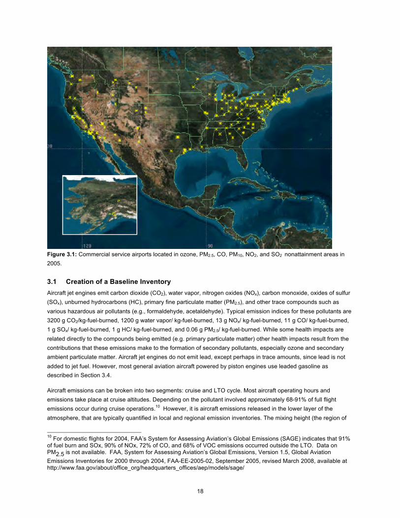
An assessment of the impact of aircraft emissions on air quality in NAAs was performed in this study. As is discussed further below, in 2005, there were a total of 118 NAAs in the US (see Table 3.1 below). Figure 3.1 shows the major commercial service airports located in ozone, PM2.5, CO, PM10, NO2, and SO2 NAAs.7 There were 150 airports located in these areas in 2005, of which 148 were included.8 This study also directly assessed the health impacts that result from the changes in air quality that could be attributable to aircraft operations. This section describes the three elements necessary to complete these study goals:

A baseline aircraft emissions inventory was developed to provide an estimate of criteria pollutants and precursor emissions attributable to aircraft operations from U.S. commercial service airports (Section 3.1);

Air quality modeling was performed to estimate the impacts of these emissions on ambient concentrations of PM and ozone9 (Section 3.2); and

Health impact analyses were conducted to determine the changes in public health endpoints if aircraft emissions at these airports were eliminated (Section 3.3).

In addition, an assessment of lead emissions from piston engine (general aviation) aircraft using aviation gasoline is provided (Section 3.4).

7 Airports were identified based on airports listed in the FAA’s Voluntary Airport Low Emissions Program (VALE), which focused on airports in CO, PM, and ozone non-attainment areas for 2005 see http://www.faa.gov/airports_airtraffic/airports/environmental/vale/media/vale_eligible_airports.xls. 8 148 of these airports were used in this study; Block Island State Airport (Block Island, Rhode Island) and Lake Hood Airport (Anchorage, Alaska) were not included due to insufficient aircraft operations data. 9 It is typical EPA practice to focus on PM and ozone impacts in air quality analyses due to their importance for human health. Note that ozone and PM2.5 nonattainment areas are more prevalent than NO2, SO2, CO, and lead nonattainment areas. Several EPA Regulatory Impact Analyses have considered changes in ambient concentrations of PM and ozone and resulting changes in health incidences (EPA 2005, EPA 2006).

18

Figure 3.1: Commercial service airports located in ozone, PM2.5, CO, PM10, NO2, and SO2 nonattainment areas in 2005.

3.1 Creation of a Baseline Inventory Aircraft jet engines emit carbon dioxide (CO2), water vapor, nitrogen oxides (NOx), carbon monoxide, oxides of sulfur (SOx), unburned hydrocarbons (HC), primary fine particulate matter (PM2.5), and other trace compounds such as various hazardous air pollutants (e.g., formaldehyde, acetaldehyde). Typical emission indices for these pollutants are 3200 g CO2/kg-fuel-burned, 1200 g water vapor/ kg-fuel-burned, 13 g NOx/ kg-fuel-burned, 11 g CO/ kg-fuel-burned, 1 g SOx/ kg-fuel-burned, 1 g HC/ kg-fuel-burned, and 0.06 g PM2.5/ kg-fuel-burned. While some health impacts are related directly to the compounds being emitted (e.g. primary particulate matter) other health impacts result from the contributions that these emissions make to the formation of secondary pollutants, especially ozone and secondary ambient particulate matter. Aircraft jet engines do not emit lead, except perhaps in trace amounts, since lead is not added to jet fuel. However, most general aviation aircraft powered by piston engines use leaded gasoline as described in Section 3.4.

Aircraft emissions can be broken into two segments: cruise and LTO cycle. Most aircraft operating hours and emissions take place at cruise altitudes. Depending on the pollutant involved approximately 68-91% of full flight emissions occur during cruise operations.10 However, it is aircraft emissions released in the lower layer of the atmosphere, that are typically quantified in local and regional emission inventories. The mixing height (the region of

10 For domestic flights for 2004, FAA’s System for Assessing Aviation’s Global Emissions (SAGE) indicates that 91% of fuel burn and SOx, 90% of NOx, 72% of CO, and 68% of VOC emissions occurred outside the LTO. Data on PM2.5 is not available. FAA, System for Assessing Aviation’s Global Emissions, Version 1.5, Global Aviation Emissions Inventories for 2000 through 2004, FAA-EE-2005-02, September 2005, revised March 2008, available at http://www.faa.gov/about/office_org/headquarters_offices/aep/models/sage/

19

the atmosphere near the earth’s surface in which turbulent mixing occurs) varies greatly by location, time of day, season, and synoptic meteorological pattern. For this study, we considered only emissions that occur below 3,000 feet above ground level; this is normally deemed equivalent to emissions which occur during the LTO cycle. The LTO cycle includes idle, taxi to and from terminal gates, take-off and climb-out, and approach to the airport. To provide an estimate of the contribution of aircraft to the total emissions inventories associated with non-natural sources, and to provide a basis for the air quality modeling, a baseline inventory of aircraft LTO cycle emissions was created as described below.

Airport Selection

An emissions inventory for the study was generated for 325 airports with commercial activity in the United States. Of these 325 airports, there are 263 commercial service airports and 62 airports that are either reliever or general aviation airports with commercial activity.11 The decision to include these 325 airports was made in two phases. First, the study participants estimated aircraft emissions from those commercial service airports located in the NAAs. The U.S. Federal Aviation Administration Voluntary Airport Low Emissions Program (VALE)12 identified 150 commercial service airports that are located in the 2005 ozone, PM2.5, CO, PM10, NO2, and SO2 NAAs areas as shown in Figure 3.1 and Table 3.1.

During the study, it also became apparent that aircraft emissions from upwind airports (in attainment areas) could influence air quality in NAAs because of atmospheric chemistry and regional transport processes. While it was not feasible to model aircraft emissions from all airports in the United States within the timeframe of this research, emissions data were generated for an additional 177 commercial service airports to account for upwind aircraft sources that could influence air quality in NAAs and to more fully estimate the impacts of aircraft activities. A total of 177 airports in attainment areas (those with the greatest number of operations and readily available flight operations data) were selected for inclusion in the analysis. The 325 airports modeled for the study cover all 50 states and approximately 95 percent of U.S. jet engine aircraft operations from June 2005 to May 2006 for which flight plans were filed (including commercial, military, and general aviation). (These airports also represent 95% of the operations with ICAO certified jet engines in the U.S.) The study includes 63 percent of all U.S. commercial service airports (325 of 515 airports). Figure 3.2 shows the 148 NAA airports and the additional 177 airports modeled for the study. A list of the 325 airports and their number of aircraft operations (and LTOs) is provided in Appendix B.

11 FAA’s National Plan of Integrated Airport Systems (NPIAS) report at http://www.faa.gov/airports_airtraffic/airports/planning_capacity/npias/reports/ . 12 http://www.faa.gov/airports_airtraffic/airports/environmental/vale/

20

Figure 3.2: 148 Nonattainment airports and the additional 177 modeled for the study

Data and Methods

The aircraft emissions inventory used for this study was created with the FAA Emissions and Dispersion Modeling System (EDMS), a computer program used to estimate emissions in and around airports, and to provide dispersion calculations around airports. EDMS was developed in the mid-1980’s (and has been regularly improved since that time) to assess the air quality impacts of proposed airport development projects. EDMS is the program required by the FAA for performing airport inventory and dispersion analyses for aviation.13

EDMS was used to generate an emissions inventory for LTO activity for flights arriving to, and departing from, the 325 study airports during the one-year period between June 2005 and May 2006. The inventory generated includes emissions from aircraft main engines, and also auxiliary power units (APUs). APUs are small, self-contained generators installed on aircraft that are used to start the main engines and to provide electricity and air conditioning to aircraft parked on the ground.

EDMS requires several data inputs. Operations data were obtained from the 2005 FAA Enhanced Traffic Management System (ETMS)14, the Bureau of Transportation Statistics (BTS) On Time Performance Data15, and the Air Traffic Activity Data System (ATADS).16 EDMS also requires jet fuel quality data, main engine and APU specifications, aircraft weight, and ground operating times. These data were obtained from a number of sources

13 More details regarding EDMS may be found at http://www.faa.gov/about/office_org/headquarters_offices/aep/models/edms_model/. 14 http://www.fly.faa.gov/Products/Information/ETMS/etms.html 15 http://www.transtats.bts.gov/OT_Delay/OT_DelayCause1.asp 16 http://aspm.faa.gov/main/atads.asp

21

including BTS17, the BACK fleet database18, and the National Airspace System Resources (NASR)19. Figure 3.3 shows the data inputs to EDMS.

Figure 3.3: Overview of EDMS inputs

EDMS computes emissions of primary particulate matter, CO, hydrocarbons,20 NOx, and SOx21

for all phases of taxi and flight based on ICAO engine emissions indices. Emissions indices are estimates of the mass of pollutant produced per mass of fuel consumed and are measured during engine certification testing and reported in the ICAO Engine Emissions Certification Databank.22 However, ICAO does not have a primary PM aircraft engine standard or test procedure, and, thus, PM emission indices are not reported in the ICAO Databank. To estimate total emissions of primary particulate matter (PM), a criteria pollutant composed of a complex mixture of solid particles and liquid droplets, EDMS relied on a research-based estimation technique to derive emissions indices from available data such as ICAO certification smoke number,23 and experimental results, as described more fully below.

Historically, primary PM emissions from aircraft have been difficult to estimate due to the lack of physical understanding of their formation and evolution in gas turbine engines and exhaust plumes, and the difficulty in measuring fine particles in the hot, high speed flow at the point where the exhaust exits the engine. Aircraft PM exhaust emission data are sparse, and test methods are still under development. ICAO and EPA do not have approved test methods or certification standards for aircraft PM emissions. ICAO’s Committee on Aviation 17 Bureau of Transportation Statistics, Airline On-Time Performance Data, June 2005 through May 2006, available from http://www.transtats.bts.gov/ 18 http://www.backaviation.com/Information_Services/ 19 Federal Aviation Administration, National Airspace System Resources (NASR) data, 2006. 20 Hydrocarbons are classified as non-methane hydrocarbons (NMHC) & volatile organic compounds (VOCs). VOCs play a role in the formation of ozone. 21 An error was made in the specification of the fuel sulfur level for some of the airports in this inventory such that the aircraft SO2 inventory is expected to be biased towards underestimating the contribution of aircraft by approximately a factor of 0.8. In particular, a fuel sulfur level of 400 ppm was assumed for some airports and 680 ppm was assumed for others. Our intention was to assume 680 ppm for all airports. However, variations of fuel sulfur of this level (±200ppm) are typical and are thus within the uncertainty of the estimation methods. 22 http://www.caa.co.uk/default.aspx?catid=702&pagetype=90 23 Smoke number is a dimensionless measure that quantifies smoke emissions from aircraft engines. ICAO requires smoke number testing for engine certification.

22

Environmental Protection (CAEP) has developed and approved the use of an interim First Order Approximation (FOA3)24 method to estimate total PM emissions (or total fine PM emissions) from certified aircraft engines. Subsequent to the completion of FOA3, the methodology was modified by adding margins to account for the potential effects of uncertainties that include the lack of a standard test procedure, poor definition of volatile PM formation in the aircraft plume, and the limited amount of data available on aircraft PM exhaust emission rates. This modified methodology is known as FOA3a. FOA3a is currently the agreed upon method to estimate PM emissions from aircraft engines, and it has been incorporated into the version of the FAA Emissions and Dispersion Modeling System (EDMS) that was used for this study, which was, version 5.02, June 2007. FOA3a predicts fine PM inventory levels that are approximately 5 times those predicted by FOA3 and reflects the scientific uncertainty associated with PM emissions rates from aircraft engines. This is discussed further in Appendix C.25

In addition to addressing the challenges of estimating aircraft PM emissions, another area requiring investigation was APU usage. APU usage depends on a range of factors including aircraft size, weather, and practices specific to individual airlines and pilots. One of the most important determinants of APU usage time is the availability of ground support equipment (e.g. preconditioned air) that can be used in place of the APU to heat or cool the cabin and provide ground-based power to aircraft parked at the gate. While many airlines have standard operating procedures for APU use, the ultimate decision rests with the pilot.

An APU usage survey was conducted and the results were integrated into EDMS for more accurate characterization of APU emissions. Because of the wide range of reported usage in the survey data, low, medium, and high values were analyzed to account for variations in aircraft size and the availability of ground support. For the study baseline inventory, a medium level of APU usage was used to account for a wide range of ground support access at the 325 airports, seasonal conditions, and other factors that define APU usage. The range of contribution of the medium level of APU usage to aircraft emissions below 3,000 feet is between 0% and slightly over 25%. The average is below 5% for CO and VOCs and under 10% for NOx and SOx. For only four non-attainment areas considered in this report, the medium level of APU usage contributes more than 1% to census area emissions (or total emissions) as estimated in the EPA year 2002 National Emissions Inventory. A description of the APU survey methods and results can be found in Appendix D.

24 Airport Air Quality Guidance Manual. Preliminary Edition 2007 (Doc 9889). http://www.icao.int/icaonet/dcs/9889/9889_en.pdf

23

Before discussing the inventory results, there is one other point which requires discussion. An error was made in the specification of the fuel sulfur level for 78 of the airports in this inventory such that the aircraft SO2 inventory is expected to be biased towards underestimating the contribution of aircraft by approximately a factor of 0.8. In particular, a fuel sulfur level of 400 ppm was assumed for some airports and 680 ppm was assumed for others. The intention was to use 680 ppm for all airports. However, variations of fuel sulfur of this level (±200 ppm) are typical and are thus within the uncertainty of the estimation methods.

Using the above data and methods, EDMS was used to generate an emissions inventory for each of the 325 study airports. A more detailed description of EDMS, baseline runs, data inputs, model specifications, limitations, and sources of discrepancies in the EDMS inventory are discussed in Appendix E.

Emissions Inventory Discussion

The first step in assessing the contribution of aircraft operations to NAAQS non-attainment is to develop emission inventories for the primary pollutants (NOx, SOx, HC, CO, and primary PM2.5) for each of the NAAs.26 There were a total of 118 NAAs identified for this study; each contained at least one commercial service airport. The NAAs in the study and the commercial service airports in each area are listed in Table 3.1 (see Appendix B for the airport name that coincides with the airport code), together with the pollutant(s) of concern. Of the 325 airports modeled, 148 commercial service airports were located in a NAA. Emissions from the remaining airports potentially contribute to the emission concentrations in these NAAs, due to atmospheric transport of emissions.

Table 3.1: List of nonattainment areas with at least one commercial service airport, as of September 7, 2005a

State EPA Green Book Nameb

Ozone (8-Hour)c,d,e CO PM10

PM2.5 (V=violation)

Notesf Airport Codeg

AK Anchorage, AK Serious ANC, MRI, LHD

AK Fairbanks, AK Serious FAI AL Jefferson Co, AL Subpart 1 V BHM AL Colbert Co, AL D MSL AZ Phoenix, AZ Subpart 1 Maintenance Serious PHX AZ Tucson, AZ Maintenance TUS AZ Mohave Co, AZ Maintenance IFP AZ Yuma, AZ Moderate YUM

26 Secondary pollutants such as ozone and secondary particulate matter are not emitted directly from aircraft engines and require air quality modeling to simulate their formation.

24



PM2.5 (V=violation)


CA Los Angeles South Coast Air Basin, CA Severe 17 Serious Serious V E

LAX, SNA, ONT, BUR, LGB

CA San Francisco-Oakland-San Jose, CA Marginal Maintenance SFO, OAK, SJC

CA San Diego, CA Subpart 1 SAN, CRQ

CA Sacramento Co, CA Serious Moderate SMF CA Coachella Valley, CA Serious Serious PSP

CA San Joaquin Valley, CA Serious Maintenance Serious V

FAT, BFL, MOD, SCK,

MCE, VIS CA San Bernardino Co, CA Moderate Moderate VCV CA Ventura Co, CA Moderate OXR CA Chico, CA Subpart 1 Maintenance CIC CA Indian Wells, CA Maintenance IYK CA Imperial Valley, CA Marginal Moderate IPL

CO Denver Metro, CO Subpt. 1 EACe Maintenance Maintenance DEN

CO Colorado Springs, CO Maintenance COS CO Aspen, CO Maintenance ASE CT Hartford-New Britain-Middletown, CT Moderate Maintenance BDL CT New Haven Co, CT Moderate Maintenance Moderate V HVN CT Greater Connecticut, CT Moderate GON GA Atlanta, GA Marginal V ATL

25



PM2.5 (V=violation)


GA Macon, GA Subpart 1 V MCN ID Boise-Northern Ada Co. ID Maintenance Maintenance BOI ID Fort Hall Reservation, ID Moderate PIH

IL Chicago-Gary-Lake Counties IL-IN Moderate V ORD, MDW, BLV

IN Marion County, IN Subpart 1 V IND IN Evansville, IN Subpart 1 V EVV KY Cinc.-Hamilton, OH-KY-IN Subpart 1 V CVG KY Louisville, KY-IN Subpart 1 V SDF MA Boston, MA Moderate Maintenance BOS MD Baltimore, MD Moderate V BWI MD Washington Co (Hagerstown), MD Subpart 1 EAC V HGR ME Portland, ME Marginal PWM ME Presque Isle, ME Maintenance PQI

ME Hancock, Knox, Lincoln & Waldo Counties, ME

Subpart 1 RKD, BHB

MI Detroit-Ann Arbor, MI Marginal V DTW MI Grand Rapids, MI Subpart 1 GRR MI Flint, MI Subpart 1 FNT MI Lansing-East Lansing, MI Subpart 1 LAN MI Kalam.-Battle Creek, MI Subpart 1 AZO MI Muskegon, MI Marginal MKG MN Minneapolis-St Paul, MN Maintenance C MSP MN Duluth, MN Maintenance DLH MO St Louis, MO Moderate Maintenance V STL MT Laurel Area,Yellowstone Co. Maintenance BIL

MT East Helena Area (Lewis and Clark Co.), MT

B,D HLN

26



PM2.5 (V=violation)


MT Butte, MT Moderate BTM NC Charlotte, NC Moderate Maintenance CLT NC Raleigh-Durham, NC Subpart 1 Maintenance RDU

NC Greensboro-Winston Salem-High Point, NC

Moderate EACe V GSO

NC Fayetteville, NC Subpart 1 EAC FAY

NH Boston-Lawrence-Worcester (E. MA), MA Moderate Maintenance MHT

NH Portsmouth-Dover-Rochester,NH Moderate PSM

NJ New York-N. New Jersey-Long Island, NY-NJ-CT

Moderate Maintenance V

EWR, JFK, LGA,

ISP, HPN NJ Atlantic City, NJ Moderate Maintenance ACY NJ Trenton, NJ Moderate Maintenance V TTN NM Albuquerque, NM Maintenance ABQ

NV Clark Co, NV Subpart 1 Maintenance Serious LAS, VGT, HND

NV Washoe Co, NV Moderate <= 12.7ppm

Serious RNO

NY Buffalo-Niagara Falls, NY Subpart 1 BUF

NY Albany-Schenectady-Troy, NY Subpart 1 ALB

NY Rochester, NY Subpart 1 ROC NY Syracuse, NY Maintenance SYR NY Poughkeepsie, NY Moderate V SWF NY Jamestown, NY Subpart 1 JHW OH Cuyahoga Co, OH Moderate Maintenance Maintenance V C CLE

27



PM2.5 (V=violation)


OH Columbus, OH Subpart 1 V CMH, LCK

OH Dayton-Springfield, OH Subpart 1 V DAY OH Cleve.-Akron-Lorain,OH Moderate V CAK OH Lucas Co, OH Subpart 1 TOL OH Youn.-Warren-Shar.OH-PA Subpart 1 YNG OR Portland OR-Vancouver WA area Maintenance PDX OR Medford-Ashland, OR Maintenance Moderate MFR OR Klamath Falls, OR Maintenance Maintenance LMT PA Phil.-Wilmington-Atl. City, PA-NJ-MD-DE Moderate V PHL PA Hazelwood, PA Subpart 1 Maintenance V PIT PA Harris.-Lebanon-Carlisle,PA Subpart 1 V MDT PA Allen.-Bethl.-Easton, PA Subpart 1 ABE PA Scranton-Wilkes-Barre, PA Subpart 1 AVP PA Erie, PA Subpart 1 ERI PA State College, PA Subpart 1 UNV PA Reading, PA Subpart 1 V RDG PA Pitts.-Beaver Valley, PA Subpart 1 V LBE PA Johnstown, PA Subpart 1 V JST PA Altoona, PA Subpart 1 AOO

RI Providence (All RI), RI Moderate PVD, WST, BID

SC Greenville-Spartanburg-Anderson, SC Subpart 1 EAC V GSP SC Columbia, SC Subpart 1 EAC CAE TN Memphis, TN Marginal Maintenance MEM

TN Nashville, TN Subpt. 1 EACe BNA

TN Knoxville, TN Subpart 1 V TYS TN Chattanooga, TN-GA Subpart 1 EAC V CHA

28



PM2.5 (V=violation)


TN Johnson City-Kingsport-Bristol, TN Subpart 1 EAC TRI

TX Dallas-Fort Worth, TX Moderate DFW, DAL

TX Houston-Galvest.-Braz, TX Moderate

IAH, HOU, EFD, LBX

TX San Antonio, TX Subpart 1 EAC SAT TX El Paso Co, TX Moderate ELP TX Beaumont-Port Arthur, TX Marginal BPT UT Salt Lake Co, UT Maintenance Moderate C SLC VA Washington, DC-MD-VA Moderate Maintenance V IAD, DCA

VA Norfolk-Virginia Beach-Newport News (HR),VA

Marginal ORF, PHF

VA Richmond-Petersburg, VA Marginal RIC VA Roanoke, VA Subpart 1 EAC ROA

WA Seattle-Tacoma, WA Maintenance SEA WA Spokane Co, WA Serious Moderate GEG WA Yakima Co, WA Moderate YKM WA King Co, WA Maintenance Maintenance BFI WI Milwaukee, WI Moderate C MKE WI Madison, WI C MSN WV Charleston, WV Subpart 1 V CRW WV Huntingt.-Ashland,WV-KY Subpart 1 V HTS WV Parkersb.-Marietta,WV-OH Subpart 1 V PKB WY Sheridan, WY Moderate SHR

Notes:

29



PM2.5 (V=violation)


a Commercial service airports listed in the National Plan for Integrated Airport Systems (NPIAS) per §47102(7) of Title 49 USC.

An empty cell in criteria pollutant columns indicates that the airport is in attainment for that pollutant.

b Green Book Name is the name of the nonattainment area.

c The 8-hr. ozone national ambient air quality standard took effect on June 15, 2005, replacing the previous 1-hr. standard.

d "Subpart 1" denotes 8-hour ozone nonattainment areas that are covered under Subpart 1, Part D, Title I of the Clean Air Act. "Subpart 1" is considered nonattainment without a classification.

e Early Action Compacts (EACs) are not a classification, but areas for which the effective date of their nonattainment designation has been deferred because they are expected to reach or maintain attainment status by December 31, 2006.

f Notes description below:

A - Lead nonattainment or maintenance confirmed

D - SO2 nonattainment or maintenance unconfirmed

B - Lead nonattainment or maintenance not confirmed

E - NO2 nonattainment or maintenance confirmed

C - SO2 nonattainment or maintenance confirmed

F - NO2 nonattainment or maintenance unconfirmed

g The two airports that were not included in the study because of insufficient operations data are Block Island State Airport (BID) and Lake Hood Airport (LHD).

BID is in Block Island, Rhode Island and LHD is Anchorage, Alaska.

30

As part of this process, a quantitative comparison of the baseline aircraft inventory to total county level emissions inventories was performed for the primary pollutants. The county level inventories used for the aircraft inventory comparison shown in this section were derived from EPA’s year 2002 National Emissions Inventory (NEI), a database of criteria pollutants and their precursors. The NEI provides emissions by Federal Information Processing Standards (FIPS) area; FIPS are generally the same as counties. An estimate of all FIPS area emissions was obtained by aggregating NEI data from all sources including point sources (e.g. smokestacks at a factory), mobile sources (e.g. cars) and area sources (e.g. gas stations). While the NEI does include aircraft emissions, the baseline aircraft emission inventory for each airport in this study was based on EDMS as described above, rather than the NEI. 27 That is, the baseline aircraft emissions inventory for each airport for the period June 2005 through May 2006 were used and aircraft emissions originally within the NEI were removed. The NAA and regional inventories were built from this county level inventory information. As presented below, the aircraft emissions inventory was then compared with total emissions inventories (which thus included EDMS aircraft emissions rather than NEI aircraft emissions) to get a measure of relative contributions.

Focusing first on the NAAs, Table 3.2, below, shows a distribution of the percent contribution of emissions for aircraft in the 118 NAAs. The average value in each row reflects the average of the values for aircraft contributions in each of the 118 NAAs. 28 As seen in Table 3.2 the aircraft LTO emissions at the 148 commercial service airports within the 118 NAAs are small. (Note, some of the general aviation airports and reliever airports studied were located in NAAs, but they were not included with the below inventories for NAAs. The aircraft emissions from these airports are estimated to be a small fraction of the aircraft emissions in NAAs compared to those from commercial service airports. This is because commercial aircraft are generally larger than general aviation aircraft and thus burn more fuel; emissions are proportional to fuel burn.)

Table 3.2: Contribution of U.S. aircraft LTO operations at 148 commercial service airports to emission inventories in 118 NAAs a, b, c, d

Aircraft Emissions Inventory CO NOx VOCs SOx PM2.5

2002: Average and range as a percentage of aircraft LTO contributions to emission inventories for 118 NAA with at least one commercial service airport

0.44%

0.06% to 4.36%

0.66%

0.004% to 10.93%

0.48%

0.05% to 5.03%

0.37%

0.002% to 6.91%

0.15%

0.002% to 2.57%

Notes: a This table presents aircraft LTO emission inventories for the 148 commercial service airports in the nonattainment

27 EDMS aircraft emissions were used instead of NEI aircraft emissions because the level of fidelity for modeling aircraft in the 2001 NEI is lower than that for the inventories used for this study. In particular, NEI emissions for commercial aircraft were generated using the default EDMS times in mode (0.7 minutes for take-off, 2.2 minutes for climb-out, 4 minutes for approach, and 26 minutes for taxi and ground idle). Also, aircraft PM emissions in the 2001 NEI were based on several engines with PM emissions data in AP 42, which is an EPA publication of air pollutant emissions factors (http://www.epa.gov/ttn/chief/ap42/). For the aircraft inventory comparison in this study, NEI commercial aircraft emissions were instead replaced with aircraft emissions generated for this study using a newer version of EDMS (version 5.02) along with actual aircraft operational data and the PM emissions estimation method FOA3a as described in Appendix E. See Appendix J for a comparison of EDMS aircraft emissions with the 2002 NEI. 28 If the values were calculated as total aircraft emissions over total NAA area inventories for each pollutant the values for each pollutant for 2002/2020 would be as follows: CO: 0.36/0.78%, NOx: 0.80/2.27%, VOCs: 0.43/0.77%, SOx: 0.12/0.32%, PM2.5: 0.16/0.24%.

31

areas. b If an area had more than type of nonattainment area (e.g., PM2.5 and CO nonattainment areas), the nonattainment area was selected based on the area with the largest population base. c Except for aircraft, the emission levels for categories are from the inventories developed for the 2008 Final Rule on Emission Standards for New Nonroad Spark-Ignition Engines, Equipment, and Vessels, which is available at http://www.epa.gov/otaq/equip-ld.htm . d 2005 is the base year for aircraft emissions.

Looking deeper into the information, Table 3.3 and Table 3.4 show the top 25 PM2.5 and NOx aircraft emission inventory NAAs ranked according to the percent of inventory contributed by aircraft emissions (from commercial service airports). Table 3.3 shows that for PM2.5, 9 of the areas with the greatest aircraft direct PM contributions were also PM2.5 NAAs in 2005. Similarly for ozone, Table 3.4 shows that 16 of the areas with the greatest aircraft NOx contributions were ozone NAAs in 2005 (as described earlier, 2002 is the base year for non-aircraft emissions, and 2005 is the base year for aircraft emissions).

Table 3.3: Top 25 NAAs according to aircraft PM2.5 contribution

NAA Name % of total % of

mobile Anchorage 2.57% 8.88% Memphis 1.14% 4.06% Salt Lake City 0.85% 3.99% Las Vegas 0.68% 3.20% Aspen 0.44% 5.20% New York-N. New Jersey-Long Island* 0.41% 1.48% Louisville* 0.39% 2.90% Minneapolis-St. Paul 0.39% 1.87% Chicago-Gary-Lake County* 0.36% 1.37% Providence (all of RI) 0.31% 1.06% Denver-Boulder-Greeley-Ft. Collins-Love. Area 0.31% 1.65% Phoenix-Mesa 0.30% 1.29% San Francisco-Bay Area 0.29% 1.23% Charlotte-Gastonia-Rock Hill 0.29% 1.56% Los Angeles-South Coast Air Basin* 0.27% 0.92% Southeast Desert Modified AQMA (Riverside County, CA - Coachella Valley, CA Area)

0.27% 0.98%

Cincinnati-Hamilton* 0.26% 2.27% Detroit-Ann Arbor* 0.26% 1.27% Seattle-Tacoma 0.25% 0.87% Dallas-Fort Worth 0.23% 1.52% Atlanta* 0.23% 1.74% Syracuse 0.22% 1.10% Washington DC* 0.21% 1.49% Philadelphia-Wilmington-Trenton* 0.20% 0.85%

32

NAA Name % of total % of

mobile Albuquerque 0.19% 1.28%

* 2005 PM2.5 NAA according to Table 3.1.

Table 3.4: Top 25 NAAs according to aircraft NOx contribution

NAA name % of total % of

mobile Anchorage 10.93% 19.63% Aspen 4.45% 5.16% Memphis* 3.23% 4.76% Las Vegas* 3.06% 7.13% Salt Lake City 2.98% 3.64% Dallas-Fort Worth* 1.76% 2.27% Reno 1.73% 2.07% Phoenix-Mesa* 1.72% 1.87% San Francisco-Bay Area* 1.57% 1.85% Lake Tahoe Nevada (Washoe County) 1.43% 1.75% Denver-Boulder-Greeley-Ft. Collins-Love. Area* 1.42% 2.13% New York-N. New Jersey-Long Island* 1.40% 1.98% Charlotte-Gastonia-Rock Hill* 1.39% 2.05% Atlanta* 1.32% 2.19% Albuquerque 1.27% 1.62% Chicago-Gary-Lake County* 1.27% 1.93% Washington DC* 1.22% 1.93% Minneapolis-St. Paul 1.07% 1.90% Southeast Desert Modified AQMA (Riverside County, CA - Coachella Valley, CA Area)*

1.07% 1.28%

Seattle-Tacoma 1.03% 1.15% Indianapolis* 1.02% 1.42% Los Angeles-South Coast Air Basin* 1.02% 1.21% San Diego* 0.99% 1.07% Providence (all of RI)* 0.95% 1.19% El Paso 0.84% 1.11%

*2005 Ozone NAA according to Table 3.1.

33

It is also interesting to consider these inventory contributions from other perspectives. For the 118 NAAs listed in Table 3.1, Table 3.5 shows the 25 which are the busiest based on the total number of LTOs at all commercial service airports in that NAA. Of these, 21 of 25 were either an ozone or PM2.5 NAA, or both, in 2005 (10 areas both ozone and PM2.5 NAAs, 21 ozone NAAs, and 10 PM2.5 NAAs). The airports associated with these LTOs are among the busiest in the nation. Also for the 118 NAAs listed above, Table 3.6 shows the 25 largest NAAs by population. The population (based on population data for the year 2000) in these NAAs represents 74 percent of those in all 118 NAAs. Many of the same busy airports are also shown in Table 3.5. Of the 25 large population centers in Table 3.6, 24 were either an ozone or PM 2.5 NAA, or both in 2005 (14 areas both ozone and PM2.5 NAAs, 24 ozone NAAs, and 14 PM2.5 NAAs). Both of these analyses indicate that airports are an important emissions source in these NAAs.

Table 3.5: Aircraft emissions contribution for top 25 NAAs according to LTOs (NOx, VOCs, and PM2.5)

NOx VOCs PM2.5 NAA Name 2005 LTOs % total % mobile % total % mobile % total % mobile

Los Angeles-South Coast Air Basina,b 937,157 1.02% 1.21% 0.50% 0.97% 0.27% 0.92% New York-N. New Jersey-Long Islanda,b

930,014 1.40% 1.98% 0.42% 0.93% 0.41% 1.48%

Southeast Desert Modified AQMA (Riverside County, CA - Coachella Valley, CA Area) a

756,196 1.07% 1.28% 0.54% 1.04% 0.27% 0.98%

Chicago-Gary-Lake Countya,b 660,721 1.27% 1.93% 0.49% 1.02% 0.36% 1.37% Houston-Galveston-Brazoriaa 512,986 0.68% 1.08% 0.49% 1.25% 0.16% 0.81% Atlantaa,b 491,426 1.32% 2.19% 0.54% 1.10% 0.23% 1.74% Dallas-Fort Wortha 486,402 1.76% 2.27% 0.58% 1.05% 0.23% 1.52% Las Vegasa 481,057 3.06% 7.13% 1.71% 2.34% 0.68% 3.20% San Francisco-Bay Areaa 469,251 1.57% 1.85% 0.63% 1.20% 0.29% 1.23% Washington DCa,b 393,169 1.22% 1.93% 0.57% 1.14% 0.21% 1.49% Philadelphia-Wilmington-Trentona,b 380,249 0.64% 0.92% 0.35% 0.74% 0.20% 0.85% Seattle-Tacoma 318,786 1.03% 1.15% 0.28% 0.45% 0.25% 0.87% Phoenix-Mesaa 308,259 1.72% 1.87% 0.61% 1.12% 0.30% 1.29% Denver-Boulder-Greeley-Ft. Collins-Lovea

303,065 1.42% 0.67% 0.54% 0.58% 0.31% 0.60%

Boston-Worcester-Manchestera 282,139 0.78% 1.17% 0.35% 0.87% 0.11% 0.93% Charlotte-Gastonia-Rock Hilla 265,175 1.39% 2.05% 0.69% 1.70% 0.29% 1.56%

34

NOx VOCs PM2.5 NAA Name 2005 LTOs % total % mobile % total % mobile % total % mobile

Detroit-Ann Arbora,b 255,504 0.64% 1.06% 0.42% 0.73% 0.26% 1.27% Minneapolis-St. Paul 254,326 1.07% 1.90% 0.59% 1.05% 0.39% 1.87% San Joaquin Valleya,b 249,458 0.04% 0.06% 0.10% 0.29% 0.01% 0.06% Anchorage 248,459 10.93% 19.63% 3.89% 5.78% 2.57% 8.88% Salt Lake City 227,358 2.98% 3.64% 1.13% 2.12% 0.85% 3.99% San Diegoa 222,798 0.99% 1.07% 0.37% 0.76% 0.16% 0.63% Cincinnati-Hamiltona,b 220,115 0.62% 1.37% 1.45% 2.99% 0.26% 2.27% Memphisa 196,202 3.23% 4.76% 2.95% 5.93% 1.14% 4.06% Cleveland-Akron-Loraina,b 184,501 0.41% 0.62% 0.33% 0.62% 0.13% 0.51%

Notes: a Ozone NAA in 2005 according to Table 3.1. b PM2.5 NAA in 2005 according to Table 3.1.

Table 3.6: Aircraft emissions contribution for top 25 NAAs according to population (NOx, VOCs, and PM2.5)

NOx VOCs PM2.5 NAA Name

Year 2000 Population % total % mobile % total % mobile % total % mobile

New York-N. New Jersey-Long Islanda,b

20,364,647 1.40% 1.98% 0.42% 0.93% 0.41% 1.48%

Los Angeles-South Coast Air Basina,b

14,593,587 1.02% 1.21% 0.50% 0.97% 0.27% 0.92%

Chicago-Gary-Lake Countya,b 8,757,808 1.27% 1.93% 0.49% 1.02% 0.36% 1.37% Philadelphia-Wilmington-Trentona,b

7,333,475 0.64% 0.92% 0.35% 0.74% 0.20% 0.85%

San Francisco-Bay Areaa 6,576,113 1.57% 1.85% 0.63% 1.20% 0.29% 1.23%

Boston-Worcester-Manchestera 6,230,843 0.78% 1.17% 0.35% 0.87% 0.11% 0.93% Dallas-Fort Wortha 5,030,828 1.76% 2.27% 0.58% 1.05% 0.23% 1.52%

Detroit-Ann Arbora,b 4,932,383 0.64% 1.06% 0.42% 0.73% 0.26% 1.27%

Houston-Galveston-Brazoriaa 4,669,571 0.68% 1.08% 0.49% 1.25% 0.16% 0.81%

Washington DCa,b 4,654,618 1.22% 1.93% 0.57% 1.14% 0.21% 1.49%

35

NOx VOCs PM2.5 NAA Name

Year 2000 Population % total % mobile % total % mobile % total % mobile

Atlantaa,b 4,231,750 1.32% 2.19% 0.54% 1.10% 0.23% 1.74%

San Joaquin Valleya,b 3,290,618 0.04% 0.06% 0.10% 0.29% 0.01% 0.06%

Phoenix-Mesaa 3,111,876 1.72% 1.87% 0.61% 1.12% 0.30% 1.29%

Cleveland-Akron-Loraina,b 2,945,575 0.41% 0.62% 0.33% 0.62% 0.13% 0.51%

San Diegoa 2,813,431 0.99% 1.07% 0.37% 0.76% 0.16% 0.63%

Minneapolis-St. Paul 2,723,925 1.07% 1.90% 0.59% 1.05% 0.39% 1.87% Denver-Boulder-Greeley-Ft. Collins-Loveland Areaa,

2,715,806 1.42% 2.13% 0.54% 1.42% 0.31% 1.65%

Baltimorea 2,512,431 0.82% 1.40% 0.30% 0.70% 0.14% 1.04% Greater Connecticut (Hartford-New Britain-Middletown Area, New Haven County)a,b

2,510,470 0.41% 0.52% 0.12% 0.28% 0.08% 0.41%

St. Louisa,b 2,508,230 0.34% 0.58% 0.26% 0.57% 0.08% 0.48%

Pittsburgh-Beaver Valleya,b 2,433,999 0.26% 0.62% 0.39% 0.80% 0.05% 0.63%

Sacramento Metroa 1,978,348 0.61% 0.74% 0.28% 0.54% 0.07% 0.53%

Cincinnati-Hamiltona,b 1,891,518 0.62% 1.37% 1.45% 2.99% 0.26% 2.27%

Milwaukee-Racinea 1,839,149 0.45% 0.81% 0.33% 0.99% 0.12% 0.82%

Indianapolisa,b 1,607,486 1.02% 1.42% 0.63% 1.17% 0.13% 1.02%

Notes: a Ozone NAA in 2005 according to Table 3.1. b PM2.5 NAA in 2005 according to Table 3.1.

It is also interesting to consider aircraft emissions in the context of other mobile source emission categories for the 118 NAAs. For example, Table 3.7 and Table 3.8 present NOx and PM2.5 emissions for mobile source categories, including aircraft at the 148 commercial service airports. 2002 is the base year for non-aircraft emissions and 2005 is the base year for aircraft emissions. Appendix J contains similar information for VOCs, CO, and SOx.

36

Table 3.7: Nonattainment area annual NOx emission levels for mobile sources(metric tons)a,b,c,d

Source NOx Aircraft 73,152 Recreational Marine Diesel

13,520


398,338


755,208


105,414

Small Nonroad SI 83,735 Recreational Marine SI 27,661 SI Recreational Vehicles

2,411


168,424

Locomotive 330,894 Total Off-Highway 1,958,755 Highway non-diesel 2,229,330 Highway Diesel 1,683,882 Total Highway 3,913,213 Total Mobile Sources 5,871,967

Notes: a This table presents aircraft LTO emission inventories for the 148 commercial service airports in the nonattainment areas. b If an area had more than type of nonattainment area (e.g., PM2.5 and CO nonattainment areas), the nonattainment area was selected based on the area with the largest population base. c Except for aircraft, the emission levels for categories are from the inventories developed for the 2008 Final Rule on Emission Standards for New Nonroad Spark-Ignition Engines, Equipment, and Vessels, which is available at http://www.epa.gov/otaq/equip-ld.htm . d 2005 is the base year for aircraft emissions.

Table 3.8: Nonattainment area annual PM2.5 emission levels for mobile sources (metric tons)a,b,c,d

Source PM2.5

Aircraft 1,948 Recreational Marine Diesel

368


14,342


65,572


5,475

37

Source PM2.5

Small Nonroad SI 14,304 Recreational Marine SI

6,488


2,668


833

Locomotive 8,301 Total Off-Highway 120,299 Highway non-diesel 28,504 Highway Diesel 42,729 Total Highway 71,233 Total Mobile Sources

191,532


As is shown in Table 3.2 above and also included in Table 3.9, aircraft operations at the 148 commercial service airports in the 118 NAAs are a relatively small source of emissions in these areas. Finally, as presented in Table 3.9, the study also examined contributions to national inventories for both mobile sources and total emissions for the 325 commercial service airports.

Table 3.9: Contribution of aircraft LTO operations at commercial service airports to emissions inventories

Aircraft emissions inventory CO NOx VOCs SOx PM2.5 2002: average and range as a percentage of total emissions inventories in 118 NAAs with at least one commercial service airport (118 airports)

0.44%

0.06% to 4.36%

0.66%

0.004% to 10.93%

0.48%

0.05% to 5.03%

0.37%

0.002% to 6.91%

0.15%

0.002-2.57%

2002: average and range as a percentage of Mobile Source emissions inventories in 118 NAAs with at least one commercial service airport (118 airports)

0.54%

0.089% to 4.72%

1.04%

0.014% to 19.63%

0.98%

0.064%% to 9.04%

2.24%

0.026% to 30.92%

0.84%

0.016% to 8.88%

38

Aircraft emissions inventory CO NOx VOCs SOx PM2.5 As a percentage of EPA year 2002 National Emissions Inventory (325 airports)

0.18% 0.41% 0.23% 0.07% 0.05%

As a percentage of Mobile Source emissions inventory in EPA year 2002 National Emissions Inventory (325 airports)

0.22% 0.71% 0.51% 1.29% 0.53%

39

3.2 Impact of Aircraft Emissions on Ambient Air Quality The results of the baseline emissions inventory comparison presented in the previous section offer a first estimate of aviation’s influence on air quality. However, these primary pollutants are subject to atmospheric transport and atmospheric chemistry processes that affect air quality levels downwind of primary sources. Atmospheric residence times can extend for multiple days and it is important to consider regional scales even when assessing aircraft emissions from distinct airport locations. Further, these processes lead to the formation of secondary pollutants such as ozone and secondary particulate matter – the latter results from the condensation of chemical species minutes to days after emission of the precursor emissions (predominantly NOx and SOx for aircraft). To determine the impact of the baseline aircraft emissions inventory on air quality, a national-scale air quality simulation was performed for the study.

Air Quality Modeling Simulation- Data and Methods

Consistent with EPA analyses such as the Clean Air Interstate Rule Regulatory Impact Analysis (EPA 2005), the air quality modeling performed for the study included the formation, transport, and destruction of two pollutants: ozone and fine particulate matter (PM2.5). These two pollutants are expected to be the dominant causes of human health impacts associated with local air quality. To model changes in 8-hour ozone29 and annual average PM2.5

30 concentrations, an air quality simulation was performed using the Community Multiscale Air Quality (CMAQ) modeling system, a three dimensional grid-based, air quality model designed to estimate the fate of ozone precursors and primary and secondary particulate matter concentrations and their deposition over regional and urban scales (Byun and Schere 2006). The analysis used a 36 km x 36 km grid scale that is expected to lead to an underestimation of some local effects close to airport boundaries.

Inputs to the CMAQ modeling system include emissions estimates (from aircraft and other sources), initial/boundary conditions, and meteorological fields. While the baseline emissions inventory from EDMS for June 2005 through May 2006 was used to estimate total emissions from aircraft (see section 3.1), emissions estimates for non-aircraft sources were obtained from the EPA year 2001 National Emissions Inventory (NEI). The 2001 NEI, rather than the 2002 NEI, was used for the modeling of aircraft emissions impacts on air quality and human health because it was the most carefully assessed national inventory at the time and it was readily available for air quality modeling -- it had already been used for other rulemakings such as the proposed rule for "Control of Emissions of Air Pollution from Locomotives and Marine Compression-Ignition Engines Less than 30 Liters per Cylinder", 72 FR 15938, April 3, 2007. For the annual PM2.5 estimates, an entire year of meteorology was modeled. For 8-hour ozone estimates, a five month simulation was performed to account for the summer months in which ozone concentrations peak (May through September).

The air quality modeling methods used in this study have been used to support several regulatory actions initiated by EPA, including the final PM2.5 NAAQS (EPA 2006), the 8-hour Ozone NAAQS (EPA 2008), and the rule for the "Control of Emissions of Air Pollution from Locomotives and Marine Compression-Ignition Engines Less than 30 Liters per Cylinder" (EPA 2007c). A detailed description of the air quality modeling methods used for the study can be found in Appendix F.

Air Quality Modeling Results

For the study, three national emission scenarios were modeled with CMAQ to estimate the potential air quality impacts of aircraft emissions: a base line scenario with all 2001 NEI emissions (including NEI aircraft emissions), an 29 Given in parts per billion (ppb). The averaging time for the ozone NAAQS is 8 hours. 30 Given in micrograms per cubic meter (µg/m3). The PM NAAQS is expressed as an annual average. There is also a 24-hour PM2.5 NAAQS; however, this study only considered the annual average.

40

EDMS aircraft emissions scenario with a full set of emissions data for non-aircraft sources obtained from the 2001 NEI plus the specific aircraft emissions generated in the EDMS baseline inventory (see Section 3.1), and another with all aircraft emissions (both EDMS and NEI) removed. The difference in estimated pollutant concentrations between these two simulations was used to determine the local and regional air quality impacts of the aircraft emissions. The approach used is consistent with the EPA guidance document for modeling ozone and PM2.5 (EPA 2007b) and is described more fully in Appendix F.

Turning first to PM2.5, almost all areas experienced increases in annual average PM2.5 concentrations due to modeled aircraft emissions. The CMAQ simulation for PM2.5 utilized data from 557 counties with monitoring systems for this emission. Of the 557 counties with PM2.5 monitoring data, 546 showed increases, 9 showed no change, and 2 showed decreases of less than 0.001 µg/m3; these decreases are expected to be within the range of model uncertainty. On average, the modeling revealed that aircraft emissions contribute 0.01 µg/m3 to overall annual average ambient PM2.5 levels.

The largest impact was found in Riverside County, CA where modeled aircraft emissions increased annual average PM2.5 values by 0.15 µg/m3 (a 0.52% increase from 28.73 to 28.88 µg/m3).

San Bernardino County, CA also showed an impact greater than 0.10 µg/m3. Another 13 counties showed an impact of at least 0.05 µg/m3 and another 38 counties in the U.S. had an impact of at least 0.02 µg/m3.

The results of the PM modeling for NAAs and all counties appear below in Table 3.10. Figure 3.4 shows a map of the national changes in average annual PM determined by the air quality simulation. The individual results for the 557 U.S. counties with PM2.5 monitoring data are provided in Appendix F.

Table 3.10: Average annual PM2.5 estimates. Results are given in µg/m3. The annual National Ambient Air Quality Standard for PM2.5 is 15.0 µg/m3.

Without Aircraft

Emissions (µg/m3)

With Aircraft Emissions

(µg/m3)

Percent Increase Due

to Aircraft Emissions

Non-Attainment Areas

17.75 17.76 0.06%

All Counties 12.59 12.60 0.08%

41

Figure 3.4: Estimated change in annual PM2.5 concentrations (µg/m3) due to aircraft emissions.

For ozone, the analysis revealed a mix of potential benefits and disbenefits resulting from aircraft emissions. The photochemistry associated with ozone formation is complex, depending on local quantities of NOx, VOCs, and other ozone catalysts. Normally, increasing NOx emissions increases ozone concentrations in suburban and rural areas where VOC sources are plentiful. Sometimes however, the addition of NOx emissions (from aircraft and other sources) decreases ozone concentrations in urban cores, where VOC concentrations are more limited. The air quality modeling simulation revealed areas in which the addition of aircraft emissions increased ozone as well as areas in which decreased ozone concentrations (sometimes referred to as ozone or NOx disbenefits) were projected:

The CMAQ simulation for ozone utilized monitoring data from 571 U.S. counties. For all of these counties, the average change in 8-hour average ozone values was found to be an increase of 0.10 parts per billion (ppb) due to modeled aircraft emissions. The largest increase due to aircraft emissions occurred near the Atlanta area, a 0.6% increase from 95.9 to 96.5 ppb.

However, there were 24 counties across the U.S. where modeled aircraft emissions caused a decrease in 8-hour ozone values. The largest reduction was projected in Richmond County, NY, a 0.3% decrease from 96.3 to 96.0 ppb.

A summary of the results of the ozone modeling for NAAs and all counties appears below in Table 3.11. Individual results for the 571 U.S. counties with valid ozone monitoring data are provided in Appendix F. Figure 3.5 depicts the

42

county-level changes in 8-hour ozone determined by the air quality simulation.

Table 3.11: Average 8-hour ozone values (ppb) with and without EDMS aircraft emissions. The National Ambient Air Quality Standard for 8 hour ozone is 80 ppb. Based on rounding convention, values greater than or equal to 85 ppb are considered non-attainment.

Without Aircraft

Emissions (ppb)

With Aircraft Emissions (ppb)

Percent Increase Due to

Aircraft Emissions Nonattainment Areas 91.10 91.21 0.12%

All Counties 84.85 84.95 0.12%

Figure 3.5: Estimated change in 8-hour ozone concentrations (ppb) due to aircraft emissions. Negative values represent regions where aircraft emissions reduce levels of ozone. Positive values represent regions where the aircraft emissions increase ozone levels.

The air quality modeling results presented above depict changes in ambient concentrations of ozone and PM that influence attainment of National Ambient Air Quality Standards and may result in changes in public health.31 The 31 Note that on March 27 of 2008, EPA published a rule revising the primary ozone NAAQS from 0.08 ppm to 0.075 ppm and setting the secondary ozone NAAQS to 0.075 ppm, effective May 27 of 2008. 73 FR 16436. Nonattainment statuses of the counties assessed in this study are from 2005; the effect of the new ozone NAAQS on the nonattainment statuses of these counties was not considered in this study.

43

following section describes the health impact analysis that was performed to assess the changes in public health due to aircraft contributions to ozone and ambient fine PM concentrations.

3.3 The Impact of Aircraft Emissions on Public Health The health impact analysis performed for this study used a methodology consistent with benefit analyses performed by EPA for the PM NAAQS and the Ozone NAAQS (EPA 2006; EPA 2008). It should be noted that there are data limitations and uncertainties that may affect the results by an unknown amount (in terms of both under- and over-estimates). The use of a 36 km x 36 km grid cell size for the air quality analyses is expected to underestimate health impacts, especially those that may occur close to airport boundaries. The omission of air quality impacts from airports not included in this analysis is expected to lead to underestimation of aircraft-related health impacts. Omitting the effect of cruise level emissions on surface air quality is also expected to lead to underestimation of health impacts by an unknown amount. Further, analysis of only one year may lead to overestimation or underestimation of aircraft impacts due to year-to-year changes in meteorology. Non-aircraft sources were also not included (e.g. emissions of ground service equipment and other aircraft sources). Finally, we report the results for one concentration-response relationship for the health effects of ambient PM; a range of concentration-response relationships has been reported in the literature. The net effect of these assumptions and limitations is not known. Further research is recommended into these areas.32

EPA’s general health impact analysis framework uses the following framework (EPA 2006):

Given baseline and post-control33 emissions inventories, EPA uses photochemical air quality modeling to estimate baseline and post-control ambient concentrations of the pollutant of concern.

Changes in ambient concentrations of that pollutant are then combined with monitoring data to estimate population-level potential exposure to changes in ambient concentrations.

Changes in population exposure are then used as input to impact functions to generate changes in the incidences of health effects, or changes in other exposure metrics are input into dose-response functions to generate changes in welfare effects.

The results of the air quality modeling described in the previous section were used as inputs to determine changes in human health effects across the continental United States. Consistent with EPA regulatory impact analyses such as the Clean Air Interstate Rule (CAIR), this analysis focused on the health effects linked to two pollutants, fine ambient particulate matter (PM2.5) and ambient ozone. (EPA 2005)

The air quality modeling results described in Section 3.2 were processed for use in the Environmental Benefits Mapping and Analysis Program (BenMAP), an EPA tool that combines air pollution monitoring data, air quality modeling data, census data, and population projections to calculate a population’s potential exposure to ambient air pollution (Abt 2005). Appendix G contains the specific health impact functions and baseline incidence rates used in BenMAP to perform the health impact analysis. Further information on the methodologies used for this health impact analysis and EPA benefit analyses can be found in the PM NAAQS Regulatory Impact Analysis or the Ozone NAAQS Regulatory Impact Analysis (EPA 2006; EPA 2008).

32 Note that the uncertainties in the primary PM estimate (footnote 3), and the uncertainties in the SO2 inventory level (footnote 4) were found to result in changes in the health impact assessment that fall within the quoted 90% confidence interval for yearly mortality incidences, and thus do not add a substantial amount of uncertainty to the estimate of health impacts. 33 For this study, the “baseline” inventory included EDMS aircraft emissions and 2001 NEI non-aircraft emissions, the “post-control” inventory was that with all aircraft emissions removed.

44

The national results of the health impact analysis appear below in Table 3.12. The mean incidence reduction for the continental U.S. represents the estimated change in number of yearly health incidents if all of the aircraft emissions were to be removed.

Table 3.12: Health effects due to aircraft emissions, continental United States.

Health Effect Yearly Baseline

Incidence34

Yearly Mean Incidence Due to Aircraft Emissions35

(90% Confidence Interval)

PM-Related Endpoints:

Premature mortality36 Adult, age 30 and over Infant, age <1

2,300,000

9,000

160

(64 – 270) 0

(0 – 1)

Chronic bronchitis (adult, age 27 – 99) 630,000 110

(20 – 200)

Non-fatal myocardial infarction (adult, age 18 - 99) 780,000 290

(160 – 430)

Hospital admissions–respiratory (adult, age 0 – 64)37 640,000 26

(12 – 39)

Hospital admissions–respiratory (adult, age 65 – 99)38 570,000 12

(6 – 16) Hospital admissions–cardiovascular (adult, age 18 – 64)39

1,400,000 24

(14 – 34) Hospital admissions–cardiovascular (adult, age 65 – 99)40

2,500,000 45

(29 – 60)

Emergency room visits for asthma (age 0 - 17) 730,000 140

(81 – 194)

Acute bronchitis (children, age 8-12) 880,000 340

(-12 – 700) Upper respiratory symptoms (asthmatic children, age 9-11)

87,000,000 2,700

(860 – 4,600)

34 We present total baseline incidence for each health effect. Baseline incidence represents all cases of a particular health effect in a specific population (for all causes, not just air quality), defined by the epidemiological study from which the health effect measure is derived. 35 Mean incidences for the continental U.S. are rounded to the nearest whole number and to two significant figures where applicable. These represent the estimated changes in yearly health incidences due to modeled aircraft emissions. 36 Adult premature mortality based upon the Pope et al., 2002 American Cancer Society cohort study. Infant premature mortality based upon studies by Woodruff, Grillo, and Schoendorf, 1997 37 Respiratory hospital admissions ages 0 – 64 for PM include admissions for chronic obstructive pulmonary disease (COPD) and asthma. 38 Respiratory hospital admissions ages 65 – 99 for PM include admissions for COPD and pneumonia. 39 Cardiovascular admissions include cardiovascular ailments except for myocardial infarctions. 40 Cardiovascular admissions include cardiovascular ailments and subcategories for ischemic heart disease, dysrhythmia and heart failure. Myocardial infarctions not included.

45

Health Effect Yearly Baseline

Incidence34

Yearly Mean Incidence Due to Aircraft Emissions35

(90% Confidence Interval) Lower respiratory symptoms (asthmatic children, age 7-14)

14,000,000 3,700

(1,800 – 5,700)

Asthma exacerbation (asthmatic children, age 6-18) 130,000,000 3,300

(370 – 9,600)

Work loss days (adults, age 18-64) 380,000,000 23,000

(20,000 – 25,000) Minor restricted activity days (MRADs) (adults, age 18-64)

1,400,000,000 130,000

(110,000 – 150,000)

Ozone-Related Endpoints:

Premature Mortality41 (all ages) Bell et al. (2004)

930,000

0

(0 – -1)

Bell et al. (2005) 1,000,000 -2

(-1 – -2)

Levy et al. (2005) 1,000,000 -2

(-2 – -2) Meta-Analyses

Ito et al. (2005) 930,000 -2

(-1 – -2) Hospital admissions–respiratory causes (adults, age 65 – 99)42

450,000 -3

(-5 – 0) Hospital admissions–respiratory causes (children, age 0 – 1)43

180,000 -6

(-3 – -10)

Emergency room visits for asthma (age 0 – 99) 710,000 -4

(-12 – 0) Minor restricted activity days (MRADs) (adults, age 18 – 65)

570,000,000 -7,500

(-3,800 – -11,000)

School absence days (children, age 6 – 11) 3,200,000,000 -2,800

(-4,700 – -990)

The results of the BenMAP health impact analysis indicate that ambient particulate matter related to emissions of NOx, SOx (both gaseous precursors to secondary PM) and primary PM2.5 causes almost all of the total aircraft-related health impacts, including all of the mortality incidences. Approximately 160 yearly incidences of premature mortality were estimated due to ambient particulate matter exposure attributable to aircraft emissions (with a 90% confidence

41 Consistent with the methodology used in the 2007 Ozone NAAQS Regulatory Impact Analysis, ozone mortality estimates are included with the recognition that the exact magnitude of the effects estimate is subject to continuing uncertainty. Effect estimates from Bell et al. (2004) as well as effect estimates from three meta-analyses are given. An effect estimate of zero is also given to account for the possibility that there is no causal association between ozone and mortality. 42 Respiratory hospital admissions for ozone include admissions for all respiratory causes and subcategories for COPD and pneumonia. 43 Respiratory hospital admissions for acute respiratory diseases.

46

interval of 64-270 yearly incidences).44 The adverse health effects for aircraft emissions were localized to a small number of counties; 43% of the health impacts occurred in 10 counties, 5 of which are in southern California. The 10 counties with the highest PM-related mortality incidences due to aircraft emissions appear in Table 3.13. A list of the twenty counties with the highest PM-related mortality incidences can be found in Appendix H.

Table 3.13: Ten counties with highest PM-related mortality incidences45

Rank County State Incidences Percent of Total

1 Los Angeles CA 28 18

2 Orange CA 8 5

3 San Diego CA 6 3

4 San Bernardino CA 5 3

5 Cook IL 5 3

6 Riverside CA 4 3

7 Nassau NY 4 3

8 Alameda CA 4 2

9 Queens NY 3 2

10 Kings NY 3 2

All other counties 94 57 The results of the health impact analysis also indicated that ozone exposure related to aircraft emissions, in comparison to PM2.5 exposure related to aircraft emissions, produces small health impacts. This is expected due to the small changes in ambient ozone concentrations presented in Section 3.2.

As we also described in Section 3.2, due to the complex photochemistry of ozone production, reductions in NOx emissions (from aircraft and other sources) lead to both the formation and destruction of ozone, depending on the relative quantities of NOx, VOCs, and ozone catalysts such as the OH and HO2 radicals. In areas dominated by fresh emissions of NOx, ozone catalysts are removed via the production of nitric acid, which slows the ozone formation rate. Because NOx is generally depleted more rapidly than VOCs, this effect is usually short-lived and the emitted NOx can lead to ozone formation later and further downwind. The terms “NOx disbenefits” or “ozone disbenefits” refer to the ozone increases that can result from the removal of NOx in these localized areas. According to the North American Research Strategy for Tropospheric Ozone (NARSTO) Ozone Assessment (NARSTO, 2000), these disbenefits are generally limited to small regions within specific urban cores (with relatively high population density) and are surrounded by larger regions in which NOx reductions are beneficial. The ozone-related health impacts shown in Table 3.12 are all negative (e.g. aviation emissions lead to fewer health incidences). This is because the ozone disbenefits due to aircraft emissions occur in regions of higher population than the regions of ozone benefits due to aircraft emissions. In addition, as discussed earlier, NOx emissions at low altitude also react in the atmosphere to form secondary particulate matter (PM2.5), particularly ammonium nitrate, and contribute to regional haze. Thus, in areas or regions with ozone disbenefits, NOx reductions will still help reduce secondary PM levels and regional haze. 44 Note that the uncertainties in the primary PM estimate uncertainties and the errors in the SO2 inventory level were found to result in changes in the health impact assessment that fall within the quoted 90% confidence interval for yearly mortality incidences, and thus do not add a substantial amount of uncertainty to the estimate of health impacts. 45 Yearly incidences of premature mortality from PM2.5 based on upon the Pope et al., 2002 American Cancer Society cohort study. Incidences rounded to the nearest whole number and to two significant figures where applicable. Total refers to total nationwide premature mortality incidences from aviation-related PM2.5 exposure (approximately 160).

47

It is important to note that aircraft-related NOx emissions modeled on their own, as was done for this analysis, may yield a different ambient ozone concentration than if NOx emission reductions are modeled in combination with other required, planned, or future NOx emission controls. For example, California State Implementation Plan (SIP) modeling indicates that with a combined program of national and local controls, Southern California can reach ozone attainment by 2024 through a mixture of substantial NOx (and VOC) reductions (SCAQMD, 2007). In areas prone to ozone disbenefits, our ability to draw conclusions about the future air quality and health impacts of a particular source of NOx is limited because our analytical approach does not reflect yet-to-occur emission reductions in these areas. Within a region such as Southern California, we expect that future NOx reductions from SIP-based controls will lead to fewer ozone disbenefits than the disbenefits modeled here. More detailed information about the air quality modeling conducted for this analysis is contained in Appendix F.

Interpreting the PM Mortality Results for Aviation

The health impacts from aircraft LTO emissions should be viewed in the context of the total health impacts of poor local air quality to avoid misperceptions of the relative risks associated with aircraft emissions. People frequently do not accurately perceive risks—such misperception of risk is not unique to aviation or air quality health impacts. However, the characteristics of aviation are such that the perceived risks (e.g. of safety-related fatalities) are often higher than the true risks; and the characteristics of local air quality health impacts are such that the perceived risks are often lower than the true risks. This is in part because people have a strong fear of catastrophic fatal events they cannot control, such as the crash of an airplane, and are less afraid of risks caused by events that occur over a long period of time, such as the chronic effects of poor air quality (cf. Slovic 2002).

Although the health impacts of aviation estimated by our study are important, it is very likely46 that they constitute less than 0.6 percent of the total adverse health impacts due to poor local air quality from all sources in the United States. A detailed analysis of the total health effects due to poor air quality in the United States was not made for this study, but other sources and analyses suggest that the total number of yearly premature deaths due to poor air quality in the U.S. is very likely greater than 25,000 as described below.

EPA has finalized three mobile source air quality rules that mandate cleaner fuels (gasoline and diesel) as well as engine standards to control pollutant emissions such as direct PM and NOx. In 2000, EPA finalized the Tier 2 rule, regulating the sulfur content in gasoline and setting vehicle and engine standards for passenger cars and trucks (EPA 1999). In 2000 and 2004, EPA finalized the Heavy Duty Diesel Rule and the Nonroad Diesel Engine Rule, respectively (EPA 2000, EPA 2004). Each of these mobile source rules is projected to control a significant fraction of the PM-related emissions associated with diesel and gasoline engines and fuels. It was projected that in 2030, the Tier 2 rule will reduce NOx emissions by 3.71 million metric tons, reduce total VOC emissions by 0.73 million metric tons, and reduce SOx emissions by 0.25 million metric tons. It was projected that in 2030, the Heavy Duty Diesel Rule will reduce vehicle PM10 emissions by 0.09 million metric tons, NOx emissions by 2.25 million metric tons, and NMHC emissions by 0.07 million metric tons. It was also projected that in 2030, the Nonroad Diesel Engine Rule will reduce PM emissions by 0.12 million metric tons, reduce NOx emissions by 0.67 million metric tons, reduce VOC emissions by 0.03 million metric tons, and reduce SOx emissions by 0.34 million metric tons. By comparison, the EDMS aircraft emissions in this study totaled 0.01 million metric tons of SOx, 0.08 million metric tons of NOx, 0.04 million metric tons of VOC, 0.03 million metric tons of NMHC, and less than 0.01 million metric tons of primary PM. In terms of health impacts, EPA estimated that when fully implemented, these three mobile source programs will together prevent 46 Greater than 90% probability based on judgment of the authors. This convention is based on that utilized by the Intergovernmental Panel on Climate Change (IPCC 2007), where “very likely” represents a 90 to 99% probability of an occurrence.

48

approximately 25,000 PM-related premature mortalities each year. The regulatory impact analyses for these rules used a health impacts methodology similar to that utilized in this study, and thus, may be used to put the health impacts we estimate for the commercial aircraft LTO inventory in context. (EPA 1999; 66 Fed. Reg. 5002, January 18, 2001; 69 Fed Reg. 38958, June 29, 2004).

Other studies corroborate the overall magnitude of health impacts from air pollution in the U.S. For example, Cohen et al. (2004) estimated that in the year 2000, urban PM accounted for approximately 28,000 premature mortalities for U.S. cities with a population of 100,000 or more. Furthermore, the Clean Air Task Force, using emissions projections for 2010, estimates that diesel soot is responsible for approximately 21,000 annual deaths in the U.S., and power plant emissions are responsible for approximately 24,000 annual deaths in the U.S. (Hill, 2005).

Our purpose in comparing the health impacts of aircraft LTO emissions to the larger total health impacts of poor local air quality from all sources in the United States and elsewhere is not to dismiss these aircraft impacts as being unimportant. Indeed, one of the challenges of improving poor local air quality is that it results from many small sources acting in concert. Still, we provide these overall impact estimates so that the risks imposed by aircraft LTO emissions can be understood in the context of the overall risks associated with poor local air quality.

3.4 Lead Emissions from Piston Engine Aircraft In 1978 EPA established a National Ambient Air Quality Standard for lead of 1.5 micrograms per cubic meter, as a maximum quarterly average as measured in total suspended particulates. Currently, there are two areas officially designated as non-attainment for the lead NAAQS: Herculaneum in Jefferson County, Missouri and East Helena Area portion of Lewis and Clark Counties, Montana.47 The main lead emission source associated with the East Helena Area closed in early 2001 and monitoring ceased in late 2001 so that location is not discussed here.

While commercial and military jet engine fuel contains only trace amounts of lead, tetraethyl lead is commonly added to aviation gasoline used in piston-engine powered, general aviation aircraft. Exhaust emissions from these piston-engine powered aircraft that operate on leaded aviation gasoline (avgas) contribute to levels of ambient lead. The most commonly used leaded avgas contains 2.12 grams of lead per gallon of fuel. In 2002 approximately 280 million gallons of aviation gasoline were supplied to the U.S. (DOE Energy Information Administration 2006) contributing an estimated 565 metric tons of lead to the air and comprising 46 percent of the EPA year 2002 National Emissions Inventory for lead. The 2002 NEI includes an analysis of the airport-specific contribution of lead for 3,410 airports located throughout the United States (EPA 2007a). These lead emissions are allocated to each airport based on its percentage of piston-engine operations nationwide. These operations for 2002 can be found in the Terminal Area Forecast system, which is the official forecast of aviation activity at the Federal Aviation Administration facilities. Airport-specific lead emissions estimates in the NEI include lead emitted during the entire flight (i.e., not limited to the landing and take-off cycle and local operations).48 At this time, this allocation method for lead emissions was used here to account for all lead emissions associated with avgas use. Allocating lead emissions to airports from operations outside the landing-takeoff cycle and local flying operations has a tendency to overstate the local emissions near airports because longer duration (e.g., itinerant) flights emit lead at altitude as well as in the local flying area near the airport.

While there are no airports in the Herculaneum NAA (the city limits of Herculaneum), there are seven registered

47 http://www.epa.gov/air/oaqps/greenbk/Inca.html 48 Lead emissions from general aviation are calculated as the product of the fuel consumed, the concentration of Pb in the fuel and the factor 0.95 to account for an estimated 5 percent of Pb being retained in the engine and/or exhaust system of the aircraft. The estimate of 5 percent Pb retention was derived from measurements of lead in used oil samples and a factor for exhaust system retention from other literature.

49

airports within the twenty mile local flying area around Herculaneum where general aviation aircraft operate. A proposed revision to Missouri’s SIP characterizes general aviation aircraft lead emissions as “background.” This characterization seems appropriate since emissions from piston-powered aircraft operating on leaded aviation gasoline are expected to contribute to ambient concentrations of lead entering the Herculaneum NAA both from landing and take-off at local airports as well as piston-engine powered aircraft flying through the NAA. However, they are not necessarily the cause of the non-attainment problem.

EPA conducted a review of the lead NAAQS which has included the assessment of health and welfare effects of lead documented in the 2006 Air Quality Criteria Document for Lead (available at www.epa.gov/ncea). Integral to the NAAQS review were decisions regarding the adequacy of the current standard for lead and whether the Agency should retain or revise it. The final revisions to the lead NAAQS were published in the Federal Register on November 12 of 2008. 73 FR 66964. Additional information about the review is available at: http://www.epa.gov/ttn/naaqs/standards/pb/s_pb_index.html.

50

4 Opportunities to Enhance Fuel Efficiency and Reduce Emissions: Benefits of Reducing Airport Delays

Delay is often the result of the inability of the air transportation system to meet operational demands. The imbalance between demand and the timely operation of flights can be caused by over-scheduling of the airport, maintenance and airline operating inefficiencies, weather events, or air traffic management (ATM) programs that hold planes in a location because of congestion or weather elsewhere. Emissions and fuel use are tied to the amount of time spent in each phase of aircraft operations, and system delays can cause longer idle and taxi times, and in turn, increase fuel burn and ground level emissions.

This study investigates ways that ATM inefficiencies result in unnecessary fuel burn and air emissions, caused by factors such as aircraft idling at airports. The relationship between delay and emissions was examined to develop an estimate of the emissions reductions and improvements in fuel burn achievable in the absence of ground delays.

Note there are numerous opportunities to reduce aircraft fuel consumption and emissions beyond those associated with improving performance on the surface or in the vicinity of the airport (e.g. below 3,000 feet). These include enroute operational initiatives, the use of alternative fuels, improvements in aircraft and aircraft engine design, and policy options to promote these advances. Further research into ways to promote fuel efficiency should include an investigation of these opportunities in addition to further assessment of operational initiatives.

4.1 The Relationship between Delay and Emissions Emissions are related to the amount of fuel consumed during each mode of aircraft operations. For ground delays this relationship is complicated by the fact that for some delays, airlines switch to APUs or use single-engine taxi rather than taxiing using all engines. Due to the high uncertainty associated with predicting when an aircraft may switch to APU power or to single-engine taxiing, full engine taxiing was modeled, even for longer delays. Therefore, the results of this analysis provide an upper bound for the effects of delays.

The relationship between delay and emissions is influenced by various factors including the fleet mix at the airport and the particular pollutant that is being evaluated. To provide a better understanding of these factors and to further explore the relationship between delay and emissions, we focus on the relationship between two metrics: taxi-out time and the mass of each pollutant emitted for specific aircraft types at three airports.

Scoping & Airport Selection

The delay and emissions analysis focused on the six-week period from November 15th through December 27th, 2005, one of the busiest travel times of the year. While other time periods were considered, including those in which spring storms brought delays to the system, the November-December timeframe was chosen to focus more on volume-related congestion rather than delay that may be attributed to particular weather events—although the two are interdependent.

While the baseline inventory described in Section 3.1 was created using both instrument flight rules (IFR) and visual flight rules (VFR) operations, only IFR traffic was considered for the delay and emissions analysis, as VFR operations were assumed to operate at maximum efficiency.49 Of the 325 airports selected for the creation of the baseline

49 Instrument Flight Rules (IFR) are a set of procedures for operating aircraft where it is assumed that the pilot may not be able to see outside the aircraft. The majority of commercial flights operate under IFR. Visual Flight Rules (VFR) apply to flights in which it is assumed the pilot can use visual references to the ground and other aircraft. VFR flights are mainly performed by general aviation aircraft operating in good weather conditions.

51

inventory, three airports were studied in more depth to evaluate the relationship between delay and emissions. These airports were chosen because they represent a spectrum of operational delays and because there are a variety of aircraft types operating at these airports:

• Hartsfield-Jackson Atlanta International Airport (ATL) is one of the busiest airports in the National Airspace System (NAS), with over 480,000 annual operations, and is part of a large air traffic hub.50 Almost all of these operations are commercial service flights. An assessment of delays from November 15th through December 27th at ATL indicated delays due to large numbers of departures during particular peak times of operation.

• Newport News/Williamsburg International Airport (PHF) has approximately 17,000 annual IFR flights and belongs to a small air traffic hub. This airport also serves a significant general aviation population with almost 100,000 VFR flights each year. PHF is a relatively uncongested airport that operates well below capacity. Congestion at other destination airports was the likely source for delayed flights departing from PHF during the November-December study timeframe. PHF was investigated because it contributes a relatively large percentage of emissions to Poquoson County’s emissions inventory.

• Newark Liberty International Airport (EWR) is a busy airport with approximately 225,000 operations and is a large hub airport. Delays that occurred at EWR during the study timeframe were indicative of the departure demand generally exceeding the available departure capacity for the airport for almost all times of operation.

Differences in emissions were complicated by the different fleet mixes at these three airports, so two aircraft types were examined for the analysis: CRJ-200s at airports ATL and PHF, and B737s at ATL and EWR. There were not enough B737 operations at PHF to make a meaningful comparison. Additionally, there were very few CRJ-200 operations at EWR.

The Relationship between Taxi-Out Time and Emissions

The relationship between taxi-out time and total emissions for the individual aircraft types was examined at the three study airports. Figure 4.1 shows the relationship between taxi-out time (in minutes) and pollutants emitted (in grams per operation normalized by the departure mass in metric tons) for Boeing 737’s at ATL. The variability in slope (most visible for CO) is due to two elements of the aggregations: Boeing 737’s were aggregated together regardless of the specific type of 737 and the airframes have different engines that lead to different emission rates.

50 According to U.S. Department of Transportation Bureau of Transportation Statistics, Airport Activity Statistics of Certificated Air Carriers - Summary Tables - twelve months ending December 31, 2000 (http://www.bts.gov/publications/airport_activity_statistics_of_certificated_air_carriers/2000/index.html) and the BTS Air Traffic Hubs 2007 map (http://www.bts.gov/programs/geographic_information_services/maps/hub_maps/2007/html/map.html), an air traffic hub is a geographic area that enplanes at least 0.05% of all enplaned passengers in the United States. A hub may have more than one airport in it. This definition of hub should not be confused with the definition used by the airlines in describing their “hub-and-spoke” route structures. Large air traffic hubs serve 1 percent or more of the total enplaned passengers in all services and all operations for all communities within the 50 states, the District of Columbia, and other U.S. areas, while medium hubs serve 0.25% to 0.99% and small hubs serve 0.05% to 0.24%.

52

Figure 4.1: Taxi-Out Emissions of Boeing 737s at ATL Mapped to their Corresponding Taxi-Out Time. Grams of pollutant per operation are normalized by the mass of the aircraft in metric tons.

Similar results were produced for the aircraft types studied at EWR and PHF, each showing a similar relationship. The relationship between delay and emissions provides a common metric for examining the effects of delays that result from a range of sources. However, the appropriate mitigation techniques are directly tied to the particular source of delay. Examining the patterns of delay at the three airports used for the analysis, suggests different initiatives may be helpful for reducing emissions. Figure 4.2 through Figure 4.4 show the patterns of delay found at each of the airports examined for the analysis. Section 5 will discuss initiatives that target different sources of delay.

53

Figure 4.2: Average carbon monoxide (CO) and NOx emissions per operation as function of time of day for Boeing 737 aircraft at ATL averaged over the period between November 15th and December 27th, 2005. Increased emissions are found around 9 o’clock in the morning and between 4pm and 8pm in the evening, corresponding with increases in taxi out times. This pattern of delay and emissions is related directly to the increases in the number of departure operation during these times.51

51 There were five flights that departed at 2am; one of these flights experienced a three-hour delay.

54

Figure 4.3: Average carbon monoxide (CO) and NOx emissions per operation as function of time of day for CRJ-200 aircraft at PHF averaged over the period between November 15th and December 27th, 2005. There is a consistent range of taxi out times between 10 and 15 minutes with the exception of three hours of operation. At noon there was only one operation. The delays at 8:00 PM are unlikely to be the result of congestion since the capacity at this airport is 55 operations per hour and during these two hours of the day only 32 aircraft departed over the six-week period. Congestion at other destinations likely delayed flights from PHF.

55

Figure 4.4: Average carbon monoxide (CO) and NOx emissions per operation as function of time of day from Boeing 737’s at EWR averaged over the period between November 15th and December 27th, 2005. This delay pattern is more indicative of the departure demand generally exceeding the available departure capacity for the airport, with the exception of the time period between 4:00 AM and 6:00 AM, where the taxi-out times are below 20 minutes and very few flights depart relative to the rest of the day.

4.2 Potential Benefits from Reduced Ground Delays Ideally, aircraft would leave the gate, taxi, take off, fly to their destinations, land, and taxi in without experiencing delay. To understand the potential reductions in local emissions and fuel use for such an ideal system, the pool of benefits achievable was estimated by comparing to a case with unimpeded taxi times.

The baseline inventory discussed in Section 3.1 was created using reported taxi times obtained from the Bureau of Transportation Statistics (BTS). BTS provides operations data that list taxi times for air carriers carrying more than 1% of the total passengers. BTS provided data for 113 of the 148 commercial service airports in non-attainment areas. (These 113 airports are listed in Appendix I.) Twenty-six minutes of taxi time per LTO cycle was conservatively assumed for those airports without BTS data based on the ICAO test procedure. To measure the effects of delays, only the 113 airports with BTS data were used in the comparison. As a basis for comparison, unimpeded taxi times were gathered from the Aviation System Performance Metrics (ASPM) for 75 airports.52 For the remaining airports, unimpeded taxi times were calculated from the airport layout.

EDMS was used to compute total emissions and fuel consumed (see Section 3.1) and the outputs from the two

52 Aviation System Performance Metrics provides information on individual flight performance and airport efficiency. See http://aspm.faa.gov/getInfo.asp.

56

scenarios were compared. Estimates of fuel consumed and mass of CO, hydrocarbons, NOx, SOx, and PM were compared and the difference between the values for each scenario was used as an estimate of the reductions possible with the absence of delay. Figure 4.5 shows fuel savings as a percentage of total fuel consumed for the LTO portion (below 3,000 feet above ground level) of all operations.53 Figure 4.6 shows the metric tons of fuel saved for the 113 airports.

Figure 4.5: Percentage savings in LTO fuel use with the absence of ground delays at the 113 selected airports. With fewer operations and less fuel consumed, smaller airports are able to achieve large percentage changes when comparing the operational baseline to the no delay scenario. While at larger airports with more delay and operations, small percentage changes in the fuel consumption result in large quantities of fuel saved.

Figure 4.6: Metric tons of fuel saved with the absence of ground delays for the 113 selected airports54

The smallest potential savings for the 113 airports was approximately 23 metric tons over a year. The largest

53 Taxi times were adjusted for IFR flights only, but total fuel use and emissions estimates include VFR traffic as well. VFR traffic was assumed to operate as efficiently as possible. 54 Metric tons of kerosene-based fuel can be converted to gallons by multiplying by 326.13.

57

potential savings was over 86,000 metric tons. Overall 17% of the fuel burned below 3,000 feet could be saved with no taxi-in or taxi-out delay. This translates to 986,000 metric tons of fuel, approximately 320 million gallons per year out of 1.8 billion gallons (6 million metric tons) of fuel burned below 3,000 feet. 320 million gallons is approximately 1% of the 25.7 billion gallons of jet fuel used in 2005.

Table 4.1 shows how these fuel reductions translate into emissions reductions. Taxi-in and taxi-out are the only phases of the LTO cycle altered, but the percentage change in total LTO emissions is given in Table 4.1. From 260 metric tons of PM2.5 to 28,071 metric tons of CO could be saved with no taxi-in or taxi-out delay.55 A total of 42,668 metric tons of emission reductions is an overall 15% reduction in LTO emissions.

Table 4.1: Emissions reductions at selected airports with no ground delay56

Pollutant Mass Reduction (metric

tons) Percentage Reduction

Carbon Monoxide 28,071 22%

Non-Methane Hydrocarbons 3,978 16%

Volatile Organic Carbons 4,266 16%

NOx 4,882 7%

SOx 1,211 17%

PM2.5 260 15%

Fuel 985,954 17%

55 Not all engines have ICAO smoke numbers (and thus, nonvolatile PM emissions could not be computed for these engines). PM emissions from aircraft APUs were not computed. 56 A list of the 113 airports used in the analysis of ground delays is shown in Appendix I.

58

5 Ways to Promote Fuel Conservation: Initiatives Aimed at Improving Air Traffic Efficiency

Section 4 describes the effects that ground delays can have on emissions and fuel burn. This study investigated ways to reduce these effects by promoting greater operational efficiency. To identify methods for improving air traffic efficiency, an examination of several surface and airspace ATM operational initiatives was conducted. This section provides illustrative examples of the reductions in ground-level emissions and fuel consumption that can be achieved by implementing specific ATM initiatives.

Eleven ATM initiatives were surveyed for the study, and four were chosen for modeling based on available data and publicly available assessments of the initiatives. The initiatives surveyed for this section have broad applicability in reducing delay throughout the system, and our estimates serve only as representative examples of the magnitude of their effects. However, understanding the full system-wide impact of multiple, interacting initiatives in different phases of maturity was beyond the scope of this study. Further research in this regard is recommended.

The 11 initiatives examined span a range of strategies and are described below:

New and extended runways – New runways create capacity at congested airports and relieve delay by serving the already existing demand for flights. Runway extensions allow larger aircraft to operate and may allow more operations of these flights and therefore reduce delay.

Airport Surface Detection Equipment, Model X (ASDE-X) – Airport surface-surveillance data with better accuracy, faster update rate, and stronger reliability can improve airport safety and efficiency in all weather conditions by giving the controllers better knowledge of aircraft locations on the ground.

Cockpit Display of Traffic Information (CDTI) Assisted Visual Separation (CAVS) – This initiative aims to avoid capacity loss when weather or other environmental conditions like haze or smoke force an airport to use instrument approach operations. This is expected to allow airports to continue visual arrival rates under poor weather conditions, and reduce the frequency and duration of instrument approach operations.

Integrated Terminal Weather System (ITWS) – This is an ATM tool that provides air traffic managers, controllers, and airlines with more accurate, easily understood, and immediately useable graphical weather information and hazard alerts on a single, integrated color display. It is anticipated that, among other effects, this will enable coordination of the movement of traffic through alternate arrival/departure routes and will result in overall increases in capacity and reduction of delays.

Precision Runway Monitor (PRM) – PRM consists of enhanced surveillance capabilities and procedures to support simultaneous approaches to closely spaced parallel runways, with the goal of increasing throughput and reducing delays.

Departure Flow Management (DFM) and Departure Spacing Programs (DSP) – DFM and DSP provide ATM with the capability to automate coordination of departure releases into congested airspace, with the goal of improving efficiency and reducing delays.

Schedule De-Peaking – This refers to measures that adjust demand for departures and arrivals at congested airports to ensure that the demand does not exceed capacity. The objective is to reduce delays associated with operating airports at levels at or above capacity.

RNAV/RNP Arrivals and Departures – RNAV (Area Navigation) refers to a method of navigation that enables aircraft to fly on more optimal flight paths within the coverage of reference navigation aids and/or within the limits of the capability of self-contained systems (Flight Management System [FMS]- or Global Positioning System [GPS]-based). RNP (Required Navigation Performance) refers to RNAV operations within navigation containment and monitoring, enabling the aircraft navigation system to monitor its achieved navigation

59

performance within specified tolerances. More efficient de-icing procedures – This refers to procedures that enable de-icing activities to be performed

with less waiting time, fewer instances of repeated de-icing, etc. Airspace Flow Program – This is a new form of ATM control activity that applies the concept of a Ground

Delay Program (GDP) to airspace regions whose capacity has been reduced due to bad weather or other factors. The objective is to balance demand and capacity for these airspace regions, and to perform this balancing with more specificity and less delay than was possible using GDPs.

Continuous Descent Arrivals (CDA) – This refers to approach procedures that enable aircraft to use lower power settings during the approach to the airport therefore reducing noise and emissions.

Choice of Metrics and Airport Selection

Airports were selected based on available radar-based flight path data for the months of April 2005 and April 2006. Given the study’s emphasis on ground-level emissions and fuel burn, taxi time was chosen as the appropriate metric to evaluate initiatives. Delays associated with departure taxi operations are generally longer than those associated with arrivals; thus, taxi-out time for departing flights was selected as the primary metric for matching airports to initiatives.57

By using BTS on-time performance data, taxi-out times were extracted and analyzed for Operational Evolution Partnership (OEP, formerly Operational Evolution Plan) airports that reside in non-attainment areas.58 Taxi-out times were reviewed in 15-minute bins to identify potential periods of airport or terminal-area congestion. Notable peaks in taxi-out times were identified.

Figure 5.1 shows the variation in taxi-out times for Cleveland Hopkins Airport (CLE59) for the month of April 2005.

57 It is important to note that ATM initiatives effect other phases of flight although the focus of this study was on taxi times. 58 The OEP is a rolling ten-year plan to address capacity and delay problems through the NAS by focusing on selected airports, with these airports changing over the years as various issues are corrected by the FAA. At the time of this research all OEP airports except those in Florida and Honolulu were located in non-attainment areas (30 of the 35). The 35 airports included in the OEP account for about 75 percent of all passenger enplanements. 59 Part of a medium hub (http://www.bts.gov/programs/geographic_information_services/maps/hub_maps/2007/html/map.html).

60

Figure 5.1: Taxi-out times for Cleveland Hopkins Airport (CLE) during the month of April 2005.

Plots similar to Figure 5.1 were created to determine the nature of delays at OEP airports in non-attainment areas. In this example, we see three days containing significant delay, with taxi-out times greater than 20 minutes throughout the day. Examining the hour axis we see consistent evening delays (around 18:00 hours or 6pm) throughout the month.

After examining the patterns of delay, OEP non-attainment area airports were matched to FAA initiatives based on the pattern of delay at the airport and the potential for improving operational efficiency with the particular initiative. Multiple airports were chosen for some initiatives (based on available data) to provide a range of the benefits.

The following sections provide estimates of the potential improvements in air traffic efficiency and fuel consumption that can be achieved with the implementation of four types of initiatives at representative airports:

Airspace Flow Program effects at Boston Logan International Airport and O’Hare International Airport60 (Section 5.1)

Schedule De-peaking effects at Phoenix International Airport, Boston Logan International Airport, Minneapolis St. Paul International Airport, Dulles International Airport, and Memphis International Airport61 (Section 5.2)

Continuous Descent and Arrivals (CDAs) effects at Los Angeles International Airport62 (Section 5.3) New Runways and Runway Extensions effects at Minneapolis St. Paul International Airport (Section 5.4)

60 Boston Logan International and O’Hare International are each part of large hubs. 61 Phoenix International, Minneapolis St. Paul International, and Dulles International are each part of large hubs; Memphis International is part of a medium hub. 62 Los Angeles International Airport is part of a large hub.

61

5.1 Airspace Flow Programs in Support of Severe Weather Avoidance Procedures Airspace Flow Programs (AFPs) refer to programs that allow air traffic management specialists to restrict flights with the use of defined airspace, as opposed to the use of Ground Delay Programs (GDPs). AFPs can help reduce delays when used during severe weather events.

Before the advent of AFPs, reductions in en route capacity caused by severe weather were addressed, in part, by using GDPs, which delay flights to and from airports on both sides of the bad-weather area, regardless of the proximity of the flight routes to the bad weather. With the introduction of AFPs, only flights flying through the affected area are delayed. Additionally, operators of those flights have the option of routing around the affected area, further reducing the number of flights delayed. This type of ATM initiative promotes greater specificity in the assignment of delay for flights attempting to depart: those not using the weather-impacted airspace will not be assigned delay under an AFP, whereas they might have been assigned delay under a GDP. Assuming that the AFP results in fewer delayed outbound flights, this will result in more departures and fewer taxi-out delays. Thus, while both AFPs and GDPs necessarily result in delays in order to cope with decreased en route capacity, AFPs have the potential to result in less widespread delays. To provide a measure of one of the benefits of implementing AFPs, this analysis provides an estimate of the fuel and emissions savings related to the reduced impacts of severe en route weather on taxi-out times.

Impact Estimation Method

To provide an estimate of the benefits of Airspace Flow Programs, changes in taxi-out times with the implementation of AFPs were compared to those resulting from Ground Delay Programs. The shorter delays associated with AFPs were used as an estimate of the benefits. Two sets of taxi times were examined: taxi-out times with and without GDPs and taxi-out times with and without AFPs (for the year 2005 and 2006 respectively). 26 airports had readily available data to support this analysis. This comparison indicated that, while AFPs applied to cope with severe en route weather resulted in shorter taxi-out times than GDPs for some airports (17 airports), others experienced longer taxi-out times with the use of AFPs (9 airports). Further analysis would be needed to understand the differences between these groups of airports. To focus solely on the benefits of this type of initiative, 2 of the 17 airports were selected for further examination.

Boston Logan International Airport (BOS) and O’Hare International Airport (ORD) were chosen for further analysis. Boston Logan International Airport (BOS) experienced a 20% average increase in taxi-out times when an AFP was implemented and a 30% increase when GDPs were implements. Similarly, Chicago O’Hare International Airport (ORD) showed a 27% increase with AFPs and a 30% increase for GDPs.

To estimate the impacts during periods of congestion, a sample day was selected on which multiple airports experienced increased delays as a result of severe weather (April 20, 2005). Bad weather over New York, Pennsylvania, Ohio, and Indiana affected airspace capacity, and ORD and BOS experienced delays during the afternoon hours.63 Increased hourly taxi times for BOS and ORD are shown in Figure 5.2. BTS taxi-out data were obtained for that day and the estimated increases in taxi-out times obtained from the above comparison were then applied to the April 20 sample day.

63 Note that a GDP was implemented at ORD, but not at BOS that day, and the decreases in taxi time reflect a different starting point.

62

Figure 5.2: Hourly minutes of delay at BOS (left) and ORD (right) during the afternoon of April 20, 2005 compared to average minutes of delay for the entire month of April 2005. Bad weather brought delays resulting in longer taxi out times during the afternoon hours.

For the period of congestion observed in the BTS taxi-out data (1:00pm-4:00pm), BOS was estimated to experience 16% shorter taxi-out times for total flights with the implementation of an AFP instead of a GDP. ORD was estimated to experience an 11% reduction. These reduced taxi times were estimated to result in a 9% decrease in LTO fuel burn for BOS and a 4% reduction for ORD compared to what is expected with the use of GDPs. Reductions in emissions are shown in Table 5.1. (THC is total hydrocarbon.)

Table 5.1: Reduction in emissions and fuel burn due to the implementation of AFPs instead of GDPs at Boston Logon and Chicago O'Hare airports.

CO THC NMHC VOCs NOx SOx Fuel BOS 13.2% 8.3% 8.3% 8.3% 4.3% 8.9% 9.2% ORD 8.2% 3.6% 3.6% 3.6% 1.4% 3.8% 4.3%

5.2 Schedule De-Peaking Schedule de-peaking refers to reducing the demand for departures and arrivals during specific periods in which demand exceeds the capacity of the airport.64 Reduction of demand peaks when demand is close to, or greater than maximum capacity, can significantly affect average delays and queue sizes, as well as their variability from flight to flight.

A range of studies was reviewed to develop a simplified means of estimating the effects of schedule de-peaking (Fan and Odoni 2002; Zhang, Menendez et al. 2003; Le, Donohue et al. 2005; Le 2006; Levine and Gao 2007). All sources suggest that bringing demand into alignment with capacity throughout the day can affect taxi-out times. However, the size and dynamics of the effect depend upon airport-specific factors and the timing and extent of the de-peaking. More thorough, nationwide analysis for specific airports was beyond the scope of this project. Instead, a conservative estimate of the magnitude of de-peaking effects was used. The study assumed that de-peaking would reduce excess taxi-out times (that is, times in excess of the unimpeded taxi-out time) by approximately half during times of excess

64 This study did not evaluate the methods of achieving schedule de-peaking but rather the theoretical gains if the schedule was spread out across the day. Past and current initiatives to reduce schedules include voluntary efforts at Chicago and slot control at LaGuardia Airport (LGA). There are other methods including slot auctions, peak-time pricing, and other economic schemes to increase the cost of operating certain flights to reduce demand. However, pricing the operations is not the sole option to reduce the schedule of operations by carriers.

63

demand.


This assumption for de-peaking effects was modeled for five airports: Phoenix International Airport (PHX), Boston Logan International Airport (BOS), Minneapolis St. Paul International Airport (MSP), Dulles International Airport (IAD), and Memphis International Airport (MEM). For these 5 airports, unimpeded taxi-out time ranged from 7 to 10 minutes, and times in excess were divided by 2 to estimate the effects of de-peaking. The results of this for PHX for April 2005 appear in Figure 5.3.

Figure 5.3: Original and modified hourly taxi-out times for PHX are based on monthly average for April 2005 (estimated unimpeded time of 8 minutes)

Using the new taxi-out times to estimate the effect of schedule de-peaking, taxi-out fuel burn reductions of between 16% and 23% were found. This translates to a range of 6% to 10% reduction for total LTO fuel burn. Fuel burn reductions for all 5 airports appear below in Table 5.2.

Table 5.2: Estimated reductions from schedule de-peaking

Carbon Monoxide Non-Methane Hydrocarbons

Volatile Organic Carbons

NOx SOx Fuel

BOS 17.5% 9.6% 9.5% 3.6% 9.6% 10.4% IAD 13.6% 6.3% 6.3% 2.3% 6.1% 6.1% MEM 17.0% 7.4% 7.4% 1.8% 6.9% 7.9% MSP 18.0% 8.7% 8.7% 3.4% 9.3% 10.1% PHX 14.5% 6.1% 6.1% 2.0% 6.1% 6.9%

64

5.3 Continuous Descent Arrivals Continuous Descent Arrival procedures reduce noise and emissions by changing the approach path so that it more closely follows a 3˚ glide slope as shown in Figure 5.4. Using the 3˚ glide slope, aircraft are able to reduce the thrust of the engines to reduce fuel burn and lessen the noise impacts on approach. Figure 5.4 depicts the vertical dispersion that normally occurs on approach and landing using the downwind approach at Los Angeles International Airport (LAX).

Figure 5.4: Baseline downwind approaches at LAX from Dinges, 2007.

An estimate of the benefits of implementing CDA procedures is provided by (Dinges 2007). Dinges evaluated the benefits for different fractions of the aircraft using CDA. The five threshold levels were 5.9% (threshold 1), 21% (threshold 2), 42.9% (threshold 3), 67.3% (threshold 4) and 100% (all-CDA). These thresholds were chosen to explore the space of potential benefits from CDA and illustrate the incremental gains available with varying levels of properly equipped aircraft and conditions suitable for flying the approach. Table 5.3 shows the range of benefits from converting to CDA paths.

Table 5.3: Emissions and fuel burn percentage reductions relative to the baseline below 3,000 feet, comparing five levels of CDA usage to the baseline for all modeled approaches to LAX (Dinges 2007).

Percent Reduction for Each CDA Threshold Level Category of Reduction

5.9% Threshold

21% Threshold

42.9% Threshold

67.3% Threshold

100% Threshold

CO 0.2% 1.6% 3.7% 5.5% 6.8% THC 0.1% 0.9% 2.2% 3.4% 4.5% VOC 0.1% 0.9% 2.2% 3.4% 4.5% NOX 1.7% 6.0% 13.1% 21.7% 28.4% SOX 1.2% 4.5% 9.7% 15.6% 19.9%

65

Percent Reduction for Each CDA Threshold Level Category of Reduction

5.9% Threshold

21% Threshold

42.9% Threshold

67.3% Threshold

100% Threshold

Fuel 1.2% 4.5% 9.7% 15.6% 19.9%

5.4 New Runways and Runway Extensions New runways and runways extensions are part of the FAA Operational Evolution Partnership (Version 8, FAA 2006):

New runways and runway extensions provide very significant capacity increases for the NAS. Since 1999, ten new runways have opened at the 35 Operational Evolution Plan airports, providing these airports with the potential to accommodate almost 1.2 million more operations annually. Currently, there are eight runway projects (five new runways, one runway extension, and two airfield reconfigurations) included in the OEP. All eight will be commissioned by 2010 providing these airports with the potential to accommodate more than one million more annual operations.


The impact of new runways was estimated by examining Minneapolis St. Paul International Airport (MSP), an airport in which an additional runway became operational between 2005 and 2006. The two days used for this comparison were April 2, 2005 (before the runway was completed) and April 26, 2006 (with the new runway operational). The period between 9:00 and 12:00 on April 2, 2005 was selected because of increased taxi out times. The post-enhancement period (9:00-12:00 on April 24, 2006) was selected because of similar weather and similar volume, as compared to the baseline period. These two data samples were used for estimating the benefits.

For the 2005 time period, flights had an average taxi-out time of 19 minutes; for the 2006 time period, flights had a taxi-out time of 16 minutes, an approximate 15% improvement. By applying, the 2006 taxi-out time to the 2005 flights, we determined how a 15% improvement would decrease the emissions of the 2005 flights. As noted in Section 4.1, we assume that emissions are linear with taxi out time so a 15% reduction in taxi out time reduces taxi-out emissions by 15%. However, taxi-out emissions are only a portion of the departure emissions below 3,000 feet. Table 5.4 shows the reduction of the LTO emissions for a 15% reduction in taxi time. A summary of all initiatives is shown in XXXX.

Table 5.4: Table of percentage reduction in fuel burn and emissions achieved by applying the 2006 taxi out time to the 2005 flights for an effective 15% reduction in taxi-out time

Pollutant/Fuel % Change

Carbon Monoxide 12%

Hydrocarbons 6%

VOC 6%

NOx 2%

SOx 6%

Fuel 7%

66

Table 5.1: Summary of emissions reductions potential from operational initiatives

Emissions Reduction CO THC/NMHCa VOC NOx SOx Fuel Initiative

Min Max Min Max Min Max Min Max Min Max Min Max AFPs (BOS, ORD) 8.2% 13.2% 3.6% 8.3% 3.6% 8.3% 1.4% 4.3% 3.8% 8.9% 4.3% 9.2% Schedule depeaking (BOS, IAD, MEM, MSP, PHX)

13.6% 18.0% 6.1% 9.6% 6.1% 9.5% 1.8% 3.6% 6.1% 9.6% 6.1% 10.4%

CDA (LAX) 0.2% 6.8% 0.1% 4.5% 0.1% 4.5% 1.7% 28.4% 1.2% 19.9% 1.2% 19.9% New Runways and Runway Extensions (MSP)

12% 6% 6% 2% 6% 7%

Notes: a NMHC for schedule depeaking initiative; THC for all other initiatives.

DRAFT OCTOBER 19, 2009 – DO NOT CITE OR QUOTE

6 Conclusions and Recommendations This study analyzed aircraft LTO emissions at 325 airports with commercial activity in the U.S (includes 263 commercial service airports and 62 airports that are either reliever or general aviation airports) for operations that occurred from June 2005 through May 2006. The flights studied represent 95 percent of the commercial jet aircraft operations for which flight plans were filed and 95 percent of the operations with ICAO certified engines. Of the 325 airports (or the 263 commercial service airports), 148 are commercial service airports in at least one of 118 ambient air quality NAAs (for ozone, CO, PM 2.5, PM 10, SO2, or NO2) for 2005 using the criteria specified by the National Ambient Air Quality Standards (40 CFR Part 50).

The purpose of this study was to assess the impact of aircraft operations on air quality in these NAAs. This study found that aircraft LTO emissions during the period June 2005 through May 2006 at the 148 U.S. commercial service airports in the 118 NAAs represented the following average percentages of the 2002 emissions inventory in these NAAs:65 0.44% of carbon monoxide (CO) emissions, 0.66% of oxides of nitrogen (NOx) emissions, 0.48% of emissions of volatile organic compounds (VOCs), 0.37% of oxides of sulfur (SOx) emissions, and 0.15% of fine particulate matter (PM2.5) emissions.

Looking more broadly, this study found that aircraft LTO emissions during the period June 2005 through May 2006 at the 325 U.S. airports with commercial activity included in the study represented the following percentages of the total 2002 U.S. National Emissions Inventory: 0.18% of CO emissions, 0.41% of NOx emissions, 0.23% of VOCs, 0.07% of SOx emissions, and 0.05% of PM2.5 emissions.

Air quality and health effects impacts from aircraft LTO operations were assessed by removing all aircraft operations from the inventories and modeling ozone and PM concentrations and population based health impacts. Within the capabilities of the modeling, the impacts on health from aircraft emissions were found to derive almost entirely from fine ambient particulate matter. The dominant emissions from aircraft that contribute to ambient PM2.5 are the secondary PM precursor emissions, SOx and NOx, as well as direct emissions of primary PM2.5. SOx emissions depend on fuel sulfur levels and overall fuel burn. NOx and PM emissions depend on combustor and engine technology in addition to overall fuel burn. The contribution of aircraft emissions to the national annually-averaged ambient PM2.5 level was estimated to be 0.01µg/m3. On a percentage basis, the contribution is approximately 0.08% for all counties and 0.06% for counties in NAAs.66 The aircraft contributions to county-level ambient PM2.5 concentrations ranged from approximately 0% to 0.5%. Aircraft emissions were also estimated to contribute 0.12% (0.10 parts per billion) to average 8-hour ozone values in both attainment and non-attainment areas. Near some urban centers aircraft emissions reduced ozone, whereas in suburban and rural areas, aircraft emissions increased ambient ozone levels. The largest county-level decrease was 0.6%; the largest county-level increase was 0.3%.

The health impacts of aircraft LTO emissions were derived almost entirely from fine ambient particulate matter. Nationally, about 160 yearly incidences of PM-related premature mortality were estimated due to ambient particulate matter exposure attributable to aircraft emissions at the 325 airports studied (with a 90% confidence interval of 64 to 270 yearly incidences). Although the health impacts we estimate for aircraft LTO emissions are important, it is very likely67 that they constitute less than 0.6% of the total adverse health impacts due to poor air quality from anthropogenic emissions sources in the United States. One-third of these 160 premature mortalities were estimated to occur within the greater Southern California region, while another fourteen counties (located within NY, NJ, IL,

65 2005 is the base year for aircraft emissions, and 2002 is the base year for non-aircraft emissions. 66 Note that these estimates for percent contributions to total ambient concentrations carry uncertainties due to the fact that some emissions sources are not well quantified in U.S. National Emissions Inventories. 68 Nonvolatile PM mass was not computed for non-ICAO certified aircraft engines; however, sulfates- and organics-related PM mass were computed. No PM mass was computed for APUs.

68

Northern CA, MI, TN, TX and OH) accounted for approximately 21 percent of total premature mortality. In total, 47 counties within the United States had a PM-related premature mortality risk associated with aircraft emissions that was greater than 1 incidence per year. Other health impacts, such as chronic bronchitis, non-fatal heart attacks, respiratory and cardiovascular illnesses were also associated with aircraft emissions. No significant health impacts were estimated due to changes in ozone concentrations attributable to aircraft emissions.

There are several important assumptions and limitations associated with the results of this study. The method used to estimate aircraft primary PM emissions in this study (known as FOA3a) includes margins to conservatively accommodate uncertainties in aircraft PM emissions. An error was made in the specification of the fuel sulfur level for some of the airports in this inventory such that the aircraft SO2 inventory is expected to be biased towards underestimating the contribution of aircraft by 20 percent (i.e. the contribution of aircraft to the national SO2 inventory may be closer to 0.07%). This would have an effect on sulfate secondary PM contributions to fine PM air quality and health effects as well. The use of a 36 km x 36 km grid scale for the air quality analyses is expected to underestimate health impacts, especially those that may occur close to airport boundaries. Omitting the effect of cruise level emissions on surface air quality is also expected to lead to underestimation of health impacts by an unknown amount, especially for fine primary and secondary PM. Further, analysis of only one year may lead to overestimation or underestimation of aircraft impacts due to year-to-year changes in meteorology. Non-aircraft sources were also not included (e.g. emissions of ground service equipment and other aircraft sources). Finally, we report the results for one concentration-response relationship for the health effects of ambient PM; a range of concentration-response relationships has been reported in the literature. The net effect of these assumptions and limitations is not known. Further research is recommended into these areas.

General aviation aircraft emissions were not included in our emissions inventory since GA aircraft are responsible for less than 1 percent of fuel use by volume. However, a separate estimate of lead emissions from GA aircraft was made (most piston-engine powered GA aircraft operate on leaded aviation gasoline; gas turbine powered jet engines and turboprops operate on Jet A which does not contain significant levels of lead). We estimate that in 2002 approximately 280 million gallons of aviation gasoline were supplied for GA use in the U.S., contributing an estimated 565 metric tons of lead to the air, and comprising 46 percent of the 2002 U.S. National Emissions Inventory (NEI) for lead. We did not estimate the health impacts of these lead emissions.

Aircraft emissions are influenced by weather, air traffic management, and other inefficiencies that compound, resulting in increased fuel burn and emissions. During a one-year period, airport delays accounted for approximately 320 million gallons of fuel use due to increased taxi times for the 113 non-attainment airports examined in Section 4. This is approximately 1% of all jet fuel used in the U.S. during 2005, and approximately 17% of fuel use during the LTO portion of the flight for these 113 airports. Based on these results, unimpeded taxi times would result in average LTO emissions reductions of 22% (28,000 metric tons) for CO, 7% (5,000 metric tons) for NOx, 16% (4,000 metric tons) each for VOCs and non-methane hydrocarbons, 17% (1,000 metric tons) for SOx, 15% (260 metric tons) for PM2.5, and 17% (986,000 metric tons) for fuel. These values represent about five percent of LTO emissions in these non-attainment areas.

While there are many strategies available to achieve these reductions, including technological, operational and policy options, the relationship between taxi-out time and emissions suggests that ATM initiatives have the potential to play an important role in increasing operational efficiency and, in turn, reducing emissions and fuel use at U.S. airports. This study provides illustrative examples of potential reductions in fuel use and emissions that may be obtained through initiatives such as airspace flow programs, schedule de-peaking, continuous decent arrivals, and new runways. To increase efficiency without adversely affecting safety, noise and security, operational initiatives must be implemented with consideration of the larger system, and the numerous, complex interdependencies that are inherent

69

in the system. Further, there are no universal mitigation strategies for operational efficiency, and a single technology or procedure will not be applicable at all U.S. airports.

This study highlights some of the needs for future work in the area of aviation fuel conservation and emissions reduction. Some of the data, methods, and modeling used for the study would benefit from further development:

The dominance of PM health effects suggests the need for more complete PM measurements from aircraft engines. An agreed upon test method is needed and is now under development. The current analytical methods (see Appendix B) are intended as temporary estimation methods until mass emissions data are collected for ICAO-certified engines. PM data is also needed for APUs and non-ICAO certified engines.68

As noted above, further analysis of air quality impacts of aviation emissions is required to understand the impacts cruise level emissions, better grid resolution (near airport health effects), and year-to-year meteorological variations.

Investigation of source-specific dose response functions for health impacts may also be beneficial. It is currently not known if primary particulate matter due to aviation has unique health impacts that differ from other emission sources. Currently, dose-response functions used to assess impacts of particulate matter do not discriminate between PM sources or components. Research is underway to better understand source-specific and component-specific health impacts of particulate matter.

There are numerous ATM initiatives that can effectively reduce delays. This study estimates the benefits of only a few; and even in these cases only illustrative cases are presented. Further study is recommended to more fully evaluate the potential benefits of different ATM initiatives. Moreover, there are numerous opportunities to reduce aircraft fuel consumption and emissions that are beyond the scope of this study including the use alternative fuels, improvements in aircraft and aircraft engine design, and policy options to promote these advances. Further research into ways to promote fuel efficiency should include an investigation of these opportunities in addition to further assessment of operational initiatives.

To better understand the relationship between delay and ground-level emissions and fuel burn, it is necessary to model the numerous factors that govern APU use and single engine taxi. Further analysis of variations in APU usage by carrier, aircraft type, airport, season, and operating environment is also needed to understand engine cut-off and APU use.

70

7 References

Abt (2005). Environmental Benefits Mapping and Analysis Program (BenMAP) User's Manual. Bethesda, MD, Abt Associates, Inc. Prepared for the U.S. Environmental Protection Agency Office of Air Quality and Standards.

Byun, D. W. and K. L. Schere (2006). "Review of the Governing Equations, Computational Algorithms, and Other Components of the Models-3 Community Multiscale Air Quality (CMAQ) Modeling System." Applied Mechanics Reviews 59(2): 51-57.

CAFE (2005). Service Contract for Carrying out Cost-Benefit Analysis of Air Quality Related Issues, in particular in the Clean Air for Europe (CAFE) Programme: Volume 2: Health Impact Assessment, AEA Technology Environment.

Cohen et al., (2004), “Chapter 17: Urban Air Pollution,” in Comparative Quantification of Health Risks, World Health Organization, Volume 2, http://www.who.int/publications/cra/chapters/volume2/part2/en/index.html

CSSI (2007). Emissions and Dispersion Modeling System (EDMS) User's Manual. Washington DC, Prepared for the Federal Aviation Administration Office of Environment and Energy, FAA-AEE-07-01.

Dinges, E. (2007). Determining the Environmental Benefits of Implementing Continuous Descent Approach Procedures. ATM Seminar, Barcelona, Spain.

DOE Energy Information Administration (2006). Fuel production volume data obtained from http://tonto.eia.doe.gov/dnav/pet/hist/mgaupus1A.htm, [accessed November 2006].

EPA (1999). Final Regulatory Impact Analysis: Tier 2/Gasoline Sulfur Rule, U.S. Environmental Protection Agency Office of Air and Radiation, EPA 420-R-99-023.

EPA (2000). Final Regulatory Impact Analysis: Clean Diesel Trucks, Buses, and Fuel: Heavy-Duty Engine and Vehicle Standards and Highway Diesel Fuel Sulfur Control Requirements, U.S. Environmental Protection Agency Office of Air and Radiation, http://www.epa.gov/otaq/highway-diesel/regs/2007-heavy-duty-highway.htm, [accessed September 2007].

EPA (2004). Final Regulatory Impact Analysis: Control of Emissions from Nonroad Diesel Engines, U.S. Environmental Protection Agency Office of Air and Radiation, http://www.epa.gov/nonroad-diesel/2004fr/420r04007.pdf, [accessed September 2007].

EPA (2005). Regulatory Impact Analysis for the Final Clean Air Interstate Rule, U.S. Environmental Protection Agency Office of Air and Radiation, EPA-452/R-05-002.

EPA (2006). 2006 National Ambient Air Quality Standards for Particle Pollution - Regulatory Impact Analysis (RIA). Research Triangle Park, NC, Office of Air Quality Planning and Standards, U.S. Environmental Protection Agency.

EPA (2007a) Airport-specific emissions of lead from combustion of leaded aviation gasoline. http://www.epa.gov/ttn/chief/net/2002inventory.html, [accessed January 2008].

EPA (2007b). Guidance on the Use of Models and Other Analyses for Demonstrating Attainment of Air Quality Goals for Ozone, PM2.5, and Regional Haze, U.S. Environmental Protection Agency, EPA-454/B-07-002.

EPA (2007c). Technical Support Document for the Proposed Locomotive-Marine Rule: Air Quality Modeling. Research Triangle Park, NC, U.S. Environmental Protection Agency Office of Air Quality Planning and Standards.

71

EPA (2008). Final Ozone NAAQS Regulatory Impact Analysis, Office of Air Quality Planning and Standards, U.S. Environmental Protection Agency.

FAA (2006). Airport Congestion, ARPT-1: New Extended Runways, http://www.faa.gov/programs/oep/v8/smart%20sheets/arpt-1%20new%20and%20extended%20runways.htm. [accessed May 2006].

Fan, T. and A. Odoni (2002). "A Practical Perspective on Airport Demand Management." Air Traffic Control Quarterly 10(3): 285-306.

66 Fed. Reg. 5002 (January 18, 2001). “Control of Air Pollution from New Motor Vehicles: Heavy-Duty Engine and Vehicle Standards and Highway Diesel Fuel Sulfur Control Requirements.”

69 Fed. Reg. 38958 (June 29, 2004). “Control of Emissions of Air Pollution from Nonroad Diesel Engines and Fuel.”

72 Fed. Reg. 15938 (April 3, 2007). “Control of Emissions of Air Pollution from Locomotives and Marine Compression-Ignition Engines Less than 30 Liters per Cylinder.”

Hill, L. B., (2005). “An Analysis of Diesel Air Pollution and Public Health in America,” v1.3, June 2005, Clean Air Task Force, http://www.catf.us/publications/reports/Diesel_in_America_Technical_Paper.pdf

IPCC (2007). Climate Change 2007: Impacts, Adaptation and Vulnerability. Contribution of Working Group II to the Fourth Assessment Report of the Intergovernmental Panel on Climate Change, M.L. Parry, O.F. Canziani, J.P. Palutikof, P.J. van der Linden and C.E. Hanson, Eds., Cambridge University Press, Cambridge, UK, 976pp.

Le, L. (2006). Demand Management at Congested Airports: How Far Are We from Utopia? Ph. D. Dissertation. Center for Air Transportation System Research, George Mason University.

Le, L., G. L. Donohue, et al. (2005). "Auction-Based Slot Allocation for Traffic Demand Management at Hartsfield International Airport: A Case Study." Journal of the Transportation Research Board 1888: 50-58.

Levine, B. and H. Gao (2007). Aircraft Taxi-Out Emissions at Congested Airports and the Implication for Aviation Emissions Reduction in the United States. TRB 2007 Annual Meeting, Washington, DC.

NARSTO Synthesis Team (2000). An Assessment of Tropospheric Ozone Pollution: A North American Perspective.

SCAQMD (2007). Final 2007 Air Quality Management Plan. Available at: http://www.aqmd.gov/aqmp/07aqmp/index.html. Accessed November 8, 2007.

Slovic, P. (2002). Perception of Risk Posed by Extreme Events. Risk Management Strategies in an Uncertain World. Palisades, NY.

World Bank (2007). Cost of Pollution in China: Economic Estimates of Physical Damages, The World Bank, State Environmental Protection Administration, P.R. China.

Zhang, Y., M. Menendez, et al. (2003). Analysis of De-peaking Strategies Implemented by American Airlines, NEXTOR Technical Paper.

72

Appendix A Study Participants

Zachariah Adelman Research Associate University of North Carolina at Chapel Hill Institute for the Environment

Gayle Ratliff Research Engineer Massachusetts Institute of Technology Department of Aeronautics and Astronautics

Dr. Saravanan Arunachalam Research Associate Professor University of North Carolina at Chapel Hill Institute for the Environment

Christopher Sequeira Graduate Research Assistant Massachusetts Institute of Technology Department of Aeronautics and Astronautics/Engineering Systems Division

Dr. Bok Haeng Baek Research Associate University of North Carolina at Chapel Hill Institute for the Environment

Dr. Terence Thompson Director of Business and Strategic Development Metron AviationTheodore Thrasher Director of Simulation, Modeling, and Analysis CSSI, Inc.

Michael Graham Environmental Analyst Metron Aviation

Dr. Roger Wayson National Expert on Emissions and Modeling John Volpe National Transportation Systems Center Environmental Measurement and Modeling Division

Dr. Adel Hanna Research Professor University of North Carolina at Chapel Hill Institute for the Environment

Tyler White Environmental Analyst Metron Aviation

Dr. Donald McCubbin Abt Associates, Inc.

Computer Sciences Corporation (CSC)

Andrew Holland Research Associate University of North Carolina at Chapel Hill Institute for the Environment

Melissa Ohsfeldt Analyst CSSI, Inc REALab

73

Appendix B Study Airports The study analyzed 325 airports with commercial activity (commercial service, reliever, and general aviation airports) in the U.S for operations that occurred from June 2005 through May 2006. These airports and their IFR and VFR operations (and LTOs) for this time period are shown below.

Airport Code Airport Name County State

Total operationsa: IFR + VFR

Total LTOsb: IFR+VFR

ANC TED STEVENS ANCHORAGE INTL ANCHORAGE AK 311,729 155,865

FAI FAIRBANKS INTL FAIRBANKS AK 109,190 54,595 JNU JUNEAU INTL JUNEAU AK 12,875 6,438 KTN KETCHIKAN INTL KETCHIKAN AK 8,218 4,109 MRI MERRILL FIELD ANCHORAGE AK 185,188 92,594 SIT SITKA ROCKY GUTIERREZ SITKA AK 3,807 1,904 BFM MOBILE DOWNTOWN MOBILE AL 9,372 4,686 BHM BIRMINGHAM INTL JEFFERSON AL 142,275 71,138 HSV HUNTSVILLE INTL MADISON AL 36,868 18,434 MGM MONTGOMERY RGNL MONTGOMERY AL 17,143 8,572 MOB MOBILE RGNL MOBILE AL 23,176 11,588

MSL NORTHWEST ALABAMA RGNL COLBERT AL 44,380 22,190

FSM FORT SMITH RGNL SEBASTIAN AR 14,676 7,338 LIT ADAMS FIELD PULASKI AR 65,507 32,754

ROG ROGERS MUNICIPAL-CARTER BENTON AR 6,807 3,404

XNA NORTHWEST ARKANSAS RGNL BENTON AR 35,054 17,527

IFP LAUGHLIN/BULLHEAD INTL MOHAVE AZ 27,994 13,997

PHX PHOENIX SKY HARBOR INTL MARICOPA AZ 616,517 308,259

SDL SCOTTSDALE MARICOPA AZ 40,000 20,000 TUS TUCSON INTL PIMA AZ 279,103 139,552 YUM YUMA INTL YUMA AZ 174,259 87,130 APC NAPA COUNTY NAPA CA 12,020 6,010 BFL MEADOWS FIELD KERN CA 87,613 43,807

BUR BURBANK-GLENDALE-PASADE LOS ANGELES CA 190,447 95,224

CIC CHICO MUNI BUTTE CA 42,849 21,425 CRQ MC CLELLAN-PALOMAR SAN DIEGO CA 199,877 99,939 FAT FRESNO YOSEMITE INTL FRESNO CA 150,309 75,155 IPL IMPERIAL COUNTY IMPERIAL CA 73,054 36,527 IYK INYOKERN KERN CA 40,567 20,284 LAX LOS ANGELES INTL LOS ANGELES CA 664,609 332,305 LGB LONG BEACH/ DAUGHERTY LOS ANGELES CA 351,408 175,704

MCE MERCED MUNICIPAL/ MACREADY FIELD MERCED CA 27,972 13,986

MHR SACRAMENTO MATHER SACRAMENTO CA 20,396 10,198 MOD MODESTO CITY STANISLAUS CA 75,379 37,690

74




MRY MONTEREY PENINSULA MONTEREY CA 43,020 21,510

OAK METROPOLITAN OAKLAND INTL ALAMEDA CA 340,174 170,087

ONT ONTARIO INTL SAN BERNARDINO CA 139,930 69,965 OXR OXNARD VENTURA CA 94,653 47,327 PSP PALM SPRINGS INTL RIVERSIDE CA 92,722 46,361

SAN SAN DIEGO INTL-LINDBERG SAN DIEGO CA 245,719 122,860

SBA SANTA BARBARA MUNI SANTA BARBARA CA 69,657 34,829

SCK STOCKTON METROPOLITAN SAN JOAQUIN CA 83,298 41,649

SFO SAN FRANCISCO INTL SAN MATEO CA 376,966 188,483

SJC NORMAN Y. MINETA SAN JOSE INTL SANTA CLARA CA 221,361 110,681

SMF SACRAMENTO INTL SACRAMENTO CA 180,203 90,102 SMO SANTA MONICA MUNI LOS ANGELES CA 32,647 16,324 SNA JOHN WAYNE AIRPORT ORANGE CA 361,921 180,961 SUU TRAVIS AFB SOLANO CA 1,091 546

VCV SOUTHERN CALIFORNIA LOGISTICS SAN BERNARDINO CA 73,276 36,638

VIS VISALIA MUNI TULARE CA 33,777 16,889 VNY VAN NUYS LOS ANGELES CA 31,642 15,821 APA CENTENNIAL ARAPAHOE CO 47,961 23,981

ASE ASPEN-PITKIN CO/ SARDY FIELD PITKIN CO 43,939 21,970

BJC ROCKY MOUNTAIN METROPOLITAN JEFFERSON CO 10,995 5,498

COS CITY OF COLORADO SPRING EL PASO CO 155,740 77,870

DEN DENVER INTL DENVER CO 606,129 303,065

EGE EAGLE COUNTY RGNL EAGLE CO 20,701 10,351

GJT WALKER FIELD MESA CO 23,049 11,525

MTJ MONTROSE RGNL MONTROSE CO 13,601 6,801

TEX TELLURIDE RGNL SAN MIGUEL CO 10,879 5,440

BDL BRADLEY INTL HARTFORD CT 151,685 75,843

GON GROTON-NEW LONDON NEW LONDON CT 56,706 28,353

HVN TWEED-NEW HAVEN NEW HAVEN CT 62,430 31,215

OXC WATERBURY-OXFORD NEW HAVEN CT 6,954 3,477

DCA RONALD REAGAN WASHINGTON

ARLINGTON DC 290,998 145,499

IAD WASHINGTON DULLES INTL

LOUDOUN DC 495,340 247,670

ILG NEW CASTLE COUNTY NEW CASTLE DE 15,548 7,774

APF NAPLES MUNI COLLIER FL 15,711 7,856

75




BCT BOCA RATON PALM BEACH FL 10,162 5,081

DAB DAYTONA BEACH INTL VOLUSIA FL 15,269 7,635

DTS DESTIN-FORT WALTON BEACH

OKALOOSA FL 11,419 5,710

EYW KEY WEST INTL MONROE FL 7,481 3,741

FLL FORT LAUDERDALE/ HOLLYWOOOD

BROWARD FL 187,730 93,865

FXE FORT LAUDERDALE EXECUTIVE

BROWARD FL 10,059 5,030

GNV GAINESVILLE RGNL ALACHUA FL 17,322 8,661

JAX JACKSONVILLE INTL DUVAL FL 132,554 66,277

MCO ORLANDO INTL ORANGE FL 311,475 155,738

MIA MIAMI INTL MIAMI-DADE FL 160,937 80,469

MLB MELBOURNE INTL BREVARD FL 8,428 4,214

NPA PENSACOLA NAS/ SHERMAN FIELD

ESCAMBIA FL 986 493

OPF OPA LOCKA MIAMI-DADE FL 4,756 2,378

ORL EXECUTIVE ORANGE FL 9,483 4,742

PBI PALM BEACH INTL PALM BEACH FL 115,880 57,940

PFN PANAMA CITY-BAY CO INTL BAY FL 16,173 8,087

PIE ST PETERSBURG-CLEARWATE

PINELLAS FL 13,021 6,511

PNS PENSACOLA RGNL ESCAMBIA FL 38,375 19,188

RSW SOUTHWEST FLORIDA INTL

LEE FL 66,810 33,405

SFB ORLANDO SANFORD SEMINOLE FL 5,685 2,843

SRQ SARASOTA/BRADENTON INTL

SARASOTA FL 31,752 15,876

TLH TALLAHASSEE RGNL LEON FL 31,442 15,721

TPA TAMPA INTL HILLSBOROUGH FL 171,621 85,811

VPS EGLIN AFB OKALOOSA FL 13,585 6,793

ABY SOUTHWEST GEORGIA RGNL

DOUGHERTY GA 9,266 4,633

AGS AUGUSTA RGNL RICHMOND GA 20,284 10,142

ATL HARTSFIELD INTL FULTON GA 982,852 491,426

FTY FULTON COUNTY AIRPORT FULTON GA 25,708 12,854

76




LZU GWINNETT COUNTY - BRISCOE FIELD

GWINNETT GA 10,309 5,155

MCN MIDDLE GEORGIA RGNL BIBB GA 27,074 13,537

PDK DEKALB-PEACHTREE DE KALB GA 48,484 24,242

RYY COBB COUNTY/ COBB GA 8,364 4,182

SAV SAVANNAH/HILTON HEAD INTL

CHATHAM GA 48,867 24,434

HNL HONOLULU INTL HONOLULU HI 97,849 48,925

ITO HILO INTL HAWAII HI 14,216 7,108

KOA KONA INTL AT KEAHOLE HAWAII HI 20,401 10,201

LIH LIHUE KAUAI HI 17,381 8,691

OGG KAHULUI MAUI HI 52,376 26,188

CID THE EASTERN IOWA LINN IA 53,207 26,604

DSM DES MOINES INTL POLK IA 68,129 34,065

BOI BOISE/GOWEN FIELD ADA ID 171,910 85,955

IDA IDAHO FALLS RGNL BONNEVILLE ID 19,294 9,647

PIH POCATELLO RGNL POWER ID 44,705 22,353

SUN FRIEDMAN MEMORIAL BLAINE ID 23,422 11,711

BLV SCOTT AFB/ MIDAMERICA ST CLAIR IL 28,832 14,416

BMI CENTRAL IL RGNL MC LEAN IL 23,261 11,631

CMI UNIVERSITY OF ILLINOIS CHAMPAIGN IL 24,819 12,410

CPS ST LOUIS DOWNTOWN ST CLAIR IL 14,281 7,141

DPA DUPAGE DU PAGE IL 12,804 6,402

MDW CHICAGO MIDWAY INTL COOK IL 300,110 150,055

MLI QUAD CITY INTL ROCK ISLAND IL 45,378 22,689

ORD CHICAGO O'HARE INTL COOK IL 1,021,331 510,666

PIA GREATER PEORIA RGNL PEORIA IL 26,380 13,190

PWK PALWAUKEE MUNI COOK IL 25,597 12,799

RFD GREATER ROCKFORD WINNEBAGO IL 16,744 8,372

SPI CAPITAL SANGAMON IL 16,331 8,166

UGN WAUKEGAN RGNL LAKE IL 5,666 2,833

EVV EVANSVILLE RGNL VANDERBURGH IN 66,915 33,458

FWA FORT WAYNE INTL ALLEN IN 77,748 38,874

IND INDIANAPOLIS INTL MARION IN 225,106 112,553

SBN SOUTH BEND RGNL ST JOSEPH IN 61,758 30,879

77




ICT WICHITA MID-CONTINENTAL

SEDGWICK KS 46,156 23,078

IXD NEW CENTURY AIRCENTER

JOHNSON KS 3,182 1,591

SLN SALINA MUNI SALINE KS 10,497 5,249

CVG CINCINNATI/NORTHERN KENTUCKY INTL

BOONE KY 440,229 220,115

LEX BLUE GRASS FAYETTE KY 47,031 23,516

SDF LOUISVILLE INTL-STANDIFORD FIELD

JEFFERSON KY 180,463 90,232

AEX ALEXANDRIA INTL RAPIDES LA 17,013 8,507

BTR BATON ROUGE METROPOLITAN

EAST BATON ROUGE

LA 110,373 55,187

LFT LAFAYETTE RGNL LAFAYETTE LA 26,262 13,131

MLU MONROE RGNL OUACHITA LA 15,523 7,762

MSY LOUIS ARMSTRONG NEW ORLEANS

JEFFERSON LA 100,185 50,093

SHV SHREVEPORT RGNL CADDO LA 43,429 21,715

ACK NANTUCKET MEMORIAL NANTUCKET MA 153,631 76,816

BED LAURENCE G HANSCOM FIELD

MIDDLESEX MA 170,107 85,054

BOS GENERAL EDWARD LAWRENCE

SUFFOLK MA 428,546 214,273

HYA BARNSTABLE MUNI BARNSTABLE MA 120,155 60,078

MVY MARTHAS VINEYARD DUKES MA 52,133 26,067

ADW ANDREWS AFB PRINCE GEORGES MD 10,263 5,132

BWI BALTIMORE-WASHINGTON INTL

ANNE ARUNDEL MD 311,503 155,752

HGR HAGERSTOWN RGNL WASHINGTON MD 50,658 25,329

BGR BANGOR INTL PENOBSCOT ME 33,927 16,964

BHB HANCOCK COUNTY-BAR HARBOR

HANCOCK ME 42,154 21,077

PQI NORTHERN MAINE RGNL AROOSTOOK ME 7,346 3,673

PWM PORTLAND INTL JETPORT CUMBERLAND ME 78,671 39,336

RKD KNOX COUNTY RGNL KNOX ME 55,497 27,749

AZO KALAMAZOO/BATTLE CREEK INTL

KALAMAZOO MI 80,503 40,252

BIV TULIP CITY ALLEGAN MI 3,886 1,943

78




BTL W K KELLOGG CALHOUN MI 5,803 2,902

DET DETROIT CITY WAYNE MI 7,612 3,806

DTW DETROIT METROPOLITAN WAYNE COUNTY

WAYNE MI 511,008 255,504

FNT BISHOP INTL GENESEE MI 113,863 56,932

GRR GERALD R. FORD INTL KENT MI 115,354 57,677

LAN CAPITAL CITY CLINTON MI 82,792 41,396

MBS MBS INTL SAGINAW MI 19,228 9,614

MKG MUSKEGON COUNTY MUSKEGON MI 48,286 24,143

PTK OAKLAND COUNTY INTL OAKLAND MI 30,586 15,293

TVC CHERRY CAPITAL GRAND TRAVERSE MI 18,129 9,065

YIP WILLOW RUN WAYNE MI 12,050 6,025

DLH DULUTH INTL ST LOUIS MN 66,709 33,355

MSP MINNEAPOLIS-ST PAUL INTL

HENNEPIN MN 508,651 254,326

RST ROCHESTER INTL OLMSTED MN 18,910 9,455

STP ST PAUL DOWNTOWN HOLMAN

RAMSEY MN 15,841 7,921

MCI KANSAS CITY INTL PLATTE MO 231,832 115,916

MKC CHARLES B. WHEELER DOWN

CLAY MO 11,517 5,759

SGF SPRINGFIELD-BRANSON RGNL

GREENE MO 38,022 19,011

STL LAMBERT-ST LOUIS INTL ST LOUIS CITY MO 294,159 147,080

SUS SPIRIT OF ST LOUIS ST LOUIS MO 20,277 10,139

GPT GULFPORT-BILOXI INTL HARRISON MS 22,775 11,388

JAN JACKSON INTL RANKIN MS 40,968 20,484

BIL BILLINGS LOGAN INTL YELLOWSTONE MT 102,361 51,181

BTM BERT MOONEY SILVER BOW MT 19,369 9,685

BZN GALLATIN FIELD GALLATIN MT 24,875 12,438

GTF GREAT FALLS INTL CASCADE MT 26,926 13,463

HLN HELENA RGNL LEWIS AND CLARK MT 55,581 27,791

MSO MISSOULA INTL MISSOULA MT 28,702 14,351

AVL ASHEVILLE RGNL BUNCOMBE NC 38,545 19,273

CLT CHARLOTTE/DOUGLAS INTL

MECKLENBURG NC 530,350 265,175

79




FAY FAYETTEVILLE REGIONAL/GRANNIS FIELD

CUMBERLAND NC 49,500 24,750

GSO PIEDMONT TRIAD INTL GUILFORD NC 122,384 61,192

ILM WILMINGTON INTL NEW HANOVER NC 41,803 20,902

INT SMITH REYNOLDS FORSYTH NC 7,959 3,980

JQF CONCORD RGNL CABARRUS NC 17,080 8,540

RDU RALEIGH-DURHAM INTL WAKE NC 243,212 121,606

BIS BISMARCK MUNI BURLEIGH ND 14,108 7,054

FAR HECTOR INTL CASS ND 15,754 7,877

GFK GRAND FORKS INTL GRAND FORKS ND 9,393 4,697

LBF NORTH PLATTE RGNL LINCOLN NE 4,330 2,165

LNK LINCOLN MUNI LANCASTER NE 24,535 12,268

OMA EPPLEY AIRFIELD DOUGLAS NE 84,548 42,274

MHT MANCHESTER HILLSBOROUGH NH 98,436 49,218

PSM PEASE INTL TRADEPORT ROCKINGHAM NH 37,296 18,648

ACY ATLANTIC CITY INTL ATLANTIC NJ 124,343 62,172

EWR NEWARK LIBERTY INTL ESSEX NJ 452,350 226,175

MMU MORRISTOWN MUNI MORRIS NJ 35,331 17,666

TEB TETERBORO BERGEN NJ 154,674 77,337

TTN TRENTON MERCER MERCER NJ 96,253 48,127

WRI MC GUIRE AFB BURLINGTON NJ 1,840 920

ABQ ALBUQUERQUE INTL SUNPORT

BERNALILLO NM 197,525 98,763

SAF SANTA FE MUNI SANTA FE NM 12,480 6,240

HND HENDERSON CLARK NV 74,149 37,075

LAS MC CARRAN INTL CLARK NV 654,117 327,059

RNO RENO/TAHOE INTL WASHOE NV 155,785 77,893

TNX TALLAHASSEE RGNL LEON NV 7,810 3,905

VGT NORTH LAS VEGAS CLARK NV 233,847 116,924

ALB ALBANY INTL ALBANY NY 113,233 56,617

BGM BINGHAMTON RGNL BROOME NY 23,472 11,736

BUF BUFFALO NIAGARA INTL ERIE NY 128,363 64,182

ELM ELMIRA/CORNING RGNL CHEMUNG NY 21,645 10,823

FRG REPUBLIC SUFFOLK NY 20,909 10,455

HPN WESTCHESTER COUNTY WESTCHESTER NY 189,600 94,800

80




ISP LONG ISLAND MAC ARTHUR

SUFFOLK NY 181,621 90,811

ITH ITHACA TOMPKINS RGNL TOMPKINS NY 16,015 8,008

JFK JOHN F KENNEDY INTL QUEENS NY 369,410 184,705

JHW CHAUTAUQUA COUNTY/JAMES

CHAUTAUQUA NY 20,813 10,407

LGA LA GUARDIA QUEENS NY 415,786 207,893

ROC GREATER ROCHESTER INTL

MONROE NY 140,653 70,327

SWF STEWART INTL ORANGE NY 92,577 46,289

SYR SYRACUSE HANCOCK INTL ONONDAGA NY 117,747 58,874

BKL BURKE LAKEFRONT CUYAHOGA OH 22,694 11,347

CAK AKRON-CANTON RGNL SUMMIT OH 110,365 55,183

CGF CUYAHOGA COUNTY CUYAHOGA OH 11,129 5,565

CLE CLEVELAND-HOPKINS INTL CUYAHOGA OH 258,636 129,318

CMH PORT COLUMBUS INTL FRANKLIN OH 198,084 99,042

DAY JAMES M COX DAYTON INTL

MONTGOMERY OH 117,960 58,980

ILN AIRBORNE AIRPARK CLINTON OH 44,748 22,374

LCK RICKENBACKER INTL FRANKLIN OH 38,476 19,238

LUK CINCINNATI MUNI AIRPORT HAMILTON OH 33,963 16,982

OSU OHIO STATE UNIVERSITY FRANKLIN OH 11,217 5,609

TOL TOLEDO EXPRESS LUCAS OH 66,174 33,087

YNG YOUNGSTOWN-WARREN RGNL

TRUMBULL OH 78,202 39,101

OKC WILL ROGERS WORLD OKLAHOMA OK 96,843 48,422

PWA WILEY POST OKLAHOMA OK 8,423 4,212

TUL TULSA INTL TULSA OK 64,293 32,147

EUG MAHLON SWEET FIELD LANE OR 40,428 20,214

HIO PORTLAND-HILLSBORO WASHINGTON OR 8,575 4,288

LMT KLAMATH FALLS KLAMATH OR 48,729 24,365

MFR ROGUE VALLEY INTL JACKSON OR 61,595 30,798

PDX PORTLAND INTL MULTNOMAH OR 260,005 130,003

ABE LEHIGH VALLEY INTL LEHIGH PA 120,564 60,282

AGC ALLEGHENY COUNTY ALLEGHENY PA 24,825 12,413

AOO ALTOONA-BLAIR COUNTY BLAIR PA 27,260 13,630

81




AVP WILKES-BARRE/ SCRANTON INTL

LUZERNE PA 74,034 37,017

ERI ERIE INTL/TOM RIDGE FIELD

ERIE PA 48,659 24,330

JST JOHN MURTHA JOHNSTOWN

CAMBRIA PA 53,085 26,543

LBE ARNOLD PALMER RGNL WESTMORELAND PA 42,541 21,271

MDT HARRISBURG INTL DAUPHIN PA 69,276 34,638

PHL PHILADELPHIA INTL PHILADELPHIA PA 539,901 269,951

PIT PITTSBURGH INTL ALLEGHENY PA 260,027 130,014

PNE NORTHEAST PHILADELPHIA

PHILADELPHIA PA 15,173 7,587

RDG READING RGNL/ BERKS PA 124,509 62,255

UNV UNIVERSITY PARK CENTRE PA 64,416 32,208

PVD THEODORE FRANCIS GREEN

KENT RI 112,454 56,227

WST WESTERLY STATE WASHINGTON RI 14,704 7,352

CAE COLUMBIA METROPOLITAN LEXINGTON SC 104,926 52,463

CHS CHARLESTON AFB/INTL CHARLESTON SC 83,563 41,782

GSP GREENVILLE-SPARTANBURG

GREENVILLE SC 60,933 30,467

HXD HILTON HEAD BEAUFORT SC 14,476 7,238

MYR MYRTLE BEACH INTL HORRY SC 37,695 18,848

FSD JOE FOSS FIELD MINNEHAHA SD 31,690 15,845

RAP RAPID CITY RGNL PENNINGTON SD 14,898 7,449

BNA NASHVILLE INTL DAVIDSON TN 217,774 108,887

CHA LOVELL FIELD HAMILTON TN 83,321 41,661

MEM MEMPHIS INTL SHELBY TN 392,403 196,202

TRI TRI-CITIES RGNL SULLIVAN TN 76,282 38,141

TYS MC GHEE TYSON BLOUNT TN 130,699 65,350

ABI ABILENE RGNL TAYLOR TX 13,354 6,677

ADS ADDISON DALLAS TX 17,868 8,934

AFW FORT WORTH ALLIANCE TARRANT TX 9,975 4,988

AMA AMARILLO INTL POTTER TX 24,407 12,204

AUS AUSTIN-BERGSTROM INTL TRAVIS TX 138,050 69,025

BPT SOUTHEAST TEXAS RGNL JEFFERSON TX 63,014 31,507

82




BRO BROWNSVILLE/SOUTH PADRE

CAMERON TX 6,954 3,477

CRP CORPUS CHRISTI INTL NUECES TX 24,344 12,172

DAL DALLAS LOVE FIELD DALLAS TX 235,981 117,991

DFW DALLAS/FORT WORTH INTL TARRANT TX 736,822 368,411

EFD ELLINGTON FIELD HARRIS TX 135,087 67,544

ELP EL PASO INTL EL PASO TX 101,701 50,851

FTW FORT WORTH MEACHAM INTL

TARRANT TX 12,445 6,223

GRK ROBERT GRAY AAF BELL TX 13,856 6,928

HOU WILLIAM P HOBBY HARRIS TX 238,555 119,278

HRL VALLEY INTL CAMERON TX 21,353 10,677

IAH GEORGE BUSH INTERCONTINENTAL

HARRIS TX 589,437 294,719

LBB LUBBOCK INTL LUBBOCK TX 42,677 21,339

LBX BRAZORIA COUNTY BRAZORIA TX 62,893 31,447

LRD LAREDO INTL WEBB TX 18,417 9,209

MAF MIDLAND INTL MIDLAND TX 32,509 16,255

MFE MC ALLEN MILLER INTL HIDALGO TX 15,937 7,969

SAT SAN ANTONIO INTL BEXAR TX 211,356 105,678

SGR SUGAR LAND RGNL FORT BEND TX 6,768 3,384

SLC SALT LAKE CITY INTL SALT LAKE UT 454,715 227,358

CHO CHARLOTTESVILLE-ALBEMAR

ALBEMARLE VA 33,511 16,756

HEF MANASSAS RGNL PRINCE WILLIAM VA 14,969 7,485

ORF NORFOLK INTL NORFOLK VA 123,329 61,665

PHF NEWPORT NEWS/ WILLIAMSBURG

NEWPORT NEWS VA 228,525 114,263

RIC RICHMOND INTL HENRICO VA 125,583 62,792

ROA ROANOKE RGNL/ WOODRUM FIELD

ROANOKE VA 85,338 42,669

BTV BURLINGTON INTL CHITTENDEN VT 62,602 31,301

BFI BOEING FIELD/ KING WA 290,752 145,376

GEG SPOKANE INTL SPOKANE WA 99,770 49,885

PSC TRI-CITIES FRANKLIN WA 34,108 17,054

SEA SEATTLE-TACOMA INTL KING WA 346,820 173,410

83




YKM YAKIMA AIR TERMINAL/ MCALLISTER FIELD

YAKIMA WA 48,383 24,192

ATW OUTAGAMIE COUNTY RGNL

OUTAGAMIE WI 36,715 18,358

CWA CENTRAL WISCONSIN MARATHON WI 13,693 6,847

EAU CHIPPEWA VALLEY RGNL CHIPPEWA WI 6,173 3,087

GRB AUSTIN STRAUBEL INTL BROWN WI 35,034 17,517

LSE LA CROSSE MUNI LA CROSSE WI 16,159 8,080

MKE GENERAL MITCHELL INTL MILWAUKEE WI 215,367 107,684

MSN DANE COUNTY RGNL DANE WI 114,833 57,417

CRW YEAGER KANAWHA WV 78,583 39,292

HTS TRI-STATE/MILTON WAYNE WV 34,878 17,439

LWB GREENBRIER VALLEY GREENBRIER WV 10,984 5,492

PKB WOOD COUNTY AIRPORT WOOD WV 41,544 20,772

CPR NATRONA COUNTY INTL NATRONA WY 20,278 10,139

JAC JACKSON HOLE TETON WY 22,391 11,196

SHR SHERIDAN COUNTY SHERIDAN WY 31,360 15,680

TOTAL 34,044,499 17,022,250

Notes: a Operations = departures and arrivals. b LTOs = operations divided by 2.

84

Appendix C PM Methodology Discussion Paper

Prepared by: John Kinsey (EPA-NRMRL) and Roger L. Wayson (Volpe)

MISSION STATEMENT

On April 11, 12, and 13, 2007, John Kinsey (EPA ORD) and Roger Wayson (FAA Volpe) were empowered to develop a total PM methodology from commercial aircraft engines for purposes of this study only. The developed methodology is meant to reflect current scientific understanding of aircraft PM measurements and include reasonable margins to accommodate uncertainties. The methodology should be developed to meet the requirements of CMAQ modeling - thereby, providing speciated estimates of (1) black carbon and volatile PM estimates from (2) sulfate and (3) organic emissions.

After a technically sound consensus was reached on the PM method and by close of business on April 13, they were expected to document the PM method (and the assumptions made) to the extent needed for other EPA and FAA people involved in this study to understand and apply the methodology to this study (this paper is the aforementioned documentation). Unless something is clearly wrong, the EPA and FAA agreed to move forward with their recommended PM methodology.

BACKGROUND

The estimation of particulate matter (PM) from aircraft is in its infancy with data being sparse and the test methods are still being refined.69 There is an immediate need to estimate PM for airport planning and regulatory requirements, hence the development of the First Order Approximation (FOA). The FOA is only for estimation of PM emissions from jet turbine aircraft in the vicinity of airports. FOA 1.070 included only the non-volatile fraction of the PM emissions and is based on the ICAO smoke number (SN). Scaling the volatile and non-volatile components was included in FOA 2.071 to make it more complete.

However, a more in-depth procedure was needed to improve the fidelity of the approximation and better estimate the volatile fraction, resulting in further methodology development in FOA3. This methodology utilizes the ICAO SN to estimate the non-volatile component. The volatile component was estimated by breaking down the total volatile emissions into the most important components: sulphur, organics, and lubrication oil. Nitrates were not considered to be an important contributor based on available information.

This paper shows the formulation of each component for FOA 3.0 (FOA3) as developed by ICAO WG3 and then includes the changes made for the purposes of this study, which is utilizing the CMAQ model for air quality modeling. The modified version of FOA3 created for the purposes of this study is referred to as FOA 3.0a (FOA3a).

OVERALL FORMULATION OF FOA3

The FOA 3.0 breakdown by component led to a new general form of:

PMvols = F(Fuel Sulfur Content) + F(Fuel Organics) + F(Lubrication Oil) [1] 69 SAE E-31 Position Paper on Particle Matter Measurements 70 Wayson, R.L., G. Fleming, B. Kim, A Review of Literature on Particulate Matter Emissions from Aircraft, DTS-34-FA22A-LR1, Federal Aviation Administration, Office of Environment and Energy, Washington, D.C. 20591, December, 2003. 71 CAEP WP, A First Order Approximation (FOA) for Particulate Matter, Prepared by WG2, TG4.

85

PMnvols = SN v. Mass Relationship [2]

TOTAL PM = PMvols + PMnvols [3]

INDIVIDUAL COMPONENTS

Non-volatiles (soot)

The FOA 3.0 assumptions made were:

As proven by multiple researchers, SN correlates to non-volatile PM mass emissions.2

Average air-to-fuel ratios (AFR) per power setting72 can be assumed for all commercial turbine jet aircraft as shown in Table C.1 using input from manufacturers.

Error in SN measurement by different researchers could be as great as ± 3 in extreme conditions. The actual measurements of the pollutants with different analyzers also have errors. However, a review of the standard deviations of the measurement error reported for APEX1 show that the values are far less than the SN possible error. As such, allowing the SN to change by a value of ± 3 form upper and lower bounds to the estimate.

A difference in the trends for SN and mass occur for those SNs ≤ 30 and those > 30. Most modern engines have SNs < 30 but older engines remain in the fleet and some method is necessary to allow prediction of these engines. As such, there must be a correlation for SN to mass for each of the four ICAO engine certification power settings as well as below and above a SN of 30, resulting in the use of eight equations.

The methodology is based on the available mass data at this time and is related to the smoke number (SN) so that emissions from the majority of jet turbine engines for commercial aircraft in the fleet can be approximated by using the ICAO emissions databank.

For the estimation of mass emissions for SNs less than 30, a correlation was used for measurement data developed by Dr. Hurley at Qinetiq in the United Kingdom. In-situ data from testing from DLR and the University of Missouri, Rolla were used for verification.

Table C.1: Assumed Average Air-to-Fuel Ratios by Power Setting

Power Setting AFR

7% (idle) 106

30% (approach) 83

85% (climbout) 51

100% (takeoff) 45

The analysis of these data, based on mass per volume of exhaust, yielded an equation to predict the concentration index (CI) as compared to the SN as follows: 72 Eyers, C., CAEP/WG3/AEMTG/WP5, Improving the First Order Approximation (FOA) for Characterizing Particulate Matter Emissions from Aircraft Engines, Alternative Emissions Methodology Task Group (AEMTG) Meeting, Rio De Janeiro, Brazil.

86

[4]

Where: CI = concentration index (mg/M3) SN = smoke number ≤ 30

For SNs > 30 a different approach was utilized. In this case data from DLR in Germany as well as Hurley were used in the analysis.

[5]

Where: SN = smoke number > 30

Final calculation of the non-volatile estimation of PM is based on two other derivations. The first is the calculation of the exhaust volume based on the AFR. This term is needed as a multiplier times the concentration index to allow an emission index directly tied to fuel usage as is customary. While details are presented in the working paper by Eyers73, the reduced equation is:

[6]

Where: Q = core exhaust volume (M3) AFR = modal air-to-fuel mass ratio

If the SN is measured with bypass air, the bypass ratio, β, will be used as a multiplier to estimate the exhaust volume. This would result in the form:

[7]

From this, the non-volatile PM EI for non-volatiles may be calculated from:

EInon-vol = Q (CI) [8]

Where: EInon-vol = emission Index (mg/kg fuel) CI = emission concentration index (mg/M3)

It is of note that upper limits were evaluated to provide a maximum bound to the predicted non-volatile EI and not necessarily as useable values. This was done by increasing the SN by a value of 3.

The equations that allow these conservative values are:

[9]

Where: SN = smoke number ≤ 30

[10]

Where: SN = smoke number > 30

One other problem exists. The ICAO database does not always contain complete SN information. A procedure was used based on dividing aircraft into groups by combustor design and using the trends of each group to fill in needed

73 Eyers, C., CAEP/WG3/AEMTG/WP5, Improving the First Order Approximation (FOA) for Characterizing Particulate Matter Emissions from Aircraft Engines, Alternative Emissions Methodology Task Group (AEMTG) Meeting, Rio De Janeiro, Brazil.

87

SNs.74 Use of this method allows modal calculations and prediction of the non-volatile EIs for the four defined modes for most engines listed in the ICAO database. The term most is used since some reported SNs are zero which result in extremely low EI values.

MODIFICATIONS FOR NON-VOLATILE COMPONENT

Two conservative approaches were reviewed: (1) the use of certification smoke numbers presented in the ICAO data bank plus 3 smoke numbers to bound the upper limit that could occur in smoke number measurement (Equation 9 and 10) or (2) adding a factor for bypass flow using the best estimate approach (Equation 7). Approach 1 was eliminated because the addition of 3 to a certification smoke number was meant to form an upper bound and not based on real conditions. For the purposes of this study, it was agreed to multiply the flow rate by the quantity (1+ bypass ratio). This approach was used for all engines, whether they are mixed flow turbofan engines or not. However, it is recognized that the bypass ratio multiplication factor is only appropriate for engines where the core and bypass flow are mixed prior to the engine exit (a small fraction of the existing in service engines). For engines where the core and bypass flow are mixed externally, use of this multiplication factor conservatively increases the value of the non-volatile primary PM component by as much as 9.40 using the ICAO bypass ratios.

Sulfur Component

The FOA3 assumptions made were:

Sulfur emissions are primarily a function of fuel sulfur since no other major source of sulfur exits.

Most sulfur results in gaseous emissions of SO2 but some is converted from fuel sulfur to sulfuric acid (H2SO4). The total conversion requires a certain amount of residence time in the atmosphere and the sulfuric acid is being depleted at the same time by other atmospheric components. Sulfates would dominant PM found on an ambient air monitoring filter and a molecular weight of 96 for SO4 was assumed.

Sulfur contents of fuels change from location to location and should remain a variable during the estimation process. Default values can be defined, however, based on published values.75

Conversion efficiencies also change from location to location but can be estimated and default values can be defined.76

These assumptions resulted in the form shown by Equation 11:

[11]

Where: EIPMvols – FSC = EI for volatile fraction due to sulfur compounds emitted (mg/kg of fuel)

74 W John Calvert, W.J., Revisions to Smoke Number Data in Emissions Databank, QinetiQ, Gas Turbine Technologies, 23 February 2006. 75 Coordinating Research Council, Inc., Handbook of Aviation Fuel Properties, Third Edition, CRC Report No. 635, Alpharetta, GA., 2004. 76 Schumann, U., F. Arnolod, R. Busen, J. Curtius, B. Karcher, A. Kiendler, A. Petzold, H. Schroder, and K.H. Wohlfrom (2002). Influence of fuels sulfur on the composition of aircraft exhaust plumes: The experiments SULFUR 1-7, Jour. of Geophysical Research, 107:D15, 4247.

88

FSC = fuel sulfur content (% by weight) ε = SIV to SVI conversion rate as a fraction MWout = 96 for sulfates in exhaust MWS = 32 for sulfur

MODIFICATIONS FOR SULFATES:

Discussions for this study were based on three topics: fuel sulfur content, conversion efficiency, and final product. The typical value for fuel sulfur content listed in the Handbook of Aviation Fuel Properties, which is 0.068%mass (680 ppmm), was selected. Conversion of gaseous sulfur species, primarily SO2, occur creating particulate matter. While much more is involved, the gas-to-particle conversion process can be simply described by the following major chemical reactions:

Of note is that sulfuric acid (H2SO4) is hydroscopic and will combine readily with atmospheric moisture resulting in a hydrated compound. Aircraft engine literature indicates that as low as one molecule of water per two of sulfuric acid or as much as two molecules of water per molecule of sulfuric acid could occur resulting in a heavier compound.77,78 Assuming a simple conversion efficiency for this complex set of reactions, several literature references were reviewed and an upper limit value of 5% was selected79,80. After discussion with the CMAQ modelling team, it was decided that the final product should not include hydration of H2SO4 since this is done as part of the CMAQ simulation process and that a molecular weight of 98 should be used as a modification of the term MWout in Equation 11.

Fuel Organic Emissions

The FOA3 assumptions made for PM fuel organics were:

Gas phase total hydrocarbons (HC) EIs are directly related to PM fuel organic emissions. That is, if unburned HC emissions increase, so do the overall PM organic emissions in a related fashion. 77 Dakhel, P.M., S.P. Lukachko, I.A. Waitz, , R.C. Miake-Lye, and R.C. Brown (2005). Post-Combustion Evolution Of Soot Properties In An Aircraft Engine, Proc. Of GT2005, ASME Turbo Expo 2005: Power for Land, Sea and Air, Reno-Tahoe, NV., June 6-9. 78 Arnold, F., T.H. Stilp, R. Busen, and U. Schumann (1998). Jet engine exhaust chemiion measurements implications for gaseous SO3 and H2SO4, Atmospheric Environment, 32:18, 3073-3077. 79 Sorokin, A., E. Katragkou, F. Arnold, R. Busen, and U. Schumann (2004). Gaseous SO3 and H2SO4 in the exhaust of an aircraft gas turbine engine: measurements by CIMS and implications for fuel sulphur conversion to sulfur (VI) and conversion of SO3 to H2SO4, Atmospheric Environment, 38, 449-456. 80 Schumann, U., F. Arnold, R. Busen, J. Curtius, B. Karcher, A. Kiendler, A. Petzold, H. Schlager, F. Schroder, and K.H. Wohlfrom (2002). Influence of fuel sulfur on the composition of aircraft exhaust plumes: The experiments of SULFUR 1-7, Jour. of Geophysical Research, 107:D15, 4247.

89

Fuel PM organic emissions can be formed as a coating on non-volatile PM or due to condensation from the gas phase. This process is not well understood at this time and although these emissions are included, there is no separate calculation process.

Measurement data separating the organic fraction from the overall PM emissions from in-service engines are very limited. Information from APEX1 would seem to be the most reliable at this time. However, only one engine (CFM56-2-C1) is included and it is assumed that the trends shown in Figure D.1 are consistent for all commercial jet turbine engines in the ICAO database. As such, ICAO certification EIs for hydrocarbons can be related to the PM fuel organic emissions.

The data used is for a probe 30 meters behind the aircraft. It is assumed that in this distance volatile organic PM emissions are representative of those in the atmospheric in the vicinity of airports since other data is not available.

The overall estimation problem is multi-faceted & many details are not well known. As such, the organics methodology for PM fuel organics must be simplistic at this time.

Figure C.1: Trends from APEX 1 for CFM56-2-C1 engine

The resulting “non S component” was derived by subtracting the “sulfates” from the “volatile contribution” except for the power settings of 85 and 100%. At these power settings, the values dropped below that shown as “organics” measured by a different instrument. In an attempt to not under-predict, the values of the “organics” curve shown in Figure D.1 for 85 and 100% power settings were used directly. This resulted in Equation 12 with all modes defined for the “non S component.”

[12]

90

Where: PMvolfuel organic = volatile PM emissions of organics (mg/kg fuel) Non_S_Component = a constant ratio based on the trends shown in Figure D.1. EIHC(CFM56) = ICAO emission index for hydrocarbons for the CFM56 engine EIHC(Engine) = specific ICAO emission index for hydrocarbons for the engine of concern

MODIFICATIONS ON FUEL ORGANICS:

The CFM56 scaling method was reviewed and it was decided that a true mass balance represented a more consistent approach across the entire power spectrum. It was also agreed that a margin of conservatism should be added to the resulting values from the mass balance approach. This required modifications in two steps.

Step 1: The measured volatile component derived from APEX1 data was used and adjusted for the sulfur component (shown as “sulfates” in Figure D.1). In this approach, a single set of measurements was used to avoid conflicting data from different measurement techniques. This resulted in the curve shown as the “non S component” no longer being adjusted for the 85 and 100% power setting as was done in the FOA 3.0 approach described previously. Instead, the resulting curve used is simply the curve listed as the “volatile contribution” in Figure D.1 is subtracted off the values of the “sulfates” at each engine power setting so that sulfur is not counted twice. Also, to be conservative, it is assumed that 100% of the resulting “volatile component” curve are semi-volatile and in the particle phase.

Step 2: To ensure an even more conservative method, the APEX1 data set was further analyzed to determine total volatile PM. Again using the APEX1 data for the base fuel condition, the ratio of sulfur to organics was determined from reported measurements and this ratio used to subtract out the sulfate contribution from the total volatile PM. This resulted in a volatile PM component that did not include sulfur. These results are reported in Table C.2.

Table C.2: Derived “Non_S_Component values by mode [mg/kg fuel]

Mode Volatile Contribution Sulfates Derived Non_S_Component Idle 13.2 1.9 11.3 Approach 5.7 1.2 4.5 Climbout 4.2 1.3 2.9 Takeoff 2.9 1.7 1.2

The standard deviation of the individual data points for this derived volatile component, without sulfates, was then computed (see Table D.3) and added to the new derived “non S component”. This new, more conservative, ”non-S component” was used in Equation 12 to calculate the EI for PM organics.

This is shown in equation form as:

(Total PM – Non-volatile PM)(1-(sulfate/organics)) = PMnon-S organics

Standard deviation(PMnon-S vol) + non S component (Figure D.1) = Modified non S component (to be used in Equation 12)

91

Table C.3: Computed standard deviations for the volatile PM component

Mode

Std. Dev. [mg/ kg fuel]

Idle 25 Approach 10 Climbout 16 Takeoff 19

Lubrication Oil

Emissions of lubrication oil are not well documented in the literature. As such, an approximation method for this component was not included in the FOA 3.0.

DECISION ON LUBRICATION OIL:

Data was extremely scarce and multiple engineering judgments had to be made based on data supplied by an engine manufacturer. Lubrication oil use increases with engine wear until a critical value of about 0.3 quarts per hour occurs. At this time, the engine is removed from service for substantial reworking and maintenance. Based on an assumption that about 0.1 of the value used for overhaul standards represents nominal operating consumption, it was determined that approximately 0.03 quarts per hour of lubrication oil are lost. Since venting is the primary release and tends to occur at the higher power settings, a ratio of the time in takeoff (0.7 minutes) and climb-out (2.2 minutes) modes were used and it was found that 0.00145 quarts could be emitted during these operations in the vicinity of airports. Using a specific gravity of 1.0035 reported for Mobil Jet Oil II (density = 1,003.5 kg/m3 or 949.7 grams/quart)81, it was found that approximately 1.4 grams of lubrication oil volatile organic PM could be released per landing and takeoff operation (LTO). This value is added to the volatile PM contribution from fuel organics to determine the total organic volatile component for input into the CMAQ model. Sulfur volatile emissions are handled separately in this method and this is also required by the CMAQ model.

The estimation of the lubrication oil emissions in equation form is:

Nominal consumption = 0.3 quarts/hr * 0.1 = 0.03 quarts/hr

Emissions per LTO = 0.03 quarts/hr * 1 hour/60 min * 2.9 min/LTO = 0.00145 quarts/LTO

Emissions (grams/LTO) = 0.00145 quarts/LTO * 949.7 grams/quart ≈ 1.4 grams of volatile PM from lubrication oil per LTO

RESULTING EQUATIONS FOR CMAQ IMPLEMENTATION

The inclusion of the modifications results in a different set of application equations. The terms of these equations are as previously defined unless noted. The equations for the method used in this study are:

Overall Equations:

PMvols = F(Fuel Sulfur Content) + F(Fuel Organics) + F(Lubrication Oil Organics) [1a]

81 1,003.5 kg/m3 * 1 m3/1,056.7 quarts * 1,000 grams/1 kg = 949.7 grams/quart

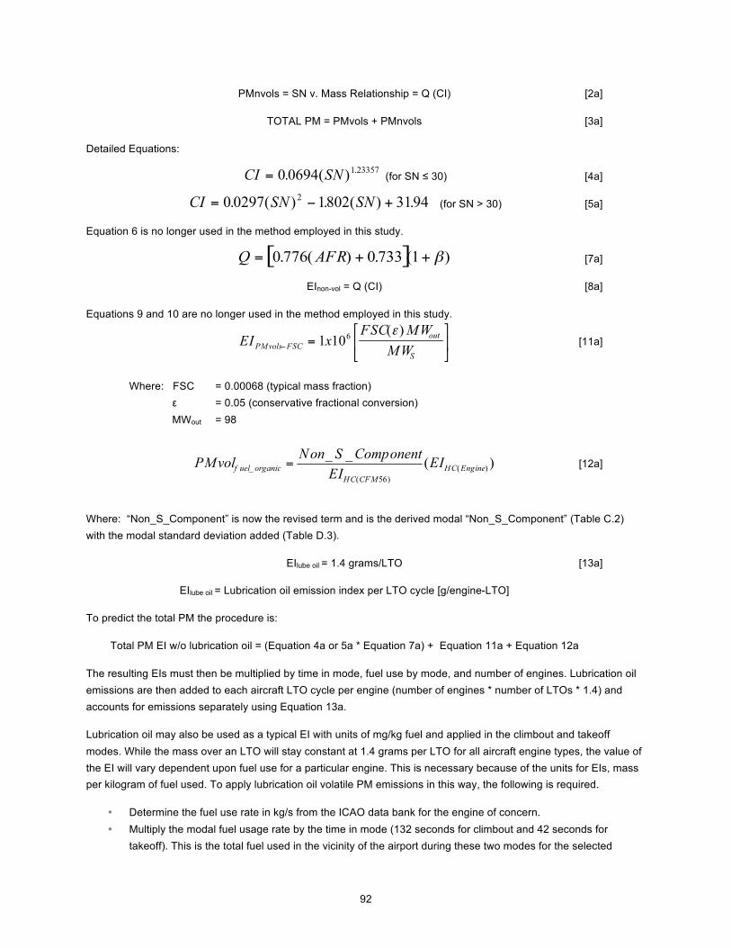
92

PMnvols = SN v. Mass Relationship = Q (CI) [2a]

TOTAL PM = PMvols + PMnvols [3a]

Detailed Equations:

(for SN ≤ 30) [4a]

(for SN > 30) [5a]

Equation 6 is no longer used in the method employed in this study.

[7a]

EInon-vol = Q (CI) [8a]

Equations 9 and 10 are no longer used in the method employed in this study.

[11a]

Where: FSC = 0.00068 (typical mass fraction)

ε = 0.05 (conservative fractional conversion) MWout = 98

[12a]

Where: “Non_S_Component” is now the revised term and is the derived modal “Non_S_Component” (Table C.2) with the modal standard deviation added (Table D.3).

EIlube oil = 1.4 grams/LTO [13a]

EIlube oil = Lubrication oil emission index per LTO cycle [g/engine-LTO]

To predict the total PM the procedure is:

Total PM EI w/o lubrication oil = (Equation 4a or 5a * Equation 7a) + Equation 11a + Equation 12a

The resulting EIs must then be multiplied by time in mode, fuel use by mode, and number of engines. Lubrication oil emissions are then added to each aircraft LTO cycle per engine (number of engines * number of LTOs * 1.4) and accounts for emissions separately using Equation 13a.

Lubrication oil may also be used as a typical EI with units of mg/kg fuel and applied in the climbout and takeoff modes. While the mass over an LTO will stay constant at 1.4 grams per LTO for all aircraft engine types, the value of the EI will vary dependent upon fuel use for a particular engine. This is necessary because of the units for EIs, mass per kilogram of fuel used. To apply lubrication oil volatile PM emissions in this way, the following is required.

Determine the fuel use rate in kg/s from the ICAO data bank for the engine of concern. Multiply the modal fuel usage rate by the time in mode (132 seconds for climbout and 42 seconds for

takeoff). This is the total fuel used in the vicinity of the airport during these two modes for the selected

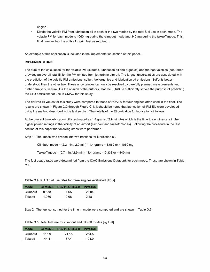
93

engine. Divide the volatile PM from lubrication oil in each of the two modes by the total fuel use in each mode. The

volatile PM for each mode is 1060 mg during the climbout mode and 340 mg during the takeoff mode. This final number has the units of mg/kg fuel as required.

An example of this application is included in the implementation section of this paper.

IMPLEMENTATION

The sum of the calculation for the volatile PM (sulfates, lubrication oil and organics) and the non-volatiles (soot) then provides an overall total EI for the PM emitted from jet turbine aircraft. The largest uncertainties are associated with the prediction of the volatile PM emissions; sulfur, fuel organics and lubrication oil emissions. Sulfur is better understood than the other two. These uncertainties can only be resolved by carefully planned measurements and further analysis. In sum, it is the opinion of the authors, that the FOA3.0a sufficiently serves the purpose of predicting the LTO emissions for use in CMAQ for this study.

The derived EI values for this study were compared to those of FOA3.0 for four engines often used in the fleet. The results are shown in Figure C.2 through Figure C.4. It should be noted that lubrication oil PM EIs were developed using the method described in the last section. The details of the EI derivation for lubrication oil follows.

At the present time lubrication oil is estimated as 1.4 grams / 2.9 minutes which is the time the engines are in the higher power settings in the vicinity of an airport (climbout and takeoff modes). Following the procedure in the last section of this paper the following steps were performed.

Step 1: The mass was divided into two fractions for lubrication oil.

Climbout mode = (2.2 min / 2.9 min) * 1.4 grams = 1.062 or ≈ 1060 mg

Takeoff mode = (0.7 min / 2.9 min) * 1.4 grams = 0.338 or ≈ 340 mg

The fuel usage rates were determined from the ICAO Emissions Databank for each mode. These are shown in Table C.4.

Table C.4: ICAO fuel use rates for three engines evaluated. [kg/s]

Mode CFM56-3 RB211-535E4-B PW4158 Climbout 0.878 1.65 2.004 Takeoff 1.056 2.08 2.481

Step 2: The fuel consumed for the time in mode were computed and are shown in Table D.5.

Table C.5: Total fuel use for climbout and takeoff modes [kg fuel]

Mode CFM56-3 RB211-535E4-B PW4158 Climbout 115.9 217.8 264.5 Takeoff 44.4 87.4 104.0

94

Step 3: The PM volatile mass from lubrication oil emissions for each of the two modes was divided by the fuel consumed in each mode and the final results are shown in Table C.6.

Table C.6: Lubrication oil EIs for climbout and takeoff for selected engines. [mg/kg fuel]

Mode CFM56-3 RB211-535E4-B PW4158 Climbout 9 5 4 Takeoff 8 4 3

These values were included in the overall EIs which are shown in Figure C.2 through Figure D.5.

95

Figure C.2: Comparison of FOA3.0a to FOA 3.0 for the PW4158 engine

Figure C.3: Comparison of FOA3.0a method to FOA 3.0 for the CFM56-3B-2 engine.

96

Figure C.4: Comparison of FOA3.0a method to FOA 3.0 for the RB211-535E4 engine.

97

Figure C.5: Comparison of FOA3.0a method to FOA 3.0 for the GE90-77B engine.

RECOMMENDATIONS

1. For the purposes of this study only, the FOA3a method should be adopted as the current technique to estimate PM emissions from jet turbine aircraft in the vicinity of airports for CMAQ modeling.

2. Separate from this study, efforts should continue to improve the FOA until it can be replaced by measurement data.

98

Appendix D Data Collection and Analysis of Aircraft Auxiliary Power Unit Usage

Prepared by Metron Aviation, Inc.

Background

As discussed in the body of the report, a part of the overall study approach required the collection of usage data for auxiliary power units (APUs). An APU is a relatively small self-contained generator used in aircraft to start the main engines, usually with compressed air. In addition, they provide electrical power and compressed air to operate the aircraft’s instruments, lights, ventilation, and other equipment (typically while the aircraft is parked at the gate). In many aircraft, the APU can also provide electrical power for the aircraft while in the air. In most cases, the APU is powered by a small gas-turbine engine that provides compressed air from within or drives an air compressor.

APUs are routinely used throughout the time an aircraft is on the ground. APU usage is determined by individual airlines and varies with aircraft type and several other factors. For arrivals, some airlines will start the APU when the aircraft is on approach. It will stay on during the entire taxi-in phase to ensure its availability if the engines need to be restarted. Other airlines may operate the APUs during taxi-in if they are using reduced power or a single engine.

During the departure phase of a flight, the APU is used to start the main engine. Some airlines will keep the APU operating during taxi-out as a backup. In addition, when an aircraft is expected to temporarily park away from the gate, the APU will be used during the taxi-out phase of flight.

Factors Affecting APU Usage

APU use varies with aircraft type, airline, and airport. Aircraft size has an influence on the time it takes to service and load the aircraft, and thus influences the time that the APU is utilized. For a given aircraft type, the specific APU used will vary between airlines depending on the equipment onboard the aircraft.. For a particular airline, the APU unit may be used differently at two different airports. Factors such as availability of ground-based power units and airport environment, both climatologically and procedurally, affect the usage of APUs.

The availability of a ground-based power unit affects APU usage in several ways. If a pilot knows a ground-based unit exists at the gate, the APU may remain off during taxi-in time with the understanding that the ground-based unit will power the aircraft at the gate. Even when a ground-based unit is available at the gate, the airline may decide to start the APU during flight preparations.

With regard to airport location, a flight at an airport that is located in a warmer or colder climate will often need to use the APU longer than one operating at an airport in a more temperate location. In addition, APU usage generally increases during the summer and winter months due to increased need for cooling or heating.

There are at least four operational phases to consider when discussing APU use:

Departure Preparations: If ground-based support is available, APUs may be turned on just prior to pushing back from the gate, or, if no ground support is available, the APUs may be started to help prepare the cabin for passengers or cargo.

Departure Taxi: Once the aircraft leaves the gate the carrier may have a standard operating procedure to taxi on fewer than all of the engines. If the engines are not producing the needed power to maintain the cabin environment, the APU may be used as a supplement.

Arrival Taxi: When the aircraft lands and taxis to the gate the APU again may be used to supplement power depending on the use of the aircraft’s engines.

99

Arrival at the Gate: If power and conditioned air are available at the airport’s gate, the APU might remain on until the aircraft is properly connected to the ground source. If no ground support is available, the APU may be shut off or remain operating, depending on when the aircraft will be used next or for maintenance purposes.

APUs also have varying power settings, and therefore differences in resulting emissions per unit of operating time.

Method and Results

When computing emissions associated with flight operations, the FAA Emission and Dispersion Modeling System (EDMS) incorporates estimated APU usage times as part of the calculation. If the user cannot provide more detailed information, EDMS Version 4.11 provides a default APU operation time of 26 minutes per aircraft landing/take-off cycle (LTO), independent of any other factors. In EDMS Version 5.0, certain improvements have been made. In EDMS Version 5.0, APU times are now allocated to arrivals and departures separately to allow for analysis without looking at the entire LTO.

As an initial step toward providing additional information from which to estimate APU usage for this study, APU usage data was collected in a limited, informal fashion from several airlines. We discussed patterns of usage, dependencies on the factors discussed above, and the availability of carrier statistics. In addition to background information from several airlines, quantitative data was provided by three airlines. This quantitative data can be characterized as follows:

Airline A – Partial data for four wide-body types and one narrow body type, covering 4-6 months of operation, but no information on numbers of aircraft or airports sampled. The range of usage for wide-body aircraft during the period was from 1 to 2.3 hours/flight, and 0.9 to 1.4 hours/flight for narrow-body aircraft. Some variation in seasonal use was apparent, with the monthly averages for all aircraft sampled ranging from about 1.1 to 2.0 hours/flight between the lowest-use month and the highest.

Airline B – One year of data for airframes of a single narrow-body type, with the number of airframes sampled each month ranging from 54 to 78. The number of airports serviced was not captured, but was probably substantial. Some variation in seasonal use was apparent, with the monthly averages for all aircraft sampled ranging from about 0.9 to 1.1 hours/flight between the lowest-use month and the highest. Wide variation in usage between airframes was observed, with the yearly average ranging from about 0.3 to 3.4 hours/flight.

Airline C – Average usage times per flight for one narrow-body aircraft and one wide-body aircraft. The amount of data used to develop these averages was not specified.

As contact was made with various carriers it became clear that collection and analysis of APU usage was at different levels of detail and maturity for each airline. Data has not been captured in a consistent fashion and is dependent on ease of availability and on the carrier’s internal needs. Furthermore, although many carriers have standard operating procedures for when and how to use APUs, the ultimate decision rests with the pilot.

Collection of such data is challenging for two reasons. Some airlines believe the data to be proprietary and are reluctant to distribute it. In addition, APU usage data is evidently not trivial to record, and is consequently not recorded by airlines on a regular and systematic basis. Due to these challenges, APU times collected in this initial effort do not distinguish between APU usage during taxi and APU usage at the gate.

However, it should be noted that several airlines contacted were currently performing APU studies themselves to

100

determine how to reduce APU time. As the price of jet fuel continues to rise, it is expected that more airlines will study APU usage and aim to improve efficiency. More systematic data may then become available.

Once the available data was assembled, the aircraft types represented were aggregated into two classes: wide-body and narrow-body jet. In addition, the wide range of the available data was represented by three values of APU usage per LTO cycle in each class: low, moderate, and high. The usage estimates derived from the available data are as follows:

Table D.1: APU use per LTO cycle (minutes)

Narrow Body Wide Body Low Moderate High Low Moderate High 31 48 65 96 130 163

The available data is not sufficiently specific to draw strong conclusions, but an interim approach might be to use the lower values to represent situations in which aircraft have access to ground support, while the upper values could represent situations where ground support is not available. Additional judicious use of these values might represent differences in seasonal use and airport climatic conditions.

Next Steps

To better estimate the usage of APUs at airports, more data and supporting analysis is needed. With the assistance of appropriate trade organizations, additional carriers should be contacted to increase the sample size, as well as the level of detail. It would appear that some carriers are modifying operating practices in this area, and an understanding of trends in these changes should be developed. In addition, airport-oriented data collection could be undertaken to determine the availability of ground-based units, the average time planes are parked somewhere other than at the gate, meteorological conditions through the year, etc. From these types of data, more accurate estimates of APU usage under different conditions, as well as sensitivities to other factors, could be derived.

Effects of Auxiliary Power Units

The baseline inventory described in Section 3.1 provided the basis for the NEI comparison, the air quality modeling, and health impact analysis. This inventory was created assuming a medium level of APU usage. An assessment of the impacts of APUs on LTO emissions was performed, requiring two additional inventories with different APU assumptions. In addition, for evaluation purposes in regard to the 148 airports in non-attainment areas, a total of three emissions inventories were created using the high, medium, and low APU times. These APU inventories were then compared to total aircraft LTO emissions.

Under the low APU usage scenario, the greatest percentage that APUs contributed to total aircraft emissions at an airport was under 10% for CO and between 15 and 20% for NOx and SOx. For the high APU usage scenario, the percentages increased to over 15% for CO and over 30% for NOx and SOx. However, investigating the airports where APU emissions were a high percentage of total LTO emissions revealed that these airports served a higher percentage of business jet operations. For certain small business jets with small taxi times, an hour of APU time (the upper value) can produce enough SOx emissions to account for more than 30% of LTO emissions. This analysis likely overstates the contribution of APU emissions since it may not be realistic to assume that a business jet will spend an hour with the APU operating during an LTO when there is limited loading and unloading of passengers.

101

Additionally, an inventory of all 325 airports with VFR and IFR traffic was created using the medium level of APU usage; the range of contribution of the medium level of APU usage to aircraft emissions below 3,000 feet is between 0% and slightly over 25%, as shown in Figure E.1.82 The average is below 5% for CO and VOCs and under 10% for NOx and SOx. For only four non-attainment areas considered in this report, the medium level of APU usage contributes over 1% to census area emissions (or total emissions) as estimated in the 2002 National Emissions Inventory.

Figure D.1: Range of the percentage of aircraft emissions due to APU at 325 airports studied

In airports with a high volume of operations, the effect of APUs is overshadowed by the emissions from the main engines. However, in areas with fewer operations with less delay, APU emissions play a greater role.

Using data that were generated for Section 4.2, the effects of APU usage were evaluated in a no ground delay scenario. If the aircraft experienced no delay and the APU usage remained the same (currently there is no extra APU usage assumed for periods of delay), then at medium levels of usage APUs would result in more than 15% of the aircraft emissions for CO, greater than 25% for NOx and greater than 30% for SOx. As the system is driven to less ground delay, APUs may play a greater role in aircraft emissions below the mixing height.

82 It is possible for airports to have aircraft that do not have APUs.

102

Appendix E Emissions and Dispersion Modeling System (EDMS) Baseline Aircraft Emissions Inventory

A baseline emissions inventory for all aircraft arriving to and departing from the 325 study airports was generated using aircraft operations data from the most current FAA Enhanced Traffic Management System (ETMS)83 data for the period between June 2005 and May 2006, providing one year of operations for each airport. The operations data was used as input to the FAA Emissions and Dispersion Modeling System (EDMS84), version 5.02 An older version of EDMS was used to generate aircraft emissions inventories for the 2001 EPA National Emissions Inventory; PM emissions factors for this version of EDMS were based on data for several engines in AP 42, which is an EPA compilation of air pollutant emissions factors,85 In contrast, version 5.02 of EDMS contains the FOA3a method for estimating PM emissions from aviation (described in Appendix C), and actual aircraft operational data was used as an input to EDMS version 5.02 to generate aviation emissions estimates for this study. Rather than assuming a particular national mix of engines and airframes, data on specific engine-airframe combinations were used. Additionally, modeled operations were based solely on the data available and were not averaged across months to give annual estimates of emissions. Thus, the aviation emissions data generated by EDMS 5.02 was of a higher fidelity than the aviation emissions data in the 2001 NEI. For this reason, the EDMS emissions inventory was used for this study.

General information on Instrument Flight Rules (IFR) flights was gathered from ETMS.86 ETMS provides the flight number, the origin and destination airport for the flight, and a generic aircraft type. The generic aircraft type is not suitable for modeling emissions; specific airframe and engine combinations are required. The Bureau of Transportation Statistics (BTS) On-Time Performance Database87 was used to match flight numbers to aircraft registration numbers (tail number), in order to match each flight to a specific aircraft type. Over 12.5 million operations were generated by combining these two sources.

Registration information for the aircraft was obtained from the commercially-available BACK fleet database88 or the FAA’s aircraft registration database.89 These databases were used to determine the engine models installed on individual aircraft based on the tail number. The BTS data also provides aircraft pushback, wheels up, touchdown, and gate arrival times. This allowed outbound and inbound taxi times to be calculated for input into EDMS. Since not all flights appear in the BTS data, flights not reported in BTS were assumed to have taxi times equal to the average of the reporting flights at the airport performing a similar operation during the same hour.

The data gathered through ETMS and BTS provided only a portion of the operational profile (IFR traffic). Visual Flight Rules (VFR) traffic operations were estimated by subtracting IFR operations from the total operations for the airport as listed in the Air Traffic Activity Data System (ATADS). The fleet mix of VFR aircraft was estimated from typical aircraft categories based at each airport.

Aircraft operations were aggregated by airframe, engine and takeoff weight to ease the computational requirements 83 http://www.fly.faa.gov/Products/Information/ETMS/etms.html 84 http://www.faa.gov/about/office_org/headquarters_offices/aep/models/edms_model/ 85 http://www.epa.gov/ttn/chief/ap42/ 86 IFR traffic refers to aircraft that operate using an internal mechanism to show visually or aurally the attitude, altitude or operation of the aircraft. These flights include electronic devices for automatically controlling the aircraft in flight. The majority of commercial flights operate under IFR. VFR traffic refers to flights in which the pilot has responsibility for maintaining separation distances visually. VFR flights are mainly performed by general aviation traffic operating small aircraft. 87 http://www.transtats.bts.gov/OT_Delay/OT_DelayCause1.asp 88 http://www.backaviation.com/Information_Services/ 89 Federal Aviation Administration Registry Database, Fall 2006, available from http://registry.faa.gov/.

103

of EDMS. The taxi in and out times were averaged across those operations at an airport level by engine and airframe type. These averages were computed by month. If sufficient engine and airframe data did not exist, default averages for the airport were used; if airport defaults did not exist, ICAO default taxi times were used. To compute an upper bound on aircraft emissions during taxi, all operations were assumed to taxi in and out using all engines for the entire estimated taxi time.90

The FAA registration database and the National Airspace System Resources (NASR)91 were used as additional data sources to help determine VFR operations at airports in nonattainment areas, and the operational profile was fed into EDMS. Inventories were generated for CO, hydrocarbons, NOx, and SOx for all phases of taxi and flight based on International Civil Aviation Organization (ICAO) engine emissions indices—estimates of the mass of pollutant produced per mass of fuel consumed as contained in the International Civil Aviation Organization (ICAO) Engine Emissions Certification Databank.92 To estimate total emissions of particulate matter (PM), a criteria pollutant composed of a complex mixture of solid particles and liquid droplets, EDMS must rely on research-based estimation techniques integrated into EDMS (see Appendix C). Emissions were then aggregated by month and mode for use in the air quality analysis.

Figure E.1: Overview of the generation of the baseline inventory

Inventory Limitations and Sources of Discrepancies

Several generalizations, estimations and approximations were made in creating the baseline inventory that served as

90 Carriers frequently use single engine taxi going to and from terminal gates. Additionally, pilots often shut off main engines and switch to APUs during long delays. The circumstances of single engine taxi use and APU use during extended delays could not be adequately defined for consistent, realistic modeling across the variety of carriers, airports and weather conditions. 91 Federal Aviation Administration, National Airspace System Resources (NASR) data, 2006. 92 http://www.caa.co.uk/default.aspx?catid=702&pagetype=90

104

the basis for the air quality modeling and health impact analysis. These discrepancies were mitigated when possible, but some remain as discussed in this section.

Taxi Times

When available, exact taxi times from BTS data were used. If taxi times were not listed, the average taxi time for the departure/arrival hour at the origin/destination was used. If there were no BTS flights during that hour, the average for the year was used. If annual BTS information was not available for the airport, the ICAO standard time of 19 minutes for taxi-out and 7 minutes for taxi-in was assumed.

Additionally, taxi times were assumed to consist of full engine taxi regardless of the type of aircraft or the length of the taxi time. Anecdotally, it is known that aircraft often taxi-out on one engine and use APUs instead of main engines during long delays, but we chose to create a conservative estimate due to the uncertainty associated with the exact timing of how and when the aircraft may switch to APU or a single engine taxi.

APUs

The APU survey provided information about the range of APU use (see Appendix D). However, the survey was centered on commercial carriers, not business jets. While, commercial aircraft have longer boarding and disembarkment times than business jets, the APU assumptions were applied uniformly to both types of aircraft.

For departing flights, anticipated delays may prompt pilots to shut off main engines and run APUs to conserve fuel. Although airlines have individual operating procedures, the ultimate decision rests with the pilot, making modeling very difficult. The estimates of APU usage do not account for the fact that pilots may turn off main engines and use the APU during periods of long delay.

Default Engines

Engines were matched to air frames based on tail number. However, for some flights, there was no BTS information to provide tail numbers. In addition, some tail numbers did not match specific information in Campbell-Hill, BACK or FAA registration databases. For these aircraft, the EDMS default engine, the most commonly occurring engine for that air frame in the US was used.

International Flights

International flights are not listed in the BTS data set. This limits the specific information available about these flights and requires a greater number of default values for inputs. Default values are particularly problematic as international flights tend to operate heavy aircraft with higher fuel burn. ETMS was used to obtain information on international flights. Because ETMS does not contain taxi data, international flights were assigned airport-level default taxi times when possible. For airports that did not have default taxi times, the ICAO default taxi/idle time was used. Accurately portraying these flights with the correct engines and taxi times is required to more correctly estimate total emissions at international airports.

Particulate Matter Emissions Inventory

The measurement methodology for PM for jet turbine aircraft is still being developed and data are sparse. Measurement and modeling of aircraft PM emissions is still an emerging area and there are data limitations and uncertainties.93,94 A small data set (APEX-195) not used for development of the PM model was used as a

93 The determination of fine particulate matter emissions from aircraft engines is an active area of research. Methods to estimate primary PM emissions from aircraft are relatively immature: test data are sparse, and test methods are

105

comparison to estimate non-volatile confidence limits. Additionally, limits on measurement errors of the independent variable for non-volatile estimation (based on the reported smoke number) were evaluated as well to determine upper and lower bounds of the estimation technique. For the non-volatiles, no direct comparison to measured data was possible due to a lack of data.

The PM emissions inventory contains two known errors: The primary PM inventories for 78 of the 325 study airports were generated using a fuel sulfur emissions index of 0.8 g/kg-fuel burned (corresponding to a fuel sulfur concentration of 400 ppm), versus a value of 1.36 g/kg-fuel burned (corresponding to a fuel sulfur concentration of 680 ppm which is more representative of the current jet fuel supply). The higher fuel sulfur emissions index was used to generate the results in Sections 4 and 5; however, time and resources were not available to repeat the air quality and health effects modeling. The error in the sulfur specification impacted both the volatile component of the primary PM emissions, and the secondary PM precursor emissions. By analyzing the changes in the inventories we estimate that this led to an underestimation of the health effects of approximately 10%. However, this underestimation is approximately offset by the conservatively-biased assumptions in the primary PM inventory estimation method (FOA3a) such that the net effect is that the health effects shown in the body of the report are not biased high or low.

The second problem that occurred was an incorrect factor used for the fuel organics portion of the volatile PM component. (PM emissions include volatile and non-volatile components – see Appendix C.) This was extensively evaluated and found to cause an approximate 3% error. This error is less than the expected uncertainties of the model and calculations show that no changes in the conclusions would occur.

still under development. ICAO and EPA do not have approved test methods or certification standards for aircraft PM emissions. ICAO’s Committee on Aviation Environmental Protection has developed and approved the use of an interim First Order Approximation (FOA3) method to estimate total PM emissions (or total fine PM emissions) from certified aircraft engines. Subsequent to the completion of FOA3, the FOA3 methodology was modified with margins to conservatively account for the potential effects of uncertainties that include the lack of a standard test procedure, poor definition of volatile PM formation in the aircraft plume, and the limited amount of data available on aircraft PM emissions. This modified methodology is known as FOA3a. FOA3a is currently the agreed upon method to estimate total PM emissions from aircraft engines, and it has been incorporated into the latest version of the FAA Emissions and Dispersion Modeling System (EDMS), version 5.02, June 2007. FOA3a was used in this study. FOA3a predicts fine PM inventory levels that are approximately 5 times those predicted by FOA3. The factor of 5 difference between the method used for this study and that determined by the ICAO method reflects the scientific uncertainty associated with PM emissions rates from aircraft engines. 94 In particular, a fuel sulfur level of 400 ppm was assumed for some airports and 680 ppm was assumed for others. Our intention was to assume 680 ppm for all airports. However, year-to-year and location-to-location variations of fuel sulfur of this level (±200 ppm) are typical and are thus within the uncertainty of the estimation methods. 95 Wey, C. C. et al. (2006). Aircraft particle emissions experiment (APEX). NASA TM-2006-214382, National Aeronautics and Space Administration, Washington, DC, September.

106

Appendix F Modeling of the Impact of Aircraft Emissions on Air Quality in Nonattainment Areas

U.S. Environmental Protection Agency

Office of Air Quality Planning and Standards Air Quality Assessment Division

Research Triangle Park, NC

I. Introduction A national scale air quality modeling analysis was performed to estimate the impact of emissions from 325 commercial service airports across the U.S. on annual fine particulate matter (PM2.5) concentrations and daily maximum 8-hour ozone concentrations. These 325 commercial service airports include 148 airports located in nonattainment areas, and 177 airports in attainment areas.96 This document describes the air quality modeling portion of this analysis.

To model the air quality benefits of this rule we used the Community Multiscale Air Quality (CMAQ)97 model. CMAQ simulates the numerous physical and chemical processes involved in the formation, transport, and destruction of ozone and particulate matter. Inputs to the CMAQ model include: emissions estimates (from aircraft and all other sources), meteorological fields, and initial and boundary condition data. For this study, two annual, national CMAQ sensitivity scenarios were modeled focusing on aircraft emissions, one with the specific aircraft emissions (based on 2005 activity at 325 commercial service airports) that were calculated by utilizing FAA’s Emissions and Dispersion Modeling System (EDMS)98 model and one without those emissions. The difference in estimated pollutant concentrations between these two simulations indicates the regional air quality impacts of the aircraft emissions included in the base simulation. These projections were used as inputs to the calculation of health impacts resulting from the 2005 aircraft emissions at the 325 airports. The EDMS modeling99 and the health impact estimation are described in separate documentation100.

II. CMAQ Model Configuration, Inputs, Evaluation, and Methodology

The air quality modeling platform used in this study to estimate the impacts from EDMS aircraft emissions has been used to support several other major regulatory actions initiated by EPA, including:

the final PM2.5 National Ambient Air Quality Standards (NAAQS) regulatory impact analysis101,

96 The 325 airports represent 63 percent (325 of 515) of the commercial service airports in the U.S. 97 Byun, D.W., and K. L. Schere, 2006: Review of the Governing Equations, Computational Algorithms, and Other Components of the Models-3 Community Multiscale Air Quality (CMAQ) Modeling System. Applied Mechanics Reviews, Volume 59, Number 2 (March 2006), pp. 51-77. 98 This study utilized a research version of EDMS 5.0.2, and this version was designed to meet the needs of the study. Documentation about the model is available at http://www.faa.gov/about/office_org/headquarters_offices/aep/models/edms_model/. 99 CSSI, Inc., 2005, Emissions and Dispersion Modeling System (EDMS) User’s Manual, Washington, DC, CSSI, Inc. Prepared for the Federal Aviation Administration Office of Environment and Energy. 100 Abt Associates Inc., 2005, Environmental Benefits Mapping and Analysis Program (BenMAP) User's Manual. Bethesda, MD, Abt Associates, Inc. Prepared for the U.S. Environmental Protection Agency Office of Air Quality and Standards. 101 U.S. Environmental Protection Agency, Final RIA PM NAAQS, Chapter 2: Defining the PM2.5 Air Quality Problem, http://www.epa.gov/ttn/ecas/ria.html, October 2006.

107

the draft 8-hour ozone NAAQS regulatory impact analysis (RIA)102, and the proposed rule for the "Control of Emissions of Air Pollution from Locomotives and Marine Compression-

Ignition Engines Less than 30 Liters per Cylinder"103.

As a result of these previous exercises, EPA is confident in the suitability of this modeling platform for this study. The subsequent sections will describe the model configuration for the base and sensitivity simulations and provide an evaluation of model performance for the base year.

A. Model version The CMAQ model is a three-dimensional grid-based Eulerian air quality model designed to estimate the formation and fate of oxidant precursors, primary and secondary particulate matter concentrations and deposition over regional and urban spatial scales. The CMAQ model was peer-reviewed104 in 2003 for EPA and is a freely-available, non-proprietary model. The latest version of CMAQ available at the time of this study, version 4.5, was employed for this analysis105. This version reflects updates in a number of areas to improve the underlying science and address comments from the peer-review including:

a state-of-the-science inorganic nitrate partitioning module (ISORROPIA) and updated gaseous,

heterogeneous chemistry in the calculation of nitrate formation, a secondary organic aerosol (SOA) module that includes a more comprehensive gas-particle partitioning

algorithm from both anthropogenic and biogenic SOA, an in-cloud sulfate chemistry module that accounts for the nonlinear sensitivity of sulfate formation to varying

pH, and an updated CB-IV gas-phase chemistry mechanism and aqueous chemistry mechanism that provide a

comprehensive simulation of aerosol precursor oxidants. B. Model domain and grid resolution

The CMAQ modeling analyses were performed for a domain covering the majority of the United States (i.e., the lower 48 States), as shown in Figure F.1. This domain has a horizontal grid resolution of 36 km. The use of this relatively coarse resolution limits the analysis to an assessment of regional impacts of the EDMS emissions, as opposed to highly-localized ozone impacts which would require finer resolution modeling. The model extends vertically from the surface to 100 millibars (approximately 15,674 meters above sea level) using a sigma-pressure coordinate system consisting of 14 vertical layers. The model domain uses a Lambert Conformal map projection with true latitudes at 33 and 45 degrees N. The center of the domain is at latitude 40 N, longitude 97 W. The dimensions of the modeling grid are 148 columns by 112 rows.

102 U.S. Environmental Protection Agency, Regulatory Impact Analysis of the Proposed Revisions to the National Ambient Air Quality Standards for Ground-Level Ozone, http://www.epa.gov/ttn/ecas/ria.html#ria2007 July 2007. 103 U.S. Environmental Protection Agency; Technical Support Document for the Proposed Locomotive-Marine Rule: Air Quality Modeling; Office of Air Quality Planning and Standards; EPA 454/R-07-004; RTP, NC; March 2007 104 Amar, P., R. Bornstein, H. Feldman, H. Jeffries, D. Steyn, R. Yamartino, and Y. Zhang. 2004. Final Report Summary: December 2003 Peer Review of the CMAQ Model, pp. 7. 105 U.S. Environmental Protection Agency, Community Multiscale Air Quality (CMAQ), http://www.epa.gov/asmdnerl/CMAQ/release45.html, January 2009.

108

Figure F.1: Map of the CMAQ modeling domain. The box outlined in black denotes the 36 km modeling domain.

C. Modeling Period

There are several considerations involved in selecting the appropriate duration of an air quality modeling analysis106. In general, the goal is to model several types of meteorological conditions that lead to ambient PM2.5 levels and ozone levels similar to an area’s design value107. For the annual PM2.5 standard, it was determined that modeling an entire year of meteorology (2001) was needed to estimate the impacts of the EDMS emissions upon annual average levels of PM2.5, because seasonal changes in atmospheric composition and meteorology affect the final annual average PM2.5 values. For the 8-hour ozone standard, we only used the simulation days within the May through September 2001 period to estimate the impacts of the aircraft sector, as only several days of simulation are needed to determine 8-hour ozone values and May through September is the typical ozone season in the continental United States.108 Over most parts of the U.S., this period should be sufficient to capture typical conditions that lead to high

106 U.S. EPA, Guidance on the Use of Models and Other Analyses in Attainment Demonstrations for the 8- hour Ozone NAAQS; EPA-454/R-05-002; Research Triangle Park, NC; October 2005. 107 A design value is a statistic, specific to a given criteria pollutant and based on measurements of the concentration of that pollutant in the local atmosphere of a given area, that describes the air quality status of a given area relative to the level of the National Ambient Air Quality Standards (NAAQS) for that criteria pollutant. The methodologies for deriving design values for ozone and PM2.5 are contained in 40 CFR 50 Appendix H and 40 CFR 50 Appendix N, respectively. Historical design values can be found at http://www.epa.gov/airtrends/values.html. 108 U.S. EPA, Guidance on the Use of Models and Other Analyses for Demonstrating Attainment of Air Quality Goals for Ozone, PM2.5, and Regional Haze; EPA-454/B-07-002; Research Triangle Park, NC; April 2007.

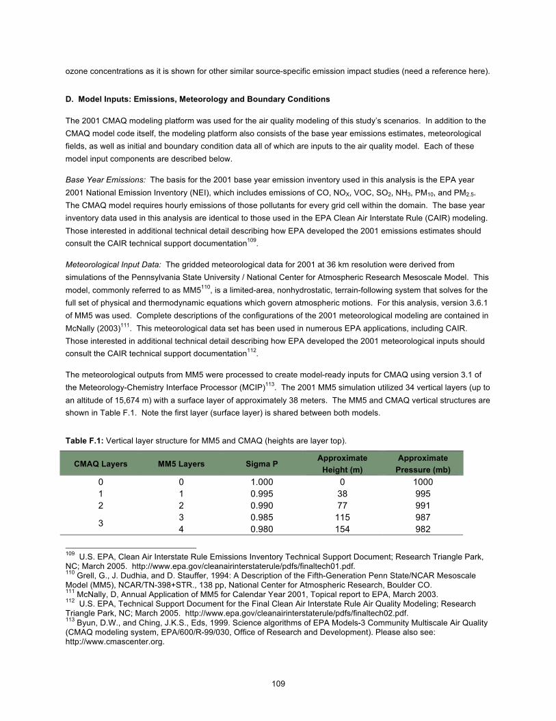
109

ozone concentrations as it is shown for other similar source-specific emission impact studies (need a reference here).

D. Model Inputs: Emissions, Meteorology and Boundary Conditions The 2001 CMAQ modeling platform was used for the air quality modeling of this study’s scenarios. In addition to the CMAQ model code itself, the modeling platform also consists of the base year emissions estimates, meteorological fields, as well as initial and boundary condition data all of which are inputs to the air quality model. Each of these model input components are described below.

Base Year Emissions: The basis for the 2001 base year emission inventory used in this analysis is the EPA year 2001 National Emission Inventory (NEI), which includes emissions of CO, NOX, VOC, SO2, NH3, PM10, and PM2.5. The CMAQ model requires hourly emissions of those pollutants for every grid cell within the domain. The base year inventory data used in this analysis are identical to those used in the EPA Clean Air Interstate Rule (CAIR) modeling. Those interested in additional technical detail describing how EPA developed the 2001 emissions estimates should consult the CAIR technical support documentation109.

Meteorological Input Data: The gridded meteorological data for 2001 at 36 km resolution were derived from simulations of the Pennsylvania State University / National Center for Atmospheric Research Mesoscale Model. This model, commonly referred to as MM5110, is a limited-area, nonhydrostatic, terrain-following system that solves for the full set of physical and thermodynamic equations which govern atmospheric motions. For this analysis, version 3.6.1 of MM5 was used. Complete descriptions of the configurations of the 2001 meteorological modeling are contained in McNally (2003)111. This meteorological data set has been used in numerous EPA applications, including CAIR. Those interested in additional technical detail describing how EPA developed the 2001 meteorological inputs should consult the CAIR technical support documentation112.

The meteorological outputs from MM5 were processed to create model-ready inputs for CMAQ using version 3.1 of the Meteorology-Chemistry Interface Processor (MCIP)113. The 2001 MM5 simulation utilized 34 vertical layers (up to an altitude of 15,674 m) with a surface layer of approximately 38 meters. The MM5 and CMAQ vertical structures are shown in Table F.1. Note the first layer (surface layer) is shared between both models.

Table F.1: Vertical layer structure for MM5 and CMAQ (heights are layer top).

CMAQ Layers MM5 Layers Sigma P Approximate

Height (m) Approximate

Pressure (mb) 0 0 1.000 0 1000 1 1 0.995 38 995 2 2 0.990 77 991

3 0.985 115 987 3 4 0.980 154 982

109 U.S. EPA, Clean Air Interstate Rule Emissions Inventory Technical Support Document; Research Triangle Park, NC; March 2005. http://www.epa.gov/cleanairinterstaterule/pdfs/finaltech01.pdf. 110 Grell, G., J. Dudhia, and D. Stauffer, 1994: A Description of the Fifth-Generation Penn State/NCAR Mesoscale Model (MM5), NCAR/TN-398+STR., 138 pp, National Center for Atmospheric Research, Boulder CO. 111 McNally, D, Annual Application of MM5 for Calendar Year 2001, Topical report to EPA, March 2003. 112 U.S. EPA, Technical Support Document for the Final Clean Air Interstate Rule Air Quality Modeling; Research Triangle Park, NC; March 2005. http://www.epa.gov/cleanairinterstaterule/pdfs/finaltech02.pdf. 113 Byun, D.W., and Ching, J.K.S., Eds, 1999. Science algorithms of EPA Models-3 Community Multiscale Air Quality (CMAQ modeling system, EPA/600/R-99/030, Office of Research and Development). Please also see: http://www.cmascenter.org.

110

CMAQ Layers MM5 Layers Sigma P Approximate

Height (m) Approximate

Pressure (mb) 5 0.970 232 973 4 6 0.960 310 964 7 0.950 389 955 5 8 0.940 469 946 9 0.930 550 937

10 0.920 631 928 6 11 0.910 712 919 12 0.900 794 910 13 0.880 961 892 7 14 0.860 1,130 874 15 0.840 1,303 856 16 0.820 1,478 838 8 17 0.800 1,657 820 18 0.770 1,930 793 9 19 0.740 2,212 766 20 0.700 2,600 730 10 21 0.650 3,108 685 22 0.600 3,644 640 11 23 0.550 4,212 595 24 0.500 4,816 550 25 0.450 5,461 505 12 26 0.400 6,153 460 27 0.350 6,903 415 28 0.300 7,720 370 29 0.250 8,621 325

13

30 0.200 9,625 280 31 0.150 10,764 235 32 0.100 12,085 190 33 0.050 13,670 145 14

34 0.000 15,674 100

Initial and Boundary Conditions: The lateral boundary and initial species concentrations are provided by a three-dimensional global atmospheric chemistry model, the GEOS-CHEM114 model. The global GEOS-CHEM model simulates atmospheric chemical and physical processes driven by assimilated meteorological observations from the NASA’s Goddard Earth Observing System (GEOS). This model was run for 2001 with a grid resolution of 2.0 degree x 2.5 degree (latitude-longitude) and 20 vertical layers. The predictions were used to provide one-way dynamic boundary conditions at three-hour intervals and an initial concentration field for the CMAQ simulations.

E. CMAQ Modeling Scenarios

The CMAQ modeling system was used to estimate annual PM2.5 concentrations, daily 8-hour ozone concentrations, and visibility estimates for four emissions scenarios:

1. a 2001 base case

114 Yantosca, B., 2004. GEOS-CHEMv7-01-02 User’s Guide, Atmospheric Chemistry Modeling Group, Harvard University, Cambridge, MA, October 15, 2004.

111

2. a 2001 base line, 3. a 2001 “no_aircraft” base case with all emissions from the EPA year 2001 National Emissions Inventory

aircraft sectors removed, and 4. scenario #2 with EPA year 2001 National Emissions Inventory aircraft sector emissions removed and

replaced with the EDMS emissions from 325 commercial service airports. The 2001 base case (scenario #1) was modeled in order to evaluate the performance of the CMAQ model and as such included day-specific emissions wherever possible. The results of this evaluation are described in the next section. The 2001 base line simulation (scenario #2) was modeled to serve as a comparison for the two aircraft sensitivity scenarios #3 and #4 based on EPA methodology for applying CMAQ to estimate the impacts of source emissions on ambient ozone and PM2.5 concentrations; see section G of this Appendix. The base line simulation does not include emissions specific to particular days in 2001. For the "no_aircraft" simulation (sensitivity scenario #3) we removed emissions from six source classification categories (SCCs) contained in the EPA year 2001 National Emissions Inventory:

2275000000 Mobile Sources Aircraft All Types and Operations 2275001000 Mobile Sources Aircraft Military Aircraft 2275020000 Mobile Sources Aircraft Commercial Aircraft 2275050000 Mobile Sources Aircraft General Aviation 2275060000 Mobile Sources Aircraft Air Taxi 2275070000 Mobile Sources Aircraft Auxiliary Power Units

For the fourth scenario, we added 2005 commercial service aircraft emissions from the EDMS model as provided by CSSI, Inc115. These emissions capture 95 percent of nationwide activity of aircraft with engines certified to the International Civil Aviation Organization (ICAO) emission standards (specifically, those with ICAO smoke numbers), at commercial service airports116. Also, as described earlier, the 325 airports represent 63 percent (325 of 515) of the commercial service airports in the U.S. The EDMS emissions were provided for CO, VOC, SO2, NOx, primary PM2.5, and three PM2.5 species (sulfates, organic carbon, and elemental carbon). Monthly emissions were provided for seven operating modes: engine startup, auxiliary power units (APUs) , aircraft taxiing in, aircraft taxiing out, takeoff w/ initial climb, climb out, and approach mode, for each of the 325 airports. The aircraft emissions from the seven operating modes were allocated to CMAQ layers (shown in Table F.1), as follows:117

Engine startup: CMAQ layer 1 APUs: CMAQ layer 1 Aircraft Taxi (in): CMAQ layer 1 Aircraft Taxi (out): CMAQ layer 1 Takeoff w/ initial climb: emissions equally divided between layers 1 – 5 Climb out: emissions equally divided between layers 6 – 7 Approach mode: emissions equally divided between layers 1 – 7

115 CSSI, Inc., 2005, Emissions and Dispersion Modeling System (EDMS) User’s Manual, Washington, DC, CSSI, Inc. Prepared for the Federal Aviation Administration Office of Environment and Energy. 116 ICAO emission standards apply to aircraft gas turbine engines with thrust greater than 26.7 kN, which includes engines on commercial single-aisle, twin-aisle, and larger aircraft as well as small regional jets (and some business jets). 117 Aircraft emissions should ideally be allocated to CMAQ layers based on layer thickness and how much time is spent by an aircraft within a given CMAQ layer.

112

Table F.2 shows the relative proportion of CO, NOx, VOC, PM2.5, and SO2 emissions from the EDMS aircraft to the overall base line emissions inventory of all sources nationally, and for 12 select areas (i.e., the areas with the largest PM2.5 contribution from this sector). On a national average level, the EDMS aircraft emissions represent a relatively small percentage of the national PM2.5, PM2.5 precursor, and ozone precursor emissions. However, the percentage contributions can be larger in individual metropolitan areas, based on the amount of aviation emissions vs. the amount of emissions from other sources in those metropolitan areas.

Table F.2: Ratios of EDMS emissions to overall base line (scenario #2) emissions averaged nationally, and for the 12 cities with the largest modeled PM2.5 impact from EDMS aircraft emissions.

Area % CO % NOX % VOC % SO2 % PM2.5 Los Angeles 0.34 % 1.00 % 0.42 % 1.84 % 0.18 % Atlanta 0.42 % 1.59 % 0.65 % 0.25 % 0.17 % Las Vegas 1.39 % 2.80 % 1.44 % 0.35 % 0.36 % Denver 0.41 % 1.53 % 0.86 % 0.64 % 0.20 % Memphis 0.80 % 2.38 % 1.85 % 0.43 % 0.41 % San Francisco 0.33 % 1.53 % 0.47 % 1.15 % 0.14 % Detroit 0.19 % 0.60 % 0.39 % 0.11 % 0.18 % New York City 0.38 % 1.36 % 0.49 % 0.36 % 0.29 % Louisville 0.45 % 0.71 % 1.33 % 0.06 % 0.27 % Minneapolis 0.30 % 1.03 % 0.49 % 0.21 % 0.15 % Salt Lake City 0.53 % 1.27 % 0.63 % 0.49 % 0.20 % Philadelphia 0.31 % 0.72 % 0.41 % 0.10 % 0.16 % National Average118 0.17 % 0.40 % 0.23 % 0.06 % 0.03 % F. CMAQ Base Case Model Performance Evaluation 1. PM2.5: An operational model performance evaluation for PM2.5 and its related speciated components (e.g., sulfate, nitrate, elemental carbon, organic carbon, etc.) was conducted using the base case (scenario #1) simulation data in order to estimate the ability of the CMAQ modeling system to replicate PM2.5 and PM2.5 species concentrations. In summary, model performance statistics were calculated for observed/predicted pairs of daily, monthly, seasonal, and annual concentrations. Statistics were generated for the following geographic groupings: domain wide, Eastern U.S, and Western U.S. (divided based on the 100th meridian). The “acceptability” of model performance was judged by comparing our CMAQ 2001 performance results to the range of performance found in regional PM2.5 model applications for certain other, non-EPA studies119. Overall, the fractional bias (FB), fractional error (FE), normalized mean bias (NMB), and normalized mean error (NME) statistics shown in Table F.3 are within the range or close to that found by other groups in certain other applications.120 The model performance results give us confidence that our application of CMAQ using this modeling platform provides a scientifically credible approach for assessing PM2.5 concentrations for the purposes of this study. A more detailed summary of the CMAQ model performance evaluation

118 The national average was determined by averaging emissions of a given pollutant (according to the 2001 EPA NEI) across all sources in the continental United States. 119 See Appendix C of the CMAQ Model Performance Evaluation Report for 2001 updated March 2005 (CAIR Docket OAR-2005-0053-2149). These other modeling studies represent a wide range of modeling analyses which cover various models, model configurations, domains, years and/or episodes, chemical mechanisms, and aerosol modules. 120 Note that aircraft gas turbine engines do not emit ammonia or PM10.

113

for PM2.5 is available within the PM NAAQS RIA, Appendix O121.

Table F.3: Annual CMAQ 2001 model performance statistics for 2001 base case (scenario #1)

Pollutant Measurement Network Region # of Obs FB (%) FE (%) NMB(%) NME(%)

National 6356 -10 42 -8 39 East 5124 -5 39 -2 35 STN122 West 1232 -29 53 -36 54

National 13218 -11 51 -11 47 East 5606 -11 47 -11 41

PM2.5 Total Mass

IMPROVE123 West 7612 -10 54 -12 55

National 6723 -16 45 -13 36 East 5478 -8 41 -9 34 STN West 1245 -52 64 -51 58

National 13477 -21 50 -20 39 East 5657 -15 41 -16 34 IMPROVE West 7790 -26 57 -33 52

National 3791 -29 37 -21 27 East 2784 -22 29 -19 25

Sulfate

CASTNet124 West 1007 -47 59 -45 51

National 5883 -39 89 -15 74 East 4673 -23 81 14 70 STN West 1210 -103 116 -76 82

National 13398 -72 116 -10 86 East 5636 -53 109 16 90

Nitrate

IMPROVE West 7762 -85 121 -42 82

National 3788 4 38 9 35 East 2781 13 34 14 33

Total Nitrate (NO3 + HNO3) CASTNet

West 1007 -21 51 -27 47 National 6723 20 63 6 54

East 5478 27 59 16 51 STN West 1245 13 78 -53 75

National 3791 -17 38 -11 31 East 2784 -8 32 -10 29

Ammonium

CASTNet West 1007 -39 57 -37 51

National 6842 19 60 22 69 East 5551 26 59 34 71 STN West 1291 -8 65 -13 63

National 13441 -15 60 -2 63 East 5646 -26 53 -18 46

Elemental Carbon

IMPROVE West 7795 -7 66 19 85

National 6685 -46 65 -43 54 East 5401 -45 65 -41 51 STN West 1284 -46 68 -47 61

National 13428 6 63 4 68 East 5658 -28 60 -24 51

Organic Carbon

IMPROVE West 7770 31 64 38 88

121 U.S. EPA, Final RIA PM NAAQS, Appendix O: CMAQ Model Performance Evaluation for 2001. October 2006. http://www.epa.gov/ttn/ecas/regdata/RIAs/Appendix%20O--Model%20Eval.pdf 122 EPA’s Speciation Trends Network, which monitors PM2.5 species. http://epa.gov/ttn/amtic/specgen.html 123 The Interagency Monitoring of Protected Visual Environments network, which monitors visibility in specific National Parks and Wilderness Areas in the U.S. http://vista.cira.colostate.edu/improve/ 124 The Clean Air Status and Trends Network, which aids in assessment of acid deposition. http://www.epa.gov/CASTNET/

114

2. Ozone: Performance for the 36 km ozone modeling was calculated over the period from May 1 to September 30, 2001. Over 1000 ozone monitoring sites were used in these model-to-monitor comparisons. Table F.4 lists the average monthly NMB and NME values for daily maximum 8-hourly ozone over the 36 km domain. This statistical comparison only looks at observed values greater than 60 ppb, in order to focus on the upper end of the observed ozone spectrum that are of most significance from a regulatory perspective.125 The model generally tends to underestimate daily 8-hour ozone peaks on the order of 3-13 percent when averaged over individual months.

Table F.4: CMAQ 8-hourly daily maximum ozone model performance statistics calculated for a threshold of 60 ppb over the entire 36 km domain for 2001.

NMB (%) NME (%)

May -3.0 12.3

June -3.8 12.4

July -10.6 15.7

August -10.3 15.5

September -12.6 16.3

Table F.5 lists the average monthly NMB and NME values for daily maximum 8-hourly ozone over specific subdomains within the 36 km domain. While the resolution is less than ideal for an ozone impact analysis it is encouraging that the operational performance statistics are within the range of certain other regional modeling applications such as CAIR.

Table F.5: CMAQ 8-hourly daily maximum ozone model performance statistics (NMB and NME) calculated for specific subdomains and using a threshold of 60 ppb over the entire domain for 2001.

Central Regional Air

Planning Association

(CENWRAP)126

Lake Michigan Air Directors Consortium (LADCO)127

Mid-Atlantic/Northeast

Visibility Union (MANE-VU)128

Visibility Improvement

State and Tribal

Association of the Southeast

(VISTAS)129

Western Regional Air Partnership (WRAP)130

May -1.8 / 11.5 0.6 / 11.3 -1.7 / 9.9 -5.9 / 11.1 -2.4 / 15.3

June -4.2 / 11.8 -0.2 / 10.5 -3.2 / 11.3 -0.7 / 10.3 -9.8 / 17.1

July -9.8 / 14.1 -7.2 / 14.3 -4.5 / 13.3 -7.4 / 12.5 -19.3 / 21.3

125 U.S. EPA, Guidance on the Use of Models and Other Analyses for Demonstrating Attainment of Air Quality Goals for Ozone, PM2.5, and Regional Haze; EPA-454/B-07-002; Research Triangle Park, NC; April 2007. 126 Includes nine states - Nebraska, Kansas, Oklahoma, Texas, Minnesota, Iowa, Missouri, Arkansas, and Louisiana. 127 Includes five states - Illinois, Indiana, Michigan, Ohio, and Wisconsin. 128 Includes Connecticut, Delaware, the District of Columbia, Maine, Maryland, Massachusetts, New Hampshire, New Jersey, New York, Pennsylvania, Rhode Island, Vermont, Northern Virginia, and suburbs of Washington, D.C. 129 Member States and Tribes include: the States of Alabama, Florida, Georgia, Kentucky, Mississippi, North Carolina, South Carolina, Tennessee, Virginia, and West Virginia and the Eastern Band of the Cherokee Indians. 130 Includes the states of Alaska, Arizona, California, Colorado, Idaho, Montana, New Mexico, North Dakota, Oregon, South Dakota, Utah, Washington, and Wyoming. Also includes Tribes of the Campo Band of Kumeyaay Indians, Confederated Salish and Kootenai Tribes, Cortina Indian Rancheria, Hopi Tribe, Hualapai Nation of the Grand Canyon, Native Village of Shungnak, Nez Perce Tribe, Northern Cheyenne Tribe, Pueblo of Acoma, Pueblo of San Felipe, and Shoshone-Bannock Tribes of Fort Hall.

115

Central Regional Air

Planning Association

(CENWRAP)126

Lake Michigan Air Directors Consortium (LADCO)127

Mid-Atlantic/Northeast

Visibility Union (MANE-VU)128

Visibility Improvement

State and Tribal

Association of the Southeast

(VISTAS)129

Western Regional Air Partnership (WRAP)130

August -10.2 / 14.7 -2.4 / 11.3 -9.6 / 15.3 -5.7 / 11.3 -17.1 / 20.6

September -15.6 / 18.4 -8.7 / 12.5 -13.7 / 15.0 -9.5 / 12.3 -15.9 / 18.0

G. Applications of CMAQ Modeling Output

Model predictions are used in a relative sense to estimate scenario-specific design values of PM2.5 and ozone. This is done by calculating the simulated air quality ratios between any particular sensitivity simulation (e.g., the no_aircraft scenario #3) and the 2001 base line (scenario #2). These predicted change ratios are then applied to ambient base year design values to predict the impact of the source emissions of interest (e.g. EDMS aircraft emissions) upon ambient air quality, quantified as a change in pollutant concentration in µg/m3 (for PM2.5) or ppb (for ozone). These quantified changes are then used as inputs to the health and welfare impact functions of the benefits analysis. The design value projection methodology used in this analysis is standard protocol and followed EPA guidance documentation131 for such analyses. The methodology is described below; see the guidance documentation for further details.

Projection Methodology for Annual Average PM2.5 Design Values: The projected annual design values were calculated using the Speciated Modeled Attainment Test (SMAT) approach. This approach is used to ensure that the PM2.5 concentrations are closely related to the observed ambient data. The SMAT procedure combines absolute concentrations of ambient data with the relative change in PM species from the CMAQ model. The SMAT uses a Federal Reference Method (FRM) mass construction methodology that results in reduced nitrates (relative to the amount measured by routine speciation networks), higher mass associated with sulfates (reflecting water included in FRM measurements), and a measure of organic carbonaceous mass that is derived from the difference between measured PM2.5 and its noncarbon components. This characterization of PM2.5 mass also reflects elemental carbon, crustal material and other minor constituents. The resulting characterization provides a complete mass balance. The SMAT methodology uses the following PM2.5 species components from the FRM construction methodology as inputs: sulfates, nitrates, ammonium, organic carbon mass, elemental carbon, crustal, water, and blank mass (a fixed value of 0.5 µg/m3). More complete details of the SMAT procedures used in this analysis can be found in the revised SMAT procedure for CAIR report132. Below are the steps we followed for projecting scenario-specific PM2.5 concentrations. These steps were performed to estimate sensitivity case concentrations at each FRM monitoring site. The starting point for these projections is a 5 year weighted average design value for each site, based on measurements of total ambient PM2.5 concentrations at each FRM monitoring site. The weighted average is calculated as the average of the 1999–2001, 2000–2002, and 2001–2003 design values at each monitoring site. This approach has the desired benefits of (1) weighting the PM2.5 values towards the middle year of the five-year period (2001), which is the base year for the emissions projections, and (2) smoothing out the effects of year-to-year variability in emissions and meteorology that occurs over the full five-year period of monitoring.

131 U.S. EPA, Guidance on the Use of Models and Other Analyses in Attainment Demonstrations for the 8-hour Ozone NAAQS; EPA-454/R-05-002; Research Triangle Park, NC; October 2005. 132 U.S. EPA, Procedures for Estimating Future PM2.5 Values for the CAIR Final Rule by Application of the (Revised) Speciated Modeled Attainment Test (SMAT), 2004. http://www.epa.gov/interstateairquality/pdfs/Revised-SMAT.pdf.

116

Step 1: Calculate quarterly mean ambient concentrations for each of the major components of PM2.5 (i.e., sulfate, nitrate, ammonium, elemental carbon, organic carbon, water, and crustal material) using the component species concentrations estimated for each FRM site. Because not all FRM sites have co-located speciation monitors, the component species concentrations were estimated using an average of 2002 and 2003 ambient data from EPA speciation monitors, which was the speciation data available at the time. The speciation data was interpolated to provide estimates for all FRM sites across the country. The interpolated component concentration information was used to calculate species fractions at each FRM site. The estimated fractional composition of each species (by quarter) was then multiplied by the 5-year weighted average 1999–2003 FRM quarterly mean concentrations at each site (e.g., 20% sulfate multiplied by 15.0 µg/m3 of PM2.5 equals 3 µg/m3 sulfate). The end result is a quarterly concentration for each of the PM2.5 species at each FRM site.

Step 2: Calculate quarterly average Relative Reduction Factors (RRFs) for sulfate, nitrate, elemental carbon, organic carbon, and crustal material.133 The species-specific RRFs for the location of each FRM are the ratio of quarterly average model predicted species concentrations between the sensitivity cases (i.e., #3 "no_aircraft" and #4 "EDMS") and the base line (scenario #2) simulation. The species-specific quarterly RRFs are then multiplied by the corresponding 1999–2003 quarterly species concentration from Step 1. The result is the scenario case quarterly average concentration for each of these species for each sensitivity scenario.

Step 3: Calculate sensitivity case quarterly average concentrations for ammonium and particle-bound water. The "no_aircraft" and "EDMS" case concentrations for ammonium are calculated using the sensitivity case sulfate and nitrate concentrations determined from Step 2 along with the degree of neutralization of sulfate (held constant from the base year). Concentrations of particle-bound water are calculated using an empirical equation using concentrations of sulfate, nitrate, and ammonium as inputs.

Step 4: Calculate the mean of the four quarterly average sensitivity case concentrations to estimate the annual average concentration for each component species. The annual average concentrations of the components are added together to obtain the annual average concentration for PM2.5 in the sensitivity cases.

Step 5: For counties with only one monitoring site, the projected value at that site is the projected value for that county. For counties with more than one monitor, the highest value in the county is selected as the concentration for that county.

Change in Annual Average PM2.5 for the Benefits Calculations: For the purposes of projecting sensitivity case PM2.5 concentrations for input to the benefits calculations, we applied the SMAT procedure using the 2001 base line modeling scenario (scenario #2) and both of the sensitivity scenarios #3 and #4. The SMAT procedures for calculating PM benefits are the same as documented above.

Projection Methodology for 8-hour Ozone Design Values: For the purpose of estimating impacts on 8-hour ozone design values due to EDMS aircraft emissions, a similar relative approach was used as described above. Relative reduction factors (sensitivity / baseline) were calculated for each model grid cell that contains an ozone monitor for each of the two sensitivity scenarios. These RRF values were calculated using methodology prescribed in existing

133 Note that aircraft gas turbine engines emit crustal material only in trace amounts (e.g. small bits of metal due to engine wear).

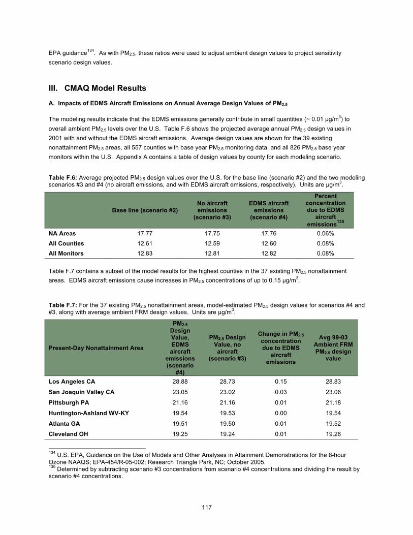
117

EPA guidance134. As with PM2.5, these ratios were used to adjust ambient design values to project sensitivity scenario design values.

III. CMAQ Model Results

A. Impacts of EDMS Aircraft Emissions on Annual Average Design Values of PM2.5 The modeling results indicate that the EDMS emissions generally contribute in small quantities (~ 0.01 µg/m3) to overall ambient PM2.5 levels over the U.S. Table F.6 shows the projected average annual PM2.5 design values in 2001 with and without the EDMS aircraft emissions. Average design values are shown for the 39 existing nonattainment PM2.5 areas, all 557 counties with base year PM2.5 monitoring data, and all 826 PM2.5 base year monitors within the U.S. Appendix A contains a table of design values by county for each modeling scenario.

Table F.6: Average projected PM2.5 design values over the U.S. for the base line (scenario #2) and the two modeling scenarios #3 and #4 (no aircraft emissions, and with EDMS aircraft emissions, respectively). Units are µg/m3.

Base line (scenario #2) No aircraft emissions

(scenario #3)

EDMS aircraft emissions

(scenario #4)

Percent concentration due to EDMS

aircraft emissions135

NA Areas 17.77 17.75 17.76 0.06%

All Counties 12.61 12.59 12.60 0.08% All Monitors 12.83 12.81 12.82 0.08% Table F.7 contains a subset of the model results for the highest counties in the 37 existing PM2.5 nonattainment areas. EDMS aircraft emissions cause increases in PM2.5 concentrations of up to 0.15 µg/m3.

Table F.7: For the 37 existing PM2.5 nonattainment areas, model-estimated PM2.5 design values for scenarios #4 and #3, along with average ambient FRM design values. Units are µg/m3.

Present-Day Nonattainment Area

PM2.5 Design Value, EDMS aircraft

emissions (scenario

#4)

PM2.5 Design Value, no aircraft

(scenario #3)

Change in PM2.5 concentration due to EDMS

aircraft emissions

Avg 99-03 Ambient FRM PM2.5 design

value

Los Angeles CA 28.88 28.73 0.15 28.83

San Joaquin Valley CA 23.05 23.02 0.03 23.06

Pittsburgh PA 21.16 21.16 0.01 21.18

Huntington-Ashland WV-KY 19.54 19.53 0.00 19.54

Atlanta GA 19.51 19.50 0.01 19.52

Cleveland OH 19.25 19.24 0.01 19.26

134 U.S. EPA, Guidance on the Use of Models and Other Analyses in Attainment Demonstrations for the 8-hour Ozone NAAQS; EPA-454/R-05-002; Research Triangle Park, NC; October 2005. 135 Determined by subtracting scenario #3 concentrations from scenario #4 concentrations and dividing the result by scenario #4 concentrations.

118

Present-Day Nonattainment Area

PM2.5 Design Value, EDMS aircraft

emissions (scenario

#4)

PM2.5 Design Value, no aircraft

(scenario #3)

Change in PM2.5 concentration due to EDMS

aircraft emissions

Avg 99-03 Ambient FRM PM2.5 design

value

Birmingham AL 19.05 19.04 0.00 19.05

Cincinnati OH 18.52 18.48 0.04 18.55

Steubenville-Weirton OH-WV 18.36 18.36 0.00 18.36

Knoxville TN 18.09 18.08 0.01 18.11

Chicago IL 17.99 17.97 0.02 18.00

Canton OH 17.84 17.84 0.01 17.85

Charleston, WV 17.74 17.73 0.01 17.75

New York City, NY-NJ-CT 17.54 17.50 0.03 17.56

St. Louis, MO-IL 17.40 17.39 0.01 17.41

Columbus, OH 17.28 17.27 0.01 17.28

Chattanooga, TN-GA 17.23 17.22 0.01 17.24

Baltimore, MD 17.11 17.10 0.01 17.12

Louisville, KY-IN 17.08 17.04 0.04 17.08

Lancaster, PA 16.99 16.98 0.01 16.99

Indianapolis, IN 16.87 16.84 0.02 16.88

Parkersburg-Marietta, WV-OH 16.88 16.87 0.00 16.88

York, PA 16.69 16.68 0.01 16.70

Greensboro, NC 16.56 16.56 0.00 16.56

Macon, GA 16.42 16.42 0.01 16.43

Philadelphia, PA-NJ-DE 16.40 16.36 0.04 16.42

Washington, DC-MD-VA 16.23 16.21 0.02 16.25

Libby, MT 16.25 16.24 0.00 16.25

Reading, PA 16.24 16.23 0.01 16.24

Hickory, NC 16.20 16.19 0.00 16.20

Martinsburg, WV-MD 16.18 16.18 0.00 16.18

Wheeling, WV-OH 16.07 16.06 0.00 16.07

Evansville, IN-KY 16.03 16.02 0.00 16.03

Dayton, OH 15.74 15.72 0.01 15.75

Johnstown, PA 15.62 15.62 0.00 15.63

Harrisburg, PA 15.60 15.60 0.00 15.60

Detroit, MI 15.34 15.32 0.02 15.34

The greatest impacts from the emissions in question tend to occur in counties with high-activity airports and can be larger than the overall national average impact because some of the emissions impact from airport activity occurs within the county containing the airport. Figure F.2 displays the impact of EDMS aircraft emissions on county-level, annual PM2.5 design values. The largest impact is in Riverside County, CA where EDMS aircraft emissions increase

119

annual average PM2.5 concentrations by 0.15 µg/m3 (from 28.73 to 28.88 µg/m3 136). This is 0.52 percent of the 5-year average ambient PM2.5 design value for the county. San Bernardino County, CA shows an impact of 0.11 µg/m3, or 0.43 percent of the 5-year average ambient PM2.5 design value for San Bernardino County. Another 13 counties show an impact of at least 0.05 µg/m3 and another 38 counties in the U.S. have an impact of at least 0.02 µg/m3. As discussed in section II.G.1 of this Appendix, we can only project the impact of these emissions on county-level PM2.5 design values for those counties with present-day ambient monitoring data. Figure F.2 and Figure F.3 show the gridded fields of model response in annual average concentrations as described in section II.G.2 of this Appendix.

Figure F.2: Model-projected impacts of removing EDMS emissions on annual PM2.5 design values. Units are µg/m3. Negative values indicate annual PM2.5 levels would be lower without the aircraft emissions contribution.

136 Note that the National Ambient Air Quality Standard for PM2.5 is 15.0 µg/m3.

120

Figure F.3: Model-projected impacts of removing EDMS emissions on annual average PM2.5. Units are µg/m3. Negative values indicate annual PM2.5 levels would be lower without the aircraft emissions contribution.

B. Impact of EDMS Aircraft Emissions on 8-Hour Ozone Design Values

This section summarizes the results of our modeling of ozone air quality impacts from the EDMS aircraft emissions. The modeling results indicate that the EDMS emissions generally contribute in small quantities (~ 0.10 ppb) to overall 8-hour ozone design values over the U.S. Table F.8 shows the average, model-projected, 8-hour ozone concentrations for the project scenarios discussed in section II.E of this Appendix. Average design values are shown for the 126 designated ozone nonattainment areas, all 645 counties with base year ozone monitoring data, and all 1,105 eligible ozone monitors within the U.S. Section V of this Appendix contains design values by county for each modeling scenario.

Table F.8: Average projected 8-hour ozone design values for primary strategy modeling scenario. Units are ppb.


(scenario #3)


(scenario #4)

Percent concentration due to EDMS aircraft

emissions137 NA Areas 91.20 91.10 91.21 0.12%

137 Determined by subtracting scenario #3 concentrations from scenario #4 concentrations and dividing the result by scenario #4 concentrations.

121


(scenario #3)


(scenario #4)

Percent concentration due to EDMS aircraft

emissions137

All Counties 84.95 84.85 84.95 0.12%

All Monitors 83.49 83.41 83.50 0.11% As with PM2.5, the greatest ozone impacts from the EDMS aircraft emissions tend to occur in counties with high-traffic airports and can be larger than the overall national average impact because some of the impact of airport activity occurs within the county boundary. Figure F.4 displays the impact of EDMS aircraft emissions on county-level, 8-hour ozone design values. The largest impact is in Rockdale County, GA where the addition of the EDMS aircraft emissions increases projected ozone design values by 0.60 ppb (from 95.9 to 96.5 ppb138). This is 0.62 percent of the 5-year average ambient ozone design value for this county. Another 12 counties show an impact of at least 0.30 ppb and another 11 counties in the U.S. have an impact of at least 0.20 ppb. Figure F.5 shows sample gridded fields of model response in monthly average ozone concentrations.

While the modeling indicates that the impact of EDMS aircraft emissions is typically positive (i.e., results in higher ozone concentrations), there are 24 counties across the U.S. where these aircraft emissions actually lower 8-hour ozone design values. This is known as a “disbenefit” because if there were no aircraft emissions in these areas, ozone concentrations would be higher instead of lower. The largest negative impact of EDMS aircraft emissions is in Richmond County, NY (reduction of 0.27 ppb). Due to the complex photochemistry of ozone production, NOx emissions can lead to both the formation and destruction of ozone, depending on the local quantities of NOx, VOC, and ozone catalysts such as the OH and HO2 radicals. In areas dominated by fresh emissions of NOx, ozone catalysts are removed via the production of nitric acid, which slows the ozone formation rate. Because NOx is generally depleted more rapidly than VOC, this effect is usually short-lived and the emitted NOx can lead to ozone formation further downwind. Also, the ozone increases (negative impacts) tend to occur more frequently at lower ozone concentrations. As a result, metrics like monthly average ozone (e.g., monthly average ozone in Figure F.5) tend to indicate more frequent "disbenefits" than metrics that focus on the upper end of ozone observations (e.g., projected design values in Figure F.4).

138 Note that the National Ambient Air Quality Standard for 8-hour ozone is 0.08 ppm.

122

Figure F.4: Model-projected impacts of removing EDMS emissions on 8-hour ozone design values. Units are ppb. Negative values indicate annual ozone levels would be lower without the aircraft emissions contribution. Positive values indicate that the inclusion of EDMS aircraft emissions suppresses average ozone levels.

123

Figure F.5: Model-projected impacts of removing EDMS emissions on July average ozone. Units are ppb. Negative values indicate monthly average ozone levels would be lower without the EDMS aircraft emissions contribution. Positive values indicate that the inclusion of EDMS aircraft emissions suppresses average ozone levels.

C. Impacts of Proposed Rule on Visibility

The modeling conducted as part of this study was also used to project the impacts of these aircraft sources on visibility conditions over 116 mandatory class I federal areas across the U.S with ambient monitoring data. Class I federal lands include areas such as national parks, national wilderness areas, and national monuments. These areas are granted special air quality protections under Section 162(a) of the federal Clean Air Act.139 The results indicate that the EDMS aircraft emissions have small impacts on visibility when averaged over all 116 mandatory class I federal areas. The average deciview reduction due to EDMS aircraft emissions is 0.01. The greatest visibility impacts are projected to occur at Agua Tibia Wilderness where EDMS aircraft emissions reduce visibility by 0.06 deciviews. As a comparison, the average of the baseline 2000 to 2004 (5-year) deciview values of the 108 sites in the VIEWS with all five years of data was 13.06 deciviews.140

139 There are 156 protected areas designated as mandatory federal Class I areas for the purposes of the visibility protection program. A map is available at: http://www.epa.gov/ttn/oarpg/t1/fr_notices/classimp.gif. 140 http://vista.cira.colostate.edu/DataWarehouse/IMPROVE/Data/SummaryData/RHR2_Baseline_20070829.xls

124

IV. PM2.5 Modeling Results from Modeling Scenarios. Units are µg/m3. State Name County Name

Design Value with EDMS Aircraft

Emissions

Design Value with No Aircaft Emissions

Change Due to Contribution of EDMS

Aircraft Emissions

Average 99-03 Ambient FRM DV

Alabama Baldwin Co 11.43 11.42 0.00 11.43 Alabama Clay Co 14.26 14.26 0.00 14.27 Alabama Colbert Co 13.94 13.94 0.00 13.95 Alabama DeKalb Co 15.62 15.62 0.00 15.62 Alabama Escambia Co 13.02 13.02 0.00 13.03 Alabama Houston Co 14.69 14.69 0.00 14.70 Alabama Jefferson Co 19.05 19.04 0.00 19.05 Alabama Madison Co 14.82 14.81 0.00 14.82 Alabama Mobile Co 13.68 13.68 0.00 13.69 Alabama Montgomery Co 15.41 15.41 0.00 15.41 Alabama Morgan Co 15.79 15.79 0.01 15.81 Alabama Russell Co 16.29 16.29 0.00 16.29 Alabama Shelby Co 15.33 15.32 0.00 15.33 Alabama Sumter Co 13.28 13.28 0.00 13.28 Alabama Talladega Co 16.05 16.04 0.00 16.05 Arizona Gila Co 9.54 9.53 0.00 9.54 Arizona Maricopa Co 11.36 11.34 0.01 11.37 Arizona Pima Co 7.46 7.46 0.00 7.47 Arizona Pinal Co 8.32 8.31 0.01 8.33 Arizona Santa Cruz Co 11.88 11.88 0.00 11.89 Arkansas Arkansas Co 12.38 12.38 0.00 12.38 Arkansas Ashley Co 12.72 12.72 0.00 12.72 Arkansas Craighead Co 12.39 12.38 0.00 12.39 Arkansas Crittenden Co 13.34 13.28 0.06 13.35 Arkansas Faulkner Co 12.57 12.57 0.00 12.58 Arkansas Jefferson Co 13.28 13.28 0.00 13.28 Arkansas Mississippi Co 12.05 12.04 0.01 12.05 Arkansas Phillips Co 12.50 12.49 0.01 12.50 Arkansas Polk Co 11.35 11.35 0.00 11.35

125

State Name County Name Design Value with

EDMS Aircraft Emissions



Aircraft Emissions


Arkansas Pope Co 12.48 12.48 0.00 12.48 Arkansas Pulaski Co 14.52 14.51 0.01 14.55 Arkansas Sebastian Co 12.66 12.65 0.00 12.67 Arkansas Union Co 13.03 13.03 0.00 13.03 Arkansas White Co 11.92 11.92 0.00 11.92 California Alameda Co 11.94 11.91 0.04 11.96 California Butte Co 14.31 14.30 0.01 14.32 California Calaveras Co 9.06 9.05 0.01 9.07 California Colusa Co 9.88 9.88 0.01 9.88 California Contra Costa Co 11.06 11.03 0.03 11.07 California El Dorado Co 7.84 7.84 0.00 7.84 California Fresno Co 21.81 21.78 0.04 21.85 California Humboldt Co 8.86 8.86 0.00 8.86 California Imperial Co 15.22 15.21 0.01 15.23 California Inyo Co 6.23 6.22 0.00 6.23 California Kern Co 22.71 22.67 0.04 22.75 California Kings Co 18.52 18.50 0.02 18.52 California Lake Co 5.00 5.00 0.00 5.01 California Los Angeles Co 24.19 24.11 0.08 24.22 California Mendocino Co 8.08 8.08 0.00 8.08 California Merced Co 16.73 16.71 0.02 16.73 California Monterey Co 8.46 8.45 0.01 8.46 California Nevada Co 8.31 8.31 0.00 8.31 California Orange Co 20.39 20.30 0.09 20.40 California Placer Co 12.21 12.19 0.02 12.21 California Riverside Co 28.88 28.73 0.15 28.83 California Sacramento Co 12.94 12.92 0.02 12.96 California San Bernardino Co 25.52 25.41 0.11 25.49 California San Diego Co 16.44 16.41 0.03 16.45 California San Francisco Co 11.77 11.71 0.06 11.81 California San Joaquin Co 15.45 15.42 0.03 15.47 California San Luis Obispo Co 9.67 9.67 0.00 9.68

126





Aircraft Emissions


California San Mateo Co 11.07 11.05 0.03 11.10 California Santa Barbara Co 9.69 9.69 0.00 9.69 California Santa Clara Co 11.45 11.43 0.02 11.45 California Santa Cruz Co 8.57 8.55 0.01 8.57 California Shasta Co 9.66 9.66 0.00 9.66 California Solano Co 12.18 12.17 0.01 12.19 California Sonoma Co 10.55 10.55 0.00 10.55 California Stanislaus Co 17.86 17.83 0.03 17.87 California Sutter Co 12.08 12.07 0.01 12.08 California Tulare Co 23.05 23.02 0.03 23.06 California Ventura Co 14.58 14.50 0.07 14.59 California Yolo Co 10.85 10.84 0.02 10.87 Colorado Adams Co 10.32 10.25 0.06 10.38 Colorado Arapahoe Co 8.89 8.88 0.01 8.89 Colorado Boulder Co 9.36 9.35 0.01 9.37 Colorado Delta Co 8.35 8.34 0.00 8.35 Colorado Denver Co 10.80 10.74 0.06 10.87 Colorado Elbert Co 4.34 4.34 0.00 4.35 Colorado El Paso Co 7.74 7.73 0.01 7.75 Colorado Gunnison Co 6.72 6.71 0.00 6.72 Colorado La Plata Co 5.49 5.49 0.00 5.49 Colorado Larimer Co 8.04 8.03 0.01 8.05 Colorado Mesa Co 7.61 7.61 0.00 7.61 Colorado Pueblo Co 7.99 7.99 0.00 8.00 Colorado Routt Co 7.46 7.46 0.00 7.47 Colorado San Miguel Co 5.61 5.61 0.00 5.61 Colorado Weld Co 9.58 9.57 0.02 9.59 Connecticut Fairfield Co 13.39 13.38 0.01 13.40 Connecticut Hartford Co 12.72 12.72 0.00 12.72 Connecticut New Haven Co 13.95 13.94 0.01 13.95 Connecticut New London Co 11.74 11.74 0.00 11.75 Delaware Kent Co 13.12 13.11 0.01 13.14

127





Aircraft Emissions


Delaware New Castle Co 16.40 16.36 0.04 16.42 Delaware Sussex Co 14.07 14.07 0.01 14.08 District of Columbia District of Columbia 16.23 16.21 0.02 16.25 Florida Alachua Co 10.35 10.35 0.00 10.35 Florida Brevard Co 7.88 7.88 0.01 7.89 Florida Broward Co 8.47 8.45 0.02 8.52 Florida Citrus Co 9.69 9.69 0.00 9.69 Florida Duval Co 10.82 10.82 0.00 10.83 Florida Escambia Co 12.20 12.20 0.00 12.21 Florida Hillsborough Co 11.85 11.84 0.01 11.86 Florida Lee Co 8.94 8.93 0.00 8.94 Florida Leon Co 12.92 12.92 0.01 12.93 Florida Manatee Co 9.96 9.96 0.00 9.97 Florida Marion Co 10.37 10.37 0.00 10.37 Florida Miami-Dade Co 9.66 9.64 0.03 9.82 Florida Orange Co 10.73 10.72 0.01 10.74 Florida Palm Beach Co 7.70 7.69 0.01 7.70 Florida Pinellas Co 11.13 11.13 0.01 11.15 Florida Polk Co 10.90 10.90 0.00 10.91 Florida St. Lucie Co 9.00 9.00 0.00 9.01 Florida Sarasota Co 9.86 9.86 0.00 9.87 Florida Seminole Co 9.78 9.77 0.01 9.79 Florida Volusia Co 9.80 9.80 0.00 9.82 Georgia Bibb Co 16.42 16.42 0.01 16.43 Georgia Chatham Co 14.99 14.98 0.01 15.00 Georgia Clarke Co 17.07 17.06 0.01 17.07 Georgia Clayton Co 17.46 17.37 0.09 17.52 Georgia Cobb Co 17.12 17.11 0.01 17.12 Georgia DeKalb Co 17.65 17.64 0.01 17.66 Georgia Dougherty Co 15.10 15.10 0.00 15.11 Georgia Floyd Co 16.67 16.67 0.00 16.67 Georgia Fulton Co 19.51 19.50 0.01 19.52

128





Aircraft Emissions


Georgia Glynn Co 12.01 12.01 0.00 12.02 Georgia Gwinnett Co 16.34 16.33 0.01 16.34 Georgia Hall Co 16.08 16.08 0.01 16.08 Georgia Houston Co 12.85 12.85 0.00 12.85 Georgia Lowndes Co 12.05 12.04 0.00 12.05 Georgia Muscogee Co 16.33 16.33 0.00 16.33 Georgia Paulding Co 15.35 15.34 0.01 15.35 Georgia Richmond Co 15.87 15.86 0.01 15.87 Georgia Walker Co 15.56 15.56 0.01 15.57 Georgia Washington Co 15.44 15.44 0.00 15.45 Georgia Wilkinson Co 16.27 16.26 0.00 16.27 Idaho Ada Co 9.41 9.41 0.01 9.42 Idaho Bannock Co 9.31 9.30 0.00 9.31 Idaho Bonneville Co 6.72 6.72 0.00 6.72 Idaho Canyon Co 9.97 9.97 0.01 9.98 Idaho Power Co 10.68 10.68 0.00 10.69 Idaho Shoshone Co 12.77 12.76 0.00 12.77 Illinois Adams Co 13.04 13.04 0.00 13.04 Illinois Champaign Co 12.93 12.92 0.00 12.93 Illinois Cook Co 17.99 17.97 0.02 18.00 Illinois DuPage Co 15.01 15.00 0.01 15.02 Illinois Kane Co 14.39 14.37 0.01 14.40 Illinois Lake Co 12.97 12.96 0.01 12.99 Illinois McHenry Co 13.13 13.12 0.01 13.14 Illinois McLean Co 13.87 13.87 0.00 13.88 Illinois Macon Co 14.22 14.22 0.00 14.22 Illinois Madison Co 17.40 17.39 0.01 17.41 Illinois Peoria Co 14.33 14.32 0.00 14.33 Illinois Randolph Co 13.06 13.06 0.00 13.07 Illinois Rock Island Co 12.45 12.44 0.01 12.45 Illinois St. Clair Co 16.87 16.86 0.01 16.87 Illinois Sangamon Co 13.60 13.59 0.00 13.60

129





Aircraft Emissions


Illinois Will Co 15.35 15.34 0.01 15.35 Indiana Allen Co 14.52 14.52 0.01 14.53 Indiana Clark Co 16.91 16.87 0.04 16.91 Indiana Delaware Co 14.71 14.70 0.01 14.71 Indiana Dubois Co 16.03 16.02 0.00 16.03 Indiana Elkhart Co 15.31 15.31 0.01 15.32 Indiana Floyd Co 15.36 15.35 0.01 15.36 Indiana Henry Co 13.55 13.55 0.01 13.55 Indiana Howard Co 14.88 14.88 0.01 14.89 Indiana Knox Co 13.83 13.83 0.00 13.84 Indiana Lake Co 15.47 15.45 0.01 15.48 Indiana La Porte Co 13.52 13.51 0.01 13.52 Indiana Madison Co 14.82 14.82 0.01 14.82 Indiana Marion Co 16.87 16.84 0.02 16.88 Indiana Porter Co 14.01 14.00 0.01 14.01 Indiana St. Joseph Co 14.35 14.34 0.01 14.35 Indiana Spencer Co 14.43 14.43 0.00 14.44 Indiana Vanderburgh Co 15.60 15.60 0.00 15.60 Indiana Vigo Co 14.88 14.87 0.00 14.88 Iowa Black Hawk Co 11.48 11.48 0.00 11.48 Iowa Cerro Gordo Co 10.55 10.54 0.00 10.55 Iowa Clinton Co 12.26 12.26 0.01 12.26 Iowa Emmet Co 8.82 8.82 0.00 8.83 Iowa Johnson Co 11.52 11.52 0.01 11.52 Iowa Linn Co 11.23 11.22 0.01 11.23 Iowa Muscatine Co 13.03 13.02 0.00 13.03 Iowa Polk Co 10.68 10.67 0.01 10.68 Iowa Pottawattamie Co 10.49 10.48 0.00 10.49 Iowa Scott Co 12.76 12.75 0.01 12.76 Iowa Van Buren Co 10.46 10.45 0.00 10.46 Iowa Woodbury Co 10.07 10.07 0.00 10.08 Kansas Johnson Co 11.95 11.94 0.00 11.95

130





Aircraft Emissions


Kansas Linn Co 10.92 10.92 0.00 10.92 Kansas Sedgwick Co 11.39 11.39 0.00 11.40 Kansas Shawnee Co 11.03 11.03 0.00 11.04 Kansas Sumner Co 10.31 10.30 0.00 10.31 Kansas Wyandotte Co 13.67 13.65 0.02 13.70 Kentucky Bell Co 14.98 14.98 0.00 14.98 Kentucky Boyd Co 15.16 15.16 0.00 15.16 Kentucky Bullitt Co 15.41 15.40 0.01 15.41 Kentucky Campbell Co 14.30 14.27 0.03 14.32 Kentucky Carter Co 12.48 12.48 0.00 12.48 Kentucky Christian Co 14.06 14.06 0.00 14.07 Kentucky Daviess Co 14.81 14.81 0.00 14.81 Kentucky Fayette Co 16.06 16.06 0.00 16.06 Kentucky Franklin Co 14.06 14.05 0.01 14.07 Kentucky Hardin Co 14.36 14.36 0.01 14.36 Kentucky Jefferson Co 17.08 17.04 0.04 17.08 Kentucky Kenton Co 15.35 15.32 0.03 15.37 Kentucky McCracken Co 14.16 14.16 0.00 14.16 Kentucky Madison Co 14.00 13.99 0.00 14.00 Kentucky Perry Co 13.54 13.54 0.00 13.54 Kentucky Pike Co 14.34 14.33 0.00 14.34 Kentucky Warren Co 14.52 14.51 0.00 14.52 Louisiana Caddo Parish 13.14 13.13 0.00 13.14 Louisiana Calcasieu Parish 12.01 12.01 0.00 12.02 Louisiana East Baton Rouge Parish 13.71 13.71 0.00 13.71 Louisiana Iberville Parish 13.08 13.08 0.00 13.08 Louisiana Jefferson Parish 12.81 12.80 0.01 12.83 Louisiana Lafayette Parish 11.59 11.59 0.00 11.60 Louisiana Orleans Parish 13.03 13.03 0.01 13.05 Louisiana Ouachita Parish 12.16 12.15 0.00 12.16 Louisiana St. Bernard Parish 10.89 10.88 0.00 10.89 Louisiana Tangipahoa Parish 12.15 12.15 0.00 12.16

131





Aircraft Emissions


Louisiana Terrebonne Parish 10.62 10.62 0.00 10.62 Louisiana West Baton Rouge Parish 13.29 13.29 0.00 13.29 Maine Androscoggin Co 10.60 10.60 0.00 10.60 Maine Aroostook Co 11.17 11.17 0.00 11.17 Maine Cumberland Co 11.44 11.44 0.00 11.45 Maine Hancock Co 6.20 6.20 0.00 6.20 Maine Kennebec Co 10.54 10.54 0.00 10.55 Maine Oxford Co 10.30 10.29 0.00 10.30 Maine Penobscot Co 9.87 9.87 0.00 9.88 Maine York Co 9.62 9.62 0.00 9.63 Maryland Anne Arundel Co 15.44 15.43 0.02 15.47 Maryland Baltimore Co 15.09 15.08 0.01 15.09 Maryland Harford Co 13.26 13.25 0.01 13.27 Maryland Montgomery Co 12.97 12.97 0.00 12.97 Maryland Washington Co 14.35 14.35 0.00 14.36 Maryland Baltimore city 17.11 17.10 0.01 17.12 Massachusetts Berkshire Co 12.26 12.26 0.00 12.26 Massachusetts Hampden Co 13.73 13.73 0.01 13.74 Massachusetts Plymouth Co 11.19 11.18 0.00 11.19 Massachusetts Suffolk Co 12.74 12.72 0.02 12.76 Michigan Allegan Co 12.37 12.36 0.01 12.37 Michigan Bay Co 11.22 11.22 0.00 11.22 Michigan Berrien Co 12.60 12.60 0.01 12.61 Michigan Chippewa Co 8.29 8.29 0.00 8.29 Michigan Genesee Co 12.70 12.69 0.01 12.71 Michigan Ingham Co 13.34 13.34 0.01 13.35 Michigan Kalamazoo Co 14.91 14.90 0.01 14.92 Michigan Kent Co 13.90 13.89 0.01 13.91 Michigan Macomb Co 13.31 13.31 0.01 13.32 Michigan Monroe Co 15.34 15.32 0.02 15.34 Michigan Muskegon Co 12.23 12.22 0.01 12.24 Michigan Oakland Co 14.85 14.84 0.01 14.85

132





Aircraft Emissions


Michigan Ottawa Co 13.40 13.39 0.01 13.41 Michigan Saginaw Co 10.80 10.80 0.00 10.81 Michigan St. Clair Co 13.92 13.91 0.01 13.92 Michigan Washtenaw Co 14.54 14.48 0.05 14.57 Michigan Wayne Co 19.62 19.61 0.02 19.63 Minnesota Dakota Co 10.32 10.32 0.01 10.32 Minnesota Hennepin Co 10.81 10.77 0.04 10.81 Minnesota Mille Lacs Co 7.40 7.40 0.00 7.40 Minnesota Olmsted Co 11.17 11.16 0.01 11.17 Minnesota Ramsey Co 12.23 12.19 0.04 12.24 Minnesota St. Louis Co 8.41 8.41 0.00 8.41 Minnesota Scott Co 10.43 10.42 0.00 10.43 Minnesota Stearns Co 9.65 9.65 0.00 9.65 Mississippi Adams Co 11.35 11.35 0.00 11.35 Mississippi Bolivar Co 12.81 12.80 0.00 12.81 Mississippi DeSoto Co 13.18 13.17 0.01 13.18 Mississippi Forrest Co 13.54 13.54 0.00 13.54 Mississippi Hancock Co 10.98 10.98 0.00 10.98 Mississippi Harrison Co 11.55 11.55 0.00 11.56 Mississippi Hinds Co 14.06 14.06 0.00 14.07 Mississippi Jackson Co 12.56 12.56 0.00 12.56 Mississippi Jones Co 15.28 15.27 0.00 15.29 Mississippi Lauderdale Co 13.34 13.33 0.00 13.35 Mississippi Lee Co 13.20 13.20 0.00 13.21 Mississippi Lowndes Co 13.69 13.68 0.00 13.69 Mississippi Pearl River Co 11.68 11.68 0.00 11.69 Mississippi Rankin Co 13.35 13.35 0.00 13.35 Mississippi Scott Co 11.88 11.88 0.00 11.88 Mississippi Warren Co 12.50 12.50 0.00 12.50 Missouri Buchanan Co 12.53 12.53 0.01 12.54 Missouri Cass Co 11.39 11.39 0.00 11.40 Missouri Cedar Co 11.61 11.61 0.00 11.61

133





Aircraft Emissions


Missouri Clay Co 12.86 12.84 0.02 12.89 Missouri Greene Co 12.27 12.27 0.00 12.27 Missouri Jackson Co 12.27 12.26 0.01 12.27 Missouri Jasper Co 13.85 13.85 0.00 13.86 Missouri Jefferson Co 14.80 14.79 0.00 14.80 Missouri Monroe Co 11.16 11.15 0.00 11.16 Missouri St. Charles Co 14.52 14.52 0.00 14.53 Missouri Ste. Genevieve Co 13.98 13.98 0.00 13.99 Missouri St. Louis Co 14.40 14.38 0.02 14.46 Missouri St. Louis city 15.62 15.61 0.01 15.62 Montana Cascade Co 6.04 6.04 0.00 6.05 Montana Flathead Co 8.55 8.55 0.00 8.55 Montana Gallatin Co 8.72 8.72 0.00 8.72 Montana Lake Co 9.69 9.69 0.00 9.69 Montana Lincoln Co 16.25 16.24 0.00 16.25 Montana Missoula Co 11.04 11.03 0.00 11.04 Montana Ravalli Co 9.32 9.32 0.00 9.32 Montana Rosebud Co 6.98 6.98 0.00 6.98 Montana Sanders Co 6.52 6.51 0.00 6.52 Montana Silver Bow Co 8.74 8.74 0.00 8.74 Montana Yellowstone Co 7.61 7.61 0.00 7.63 Nebraska Cass Co 10.39 10.38 0.00 10.39 Nebraska Douglas Co 10.82 10.80 0.01 10.83 Nebraska Hall Co 8.55 8.55 0.00 8.56 Nebraska Lancaster Co 10.01 10.00 0.00 10.02 Nebraska Lincoln Co 7.10 7.10 0.00 7.11 Nebraska Sarpy Co 10.33 10.32 0.00 10.33 Nebraska Scotts Bluff Co 6.03 6.03 0.00 6.03 Nebraska Washington Co 9.91 9.90 0.00 9.91 Nevada Clark Co 10.89 10.82 0.07 10.96 Nevada Washoe Co 9.34 9.33 0.01 9.38 New Hampshire Cheshire Co 11.81 11.81 0.00 11.81

134





Aircraft Emissions


New Hampshire Coos Co 10.11 10.11 0.00 10.11 New Hampshire Merrimack Co 9.95 9.95 0.01 9.96 New Hampshire Sullivan Co 9.95 9.95 0.00 9.96 New Jersey Bergen Co 14.09 14.08 0.01 14.10 New Jersey Camden Co 14.54 14.53 0.01 14.54 New Jersey Gloucester Co 13.99 13.96 0.03 14.00 New Jersey Hudson Co 15.38 15.33 0.05 15.39 New Jersey Mercer Co 14.27 14.26 0.01 14.27 New Jersey Middlesex Co 12.67 12.66 0.01 12.67 New Jersey Morris Co 12.68 12.67 0.01 12.68 New Jersey Union Co 15.92 15.86 0.05 15.94 New Jersey Warren Co 13.56 13.55 0.00 13.56 New Mexico Bernalillo Co 6.48 6.47 0.01 6.50 New Mexico Chaves Co 6.78 6.78 0.00 6.79 New Mexico Dona Ana Co 11.18 11.18 0.00 11.19 New Mexico Grant Co 5.97 5.97 0.00 5.97 New Mexico Lea Co 6.77 6.77 0.00 6.77 New Mexico Sandoval Co 10.17 10.17 0.00 10.18 New Mexico San Juan Co 6.29 6.29 0.00 6.30 New Mexico Santa Fe Co 4.88 4.88 0.00 4.89 New York Bronx Co 15.97 15.94 0.03 15.99 New York Chautauqua Co 10.97 10.97 0.00 10.97 New York Erie Co 14.35 14.35 0.00 14.36 New York Essex Co 6.49 6.49 0.00 6.50 New York Kings Co 14.90 14.85 0.05 14.91 New York Monroe Co 11.52 11.51 0.01 11.52 New York Nassau Co 12.37 12.32 0.05 12.37 New York New York Co 17.54 17.50 0.03 17.56 New York Niagara Co 12.25 12.24 0.01 12.26 New York Onondaga Co 10.68 10.68 0.01 10.69 New York Orange Co 11.63 11.63 0.01 11.64 New York Queens Co 13.56 13.53 0.03 13.57

135





Aircraft Emissions


New York Richmond Co 12.34 12.30 0.04 12.36 New York St. Lawrence Co 8.62 8.62 0.00 8.62 New York Steuben Co 9.96 9.96 0.00 9.96 New York Suffolk Co 12.40 12.38 0.01 12.41 New York Westchester Co 12.54 12.51 0.02 12.56 North Carolina Alamance Co 14.47 14.47 0.00 14.47 North Carolina Buncombe Co 13.67 13.67 0.00 13.68 North Carolina Cabarrus Co 15.03 15.02 0.01 15.03 North Carolina Caswell Co 13.90 13.90 0.00 13.90 North Carolina Catawba Co 16.20 16.19 0.00 16.20 North Carolina Chatham Co 12.81 12.81 0.00 12.82 North Carolina Cumberland Co 14.69 14.69 0.01 14.70 North Carolina Davidson Co 16.56 16.56 0.00 16.56 North Carolina Duplin Co 12.37 12.37 0.00 12.38 North Carolina Durham Co 14.65 14.65 0.00 14.65 North Carolina Forsyth Co 15.41 15.40 0.00 15.41 North Carolina Gaston Co 14.62 14.61 0.01 14.63 North Carolina Guilford Co 15.12 15.11 0.00 15.12 North Carolina Haywood Co 14.18 14.17 0.00 14.18 North Carolina Jackson Co 12.59 12.59 0.00 12.59 North Carolina Lenoir Co 11.94 11.94 0.00 11.94 North Carolina McDowell Co 15.07 15.07 0.00 15.07 North Carolina Mecklenburg Co 15.74 15.70 0.04 15.77 North Carolina Mitchell Co 14.39 14.39 0.00 14.39 North Carolina Montgomery Co 12.57 12.56 0.00 12.57 North Carolina Onslow Co 11.60 11.60 0.00 11.60 North Carolina Orange Co 13.67 13.66 0.00 13.67 North Carolina Pitt Co 12.56 12.56 0.00 12.57 North Carolina Robeson Co 12.75 12.75 0.00 12.75 North Carolina Swain Co 13.16 13.16 0.00 13.16 North Carolina Wake Co 14.51 14.50 0.01 14.54 North Carolina Wayne Co 14.50 14.50 0.00 14.50

136





Aircraft Emissions


North Dakota Billings Co 4.52 4.52 0.00 4.52 North Dakota Burke Co 5.76 5.76 0.00 5.76 North Dakota Burleigh Co 6.76 6.75 0.00 6.76 North Dakota Cass Co 8.11 8.11 0.00 8.12 North Dakota Mercer Co 6.22 6.22 0.00 6.23 Ohio Athens Co 12.47 12.47 0.00 12.48 Ohio Butler Co 16.77 16.76 0.01 16.79 Ohio Clark Co 14.67 14.66 0.01 14.68 Ohio Cuyahoga Co 19.25 19.24 0.01 19.26 Ohio Franklin Co 17.28 17.27 0.01 17.28 Ohio Hamilton Co 18.52 18.48 0.04 18.55 Ohio Jefferson Co 18.36 18.36 0.00 18.36 Ohio Lake Co 13.75 13.74 0.01 13.75 Ohio Lawrence Co 16.32 16.31 0.00 16.32 Ohio Lorain Co 13.85 13.83 0.02 13.89 Ohio Lucas Co 15.08 15.06 0.02 15.08 Ohio Mahoning Co 15.77 15.77 0.00 15.78 Ohio Montgomery Co 15.74 15.72 0.01 15.75 Ohio Portage Co 14.89 14.88 0.00 14.89 Ohio Preble Co 13.51 13.51 0.01 13.52 Ohio Scioto Co 19.54 19.53 0.00 19.54 Ohio Stark Co 17.84 17.84 0.01 17.85 Ohio Summit Co 16.98 16.97 0.00 16.98 Ohio Trumbull Co 15.60 15.59 0.00 15.61 Oklahoma Caddo Co 8.66 8.65 0.01 8.66 Oklahoma Canadian Co 8.99 8.98 0.01 8.99 Oklahoma Carter Co 10.21 10.20 0.01 10.21 Oklahoma Cherokee Co 11.72 11.72 0.00 11.72 Oklahoma Garfield Co 10.04 10.03 0.01 10.04 Oklahoma Kay Co 10.71 10.71 0.00 10.72 Oklahoma Lincoln Co 10.08 10.07 0.00 10.08 Oklahoma Mayes Co 12.02 12.01 0.00 12.02

137





Aircraft Emissions


Oklahoma Muskogee Co 12.17 12.16 0.00 12.17 Oklahoma Oklahoma Co 10.61 10.60 0.01 10.62 Oklahoma Ottawa Co 11.78 11.78 0.00 11.78 Oklahoma Pittsburg Co 11.52 11.52 0.00 11.53 Oklahoma Seminole Co 9.48 9.47 0.00 9.48 Oklahoma Tulsa Co 12.01 12.00 0.01 12.04 Oregon Columbia Co 6.38 6.38 0.00 6.38 Oregon Deschutes Co 7.35 7.35 0.00 7.35 Oregon Jackson Co 11.34 11.34 0.00 11.35 Oregon Klamath Co 10.16 10.16 0.00 10.17 Oregon Lane Co 13.43 13.43 0.00 13.43 Oregon Linn Co 8.33 8.33 0.00 8.33 Oregon Multnomah Co 8.81 8.80 0.01 8.82 Oregon Union Co 6.78 6.78 0.00 6.78 Oregon Wasco Co 7.70 7.70 0.00 7.70 Oregon Washington Co 9.54 9.54 0.00 9.55 Pennsylvania Adams Co 13.35 13.35 0.00 13.35 Pennsylvania Allegheny Co 21.16 21.16 0.01 21.18 Pennsylvania Beaver Co 15.90 15.88 0.02 15.97 Pennsylvania Berks Co 16.24 16.23 0.01 16.24 Pennsylvania Bucks Co 13.93 13.92 0.01 13.93 Pennsylvania Cambria Co 15.62 15.62 0.00 15.63 Pennsylvania Centre Co 13.01 13.01 0.00 13.02 Pennsylvania Dauphin Co 15.60 15.60 0.00 15.60 Pennsylvania Delaware Co 15.26 15.22 0.04 15.28 Pennsylvania Erie Co 13.43 13.43 0.00 13.44 Pennsylvania Lackawanna Co 12.21 12.20 0.00 12.21 Pennsylvania Lancaster Co 16.99 16.98 0.01 16.99 Pennsylvania Lehigh Co 14.11 14.10 0.01 14.11 Pennsylvania Luzerne Co 12.89 12.88 0.00 12.89 Pennsylvania Mercer Co 14.28 14.27 0.00 14.29 Pennsylvania Montgomery Co 13.96 13.95 0.01 13.96

138





Aircraft Emissions


Pennsylvania Northampton Co 14.30 14.29 0.01 14.30 Pennsylvania Perry Co 12.83 12.83 0.00 12.83 Pennsylvania Philadelphia Co 16.38 16.34 0.04 16.40 Pennsylvania Washington Co 15.58 15.57 0.00 15.58 Pennsylvania Westmoreland Co 15.56 15.55 0.00 15.56 Pennsylvania York Co 16.69 16.68 0.01 16.70 Rhode Island Kent Co 8.79 8.78 0.00 8.79 Rhode Island Providence Co 11.35 11.34 0.01 11.36 South Carolina Beaufort Co 11.03 11.02 0.00 11.03 South Carolina Charleston Co 11.90 11.90 0.01 11.91 South Carolina Chesterfield Co 12.40 12.40 0.00 12.40 South Carolina Edgefield Co 12.80 12.80 0.00 12.80 South Carolina Florence Co 13.22 13.22 0.00 13.22 South Carolina Georgetown Co 13.25 13.25 0.00 13.25 South Carolina Greenville Co 15.33 15.33 0.00 15.33 South Carolina Greenwood Co 13.96 13.95 0.01 13.96 South Carolina Horry Co 11.12 11.12 0.00 11.13 South Carolina Lexington Co 14.52 14.51 0.01 14.52 South Carolina Oconee Co 11.42 11.41 0.00 11.42 South Carolina Richland Co 14.43 14.42 0.01 14.43 South Carolina Spartanburg Co 14.35 14.34 0.01 14.36 South Dakota Brookings Co 9.37 9.36 0.00 9.37 South Dakota Brown Co 8.31 8.31 0.00 8.32 South Dakota Jackson Co 5.51 5.51 0.00 5.51 South Dakota Meade Co 6.25 6.25 0.00 6.25 South Dakota Minnehaha Co 9.82 9.82 0.00 9.82 South Dakota Pennington Co 7.74 7.74 0.00 7.75 Tennessee Blount Co 14.11 14.10 0.01 14.12 Tennessee Davidson Co 15.53 15.52 0.01 15.56 Tennessee Dyer Co 12.36 12.35 0.00 12.36 Tennessee Hamilton Co 17.23 17.22 0.01 17.24 Tennessee Knox Co 18.09 18.08 0.01 18.11

139





Aircraft Emissions


Tennessee Lawrence Co 12.65 12.65 0.00 12.65 Tennessee McMinn Co 15.35 15.34 0.00 15.35 Tennessee Maury Co 13.65 13.64 0.00 13.65 Tennessee Montgomery Co 13.75 13.75 0.00 13.76 Tennessee Putnam Co 13.70 13.70 0.00 13.70 Tennessee Roane Co 15.38 15.38 0.00 15.38 Tennessee Shelby Co 14.80 14.74 0.06 14.81 Tennessee Sullivan Co 15.56 15.56 0.01 15.57 Tennessee Sumner Co 14.47 14.46 0.01 14.48 Texas Bowie Co 14.10 14.09 0.00 14.10 Texas Cameron Co 9.89 9.89 0.00 9.90 Texas Dallas Co 13.79 13.77 0.01 13.82 Texas Ector Co 7.57 7.57 0.00 7.57 Texas Galveston Co 9.63 9.63 0.00 9.64 Texas Gregg Co 12.49 12.49 0.00 12.49 Texas Harris Co 14.12 14.11 0.01 14.13 Texas Hidalgo Co 10.84 10.83 0.00 10.84 Texas Jefferson Co 11.25 11.25 0.00 11.26 Texas Lubbock Co 7.65 7.65 0.00 7.66 Texas Nueces Co 10.30 10.29 0.00 10.30 Texas Orange Co 11.41 11.41 0.00 11.41 Texas Tarrant Co 12.36 12.35 0.01 12.37 Utah Box Elder Co 9.01 9.01 0.00 9.01 Utah Cache Co 12.90 12.89 0.00 12.90 Utah Salt Lake Co 14.03 13.99 0.04 14.06 Utah Utah Co 10.81 10.80 0.01 10.81 Utah Weber Co 9.77 9.76 0.01 9.78 Vermont Chittenden Co 9.36 9.36 0.00 9.37 Virginia Arlington Co 14.59 14.57 0.02 14.61 Virginia Charles City Co 13.30 13.29 0.01 13.31 Virginia Chesterfield Co 13.89 13.88 0.01 13.90 Virginia Fairfax Co 14.26 14.22 0.04 14.29

140





Aircraft Emissions


Virginia Henrico Co 13.91 13.90 0.01 13.92 Virginia Loudoun Co 13.62 13.59 0.04 13.65 Virginia Page Co 13.16 13.16 0.00 13.16 Virginia Bristol city 15.21 15.21 0.00 15.21 Virginia Chesapeake city 12.97 12.96 0.00 12.98 Virginia Hampton city 12.94 12.93 0.01 12.95 Virginia Newport News city 12.30 12.29 0.01 12.31 Virginia Norfolk city 13.29 13.28 0.01 13.30 Virginia Richmond city 14.46 14.45 0.01 14.47 Virginia Roanoke city 14.84 14.83 0.01 14.84 Virginia Salem city 14.95 14.94 0.01 14.96 Virginia Virginia Beach city 12.82 12.82 0.01 12.84 Washington Benton Co 6.84 6.84 0.00 6.84 Washington Clark Co 9.82 9.82 0.00 9.83 Washington King Co 11.51 11.47 0.04 11.59 Washington Pierce Co 11.15 11.15 0.00 11.15 Washington Snohomish Co 11.44 11.44 0.00 11.45 Washington Spokane Co 10.33 10.32 0.00 10.34 Washington Thurston Co 9.49 9.49 0.00 9.49 Washington Whatcom Co 7.67 7.67 0.00 7.68 Washington Yakima Co 10.31 10.31 0.00 10.32 West Virginia Berkeley Co 16.18 16.18 0.00 16.18 West Virginia Brooke Co 16.96 16.95 0.00 16.96 West Virginia Cabell Co 17.22 17.22 0.00 17.23 West Virginia Hancock Co 17.40 17.40 0.00 17.41 West Virginia Harrison Co 14.40 14.39 0.00 14.40 West Virginia Kanawha Co 17.74 17.73 0.01 17.75 West Virginia Marion Co 15.58 15.58 0.00 15.58 West Virginia Marshall Co 16.07 16.06 0.00 16.07 West Virginia Mercer Co 12.98 12.97 0.00 12.98 West Virginia Monongalia Co 14.96 14.95 0.00 14.96 West Virginia Ohio Co 15.37 15.37 0.00 15.38

141





Aircraft Emissions


West Virginia Raleigh Co 13.54 13.54 0.00 13.54 West Virginia Summers Co 10.47 10.46 0.00 10.47 West Virginia Wood Co 16.88 16.87 0.00 16.88 Wisconsin Brown Co 11.52 11.51 0.00 11.52 Wisconsin Dane Co 12.81 12.81 0.01 12.81 Wisconsin Dodge Co 11.39 11.38 0.01 11.39 Wisconsin Grant Co 11.78 11.78 0.00 11.79 Wisconsin Kenosha Co 11.89 11.88 0.01 11.90 Wisconsin Manitowoc Co 10.09 10.09 0.00 10.09 Wisconsin Milwaukee Co 13.73 13.71 0.02 13.74 Wisconsin Outagamie Co 11.04 11.04 0.00 11.04 Wisconsin Vilas Co 6.27 6.26 0.00 6.27 Wisconsin Waukesha Co 13.55 13.54 0.01 13.55 Wyoming Campbell Co 6.35 6.35 0.00 6.35 Wyoming Laramie Co 5.12 5.12 0.00 5.13 Wyoming Sheridan Co 10.77 10.77 0.00 10.77

142

V: Ozone Modeling Results from Modeling Scenarios. Units are ppb.

State Name County Name

Design Value with EDMS

Aircraft Emissions

Design Value with No Aircraft

Emissions

Change Due to Contribution of EDMS Aircraft

Emissions

Average 99-03 Ambient DV

Alabama Baldwin 79.0 78.9 0.04 79.0 Alabama Clay 82.0 81.9 0.13 82.0 Alabama Elmore 78.3 78.2 0.08 78.3 Alabama Jefferson 87.3 87.2 0.15 87.3 Alabama Madison 82.7 82.6 0.05 82.7 Alabama Mobile 79.0 78.9 0.04 79.0 Alabama Montgomery 80.0 79.9 0.06 80.0 Alabama Morgan 82.9 82.9 0.08 83.0 Alabama Shelby 91.7 91.6 0.09 91.7 Alabama Tuscaloosa 78.0 77.9 0.09 78.0 Arizona Cochise 70.3 70.2 0.04 70.3 Arizona Coconino 73.0 72.9 0.04 73.0 Arizona Maricopa 85.3 85.2 0.07 85.3 Arizona Pima 72.3 72.2 0.06 72.3 Arizona Pinal 83.0 82.8 0.15 83.0 Arizona Yavapai 79.5 79.4 0.05 79.5 Arkansas Crittenden 92.9 92.6 0.31 92.7 Arkansas Pulaski 84.7 84.6 0.07 84.7 California Alameda 82.3 82.3 0.04 82.3 California Amador 88.0 87.9 0.11 88.0 California Butte 89.0 88.8 0.16 89.0 California Calaveras 92.3 92.2 0.11 92.3 California Colusa 76.0 75.8 0.15 76.0 California Contra Costa 80.0 80.0 0.04 80.0 California El Dorado 105.7 105.5 0.20 105.7 California Fresno 111.3 111.2 0.08 111.3 California Glenn 74.7 74.5 0.13 74.7

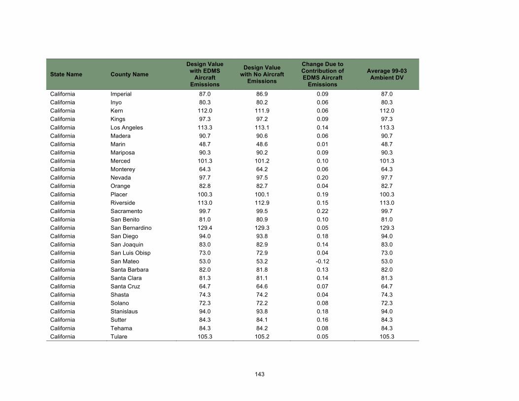
143



Aircraft Emissions


Emissions


Emissions


California Imperial 87.0 86.9 0.09 87.0 California Inyo 80.3 80.2 0.06 80.3 California Kern 112.0 111.9 0.06 112.0 California Kings 97.3 97.2 0.09 97.3 California Los Angeles 113.3 113.1 0.14 113.3 California Madera 90.7 90.6 0.06 90.7 California Marin 48.7 48.6 0.01 48.7 California Mariposa 90.3 90.2 0.09 90.3 California Merced 101.3 101.2 0.10 101.3 California Monterey 64.3 64.2 0.06 64.3 California Nevada 97.7 97.5 0.20 97.7 California Orange 82.8 82.7 0.04 82.7 California Placer 100.3 100.1 0.19 100.3 California Riverside 113.0 112.9 0.15 113.0 California Sacramento 99.7 99.5 0.22 99.7 California San Benito 81.0 80.9 0.10 81.0 California San Bernardino 129.4 129.3 0.05 129.3 California San Diego 94.0 93.8 0.18 94.0 California San Joaquin 83.0 82.9 0.14 83.0 California San Luis Obisp 73.0 72.9 0.04 73.0 California San Mateo 53.0 53.2 -0.12 53.0 California Santa Barbara 82.0 81.8 0.13 82.0 California Santa Clara 81.3 81.1 0.14 81.3 California Santa Cruz 64.7 64.6 0.07 64.7 California Shasta 74.3 74.2 0.04 74.3 California Solano 72.3 72.2 0.08 72.3 California Stanislaus 94.0 93.8 0.18 94.0 California Sutter 84.3 84.1 0.16 84.3 California Tehama 84.3 84.2 0.08 84.3 California Tulare 105.3 105.2 0.05 105.3

144



Aircraft Emissions


Emissions


Emissions


California Tuolumne 91.5 91.4 0.10 91.5 California Ventura 97.8 97.9 -0.09 97.7 California Yolo 82.7 82.6 0.13 82.7 Colorado Adams 65.0 65.2 -0.15 65.0 Colorado Arapahoe 77.7 77.7 0.00 77.7 Colorado Boulder 74.0 73.9 0.02 74.0 Colorado Denver 72.7 72.9 -0.16 72.7 Colorado Douglas 82.5 82.4 0.01 82.5 Colorado El Paso 71.0 70.9 0.02 71.0 Colorado Jefferson 83.7 83.6 0.02 83.7 Colorado La Plata 59.3 59.2 0.01 59.3 Colorado Larimer 77.7 77.6 0.01 77.7 Colorado Montezuma 68.3 68.2 0.01 68.3 Colorado Weld 74.3 74.2 0.03 74.3 Connecticut Fairfield 98.7 98.7 0.06 98.7 Connecticut Hartford 89.3 89.2 0.11 89.3 Connecticut Litchfield 83.0 82.9 0.06 83.0 Connecticut Middlesex 98.0 97.9 0.12 98.0 Connecticut New Haven 99.1 99.0 0.10 99.0 Connecticut New London 90.7 90.6 0.11 90.7 Connecticut Tolland 93.0 92.9 0.12 93.0 Delaware Kent 91.3 91.1 0.18 91.3 Delaware New Castle 95.3 95.2 0.11 95.3 Delaware Sussex 93.3 93.1 0.18 93.3 D.C. Washington 94.4 94.2 0.17 94.3 Florida Bay 79.9 79.9 0.06 80.0 Florida Duval 70.7 70.6 0.07 70.7 Florida Escambia 83.7 83.6 0.06 83.7 Florida Hillsborough 80.7 80.6 0.06 80.7 Florida Manatee 83.0 82.9 0.07 83.0

145



Aircraft Emissions


Emissions


Emissions


Florida Marion 75.7 75.6 0.03 75.7 Florida Orange 78.3 78.1 0.13 78.3 Florida Osceola 73.7 73.4 0.28 73.7 Florida Pasco 78.0 77.9 0.14 78.0 Florida Pinellas 78.3 78.2 0.06 78.3 Florida Polk 78.7 78.6 0.11 78.7 Florida Santa Rosa 82.0 81.9 0.04 82.0 Florida Sarasota 82.3 82.2 0.08 82.3 Florida Seminole 77.7 77.5 0.13 77.7 Florida Volusia 72.0 71.9 0.06 72.0 Florida Wakulla 76.0 75.9 0.11 76.0 Georgia Bibb 92.0 91.8 0.24 92.0 Georgia Chatham 71.0 70.9 0.07 71.0 Georgia Cherokee 77.0 76.9 0.13 77.0 Georgia Cobb 94.7 94.5 0.17 94.7 Georgia Coweta 92.0 91.7 0.32 92.0 Georgia Dawson 82.0 81.9 0.10 82.0 Georgia De Kalb 95.3 95.2 0.18 95.3 Georgia Douglas 94.8 94.4 0.39 94.7 Georgia Fayette 91.1 90.7 0.38 90.7 Georgia Fulton 99.4 99.0 0.41 99.0 Georgia Gwinnett 89.3 89.2 0.17 89.3 Georgia Henry 98.4 98.0 0.41 98.0 Georgia Murray 86.0 85.9 0.04 86.0 Georgia Muscogee 82.0 81.8 0.12 82.0 Georgia Paulding 90.3 90.2 0.09 90.3 Georgia Rockdale 96.5 95.9 0.60 96.3 Illinois Adams 76.0 75.9 0.04 76.0 Illinois Champaign 77.3 77.2 0.04 77.3 Illinois Clark 75.0 74.9 0.03 75.0

146



Aircraft Emissions


Emissions


Emissions


Illinois Cook 87.7 87.8 -0.07 87.7 Illinois Du Page 70.7 70.6 0.03 70.7 Illinois Effingham 77.7 77.6 0.06 77.7 Illinois Hamilton 78.7 78.6 0.03 78.7 Illinois Jersey 89.0 88.9 0.09 89.0 Illinois Kane 77.7 77.6 0.05 77.7 Illinois Lake 83.3 83.4 -0.15 83.3 Illinois McHenry 83.3 83.2 0.05 83.3 Illinois McLean 77.0 76.9 0.04 77.0 Illinois Macon 76.7 76.6 0.04 76.7 Illinois Macoupin 79.3 79.2 0.06 79.3 Illinois Madison 84.9 84.9 0.07 85.0 Illinois Peoria 79.0 78.9 0.05 79.0 Illinois Randolph 78.7 78.6 0.05 78.7 Illinois Rock Island 70.0 69.9 0.03 70.0 Illinois St Clair 83.2 83.2 0.06 83.3 Illinois Sangamon 76.0 75.9 0.05 76.0 Illinois Will 79.3 79.2 0.03 79.3 Illinois Winnebago 76.0 75.9 0.06 76.0 Indiana Allen 87.7 87.6 0.06 87.7 Indiana Boone 89.0 88.9 0.06 89.0 Indiana Carroll 84.0 83.9 0.05 84.0 Indiana Clark 89.4 89.3 0.10 89.3 Indiana Delaware 88.0 87.9 0.08 88.0 Indiana Floyd 83.7 83.6 0.08 83.7 Indiana Gibson 71.7 71.6 0.03 71.7 Indiana Greene 88.5 88.4 0.04 88.5 Indiana Hamilton 93.3 93.2 0.12 93.3 Indiana Hancock 91.7 91.6 0.08 91.7 Indiana Hendricks 86.5 86.4 0.10 86.5

147



Aircraft Emissions


Emissions


Emissions


Indiana Huntington 85.0 84.9 0.05 85.0 Indiana Jackson 85.0 84.9 0.07 85.0 Indiana Johnson 86.7 86.6 0.09 86.7 Indiana Lake 90.7 90.8 -0.07 90.7 Indiana La Porte 90.0 89.9 0.06 90.0 Indiana Madison 91.0 90.9 0.08 91.0 Indiana Marion 90.0 89.9 0.12 90.0 Indiana Morgan 86.7 86.6 0.10 86.7 Indiana Perry 90.0 89.9 0.07 90.0 Indiana Porter 89.0 89.0 0.04 89.0 Indiana Posey 85.7 85.6 0.04 85.7 Indiana St Joseph 89.0 88.9 0.09 89.0 Indiana Shelby 93.5 93.4 0.10 93.5 Indiana Vanderburgh 83.3 83.2 0.04 83.3 Indiana Vigo 87.0 86.9 0.03 87.0 Indiana Warrick 84.5 84.4 0.05 84.5 Iowa Bremer 70.5 70.4 0.02 70.5 Iowa Clinton 78.3 78.2 0.04 78.3 Iowa Harrison 75.6 75.6 0.06 75.7 Iowa Linn 71.0 70.9 0.03 71.0 Iowa Palo Alto 66.0 65.9 0.03 66.0 Iowa Polk 58.6 58.6 0.03 58.7 Iowa Scott 79.0 78.9 0.04 79.0 Iowa Story 63.2 63.2 0.03 63.3 Iowa Van Buren 73.7 73.6 0.03 73.7 Iowa Warren 63.3 63.2 0.02 63.3 Kansas Linn 76.7 76.6 0.03 76.7 Kansas Sedgwick 72.3 72.2 0.03 81.0 Kansas Wyandotte 80.3 80.3 0.02 80.3 Kentucky Bell 83.3 83.2 0.05 83.3

148



Aircraft Emissions


Emissions


Emissions


Kentucky Boone 85.3 85.2 0.07 85.3 Kentucky Boyd 88.3 88.2 0.04 88.3 Kentucky Bullitt 83.7 83.6 0.08 83.7 Kentucky Campbell 91.8 91.7 0.06 91.7 Kentucky Carter 80.3 80.2 0.03 80.3 Kentucky Christian 85.0 84.9 0.04 85.0 Kentucky Daviess 77.3 77.2 0.04 77.3 Kentucky Edmonson 84.0 83.9 0.05 84.0 Kentucky Fayette 78.3 78.2 0.05 78.3 Kentucky Graves 81.0 80.9 0.05 81.0 Kentucky Greenup 84.0 83.9 0.03 84.0 Kentucky Hancock 82.7 82.6 0.05 82.7 Kentucky Hardin 80.7 80.6 0.07 80.7 Kentucky Henderson 80.0 79.9 0.04 80.0 Kentucky Jefferson 84.4 84.3 0.10 84.3 Kentucky Jessamine 78.0 77.9 0.06 78.0 Kentucky Kenton 86.4 86.3 0.06 86.3 Kentucky Livingston 85.0 84.9 0.05 85.0 Kentucky McCracken 81.7 81.6 0.05 81.7 Kentucky McLean 84.0 83.9 0.04 84.0 Kentucky Oldham 88.1 88.0 0.10 88.0 Kentucky Perry 74.7 74.6 0.03 74.7 Kentucky Pike 76.3 76.2 0.03 76.3 Kentucky Pulaski 81.3 81.2 0.05 81.3 Kentucky Scott 70.7 70.6 0.07 70.7 Kentucky Simpson 84.0 83.9 0.04 84.0 Kentucky Trigg 76.7 76.6 0.05 76.7 Kentucky Warren 84.0 83.9 0.05 84.0 Louisiana Ascension 81.7 81.6 0.03 81.7 Louisiana Beauregard 75.0 74.9 0.02 75.0

149



Aircraft Emissions


Emissions


Emissions


Louisiana Bossier 84.7 84.6 0.05 84.7 Louisiana Caddo 79.7 79.6 0.05 79.7 Louisiana Calcasieu 81.7 81.6 0.02 81.7 Louisiana East Baton Rou 87.3 87.2 0.03 87.3 Louisiana Iberville 86.7 86.6 0.03 86.7 Louisiana Jefferson 85.3 85.3 0.02 85.3 Louisiana Lafayette 80.7 80.6 0.03 80.7 Louisiana Lafourche 81.0 80.9 0.04 81.0 Louisiana Livingston 83.3 83.2 0.03 83.3 Louisiana Orleans 72.0 72.0 0.02 72.0 Louisiana Ouachita 78.7 78.6 0.05 78.7 Louisiana Pointe Coupee 73.0 72.9 0.03 73.0 Louisiana St Bernard 79.3 79.3 0.02 79.3 Louisiana St Charles 81.7 81.6 0.03 81.7 Louisiana St James 77.3 77.2 0.04 77.3 Louisiana St John The Ba 81.7 81.6 0.03 81.7 Louisiana St Mary 78.0 77.9 0.03 78.0 Louisiana West Baton Rou 85.7 85.6 0.04 85.7 Maine Cumberland 84.7 84.6 0.10 84.7 Maine Hancock 92.0 91.8 0.16 92.0 Maine Kennebec 77.7 77.6 0.11 77.7 Maine Knox 83.3 83.2 0.14 83.3 Maine Oxford 61.0 60.9 0.03 61.0 Maine Penobscot 83.0 82.9 0.12 83.0 Maine Piscataquis 65.0 64.9 0.03 65.0 Maine York 89.0 88.9 0.08 89.0 Maryland Anne Arundel 101.1 100.8 0.23 101.0 Maryland Baltimore 93.0 92.9 0.14 93.0 Maryland Calvert 89.0 88.8 0.26 89.0 Maryland Carroll 91.3 91.2 0.15 91.3

150



Aircraft Emissions


Emissions


Emissions


Maryland Cecil 102.7 102.6 0.12 102.7 Maryland Charles 94.7 94.5 0.18 94.7 Maryland Frederick 90.0 89.9 0.15 90.0 Maryland Harford 103.7 103.5 0.16 103.7 Maryland Kent 99.0 98.8 0.14 99.0 Maryland Montgomery 88.7 88.6 0.10 88.7 Maryland Prince Georges 95.0 94.9 0.11 95.0 Maryland Washington 86.0 85.9 0.07 86.0 Massachusetts Barnstable 94.7 94.6 0.10 94.7 Massachusetts Berkshire 87.0 86.9 0.05 87.0 Massachusetts Bristol 92.7 92.6 0.12 92.7 Massachusetts Essex 89.7 89.6 0.07 89.7 Massachusetts Hampden 90.3 90.2 0.08 90.3 Massachusetts Hampshire 88.3 88.2 0.08 88.3 Massachusetts Middlesex 88.7 88.6 0.09 88.7 Massachusetts Suffolk 88.1 88.1 -0.02 88.0 Massachusetts Worcester 85.3 85.2 0.10 85.3 Michigan Allegan 92.0 91.9 0.11 92.0 Michigan Benzie 87.7 87.6 0.13 87.7 Michigan Berrien 88.3 88.2 0.09 88.3 Michigan Cass 90.0 89.9 0.06 90.0 Michigan Clinton 83.3 83.2 0.09 83.3 Michigan Genesee 86.7 86.6 0.11 86.7 Michigan Huron 84.0 83.9 0.05 84.0 Michigan Ingham 83.3 83.2 0.09 83.3 Michigan Kalamazoo 83.0 82.9 0.06 83.0 Michigan Kent 84.7 84.6 0.09 84.7 Michigan Lenawee 85.0 84.9 0.08 85.0 Michigan Macomb 91.0 90.9 0.08 91.0 Michigan Mason 89.0 88.9 0.13 89.0

151



Aircraft Emissions


Emissions


Emissions


Michigan Missaukee 80.3 80.2 0.06 80.3 Michigan Muskegon 92.0 91.9 0.10 92.0 Michigan Oakland 87.0 86.9 0.08 87.0 Michigan Ottawa 86.0 85.9 0.07 86.0 Michigan St Clair 87.7 87.6 0.09 87.7 Michigan Washtenaw 88.4 88.4 0.00 88.3 Michigan Wayne 88.0 87.9 0.08 88.0 Minnesota Anoka 71.0 71.1 -0.12 71.0 Minnesota Washington 75.0 74.9 0.10 75.0 Mississippi Adams 79.7 79.6 0.05 79.7 Mississippi Bolivar 78.0 77.9 0.05 78.0 Mississippi De Soto 84.4 84.2 0.22 84.3 Mississippi Hancock 83.7 83.6 0.01 83.7 Mississippi Harrison 83.3 83.2 0.04 83.3 Mississippi Hinds 76.3 76.2 0.08 76.3 Mississippi Jackson 83.0 82.9 0.03 83.0 Mississippi Madison 76.3 76.2 0.08 76.3 Mississippi Warren 76.7 76.6 0.04 76.7 Missouri Cass 79.0 78.9 0.03 79.0 Missouri Clay 84.3 84.2 0.03 84.3 Missouri Jefferson 87.2 87.2 0.08 87.3 Missouri Monroe 79.2 79.2 0.04 79.3 Missouri Platte 81.7 81.7 0.02 81.7 Missouri St Charles 90.7 90.6 0.09 90.7 Missouri Ste Genevieve 83.9 83.9 0.05 84.0 Missouri St Louis 89.4 89.3 0.09 89.3 Missouri St Louis City 86.9 86.9 0.06 87.0 Nebraska Douglas 67.5 67.4 0.03 67.5 Nevada Clark 84.5 84.2 0.31 84.5 Nevada Douglas 71.7 71.6 0.06 71.7

152



Aircraft Emissions


Emissions


Emissions


Nevada Washoe 73.3 73.2 0.05 73.3 Nevada White Pine 72.0 71.9 0.02 72.0 Nevada Carson City 68.7 68.6 0.05 68.7 New Hampshire Belknap 78.0 77.9 0.05 78.0 New Hampshire Carroll 66.5 66.4 0.03 66.5 New Hampshire Cheshire 73.7 73.6 0.03 73.7 New Hampshire Grafton 69.7 69.6 0.02 69.7 New Hampshire Hillsborough 85.0 84.9 0.06 85.0 New Hampshire Merrimack 73.0 72.9 0.08 73.0 New Hampshire Rockingham 82.7 82.6 0.09 82.7 New Hampshire Strafford 77.3 77.2 0.05 77.3 New Hampshire Sullivan 73.3 73.2 0.03 73.3 New Jersey Atlantic 90.3 90.2 0.12 90.3 New Jersey Bergen 92.5 92.5 -0.02 92.5 New Jersey Camden 102.3 102.2 0.14 102.3 New Jersey Cumberland 96.7 96.5 0.16 96.7 New Jersey Essex 67.0 67.2 -0.19 67.0 New Jersey Gloucester 100.4 100.4 -0.06 100.3 New Jersey Hudson 88.0 88.3 -0.25 88.0 New Jersey Hunterdon 97.3 97.2 0.09 97.3 New Jersey Mercer 102.3 102.2 0.10 102.3 New Jersey Middlesex 100.7 100.6 0.11 100.7 New Jersey Monmouth 95.7 95.7 -0.01 95.7 New Jersey Morris 97.7 97.6 0.06 97.7 New Jersey Ocean 109.0 108.9 0.12 109.0 New Jersey Passaic 88.3 88.3 -0.02 88.3 New Mexico Bernalillo 75.7 75.6 0.03 75.7 New Mexico Dona Ana 79.7 79.6 0.02 79.7 New Mexico Eddy 69.0 68.9 0.02 69.0 New Mexico Sandoval 72.0 71.9 0.02 72.0

153



Aircraft Emissions


Emissions


Emissions


New Mexico San Juan 75.0 74.9 0.02 75.0 New Mexico Valencia 68.0 67.9 0.03 68.0 New York Albany 83.0 82.9 0.05 83.0 New York Bronx 82.8 82.9 -0.14 82.7 New York Chautauqua 91.7 91.6 0.06 91.7 New York Chemung 81.0 80.9 0.04 81.0 New York Dutchess 91.3 91.2 0.05 91.3 New York Erie 96.0 95.9 0.06 96.0 New York Essex 89.0 88.9 0.06 89.0 New York Hamilton 79.0 78.9 0.04 79.0 New York Herkimer 74.0 73.9 0.05 74.0 New York Jefferson 91.7 91.6 0.07 91.7 New York Madison 80.0 79.9 0.05 80.0 New York Monroe 86.5 86.4 0.06 86.5 New York Niagara 91.0 90.9 0.07 91.0 New York Oneida 79.0 78.9 0.05 79.0 New York Onondaga 83.0 82.9 0.05 83.0 New York Orange 86.0 85.9 0.07 86.0 New York Putnam 91.3 91.2 0.09 91.3 New York Queens 85.1 85.3 -0.14 85.0 New York Richmond 96.0 96.3 -0.27 96.0 New York Saratoga 85.5 85.4 0.06 85.5 New York Schenectady 77.3 77.2 0.05 77.3 New York Suffolk 98.5 98.5 0.07 98.5 New York Ulster 81.7 81.6 0.06 81.7 New York Wayne 84.0 83.9 0.06 84.0 New York Westchester 92.0 92.0 0.04 92.0 North Carolina Alexander 88.7 88.6 0.07 88.7 North Carolina Avery 78.3 78.2 0.04 78.3 North Carolina Buncombe 82.0 81.9 0.05 82.0

154



Aircraft Emissions


Emissions


Emissions


North Carolina Caldwell 85.7 85.6 0.06 85.7 North Carolina Camden 80.0 79.9 0.09 80.0 North Carolina Caswell 89.7 89.6 0.06 89.7 North Carolina Chatham 82.0 81.9 0.07 82.0 North Carolina Cumberland 87.7 87.6 0.09 87.7 North Carolina Davie 94.7 94.6 0.09 94.7 North Carolina Durham 89.0 88.9 0.04 89.0 North Carolina Edgecombe 88.0 87.9 0.08 88.0 North Carolina Forsyth 93.7 93.6 0.07 93.7 North Carolina Franklin 89.0 88.9 0.09 89.0 North Carolina Granville 92.0 91.9 0.05 92.0 North Carolina Guilford 90.7 90.6 0.05 90.7 North Carolina Haywood 86.3 86.2 0.05 86.3 North Carolina Jackson 85.5 85.4 0.03 85.5 North Carolina Johnston 85.6 85.5 0.14 85.7 North Carolina Lincoln 92.3 92.2 0.05 92.3 North Carolina Mecklenburg 100.3 100.2 0.12 100.3 North Carolina New Hanover 77.3 77.2 0.09 77.3 North Carolina Northampton 83.3 83.2 0.05 83.3 North Carolina Person 90.0 89.9 0.05 90.0 North Carolina Randolph 85.0 84.9 0.10 85.0 North Carolina Rockingham 88.7 88.6 0.05 88.7 North Carolina Rowan 99.7 99.6 0.12 99.7 North Carolina Swain 73.7 73.6 0.04 73.7 North Carolina Union 87.7 87.5 0.23 87.7 North Carolina Wake 92.7 92.5 0.23 92.7 North Carolina Yancey 86.3 86.2 0.04 86.3 Ohio Allen 87.7 87.6 0.04 87.7 Ohio Ashtabula 94.0 93.9 0.08 94.0 Ohio Butler 89.0 88.9 0.09 89.0

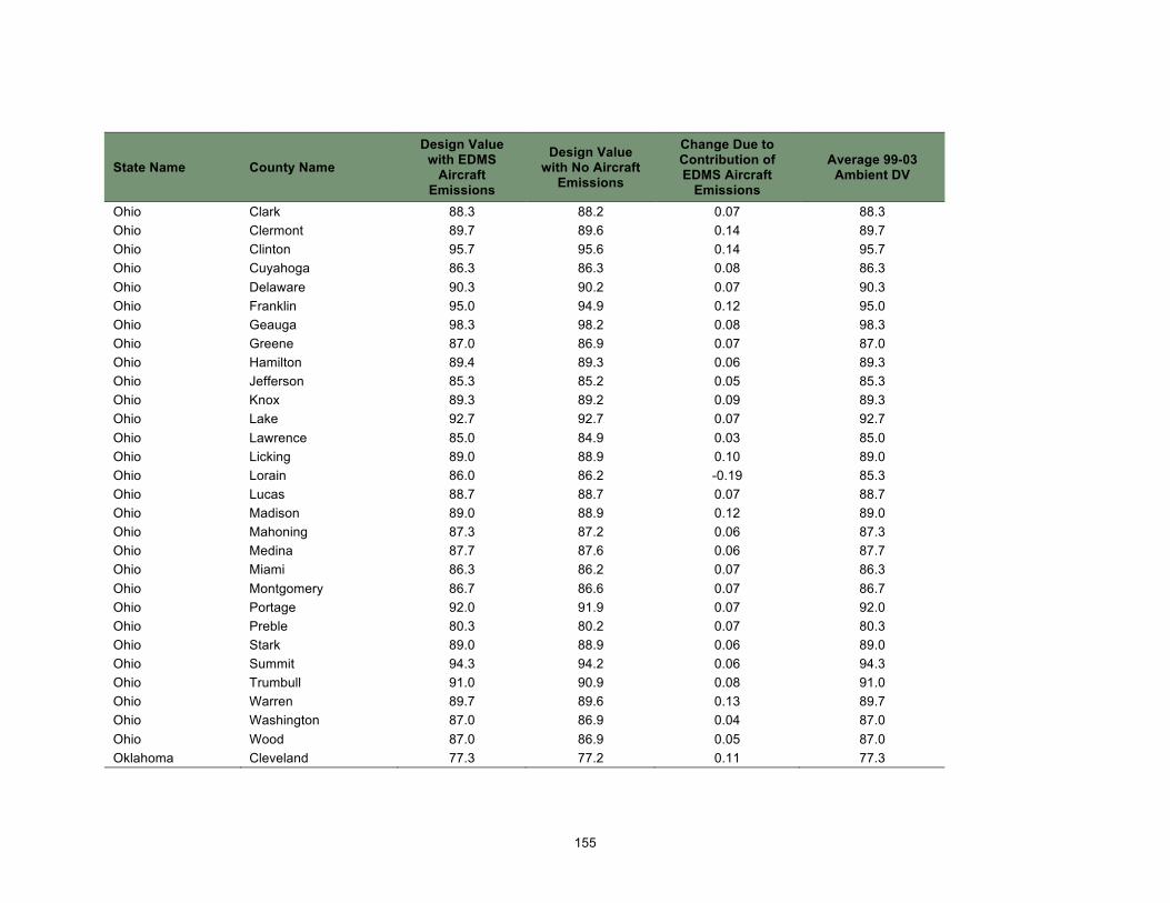
155



Aircraft Emissions


Emissions


Emissions


Ohio Clark 88.3 88.2 0.07 88.3 Ohio Clermont 89.7 89.6 0.14 89.7 Ohio Clinton 95.7 95.6 0.14 95.7 Ohio Cuyahoga 86.3 86.3 0.08 86.3 Ohio Delaware 90.3 90.2 0.07 90.3 Ohio Franklin 95.0 94.9 0.12 95.0 Ohio Geauga 98.3 98.2 0.08 98.3 Ohio Greene 87.0 86.9 0.07 87.0 Ohio Hamilton 89.4 89.3 0.06 89.3 Ohio Jefferson 85.3 85.2 0.05 85.3 Ohio Knox 89.3 89.2 0.09 89.3 Ohio Lake 92.7 92.7 0.07 92.7 Ohio Lawrence 85.0 84.9 0.03 85.0 Ohio Licking 89.0 88.9 0.10 89.0 Ohio Lorain 86.0 86.2 -0.19 85.3 Ohio Lucas 88.7 88.7 0.07 88.7 Ohio Madison 89.0 88.9 0.12 89.0 Ohio Mahoning 87.3 87.2 0.06 87.3 Ohio Medina 87.7 87.6 0.06 87.7 Ohio Miami 86.3 86.2 0.07 86.3 Ohio Montgomery 86.7 86.6 0.07 86.7 Ohio Portage 92.0 91.9 0.07 92.0 Ohio Preble 80.3 80.2 0.07 80.3 Ohio Stark 89.0 88.9 0.06 89.0 Ohio Summit 94.3 94.2 0.06 94.3 Ohio Trumbull 91.0 90.9 0.08 91.0 Ohio Warren 89.7 89.6 0.13 89.7 Ohio Washington 87.0 86.9 0.04 87.0 Ohio Wood 87.0 86.9 0.05 87.0 Oklahoma Cleveland 77.3 77.2 0.11 77.3

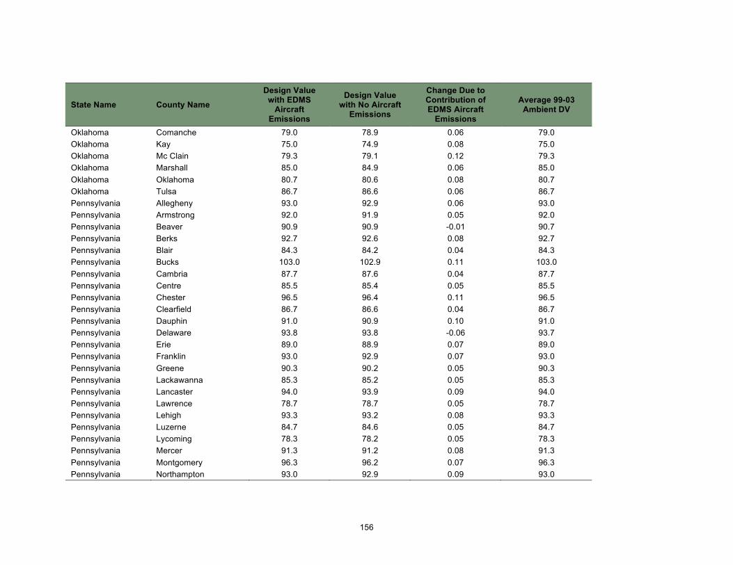
156



Aircraft Emissions


Emissions


Emissions


Oklahoma Comanche 79.0 78.9 0.06 79.0 Oklahoma Kay 75.0 74.9 0.08 75.0 Oklahoma Mc Clain 79.3 79.1 0.12 79.3 Oklahoma Marshall 85.0 84.9 0.06 85.0 Oklahoma Oklahoma 80.7 80.6 0.08 80.7 Oklahoma Tulsa 86.7 86.6 0.06 86.7 Pennsylvania Allegheny 93.0 92.9 0.06 93.0 Pennsylvania Armstrong 92.0 91.9 0.05 92.0 Pennsylvania Beaver 90.9 90.9 -0.01 90.7 Pennsylvania Berks 92.7 92.6 0.08 92.7 Pennsylvania Blair 84.3 84.2 0.04 84.3 Pennsylvania Bucks 103.0 102.9 0.11 103.0 Pennsylvania Cambria 87.7 87.6 0.04 87.7 Pennsylvania Centre 85.5 85.4 0.05 85.5 Pennsylvania Chester 96.5 96.4 0.11 96.5 Pennsylvania Clearfield 86.7 86.6 0.04 86.7 Pennsylvania Dauphin 91.0 90.9 0.10 91.0 Pennsylvania Delaware 93.8 93.8 -0.06 93.7 Pennsylvania Erie 89.0 88.9 0.07 89.0 Pennsylvania Franklin 93.0 92.9 0.07 93.0 Pennsylvania Greene 90.3 90.2 0.05 90.3 Pennsylvania Lackawanna 85.3 85.2 0.05 85.3 Pennsylvania Lancaster 94.0 93.9 0.09 94.0 Pennsylvania Lawrence 78.7 78.7 0.05 78.7 Pennsylvania Lehigh 93.3 93.2 0.08 93.3 Pennsylvania Luzerne 84.7 84.6 0.05 84.7 Pennsylvania Lycoming 78.3 78.2 0.05 78.3 Pennsylvania Mercer 91.3 91.2 0.08 91.3 Pennsylvania Montgomery 96.3 96.2 0.07 96.3 Pennsylvania Northampton 93.0 92.9 0.09 93.0

157



Aircraft Emissions


Emissions


Emissions


Pennsylvania Perry 84.7 84.6 0.05 84.7 Pennsylvania Philadelphia 97.5 97.4 0.10 97.5 Pennsylvania Tioga 83.7 83.6 0.04 83.7 Pennsylvania Washington 87.7 87.6 0.05 87.7 Pennsylvania Westmoreland 87.7 87.6 0.05 87.7 Pennsylvania York 90.3 90.2 0.09 90.3 Rhode Island Kent 95.3 95.2 0.15 95.3 Rhode Island Providence 90.3 90.2 0.17 90.3 Rhode Island Washington 93.3 93.1 0.14 93.3 South Carolina Abbeville 84.0 83.8 0.18 84.0 South Carolina Anderson 88.0 87.9 0.08 88.0 South Carolina Berkeley 74.0 73.9 0.10 74.0 South Carolina Charleston 72.0 71.9 0.06 72.0 South Carolina Cherokee 86.0 85.9 0.11 86.0 South Carolina Chester 84.3 84.1 0.17 84.3 South Carolina Darlington 84.7 84.6 0.07 84.7 South Carolina Edgefield 80.7 80.6 0.07 80.7 South Carolina Oconee 84.5 84.4 0.04 84.5 South Carolina Pickens 85.3 85.2 0.06 85.3 South Carolina Richland 91.7 91.6 0.11 91.7 South Carolina Spartanburg 90.0 89.9 0.10 90.0 South Carolina Union 80.7 80.6 0.12 80.7 South Carolina York 83.3 83.1 0.17 83.3 Tennessee Anderson 89.7 89.6 0.05 89.7 Tennessee Blount 94.0 93.9 0.07 94.0 Tennessee Davidson 81.3 81.2 0.12 81.3 Tennessee Hamilton 90.7 90.6 0.08 90.7 Tennessee Haywood 85.3 85.2 0.13 85.3 Tennessee Jefferson 94.0 93.9 0.06 94.0 Tennessee Knox 94.7 94.6 0.08 94.7

158



Aircraft Emissions


Emissions


Emissions


Tennessee Lawrence 79.3 79.2 0.04 79.3 Tennessee Meigs 90.5 90.4 0.06 90.5 Tennessee Putnam 85.0 84.9 0.05 85.0 Tennessee Rutherford 83.3 83.2 0.10 83.3 Tennessee Sevier 96.0 95.9 0.05 96.0 Tennessee Shelby 90.9 90.5 0.38 90.7 Tennessee Sullivan 89.3 89.2 0.07 89.3 Tennessee Sumner 89.0 88.9 0.09 89.0 Tennessee Williamson 86.3 86.2 0.07 86.3 Tennessee Wilson 84.7 84.6 0.09 84.7 Texas Bexar 85.7 85.6 0.06 85.7 Texas Brazoria 91.0 90.9 0.11 91.0 Texas Collin 93.3 93.3 0.00 93.3 Texas Dallas 91.0 90.9 0.08 91.0 Texas Denton 99.0 98.6 0.45 99.0 Texas Ellis 85.3 85.2 0.09 85.3 Texas El Paso 78.7 78.6 0.04 78.7 Texas Galveston 92.0 91.9 0.05 92.0 Texas Gregg 88.3 88.2 0.03 88.3 Texas Harris 105.1 105.0 0.13 105.0 Texas Harrison 76.0 75.9 0.04 76.0 Texas Hood 84.0 83.8 0.16 84.0 Texas Jefferson 90.5 90.4 0.03 90.5 Texas Johnson 89.5 89.3 0.15 89.5 Texas Marion 81.0 80.9 0.04 81.0 Texas Montgomery 90.7 90.5 0.22 90.7 Texas Orange 78.3 78.2 0.03 78.3 Texas Parker 87.5 87.2 0.30 87.5 Texas Rockwall 82.0 81.9 0.06 82.0 Texas Smith 84.3 84.2 0.03 84.3

159



Aircraft Emissions


Emissions


Emissions


Texas Tarrant 98.4 98.1 0.35 98.3 Texas Travis 84.2 84.2 0.07 84.3 Utah Box Elder 79.0 78.9 0.08 79.0 Utah Cache 69.3 69.2 0.03 69.3 Utah Davis 81.3 81.3 0.05 81.3 Utah Salt Lake 80.0 80.0 0.04 80.0 Utah San Juan 71.0 70.9 0.01 71.0 Utah Utah 78.3 78.2 0.01 78.3 Utah Weber 77.7 77.6 0.10 77.7 Vermont Bennington 79.7 79.6 0.06 79.7 Vermont Chittenden 76.7 76.6 0.04 76.7 Virginia Arlington 95.8 95.6 0.17 95.7 Virginia Caroline 84.0 83.9 0.13 84.0 Virginia Charles City 89.3 89.2 0.08 89.3 Virginia Chesterfield 86.0 85.9 0.07 86.0 Virginia Fairfax 96.4 96.2 0.17 96.3 Virginia Fauquier 81.0 80.9 0.12 81.0 Virginia Frederick 84.3 84.2 0.04 84.3 Virginia Hanover 94.0 93.9 0.08 94.0 Virginia Henrico 90.0 89.9 0.08 90.0 Virginia Loudoun 89.5 89.1 0.35 89.3 Virginia Madison 86.3 86.2 0.09 86.3 Virginia Page 81.3 81.2 0.09 81.3 Virginia Prince William 85.7 85.6 0.15 85.7 Virginia Roanoke 86.0 85.9 0.07 86.0 Virginia Rockbridge 79.0 78.9 0.04 79.0 Virginia Stafford 86.4 86.1 0.27 86.3 Virginia Wythe 80.7 80.6 0.04 80.7 Virginia Alexandria Cit 90.1 89.9 0.16 90.0 Virginia Hampton City 88.7 88.6 0.09 88.7

160



Aircraft Emissions


Emissions


Emissions


Virginia Suffolk City 87.3 87.2 0.09 87.3 West Virginia Berkeley 86.0 85.9 0.04 86.0 West Virginia Cabell 88.0 87.9 0.04 88.0 West Virginia Greenbrier 81.7 81.6 0.04 81.7 West Virginia Hancock 84.3 84.2 0.05 84.3 West Virginia Kanawha 87.0 86.9 0.05 87.0 West Virginia Monongalia 80.0 79.9 0.04 80.0 West Virginia Ohio 84.7 84.6 0.05 84.7 West Virginia Wood 87.7 87.6 0.04 87.7 Wisconsin Brown 81.7 81.6 0.09 81.7 Wisconsin Columbia 77.7 77.6 0.07 77.7 Wisconsin Dane 77.3 77.2 0.07 77.3 Wisconsin Dodge 81.0 80.9 0.07 81.0 Wisconsin Door 92.7 92.6 0.12 92.7 Wisconsin Fond Du Lac 79.0 78.9 0.11 79.0 Wisconsin Green 74.5 74.4 0.05 74.5 Wisconsin Jefferson 84.5 84.4 0.09 84.5 Wisconsin Kenosha 98.7 98.9 -0.18 98.7 Wisconsin Kewaunee 90.0 89.9 0.13 90.0 Wisconsin Manitowoc 90.0 89.9 0.12 90.0 Wisconsin Milwaukee 91.6 91.7 -0.07 91.3 Wisconsin Outagamie 77.3 77.2 0.06 77.3 Wisconsin Ozaukee 95.4 95.4 0.01 95.3 Wisconsin Racine 91.7 91.7 -0.06 91.7 Wisconsin Rock 84.3 84.2 0.11 84.3 Wisconsin St Croix 72.7 72.6 0.12 72.7 Wisconsin Sauk 74.3 74.2 0.05 74.3 Wisconsin Sheboygan 98.0 97.9 0.10 98.0 Wisconsin Walworth 83.3 83.2 0.11 83.3 Wisconsin Washington 82.7 82.6 0.13 82.7

161



Aircraft Emissions


Emissions


Emissions


Wisconsin Waukesha 82.7 82.6 0.12 82.7 Wisconsin Winnebago 80.0 79.9 0.08 80.0 Wyoming Campbell 71.0 70.9 0.01 71.0 Wyoming Teton 65.7 65.6 0.01 65.7

162

Appendix G Health Impact Functions and Baseline Incidence Rates

Health impact functions relate the change in the number of observed health events for a population to a change in ambient concentration of a particular air pollutant. A standard health impact function has four components: 1) an effect estimate for a particular study; 2) a baseline incidence rate for the health effect (obtained from epidemiological literature or a source of public health statistics); 3) the size of the potentially affected population; 4) the estimated change in the relevant pollutant summary measure (for example, a change in ambient ozone or PM concentrations). Generally health impact functions are assumed to have a log-linear form:

∆y = y0 · (eß·∆P – 1)

Where: y0 is the baseline incidence rate (number of incidences in a specific subpopulation) ß is the effect estimate provided by the study ∆y is the change in health incidences ∆P is the change in the summary measure of the pollutant being examined

The EPA Benefits Modeling and Analysis Program (BenMAP) incorporates the elements necessary to conduct a nationwide analysis by combining air pollution monitor data, air quality modeling data, census data, and population projections to calculate a population’s potential exposure to ambient air pollution. This Appendix contains the health impact functions and incidence rates used in BenMAP.

163

Table G.1: Health impact functions used in BenMAP to estimate benefits of PM reductions

Health Endpoint Study Population Used in BenMAP

Premature mortality (Pope et al., 2002) (function based on average of PM2.5 measures)

>29 years

(Woodruff et al., 1997) Infant (<1 year)

Chronic Illness

Chronic Bronchitis (Abbey et al., 1995) >26 years

Myocardial Infarctions, Nonfatal (Peters et al., 2001) >17 years

Hospital Admissions

Respiratory (Moolgavkar, 2003) (COPD) >64 years

(Ito, 2003) (COPD) >64 years

(Moolgavkar, 2000a) (COPD, less Asthma)

18-64 years

(Ito, 2003) (Pneumonia) >64 years

(Sheppard, 2003) (Asthma) <65 years

Cardiovascular (Moolgavkar, 2000b) (All Cardiovascular, less MI)

18-64 years

(Moolgavkar, 2003) (All Cardiovascular, less MI)

>64 years

(Ito, 2003) (Ischemic Heart Disease, less MI; Dysrhythmia; Heart Failure)

>64 years

ER Visits, Asthma (Norris et al., 1999) <18 years

Other Health Endpoints

Acute Bronchitis (Dockery et al., 1996) 8-12 years

Upper Respiratory Symptoms (Pope et al., 1991) 9-11 years

Lower Respiratory Symptoms (Schwartz and Neas, 2000) 7-14 years

Asthma Exacerbation

164


(Ostro et al., 2001) (Wheeze, Cough, Shortness of Breath)

6-18 years

(Vedal et al., 1998) (Cough) 6-18 years

Work Loss Days (Ostro, 1987) 18-64 years

Minor Restricted Activity Days (Ostro and Rothschild, 1989) 18-64 years

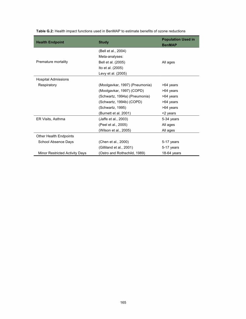
165

Table G.2: Health impact functions used in BenMAP to estimate benefits of ozone reductions


Premature mortality

(Bell et al., 2004) Meta-analyses: Bell et al. (2005) Ito et al. (2005) Levy et al. (2005)

All ages

Hospital Admissions Respiratory (Moolgavkar, 1997) (Pneumonia) >64 years (Moolgavkar, 1997) (COPD) >64 years (Schwartz, 1994a) (Pneumonia) >64 years (Schwartz, 1994b) (COPD) >64 years (Schwartz, 1995) >64 years (Burnett et al. 2001) <2 years ER Visits, Asthma (Jaffe et al., 2003) 5-34 years (Peel et al., 2005) All ages (Wilson et al., 2005) All ages Other Health Endpoints School Absence Days (Chen et al., 2000) 5-17 years (Gilliland et al., 2001) 5-17 years Minor Restricted Activity Days (Ostro and Rothschild, 1989) 18-64 years

166

Table G.3: Baseline incidence rates used in BenMAP for the general population

Endpoint Parameter Incidence Value Source

Mortality Daily or annual mortality rate

Age-, cause-, and county-specific rate

CDC Wonder (1996-1998)

Hospitalizations Daily hospitalization rate Age-, region-, and cause-specific rate

1999 National Hospital Discharge Survey (NHDS) public use data files141

Asthma ER Visits Daily Asthma ER Visit Rate

Age- and Region-Specific

2000 National Hospital Ambulatory Medical Care Survey (NHAMCS)142, 1999 National Hospital Discharge Survey (NHDS)143

Annual Prevalence Rate per person by age

18-44: 0.0367 45-64: 0.0505 65+: 0.0587

1999 National Health Interview Survey (NHIS) (American Lung Association, 2002b)

Chronic Bronchitis

Annual Incidence Rate per person

0.00378 (Abbey et al., 1993)

Nonfatal Myocardial Infarction

Daily rates per person 18+ by region

Northeast: 0.0000159 Midwest: 0.0000135 South: 0.0000111 West: 0.0000100

1999 NHDS public use data files, adjusted by 0.93 for probability of surviving after 28 (Rosamond et al., 1999)

Incidence (and Prevalence) among asthmatic African-American children

Daily Wheeze: 0.076 (0.173) Daily Cough: 0.067 (0.145) Daily shortness of breath: 0.037 (0.074)

(Ostro et al., 2001)

Asthma Exacerbations

Prevalence among asthmatic children

Daily Wheeze: 0.038 Daily Cough: 0.086 Daily shortness of breath: 0.045

(Vedal et al., 1998)

Acute Bronchitis Annual Rate144, Children 0.043 (American Lung Association, 2002c)

Lower Respiratory Symptoms

Daily Rate, Children 0.0012 (Schwartz et al., 1994)

Upper Respiratory Symptoms

Daily Rate, Asthmatic Children

0.3419 (Pope et al., 1991)

141 See ftp://ftp.cdc.gov/pub/Health_Statistics/NCHS/Datasets/NHDS 142 See ftp://ftp.cdc.gov/pub/Health_Statistics/NCHS/Datasets/NHAMCS 143 See ftp://ftp.cdc.gov/pub/Health_Statistics/NCHS/Datasets/NHDS 144 Defined as two or more of the following: cough, chest pain, phlegm, or wheeze

167

Endpoint Parameter Incidence Value Source

Work Loss Days Daily Rate, by Age 18-24: 0.00540 25-44: 0.00678 45-64: 0.00492

1996 National Health Interview Survey (HIS) (Adams, Hendershot, & Marano, 1999); U.S. Bureau of the Census

Minor Restricted Activity Days

Daily Rate per person 0.02137 (Ostro & Rothschild, 1989)

Table G.4: Asthma prevalence rates used in BenMAP

Population Group Value Source All Ages 0.0386 (American Lung Association, 2002a) <18 0.0527 (American Lung Association, 2002a) 5-17 0.0567 (American Lung Association, 2002a) 18-44 0.0371 (American Lung Association, 2002a) 45-64 0.0333 (American Lung Association, 2002a) 65+ 0.0221 (American Lung Association, 2002a) Male, 27+ 0.021 2000 NHIS Public Use Data Files145 African American, 5 to 17 0.0726 (American Lung Association, 2002a) African American <18 0.0735 (American Lung Association, 2002a)

Studies Referenced:

Abbey, D. E., Colome, S. D., Mills, P. K., Burchette, R., Beeson, W. L., & Tian, Y. (1993). Chronic Disease Associated with Long-Term Concentration of Nitrogen Dioxide. Journal of Exposure Analysis and Environmental Epidemiology, 3(2), 181-202.

Abbey, D. E., B. E. Ostro, et al. (1995). "Chronic Respiratory Symptoms Associated with Estimated Long-Term Ambient Concentrations of Fine Particulates Less Than 2.5 Microns in Aerodynamic Diameter (PM2.5) and Other Air Pollutants." J Expo Anal Environ Epidemiol 5(2): 137-159.

Adams, P. F., Hendershot, G. E., & Marano, M. A. (1999). Current Estimates from the National Health Interview Survey, 1996. Vital Health Statistics, 10(200), 1-212.

American Lung Association. 2002a. Trends in Asthma Morbidity and Mortality. American Lung Association, Best Practices and Program Services, Epidemiology and Statistics Unit.

American Lung Association. 2002b. Trends in Chronic Bronchitis and Emphysema: Morbidity and Mortality. Amperican Lung Association, Best Practices and Program Services, Epidemiology and Statistics Unit.

American Lung Association. 2002c. Trends in Morbidity and Mortality: Pneumonia, Influenza, and Acute Respiratory Conditions. American Lung Association, Best Practices and Program Services, Epidemiology and Statistics Unit.

Bell, M. L., McDermott, A., Zeger, S. L., Samet, J. M., Dominici, F. (2004). Ozone and short-term mortality in 95 US urban communities, 1987-2000. Journal of the American Medical Association, 292(19): p. 2372-8.

145 See ftp://ftp.cdc.gov/pub/Health_Statistics/NCHS/Datasets/NHIS/2000/

168

Bell, M. L., Dominici, F., Samet, J. M. (2005). A meta-analysis of time-series studies of ozone and mortality with comparison to the national morbidity, mortality, and air pollution study. Epidemiology. 16(4): p. 436-45.

Burnett, R. T., Smith-Doiron, M., Stieb, D., Raizenne, M. E., Brook, J. R., Dales, R. E., Leech, J. A., Cakmak, S., & Krewski, D. (2001). Association between Ozone and Hospitalization for Acute Respiratory Disease in Children less than 2 Years of Age. American Journal of Epidemiology, 153, 444-452.

Chen, L., Jennison, B. L., Yang, W., & Omaye, S. T. (2000). Elementary School Absenteeism and Air Pollution. Inhalation Toxicology, 12(11), 997-1016.

Cocker, T. D., & Horst, R. L. J. (1981). Hours of Work, Labor Productivity, and Environmental Conditions: A Case Study. The Review of Economics and Statistics, 63, 361-368.

Dockery, D. W., J. Cunningham, et al. (1996). "Health Effects of Acid Aerosols on North American Children - Respiratory Symptoms." Environmental Health Perspectives 104(5): 500-505.

Gilliland, F. D., Berhane, K., Rappaport, E. B., Thomas, D. C., Avol, E., Gauderman, W. J., London, S. J., Margolis, H. G., McConnell, R., Islam, K. T., & Peters, J. M. (2001). The Effects of Ambient Air Pollution on School Absenteeism due to Respiratory Illness. Epidemiology, 12(1), 43-54.

Ito, K. (2003). Associations of Particulate Matter Components with Daily Mortality and Morbidity in Detroit, Michigan. In: Revised Analyses of Time-Series Studies of Air Pollution and Health. Boston, MA, Health Effects Institute: 143-156.

Ito, K., De Leon, S. F., & Lippmann, M. (2005). Associations between Ozone and Daily Mortality: Analysis and Meta-Analysis. Epidemiology, 16(4), 446-457.

Jaffe, D., Singer, M., & Rimm, A. (2003). Air Pollution and Emergency Department Visits for Asthma among Ohio Medicaid Recipients, 1991-1996. EnvironRes, 91(1), 21-28.

Levy, J. I., Chemerynski, S. M., Sarnat, J. A. (2005). Ozone exposure and mortality: an empiric bayes metaregression analysis. Epidemiology. 16(4): p. 458-68.

Moolgavkar, S. H., Luebeck, E. G., & Anderson, E. L. (1997). Air Pollution and Hospital Admissions for Respiratory Causes in Minneapolis-St Paul and Birmingham. Epidemiology, 8, 364-370.

Moolgavkar, S. H. (2000a). "Air Pollution and Hospital Admissions for Chronic Obstructive Pulmonary Disease in Three Metropolitan Areas in the United States." Inhalation Toxicology 12(Supplement 4): 75-90.

Moolgavkar, S. H. (2000b). "Air pollution and Hospital Admissions for Diseases of the Circulatory System in Three U.S. Metropolitan Areas." J Air Waste Manag Assoc 50(7): 1199-206.

Moolgavkar, S. H. (2003). Air Pollution and Daily Deaths and Hospital Admissions in Los Angeles and Cook Counties. In: Revised Analyses of Time-Series Studies of Air Pollution and Health. Boston, MA, Health Effects Institute: 183-198.

Norris, G., S. N. YoungPong, et al. (1999). "An association between fine particles and asthma emergency department visits for children in Seattle." Environ Health Perspect 107(6): 489-93.

Ostro, B. D. (1987). "Air Pollution and Morbidity Revisited: A Specification Test." Journal of Environmental Economics and Management 14: 87-98.

169

Ostro, B. D. and S. Rothschild (1989). "Air Pollution and Acute Respiratory Morbidity - an Observational Study of Multiple Pollutants." Environ Res 50(2): 238-247.

Ostro, B., M. Lipsett, et al. (2001). "Air pollution and exacerbation of asthma in African-American Children in Los Angeles." Epidemiology 12(2): 200-8.

Peel, J., P. Tolbert, et al. (2005). "Ambient Air Pollution and Respiratory Emergency Department Visits." Epidemiology 16(2): 164-74.

Peters, A., D. W. Dockery, et al. (2001). "Increased particulate air pollution and the triggering of myocardial infarction." Circulation 103(23): 2810-5.

Pope, C. A., D. W. Dockery, et al. (1991). "Respiratory Health and Pm10 Pollution - a Daily Time Series Analysis." American Review of Respiratory Disease 144(3): 668-674.

Pope, C. A., 3rd, R. T. Burnett, et al. (2002). "Lung cancer, cardiopulmonary mortality, and long-term exposure to fine particulate air pollution." Jama 287(9): 1132-41.

Rosamond, W., Broda, G., Kawalec, E., Rywik, S., Pajak, A., Cooper, L., & Chambless, L. (1999). Comparison of Medical Care and Survival of Hospitalized Patients with Acute Myocardial Infarction in Poland and the United States. American Journal of Cardiology, 83, 1180-1185.

Schwartz, J. (1994a). Air Pollution and Hospital Admissions for the Elderly in Detroit, Michigan. American Journal of Respiratory and Critical Care Medicine, 150(3), 648-655.

Schwartz, J. (1994b). PM(10) Ozone and Hospital Admissions for the Elderly in Minneapolis-St Paul Minnesota. Archives of Environmental Health, 45(5), 366-347.

Schwartz, J., Dockery, D. W., Neas, L. M., Wypij, D., Ware, J. H., Spengler, J. D., Koutrakis, P., Speizer, F. E., & Ferris, B. G. J. (1994). Acute Effects of Summer Air Pollution on Respiratory Symptom Reporting in Children. American Journal of Respiratory and Critical Care Medicine, 150(5 Pt.1), 1234-1242.

Schwartz, J. (1995). Short Term Fluctuations in Air Pollution and Hospital Admissions of the Elderly for Respiratory Disease. Thorax, 50(5), 531-538.

Schwartz, J. and L. M. Neas (2000). "Fine particles are more strongly associated than coarse particles with acute respiratory health effects in schoolchildren." Epidemiology 11(1): 6-10.

Sheppard, L. (2003). Ambient Air Pollution and Nonelderly Asthma Hospital Admissions in Seattle, Washington, 1987-1994. In: Revised Analyses of Time-Series Studies of Air Pollution and Health. Boston, MA, Health Effects Institute: 227-230.

Vedal, S., J. Petkau, et al. (1998). "Acute effects of ambient inhalable particles in asthmatic and nonasthmatic children." American Journal of Respiratory and Critical Care Medicine 157(4): 1034-1043.

Wilson, A. M., Wake, C. P., et al. (2005). Air Pollution, Weather, and Respiratory Emergency Room Visits in Two Northern New England Cities: an Ecological Time-Series Study. EnvironRes, 97(3), 312-21.

Woodruff, T. J., J. Grillo, et al. (1997). "The relationship between selected causes of postneonatal infant mortality and particulate air pollution in the United States." Environmental Health Perspectives 105(6): 608-612.

170

Appendix H List of Counties by PM Mortality Rank County State Incidences146 Percent of Total

1 Los Angeles CA 29 18%

2 Orange CA 8 5%

3 San Diego CA 6 3%

4 San Bernardino CA 5 3%

5 Cook IL 5 3%

6 Riverside CA 4 3%

7 Nassau NY 4 3%

8 Alameda CA 4 2%

9 Queens NY 3 2%

10 Kings NY 3 2%

11 Westchester NY 2 1%

12 Wayne MI 2 1%

13 Ventura CA 2 1%

14 Contra Costa CA 2 1%

15 Middlesex NJ 2 1%

16 Lake IL 2 1%

17 Union NJ 1 1%

18 Shelby TN 1 1%

19 Harris TX 1 1%

20 Hamilton OH 1 1%

All other counties 78 47%

146 Incidences based upon studies by Pope et al., 2002. Counties not listed have mortality incidences considered to be within the range of modeling uncertainty.

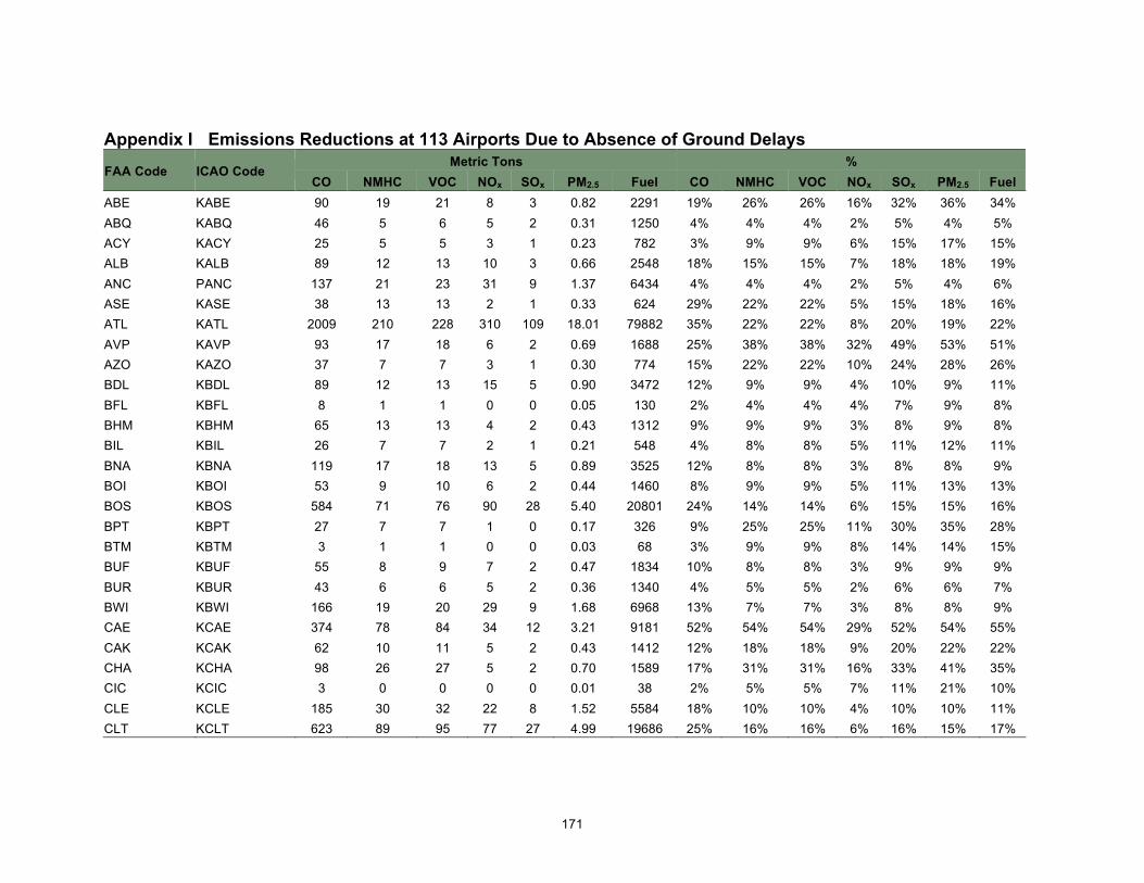
171

Appendix I Emissions Reductions at 113 Airports Due to Absence of Ground Delays Metric Tons %

FAA Code ICAO Code CO NMHC VOC NOx SOx PM2.5 Fuel CO NMHC VOC NOx SOx PM2.5 Fuel

ABE KABE 90 19 21 8 3 0.82 2291 19% 26% 26% 16% 32% 36% 34% ABQ KABQ 46 5 6 5 2 0.31 1250 4% 4% 4% 2% 5% 4% 5% ACY KACY 25 5 5 3 1 0.23 782 3% 9% 9% 6% 15% 17% 15% ALB KALB 89 12 13 10 3 0.66 2548 18% 15% 15% 7% 18% 18% 19% ANC PANC 137 21 23 31 9 1.37 6434 4% 4% 4% 2% 5% 4% 6% ASE KASE 38 13 13 2 1 0.33 624 29% 22% 22% 5% 15% 18% 16% ATL KATL 2009 210 228 310 109 18.01 79882 35% 22% 22% 8% 20% 19% 22% AVP KAVP 93 17 18 6 2 0.69 1688 25% 38% 38% 32% 49% 53% 51% AZO KAZO 37 7 7 3 1 0.30 774 15% 22% 22% 10% 24% 28% 26% BDL KBDL 89 12 13 15 5 0.90 3472 12% 9% 9% 4% 10% 9% 11% BFL KBFL 8 1 1 0 0 0.05 130 2% 4% 4% 4% 7% 9% 8% BHM KBHM 65 13 13 4 2 0.43 1312 9% 9% 9% 3% 8% 9% 8% BIL KBIL 26 7 7 2 1 0.21 548 4% 8% 8% 5% 11% 12% 11% BNA KBNA 119 17 18 13 5 0.89 3525 12% 8% 8% 3% 8% 8% 9% BOI KBOI 53 9 10 6 2 0.44 1460 8% 9% 9% 5% 11% 13% 13% BOS KBOS 584 71 76 90 28 5.40 20801 24% 14% 14% 6% 15% 15% 16% BPT KBPT 27 7 7 1 0 0.17 326 9% 25% 25% 11% 30% 35% 28% BTM KBTM 3 1 1 0 0 0.03 68 3% 9% 9% 8% 14% 14% 15% BUF KBUF 55 8 9 7 2 0.47 1834 10% 8% 8% 3% 9% 9% 9% BUR KBUR 43 6 6 5 2 0.36 1340 4% 5% 5% 2% 6% 6% 7% BWI KBWI 166 19 20 29 9 1.68 6968 13% 7% 7% 3% 8% 8% 9% CAE KCAE 374 78 84 34 12 3.21 9181 52% 54% 54% 29% 52% 54% 55% CAK KCAK 62 10 11 5 2 0.43 1412 12% 18% 18% 9% 20% 22% 22% CHA KCHA 98 26 27 5 2 0.70 1589 17% 31% 31% 16% 33% 41% 35% CIC KCIC 3 0 0 0 0 0.01 38 2% 5% 5% 7% 11% 21% 10% CLE KCLE 185 30 32 22 8 1.52 5584 18% 10% 10% 4% 10% 10% 11% CLT KCLT 623 89 95 77 27 4.99 19686 25% 16% 16% 6% 16% 15% 17%

172

Metric Tons % FAA Code ICAO Code

CO NMHC VOC NOx SOx PM2.5 Fuel CO NMHC VOC NOx SOx PM2.5 Fuel CMH KCMH 173 33 34 20 7 1.47 5051 19% 18% 18% 6% 16% 18% 17% COS KCOS 75 13 14 7 2 0.51 1787 9% 14% 14% 7% 16% 17% 17% CRW KCRW 126 22 23 6 2 0.69 1741 26% 33% 33% 20% 39% 43% 42% CVG KCVG 451 142 154 52 19 5.59 14088 25% 29% 29% 6% 15% 17% 17% DAL KDAL 73 15 15 6 2 0.56 1657 5% 6% 6% 2% 6% 8% 7% DAY KDAY 62 10 11 8 3 0.58 2266 9% 9% 9% 4% 11% 11% 12% DCA KDCA 302 28 30 49 16 2.81 11935 28% 13% 13% 6% 14% 14% 16% DEN KDEN 532 71 78 70 24 4.73 17453 18% 10% 10% 4% 10% 10% 12% DFW KDFW 1201 80 87 209 74 10.26 54390 31% 15% 15% 7% 18% 17% 19% DLH KDLH 10 2 2 1 0 0.09 234 4% 8% 8% 4% 10% 9% 11% DTW KDTW 562 91 99 98 34 7.56 25282 22% 13% 13% 5% 14% 12% 15% ELP KELP 39 6 6 3 1 0.23 823 8% 6% 6% 2% 5% 6% 5% ERI KERI 25 6 6 1 1 0.19 391 14% 19% 19% 12% 23% 27% 25% EVV KEVV 31 6 6 2 1 0.21 478 10% 16% 16% 8% 17% 22% 19% EWR KEWR 1360 171 186 247 77 14.27 56382 40% 24% 24% 10% 25% 25% 27% FAI PAFA 13 2 2 1 0 0.09 273 3% 3% 3% 2% 4% 5% 4% FAT KFAT 28 4 4 2 1 0.17 677 4% 8% 8% 6% 13% 13% 14% FAY KFAY 73 10 11 4 2 0.43 1238 30% 43% 43% 36% 53% 57% 56% FNT KFNT 83 15 16 8 3 0.76 2239 22% 28% 28% 13% 31% 34% 33% GEG KGEG 39 5 6 6 2 0.35 1327 9% 8% 8% 5% 11% 12% 13% GRR KGRR 107 19 20 9 3 0.81 2422 17% 19% 19% 7% 18% 21% 20% GSO KGSO 143 27 28 12 5 1.09 3347 23% 22% 22% 8% 20% 24% 23% GSP KGSP 165 24 26 14 5 1.21 4012 50% 35% 36% 17% 34% 37% 37% HLN KHLN 7 1 1 0 0 0.04 85 3% 5% 5% 5% 8% 9% 9% HOU KHOU 80 14 14 7 3 0.59 1974 6% 7% 6% 2% 6% 6% 6% HPN KHPN 155 49 50 10 4 1.56 3023 19% 19% 19% 8% 18% 22% 19% HTS KHTS 43 9 9 3 1 0.29 799 19% 40% 39% 34% 51% 56% 52% HVN KHVN 9 2 2 1 0 0.08 186 4% 15% 15% 12% 22% 28% 22%

173


CO NMHC VOC NOx SOx PM2.5 Fuel CO NMHC VOC NOx SOx PM2.5 Fuel IAD KIAD 540 91 95 77 25 5.33 18365 22% 15% 15% 5% 13% 13% 15% IAH KIAH 884 101 109 116 42 7.98 31211 30% 17% 17% 6% 16% 16% 18% IND KIND 234 51 55 30 10 2.45 7539 17% 11% 11% 3% 10% 12% 11% IPL KIPL 5 1 1 0 0 0.02 56 2% 8% 8% 9% 14% 26% 12% ISP KISP 34 6 6 3 1 0.33 859 5% 9% 9% 3% 9% 10% 10% IYK KIYK 2 0 0 0 0 0.01 49 2% 2% 2% 13% 19% 29% 20% JFK KJFK 1356 149 162 309 91 14.94 67039 37% 23% 23% 9% 23% 21% 25% LAN KLAN 42 10 11 5 1 0.40 1014 9% 16% 16% 14% 26% 21% 24% LAS KLAS 652 72 75 145 25 5.76 22492 18% 13% 13% 7% 17% 12% 14% LAX KLAX 840 88 95 221 39 7.21 31552 24% 12% 12% 6% 15% 10% 12% LGA KLGA 857 91 98 168 31 7.93 32713 40% 24% 24% 12% 26% 23% 25% LGB KLGB 25 3 3 7 1 0.20 753 2% 4% 4% 5% 10% 6% 6% MCN KMCN 54 9 10 2 0 0.22 452 28% 43% 42% 31% 45% 51% 46% MDT KMDT 215 59 64 21 5 2.20 5290 44% 44% 44% 25% 45% 46% 46% MDW KMDW 226 32 34 50 9 2.21 7039 18% 10% 10% 6% 14% 9% 10% MEM KMEM 557 142 154 112 19 5.94 15298 21% 11% 11% 6% 14% 11% 11% MFR KMFR 9 1 1 1 0 0.05 173 5% 6% 6% 10% 16% 10% 10% MHT KMHT 72 10 11 15 3 0.60 2142 19% 10% 10% 7% 15% 11% 12% MKE KMKE 158 30 32 26 5 1.23 4067 17% 10% 10% 6% 14% 9% 10% MOD KMOD 5 1 1 0 0 0.02 69 2% 8% 8% 12% 17% 26% 13% MSN KMSN 65 13 13 8 2 0.55 1626 12% 17% 17% 10% 22% 20% 20% MSP KMSP 744 114 123 170 31 9.37 30695 31% 17% 16% 9% 20% 15% 18% OAK KOAK 151 22 24 41 7 1.36 4417 9% 6% 6% 5% 11% 7% 7% ONT KONT 73 12 13 20 3 0.60 1994 11% 6% 6% 5% 11% 5% 6% ORD KORD 2114 183 198 489 86 18.63 86439 36% 20% 20% 11% 24% 19% 22% ORF KORF 132 20 21 17 4 0.98 3537 25% 21% 21% 11% 24% 22% 22% OXR KOXR 4 1 1 0 0 0.01 35 1% 4% 4% 9% 11% 13% 6% PDX KPDX 122 14 15 32 5 0.98 3653 12% 7% 7% 5% 11% 7% 7%

174


CO NMHC VOC NOx SOx PM2.5 Fuel CO NMHC VOC NOx SOx PM2.5 Fuel PHF KPHF 134 20 21 12 3 0.92 2977 17% 32% 32% 24% 42% 50% 43% PHL KPHL 1251 180 194 230 41 12.11 43716 40% 24% 23% 14% 28% 22% 27% PHX KPHX 698 70 75 157 27 5.98 24317 26% 13% 13% 8% 18% 12% 15% PIH KPIH 5 1 1 0 0 0.02 51 2% 6% 6% 12% 15% 17% 10% PIT KPIT 208 34 36 36 7 1.63 5786 19% 12% 12% 7% 15% 11% 12% PSP KPSP 24 5 5 4 1 0.17 515 7% 9% 9% 6% 14% 9% 9% PVD KPVD 55 6 7 13 2 0.40 1573 13% 8% 8% 5% 12% 7% 8% PWM KPWM 122 17 18 17 3 0.92 3587 33% 32% 32% 24% 41% 38% 42% RDU KRDU 165 27 28 27 5 1.16 4041 16% 12% 12% 6% 14% 10% 10% RIC KRIC 162 33 35 20 4 1.24 4015 28% 22% 22% 11% 25% 20% 23% RNO KRNO 76 10 10 15 3 0.57 2083 11% 10% 10% 7% 15% 11% 12% ROA KROA 315 56 59 25 6 2.25 6614 47% 57% 57% 46% 64% 66% 67% ROC KROC 282 46 48 40 8 2.58 9138 40% 38% 38% 22% 41% 43% 42% SAN KSAN 155 16 17 42 7 1.42 5546 16% 9% 9% 6% 13% 8% 9% SAT KSAT 100 18 18 18 4 0.74 2358 11% 8% 8% 6% 12% 7% 8% SDF KSDF 417 182 198 65 12 5.67 11065 29% 21% 21% 9% 20% 14% 18% SEA KSEA 294 23 25 82 14 2.73 11475 21% 10% 10% 6% 14% 9% 11% SFO KSFO 436 45 48 126 21 4.14 16969 21% 11% 11% 7% 15% 10% 12% SJC KSJC 101 13 13 26 5 0.82 3010 13% 7% 7% 5% 11% 7% 7% SLC KSLC 427 48 51 78 15 3.45 12015 21% 13% 13% 9% 18% 12% 14% SMF KSMF 123 12 13 28 5 1.09 3992 19% 11% 11% 7% 16% 12% 13% SNA KSNA 146 22 22 30 5 1.44 4620 11% 11% 11% 7% 15% 11% 12% STL KSTL 185 23 25 36 7 1.19 5245 17% 9% 9% 6% 13% 8% 9% SWF KSWF 21 5 5 3 1 0.19 531 5% 8% 8% 5% 13% 12% 10% SYR KSYR 221 31 33 29 6 1.80 6516 36% 36% 36% 22% 40% 43% 41% TOL KTOL 376 60 64 61 14 3.98 17311 52% 47% 47% 49% 70% 66% 72% TRI KTRI 124 31 31 8 2 0.93 2179 24% 43% 42% 28% 47% 52% 48% TUS KTUS 39 5 5 8 2 0.19 821 4% 5% 5% 5% 11% 5% 6%

175


CO NMHC VOC NOx SOx PM2.5 Fuel CO NMHC VOC NOx SOx PM2.5 Fuel TYS KTYS 123 27 28 10 2 0.86 2190 16% 19% 19% 13% 24% 18% 22% VIS KVIS 3 1 1 0 0 0.01 20 2% 6% 6% 6% 9% 17% 8%

176

Appendix J Comparison of EDMS Aircraft Emissions with Other Sectors in the 2002 NEI -- for NAAs

It is interesting to consider the aircraft LTO emissions during the period June 2005 through May 2006 in the context of other mobile source emission categories in NAAs. Table J.1 through Table J.5 present NOx, PM2.5, VOC, CO, and SO2 emissions for 2002 in the 118 NAAs for mobile source categories, including aircraft at the 148 commercial service airports (2002 is the base year for non-aircraft emissions and 2005 is the base year for aircraft emissions).

Table J.1: Nonattainment area annual NOx emission levels for mobile source categories for 2002 a,b,c,d. Units are metric tons.

Source NOx Aircraft 73,152 Recreational Marine Diesel

13,520


398,338


755,208


105,414

Small Nonroad SI 83,735 Recreational Marine SI 27,661 SI Recreational Vehicles

2,411


168,424

Locomotive 330,894 Total Off-Highway 1,958,755 Highway non-diesel 2,229,330 Highway Diesel 1,683,882 Total Highway 3,913,213 Total Mobile Sources 5,871,967


177

Table J.2: Nonattainment area annual PM2.5 emission levels for mobile source categories for 2002. Units are metric tons.

Source PM2.5 Aircraft 1,948 Recreational Marine Diesel

368


14,342


65,572


5,475


6,488


2,668


833

Locomotive 8,301 Total Off-Highway 120,299 Highway non-diesel 28,504 Highway Diesel 42,729 Total Highway 71,233 Total Mobile Sources

191,532

Table J.3: Nonattainment area annual VOC emission levels for mobile source categories for 2002. Units are metric tons.

Source VOC Aircraft 33,681 Recreational Marine Diesel

725


10,408


87,844


3,356


318,161


103,561

178

Source VOC Large Nonroad SI (>25hp)

42,398

Locomotive 15,380 Total Off-Highway 1,246,791 Highway non-diesel

2,282,459

Highway Diesel 90,383 Total Highway 2,372,841 Total Mobile Sources

3,619,633

Table J.4: Nonattainment area annual CO emission levels for mobile source categories for 2002. Units are metric tons.

Source CO Aircraft 162,469 Recreational Marine Diesel

2,496


72,673


387,593


13,404

Small Nonroad SI 8,469,535 Recreational Marine SI

1,000,876


283,280


764,390

Locomotive 41,848 Total Off-Highway 11,198,562 Highway non-diesel 28,119,702 Highway Diesel 445,335 Total Highway 28,565,037 Total Mobile Sources

39,763,600

Table J.5: Nonattainment area annual SO2 emission levels for mobile source categories for 2002. Units are metric tons.

Source SO2 Aircraft 7,743

Recreational Marine 1,643

179

Source SO2 Diesel


51,177


67,566


68,042


670


169


286

Locomotive 20,970 Total Off-Highway 220,525 Highway non-diesel 70,025 Highway Diesel 30,979 Total Highway 101,004 Total Mobile Sources 321,529

aircraft impacts on local and regional air quality in the

Documents