airborne laser scanning for riverbank erosion assessment

www.elsevier.com/locate/rse

Remote Sensing of Environm

Airborne laser scanning for riverbank erosion assessment

David P. Thomaa,T, Satish C. Guptab, Marvin E. Bauerc, C.E. Kirchoff d

aUSDA-ARS Southwest Watershed Research Center, 2000 E. Allen Road, Tucson, AZ 85719, United StatesbDepartment of Soil, Water, and Climate, 1991 Upper Buford Circle, St. Paul, MN 55108, United States

cDepartment of Forest Resources, 1530 Cleveland Ave. N., St. Paul, MN 55108, United StatesdUniversity of Minnesota Supercomputing Center, 117 Pleasant St. SE, Minneapolis, MN 55455, United States

Received 7 September 2004; received in revised form 10 January 2005; accepted 12 January 2005

Abstract

Worldwide, rivers and streams are negatively impacted by sedimentation. However, there are few broad scale techniques for quantifying

the sources of sediment, i.e. upland vs. river bank erosion. This research was designed to evaluate the use of airborne LIDAR for

characterizing sediment and phosphorus contributions from river bank erosion. The evaluation was done on the main stem of the Blue Earth

River in southern Minnesota. Detailed topographic data were collected on an annual basis in April 2001 and 2002 over a 56 km length of the

river with a helicopter mounted Topeye laser system. The raw database included X, Y, Z coordinates of laser returns sampled from the river

valley with a density of 1–3.3 elevations per m2. Uniform 1 m bare earth digital elevation models were constructed by stripping vegetation

laser returns and interpolation. The two models were differenced to determine volume change over time, which was then converted to mass

wasting by multiplying volume change with bulk density. Mass wasting rates were further converted to sediment load based on percentage of

transportable material in the bank strata. The average difference between LIDAR measured elevations and RTK GPS surveyed elevations on

5 highway bridge surfaces was 2.5 and 8.8 cm for the 2001 and 2002 scans, respectively. The elevation errors were quasi-normally

distributed with standard deviation of 6.7 and 6.1 cm for 2001 and 2002, respectively. No elevation or planimetric corrections were made to

the laser data before calculating mass wasting rates because it was not possible to determine the source of error or if it was uniform within and

between scans. The mass wasting estimate from the LIDAR surveys varied from 23% to 56% of the sediment mass transported past the

downstream gauging station depending on the range of textural material that was entrained once in the river. These estimates are in the range

of values reported in the literature. Total P contribution due to bank erosion from the river reach was estimated to be 201 t/yr.

D 2005 Elsevier Inc. All rights reserved.

Keywords: Sediment pollution; Laser altimetry; LIDAR; Bank erosion

1. Introduction

Bank erosion contribution to suspended sediment load

varies widely from 17% to 93% for rivers studied in

England, Europe and North America (Sekely, Mulla, &

Bauer, 2002). Such a wide range in values is due to many

factors including differences in climate, topography, geol-

ogy, soils, and land management. The National Water

Quality Inventory report (USEPA, 2000) indicates 12% of

assessed rivers and streams in the U.S. are impacted

0034-4257/$ - see front matter D 2005 Elsevier Inc. All rights reserved.

doi:10.1016/j.rse.2005.01.012

T Corresponding author. Tel.: +1 520 670 6381x111; fax: +1 520 670 550.

E-mail address: [email protected] (D.P. Thoma).

negatively by sedimentation. Negative impacts of siltation

include suffocation of fish eggs, decreased light penetration

for photosynthesis, decreased aesthetic value for recrea-

tional uses, and added cost of water treatment.

Agriculture is implicated as the major source for

sediment pollution in many rivers. Phosphorus adsorbed to

soil particles is often delivered with sediment further

contributing to water quality degradation through eutrophi-

cation (Sharpley et al., 2003). However, because of their

diffuse nature, reductions in sediment and phosphorus are

difficult to achieve, but are typically attempted through

implementation of conservation practices. Conservation

tillage and grassed waterways as well as buffer strips at

field edges can reduce sediment and phosphorus transport to

ent 95 (2005) 493–501

D.P. Thoma et al. / Remote Sensing of Environment 95 (2005) 493–501494

surface waters (Gupta & Singh, 1996; Randall et al., 1996).

However, sediment and phosphorus sources in agricultural

landscapes include both bare fields as well as riverbanks in

dynamic fluvial systems. Therefore, determining the pro-

portion of sediment and phosphorus delivered from either of

these sources is a difficult, yet important task for cost

effective implementation of conservation measures, or

engineering solutions for bank erosion.

Airborne laser altimetry has been used in numerous

topographic and land use change detection studies (Huising

& Gomes Pereira, 1998; Irish & Lillycrop, 1999; Krabill et

al., 1999; Murakami et al., 1999; Sallenger et al., 1999).

Laser altimetry has also been used for gully erosion

estimates (Jackson et al., 1988; Ritchie et al., 1994),

earthquake fault mapping (Harding & Berghoff, 2000;

Hudnut et al., 2002), and to map riverbank elevations for

flood management (Pereira & Wicherson, 1999).

As the aircraft moves along a predetermined flight line

the LIDAR system sends many thousands of laser pulses to

the ground each second in a scanning pattern centered on

the flight line. Up to five echoes from each laser pulse are

received by the sensor to compute elevations based on laser

travel times. Typically, the first returned pulse is from the

top of the vegetation canopy while the last is usually the

ground. In situations where the last echo return is not the

ground, filtering must be employed to remove vegetation

elevation data if interest is purely in the bare earth elevation

(Ritchie et al., 1994). Typically, the high density of data

from combinations of multiple passes allows spatial

averaging of elevations without loss of systematic variation

in the landscape surface elevation (Ritchie et al., 1994). An

Inertial Measurement System (IMU) is used to measure

aircraft attitude during the flight which is used to correct for

errors due to roll, pitch and yaw. Most IMU’s have angular

resolutions of approximately 0.01 degree (Fowler, 2000)

which can induce error up to 2.5 cm vertical and 7.4 cm

horizontal at 20 degree scan angle and 375 m flight altitude.

This error represents a large fraction of the LIDAR errors

and cannot be easily removed. Resulting data resolution

depends on aircraft elevation and speed as well as laser

pulse rate, scan width, scan rate, and vegetation cover. Data

collection in the fall or winter during leaf-off conditions

optimizes sampling density and accuracy of bare earth

measurements.

The 6294 km2 Blue Earth River watershed in south

central Minnesota is a good example of a landscape where

non-point source sediment and phosphorus pollution are

prevalent, but difficult to apportion between upland and

stream bank erosion. The 160 km long Blue Earth River has

a mean discharge of 37 m3/s with maximum flood flow of

1699 m3/s and average gradient less than 0.6 m/km. The

Blue Earth River is a major tributary of the Minnesota River

and contributes about 55% of the sediment load carried by

the Minnesota River at Mankato, MN (Payne, 1994; WRC,

2004). The Minnesota Pollution Control Agency (MPCA,

1985) stated that a 40% reduction in sediment load carried

by the Minnesota River would be required to meet federal

water quality standards and beneficial use criteria. Thus far,

the cause of this pollution has been blamed on agricultural

practices in relatively flat upland areas of the watershed.

Therefore, the strategy for controlling these pollutants has

also focused on implementing agricultural practices that

limit delivery of sediments and nutrients to the river

(Randall et al., 1996). However, this strategy may be

ineffective since it is not clear what proportion of the

sediment and nutrient pollution in the Minnesota River is

from upland erosion or stream bank erosion.

Objectives of the study were to 1) evaluate the

capabilities and limitations of LIDAR remote sensing for

river bank erosion, 2) quantify mass wasting and phospho-

rus inputs along a 56 km length of the Blue Earth River,

and 3) estimate the proportion of total annual suspended

sediment and phosphorus loads due to bank erosion.

2. Methods

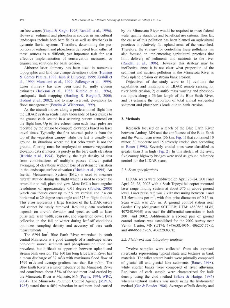
Research focused on a reach of the Blue Earth River

between Amboy, MN and the confluence of the Blue Earth

and the Wantonwan rivers (56 km; Fig. 1) that contained 10

minor, 30 moderate and 15 severely eroded sites according

to Bauer (1998). Severely eroded sites were classified as

greater than 3 m high (Fig. 2). In this stretch of the river,

five county highway bridges were used as ground reference

control for the LIDAR scans.

2.1. Scan specifications

LIDAR scans were conducted on April 23–24, 2001 and

April 26–28, 2002 with a Saab Topeye helicopter mounted

laser range finding system at about 375 m above ground

level. Laser pulse rate was 7 kHz measuring between 1 and

3.3 elevations per m2, with foot print diameters of 0.16 m.

Scan width was 273 m. A ground control station near

Garden City (designated SCHOEB; UTM: 4880562.343N,

407248.996E) was used for differential correction in both

2001 and 2002. Additionally a second pair of ground

control stations was established for the 2002 survey near

Vernon Center, MN (UTM: 4868658.493N, 406207.778E;

and 4868658.526N, 406229.837E).

2.2. Fieldwork and laboratory analysis

Twelve samples were collected from six exposed

riverbanks representing typical strata and textures in bank

materials. The taller stream banks were primarily composed

of glacial till and glacial lake sediments (Bauer, 1998),

while shorter banks were composed of river alluvium.

Replicates of each sample were characterized for bulk

density using the clod method (Blake & Hartge, 1986)

whereas textural analysis was made using the hydrometer

method (Gee & Bauder 1986). Averages of bulk density and

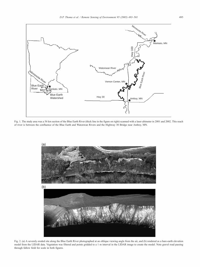
Fig. 2. (a) A severely eroded site along the Blue Earth River photographed at an oblique viewing angle from the air, and (b) rendered as a bare-earth elevation

model from the LIDAR data. Vegetation was filtered and points gridded to a 1 m interval in the LIDAR image to create the model. Note gravel road passing

through fallow field for scale in both figures.

Minnesota RiverBlue Earth

Blue EarthWatershed Hwy 30

Amboy, MN

Vemon Center, MN

Blu

e E

arth

Riv

er

Watonwan River

Hw

y 16

9

Mankato, MN

Minnesota River

River Mankato. MN

Fig. 1. The study area was a 56 km section of the Blue Earth River (thick line in the figure on right) scanned with a laser altimeter in 2001 and 2002. This reach

of river is between the confluence of the Blue Earth and Watonwan Rivers and the Highway 30 Bridge near Amboy, MN.

D.P. Thoma et al. / Remote Sensing of Environment 95 (2005) 493–501 495


textural analysis were used in conjunction with LIDAR

determined volume change to derive mass wasting rates. All

samples were analyzed for extractable phosphorus (Kuo,

1986) using 0.01 M CaCl2, and total P via perchloric acid

digestion (USEPA, 1981).

Elevation accuracy of both annual scans was determined

by comparing the LIDAR scan elevations of bridges

crossing the river to bridge elevations determined by real

time kinematic (RTK) GPS survey in 2002. A total of 137

bridge reference points were collected on 5 highway bridges

that crossed the scanned portion of the Blue Earth River.

Accuracies of LIDAR scan elevations on the bridge surfaces

were determined as the relative difference between a bridge

reference point elevation and the nearest scan point

elevation that fell on the surface.

The planimetric accuracy was determined by matching

bridge edges in the 2001 scan to edges in the 2002 scan.

Edges were determined by linear regression of scan line

points (laser returns) that fell closest to, but still on, the

bridge surface. The average distance between points on the

best fit lines describing the bridge edges in 2001 and 2002

served as an estimate of planimetric shift. The maximum

distances between control stations and bridges used as

reference surfaces were 20.0 and 12.7 km in 2001 and 2002,

respectively, less than the distance that would require

ionospheric corrections (Shrestha et al., 1999).

2.3. Volume and mass change

Raw scanning laser data were differentially corrected and

stripped of vegetation returns using a proprietary smoothing

filter developed by the data provider, Aerotec LLC. Any

last-return point greater than 1.5 m above ambient ground

surface was considered a return from vegetation and was

removed by the algorithm. Because data points were not

uniformly distributed along the flight path due to mirror

rotation and aircraft trajectory, they were gridded to uniform

1 m spacing in both X-and Y-directions before calculating

the volume change. The resulting data product was an

ordered set of 24 million and 30 million X, Y, Z coordinates

for the 2001 and 2002 scans, respectively.

All data points below the 2001 high water mark (stream

stage was higher in 2001 than in 2002 at time of scans) were

eliminated from both data sets manually by digitizing and

clipping to avoid confusing the difference in stream stage

with changes in elevations due to erosion. Elimination of

Table 1

Properties of upland surface soils and river bank materials collected from 12 sam

Bulk density Sand

(Mg/m3) (%)

Bank materials Min 1.46 32.8

Mean 1.83 55.7

Max 2.13 92.4

Surface soil 1.25–1.45a ~10a

a Average physical properties from two common surface soils in the Blue Earth

X,Y data points that were unique to one or the other

uniformly gridded 1 m data sets produced two surface files

(2001 data and 2002 data) with an identical number of X,Y

coordinates over an identical geographic extent that differed

only in the Z (elevation) dimension. The differences in Z

values were determined for every vertex and summed. The

sum was then multiplied by the spatial extent of the scans to

arrive at an estimate of net volume change that occurred due

to erosion or deposition between the two scans.

Mass wasting estimates were made by multipling average

bulk density by the volume change determined from the

LIDAR scans. Similarly, phosphorus load was derived by

multiplying the concentration of extractable and total

phosphorus in sediment samples by the mass of sediment

that eroded into the river.

Sediment and P loads carried by the river were obtained

from the Metropolitan Environmental Services (Heather

Offerman, personal communication). These loads were

measured using equal flow increment auto-sampling at a

gauging station downstream from the scanned river reach.

3. Results

3.1. Properties of bank materials

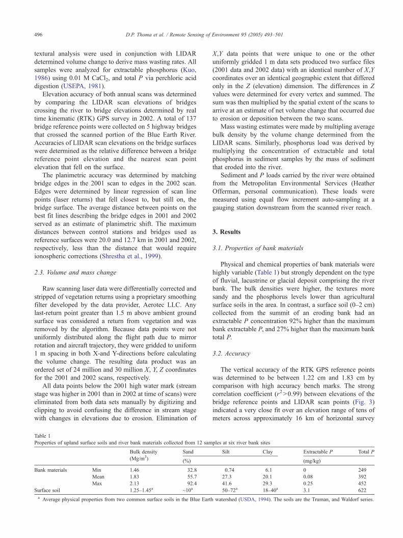
Physical and chemical properties of bank materials were

highly variable (Table 1) but strongly dependent on the type

of fluvial, lacustrine or glacial deposit comprising the river

bank. The bulk densities were higher, the textures more

sandy and the phosphorus levels lower than agricultural

surface soils in the area. In contrast, a surface soil (0–2 cm)

collected from the summit of an eroding bank had an

extractable P concentration 92% higher than the maximum

bank extractable P, and 27% higher than the maximum bank

total P.

3.2. Accuracy

The vertical accuracy of the RTK GPS reference points

was determined to be between 1.22 cm and 1.83 cm by

comparison with high accuracy bench marks. The strong

correlation coefficient (r2N0.99) between elevations of the

bridge reference points and LIDAR scan points (Fig. 3)

indicated a very close fit over an elevation range of tens of

meters across approximately 16 km of horizontal survey

ples at six river bank sites

Silt Clay Extractable P Total P

(mg/kg)

0.74 6.1 0 249

27.3 20.1 0.08 392

41.6 29.3 0.25 452

50–72a 18–40a 3.1 622

watershed (USDA, 1994). The soils are the Truman, and Waldorf series.

100-10-20-30

30

20

10

0

2001 elevation error (cm)

Fre

quen

cy

50403020100-10

60

50

40

30

20

10

0

2002 elevation error (cm)F

requ

ency

(b)

(a)

Fig. 4. Normal curves superimposed on distributions of elevation errors for

LIDAR scans relative to 137 RTK GPS survey reference points collected on

5 bridges spanning the Blue Earth River. (a) 2001 with mean error 2.5 cm

and 99% confidence interval (CI) {1.043, 4.027}, (b) 2002 with mean 8.8

cm and 99% CI {7.715, 9.793}. Lack of CI overlap indicates the error

means are statistically different.

Table 2

Descriptive statistics for elevation error in the 2001 and 2002 LIDAR scans

2001 2002

Mean (cm) 2.5 8.8

Median (cm) 4.2 8.9

Mode (cm) 4.2 10.7

Stdev (cm) 6.7 6.1

Variance(cm2) 44.4 37.6

RMSE 6.7 6.1

99% Confidence interval for mean (cm) {1.04–4.03} {7.72–9.79}

Errors were computed as RTK GPS survey elevations minus elevations of

the nearest LIDAR point on five highway bridges crossing the Blue Earth

River. The total number of observations considered in this analysis was

137.

2001y = 0.9953x + 1.3838

R2 = 0.9952

2002y = 0.998x + 0.5051

R2 = 0.9980

270

275

280

285

290

295

300

305

310

270 275 280 285 290 295 300 305 310

RTK GPS elevation (m)

LID

AR

ele

vati

on

(m

)

2001 2002 1 to1linear fit 2001 linear fit 2002

Hwy 13

Hwy 10

Hwy 169

Hwy 30

Hwy 34

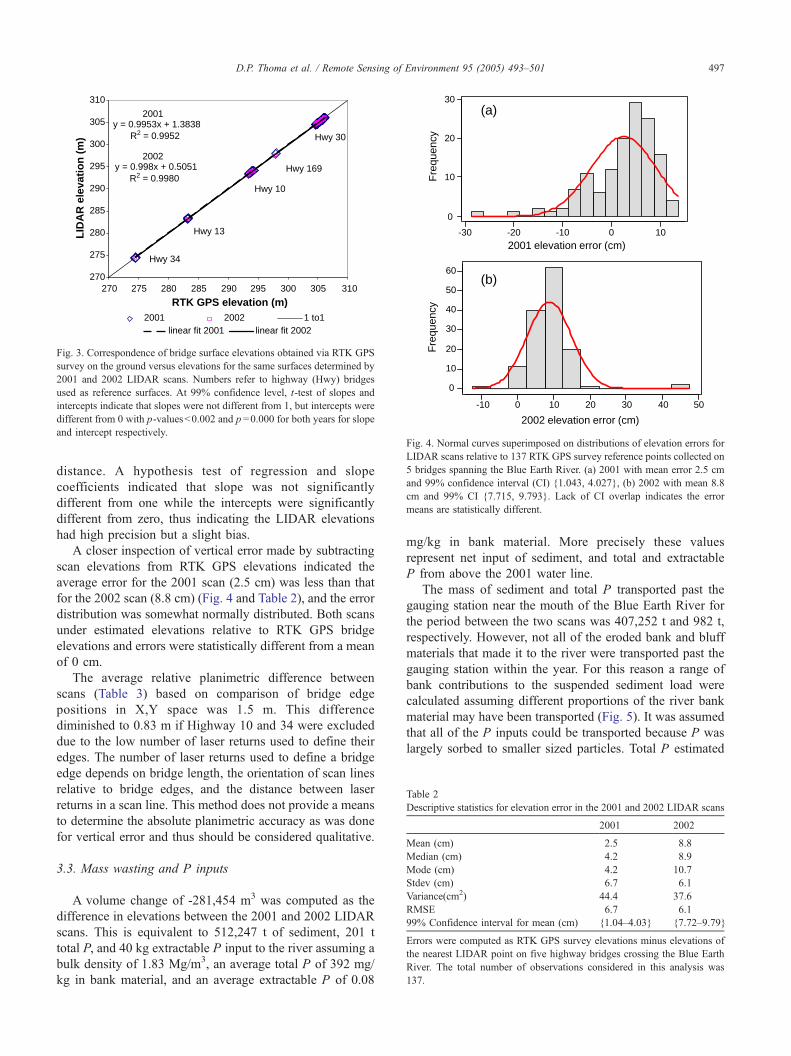
Fig. 3. Correspondence of bridge surface elevations obtained via RTK GPS

survey on the ground versus elevations for the same surfaces determined by

2001 and 2002 LIDAR scans. Numbers refer to highway (Hwy) bridges

used as reference surfaces. At 99% confidence level, t-test of slopes and

intercepts indicate that slopes were not different from 1, but intercepts were

different from 0 with p-valuesb0.002 and p =0.000 for both years for slope

and intercept respectively.


distance. A hypothesis test of regression and slope

coefficients indicated that slope was not significantly

different from one while the intercepts were significantly

different from zero, thus indicating the LIDAR elevations

had high precision but a slight bias.

A closer inspection of vertical error made by subtracting

scan elevations from RTK GPS elevations indicated the

average error for the 2001 scan (2.5 cm) was less than that

for the 2002 scan (8.8 cm) (Fig. 4 and Table 2), and the error

distribution was somewhat normally distributed. Both scans

under estimated elevations relative to RTK GPS bridge

elevations and errors were statistically different from a mean

of 0 cm.

The average relative planimetric difference between

scans (Table 3) based on comparison of bridge edge

positions in X,Y space was 1.5 m. This difference

diminished to 0.83 m if Highway 10 and 34 were excluded

due to the low number of laser returns used to define their

edges. The number of laser returns used to define a bridge

edge depends on bridge length, the orientation of scan lines

relative to bridge edges, and the distance between laser

returns in a scan line. This method does not provide a means

to determine the absolute planimetric accuracy as was done

for vertical error and thus should be considered qualitative.

3.3. Mass wasting and P inputs

A volume change of -281,454 m3 was computed as the

difference in elevations between the 2001 and 2002 LIDAR

scans. This is equivalent to 512,247 t of sediment, 201 t

total P, and 40 kg extractable P input to the river assuming a

bulk density of 1.83 Mg/m3, an average total P of 392 mg/

kg in bank material, and an average extractable P of 0.08

mg/kg in bank material. More precisely these values

represent net input of sediment, and total and extractable

P from above the 2001 water line.

The mass of sediment and total P transported past the

gauging station near the mouth of the Blue Earth River for

the period between the two scans was 407,252 t and 982 t,

respectively. However, not all of the eroded bank and bluff

materials that made it to the river were transported past the

gauging station within the year. For this reason a range of

bank contributions to the suspended sediment load were

calculated assuming different proportions of the river bank

material may have been transported (Fig. 5). It was assumed

that all of the P inputs could be transported because P was

largely sorbed to smaller sized particles. Total P estimated

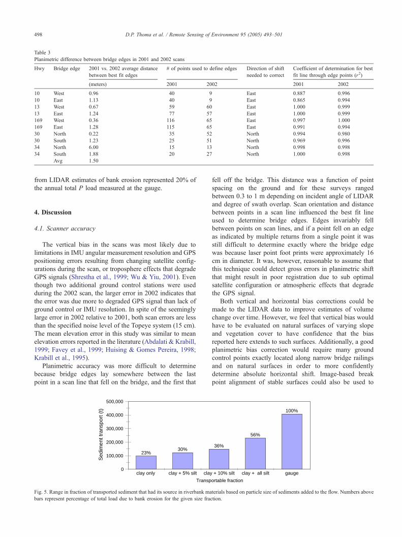
Table 3

Planimetric difference between bridge edges in 2001 and 2002 scans

Hwy Bridge edge 2001 vs. 2002 average distance

between best fit edges

# of points used to define edges Direction of shift

needed to correct

Coefficient of determination for best

fit line through edge points (r2)

(meters) 2001 2002 2001 2002

10 West 0.96 40 9 East 0.887 0.996

10 East 1.13 40 9 East 0.865 0.994

13 West 0.67 59 60 East 1.000 0.999

13 East 1.24 77 57 East 1.000 0.999

169 West 0.36 116 65 East 0.997 1.000

169 East 1.28 115 65 East 0.991 0.994

30 North 0.22 35 52 North 0.994 0.980

30 South 1.23 25 51 North 0.969 0.996

34 North 6.00 15 13 North 0.998 0.998

34 South 1.88 20 27 North 1.000 0.998

Avg 1.50


from LIDAR estimates of bank erosion represented 20% of

the annual total P load measured at the gauge.

4. Discussion

4.1. Scanner accuracy

The vertical bias in the scans was most likely due to

limitations in IMU angular measurement resolution and GPS

positioning errors resulting from changing satellite config-

urations during the scan, or troposphere effects that degrade

GPS signals (Shrestha et al., 1999; Wu & Yiu, 2001). Even

though two additional ground control stations were used

during the 2002 scan, the larger error in 2002 indicates that

the error was due more to degraded GPS signal than lack of

ground control or IMU resolution. In spite of the seemingly

large error in 2002 relative to 2001, both scan errors are less

than the specified noise level of the Topeye system (15 cm).

The mean elevation error in this study was similar to mean

elevation errors reported in the literature (Abdalati & Krabill,

1999; Favey et al., 1999; Huising & Gomes Pereira, 1998;

Krabill et al., 1995).

Planimetric accuracy was more difficult to determine

because bridge edges lay somewhere between the last

point in a scan line that fell on the bridge, and the first that

0

100,000

200,000

300,000

400,000

500,000

Sed

imen

t tra

nspo

rt (

t)

clay only clay + 5% silt clay

Transp

23%30%

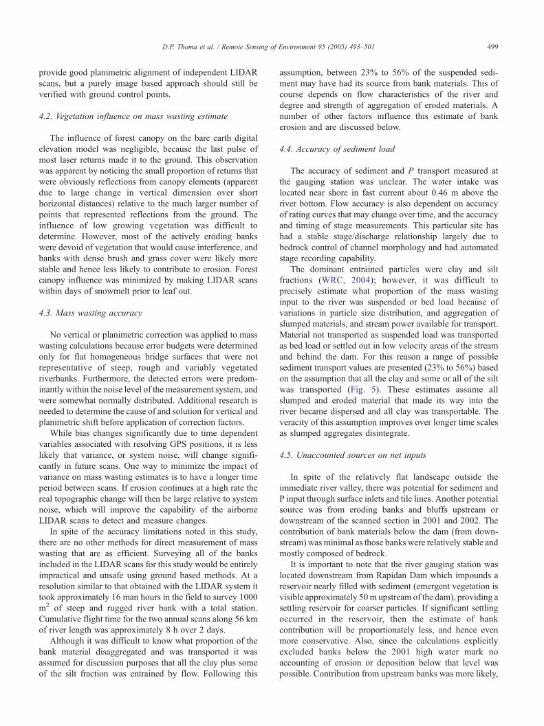
Fig. 5. Range in fraction of transported sediment that had its source in riverbank ma

bars represent percentage of total load due to bank erosion for the given size frac

fell off the bridge. This distance was a function of point

spacing on the ground and for these surveys ranged

between 0.3 to 1 m depending on incident angle of LIDAR

and degree of swath overlap. Scan orientation and distance

between points in a scan line influenced the best fit line

used to determine bridge edges. Edges invariably fell

between points on scan lines, and if a point fell on an edge

as indicated by multiple returns from a single point it was

still difficult to determine exactly where the bridge edge

was because laser point foot prints were approximately 16

cm in diameter. It was, however, reasonable to assume that

this technique could detect gross errors in planimetric shift

that might result in poor registration due to sub optimal

satellite configuration or atmospheric effects that degrade

the GPS signal.

Both vertical and horizontal bias corrections could be

made to the LIDAR data to improve estimates of volume

change over time. However, we feel that vertical bias would

have to be evaluated on natural surfaces of varying slope

and vegetation cover to have confidence that the bias

reported here extends to such surfaces. Additionally, a good

planimetric bias correction would require many ground

control points exactly located along narrow bridge railings

and on natural surfaces in order to more confidently

determine absolute horizontal shift. Image-based break

point alignment of stable surfaces could also be used to

+ 10% silt clay + all silt gauge

ortable fraction

36%

56%

100%

terials based on particle size of sediments added to the flow. Numbers above

tion.


provide good planimetric alignment of independent LIDAR

scans, but a purely image based approach should still be

verified with ground control points.

4.2. Vegetation influence on mass wasting estimate

The influence of forest canopy on the bare earth digital

elevation model was negligible, because the last pulse of

most laser returns made it to the ground. This observation

was apparent by noticing the small proportion of returns that

were obviously reflections from canopy elements (apparent

due to large change in vertical dimension over short

horizontal distances) relative to the much larger number of

points that represented reflections from the ground. The

influence of low growing vegetation was difficult to

determine. However, most of the actively eroding banks

were devoid of vegetation that would cause interference, and

banks with dense brush and grass cover were likely more

stable and hence less likely to contribute to erosion. Forest

canopy influence was minimized by making LIDAR scans

within days of snowmelt prior to leaf out.

4.3. Mass wasting accuracy

No vertical or planimetric correction was applied to mass

wasting calculations because error budgets were determined

only for flat homogeneous bridge surfaces that were not

representative of steep, rough and variably vegetated

riverbanks. Furthermore, the detected errors were predom-

inantly within the noise level of the measurement system, and

were somewhat normally distributed. Additional research is

needed to determine the cause of and solution for vertical and

planimetric shift before application of correction factors.

While bias changes significantly due to time dependent

variables associated with resolving GPS positions, it is less

likely that variance, or system noise, will change signifi-

cantly in future scans. One way to minimize the impact of

variance on mass wasting estimates is to have a longer time

period between scans. If erosion continues at a high rate the

real topographic change will then be large relative to system

noise, which will improve the capability of the airborne

LIDAR scans to detect and measure changes.

In spite of the accuracy limitations noted in this study,

there are no other methods for direct measurement of mass

wasting that are as efficient. Surveying all of the banks

included in the LIDAR scans for this study would be entirely

impractical and unsafe using ground based methods. At a

resolution similar to that obtained with the LIDAR system it

took approximately 16 man hours in the field to survey 1000

m2 of steep and rugged river bank with a total station.

Cumulative flight time for the two annual scans along 56 km

of river length was approximately 8 h over 2 days.

Although it was difficult to know what proportion of the

bank material disaggregated and was transported it was

assumed for discussion purposes that all the clay plus some

of the silt fraction was entrained by flow. Following this

assumption, between 23% to 56% of the suspended sedi-

ment may have had its source from bank materials. This of

course depends on flow characteristics of the river and

degree and strength of aggregation of eroded materials. A

number of other factors influence this estimate of bank

erosion and are discussed below.

4.4. Accuracy of sediment load

The accuracy of sediment and P transport measured at

the gauging station was unclear. The water intake was

located near shore in fast current about 0.46 m above the

river bottom. Flow accuracy is also dependent on accuracy

of rating curves that may change over time, and the accuracy

and timing of stage measurements. This particular site has

had a stable stage/discharge relationship largely due to

bedrock control of channel morphology and had automated

stage recording capability.

The dominant entrained particles were clay and silt

fractions (WRC, 2004); however, it was difficult to

precisely estimate what proportion of the mass wasting

input to the river was suspended or bed load because of

variations in particle size distribution, and aggregation of

slumped materials, and stream power available for transport.

Material not transported as suspended load was transported

as bed load or settled out in low velocity areas of the stream

and behind the dam. For this reason a range of possible

sediment transport values are presented (23% to 56%) based

on the assumption that all the clay and some or all of the silt

was transported (Fig. 5). These estimates assume all

slumped and eroded material that made its way into the

river became dispersed and all clay was transportable. The

veracity of this assumption improves over longer time scales

as slumped aggregates disintegrate.

4.5. Unaccounted sources on net inputs

In spite of the relatively flat landscape outside the

immediate river valley, there was potential for sediment and

P input through surface inlets and tile lines. Another potential

source was from eroding banks and bluffs upstream or

downstream of the scanned section in 2001 and 2002. The

contribution of bank materials below the dam (from down-

stream) wasminimal as those banks were relatively stable and

mostly composed of bedrock.

It is important to note that the river gauging station was

located downstream from Rapidan Dam which impounds a

reservoir nearly filled with sediment (emergent vegetation is

visible approximately 50m upstream of the dam), providing a

settling reservoir for coarser particles. If significant settling

occurred in the reservoir, then the estimate of bank

contribution will be proportionately less, and hence even

more conservative. Also, since the calculations explicitly

excluded banks below the 2001 high water mark no

accounting of erosion or deposition below that level was

possible. Contribution from upstream banks was more likely,


but was assumed to be small as the most actively eroding

banks were contained within the scanned reach. Of 18

severely eroding sites along 157 km of the Blue Earth River,

Bauer (1998) identified only two that were above or below

the scanned section in this study.

4.6. Interpretation of mass wasting and P inputs

In this study, the highest mass wasting estimate ranged

up to 56% of the transported load measured by a

downstream gauging station, while the total P contribution

was estimated at 20% from bank erosion. This does not

imply that these percentages are directly attributable to

bank erosion, which would require a rigorous accounting

of bed and entrained loads bounding the scanned reach.

Rather, these percentages are presented relative to the

gauge load (1) to establish that the estimates using

LIDAR are reasonable and (2) to further the discussion

on how LIDAR could be useful in developing sediment

budgets.

It is instructive to interpret the effect of bank erosion on

sediment yield from the watershed. The annual load divided

by watershed area represents the sediment yield. Based on

the gauge data, the annual sediment and total P yields for

the Blue Earth River watershed in 2001 were 647 kg/ha and

1.6 kg/ha, respectively. By subtracting the contribution of

bank erosion from the total load the misappropriation of

sediment yield to uplands that may have had its source in

banks was determined to be between 149 and 362 kg/ha for

sediment and 0.31 kg/ha for total P. Results such as these

could have important bearing on land management at the

watershed scale.

4.7. Role of LIDAR in soil erosion measurement

Due to weaknesses in current upland soil erosion models

that fail to adequately account for gully erosion, bank

erosion, sediment delivery from field to stream, and in

stream sediment storage, alternative tools are needed for

upland soil erosion measurement and prediction. With

LIDAR technology, it is now possible that significant

improvements could be made for large areas by developing

sediment budgets that determine upland erosion by differ-

ence. This would represent a shift from empirically based

upland erosion modeling to a physically based sediment

budget approach (Trimble & Crosson, 2000). Airborne

LIDAR could provide a unique role in erosion prediction

technology for large areas and long time frames that will

improve geomorphic and watershed scale erosion estimates

that are strongly scale dependent (Osterkamp & Toy, 1997).

5. Conclusions

This study demonstrated the potential of LIDAR to

partition non-point source sediment pollution from bank

erosion. Using two scans made one year apart on the Blue

Earth River in southern Minnesota estimated bank erosion

inputs represented up to 56% and 20% of transported

sediment and total P measured at a river gauging station.

However, this does not mean all sloughed bank material

made it to the gauging station in that year. These estimates

are based on the volume change in river valley walls

between 2001 and 2002 above the high waterline in 2001.

Erosion or deposition below the high waterline could not be

quantified because the laser wavelengths used are strongly

absorbed by water.

Interpretation of mass wasting estimates derived from

scanner data must be made in light of several factors that

affect accuracy. These include the inherent errors in both

laser altimetry measurements (vertical and planimetric

shifts) and river gauging station measurements (accuracy

in rating curve and stage measurements). Bias in scan

elevations and planimetric accuracy may be corrected if

systematic error can be separated from system noise. For

the two annual scans used in this study the vertical error

was within laser manufacturer specifications and no

consistent bias was detected in planimetric shift. While

there were sources of error in partitioning sediment using

this method, it should be recognized that there are no

conventional means of surveying at this level of accuracy

for such extensive areas.

This study illustrated how scanning laser altimetry could

be used in conjunction with river gauging station data to

estimate the contribution of eroding bank materials to total

suspended load. Operationally, resource managers at federal,

state and local levels could use this technology to determine

allocation of resources to projects with the greatest potential

for pollution abatement. In addition, isolating stream bank

inputs and upland contributions by difference with total

sediment load can help determine effectiveness of upland

soil erosion control efforts.

Acknowledgements

This research was partially supported with funds from the

Minnesota Corn and Soybean Research and Promotion

Councils, the University of Minnesota Water Resources

Research Center and the University of Minnesota Graduate

School. The senior author’s salary was partially supported

by the National Needs Fellowship Program of the United

States Department of Agriculture.

References

Abdalati, W., & Krabill, W. B. (1999). Calculation of ice velocities in the

Jakobshavn Isbrae area using airborne laser alitmetry. Remote Sensing

Environment, 67, 194–204.

Bauer, D. W. (1998). Stream bank erosion and slumping along the Blue

Earth River. M.S. thesis. University of Minnesota, St. Paul, MN, 77 pp.


Blake, G. R., & Hartge, K. H. (1986). Bulk density, clod method. In A.

Klute (Ed.), Methods of soil analysis: Part 1. Physical and minera-

logical methods, Second ed. Madison, WI: American Society of

Agronomy, Soil Science Society of America.

Favey, E., Geiger, A., Gudmundsson, G. H., & Wher, A. (1999). Evaluating

the potential of an airborne laser-scanning system for measuring volume

changes of glaciers. Geografiska Annaler, 81 A(4), 555–561.

Fowler, R. A. (2000). LIDAR for flood mapping. Earth Observation

Magazine, 9(7), 23–26.

Gee, G. W., & Bauder, J. W. (1986). Particle size analysis, hydrometer

method. In A. Klute (Ed.), Methods of soil analysis: Part 1. Physical

and mineralogical methods , Second ed. Madison, WI: American

Society of Agronomy, Soil Science Society of America.

Gupta, S. C., & Singh, U. B. (1996). A review of non-point source pollution

models: Implications for the Minnesota River Basin. Department of

Soil, Water, and Climate, College of Agricultural, Food, and Environ-

mental Sciences, University of Minnesota, St. Paul, MN. A report

submitted to the Minnesota Department of Agriculture, p. 77.

Harding, D. J., & Berghoff, G. S. (2000). Fault scarp detection beneath

dense vegetation cover: Airborne LIDAR mapping of the Seattle Fault

Zone, Bainbridge Island, Washington State. Proceedings of the

American Society of Photogrammetry and Remote Sensing Annual

Conference, Washington, D.C., May, 2000.

Hudnut, K. W., Borsa, A., Glennie, C., & Minster, J. B. (2002). High-

resolution topography along surface rupture of the 16 October 1999

Hector Mine, California, Earthquake (Mw 7.1) from airborne laser

swath mapping. Bulletin of the Seismological Society of America, 4(92),

1570–1576.

Huising, E. J., & Gomes Pereira, L. M. (1998). Errors and accuracy of laser

data acquired by various laser scanning systems for topographic

applications. ISPRS Journal of Photogrammetry and Remote Sensing,

53, 245–261.

Irish, J. L., & Lillycrop, W. J. (1999). Scanning laser mapping of the coastal

zone: The SHOALS system. ISPRS Journal of Photogrammetry and

Remote Sensing, 54, 123–129.

Jackson, T. J., Ritchie, J. C., White, J., & LeSchack, L. (1988). Airborne

laser profile data for measuring ephemeral gully erosion. Photo-

grammetric Engineering and Remote Sensing, 54(8), 1181–1185.

Krabill, W., Frederick, E., Manizade, S., Martin, C., Sonntag, J., Swift, R.,

et al. (1999). Rapid thinning of parts of the southern Greenland ice

sheet. Science, 283, 1522–1524.

Krabill, W. B., Thomas, R. H., Martin, C. F., Swift, R. N., & Frederick, E. B.

(1995). Accuracy of airborne laser altimetry over the Greenland ice

sheet. International Journal of Remote Sensing, 16(7), 1211–1222.

Kuo, S. (1986). Phosphorus, extraction with water or dilute salt solution. In

A. Klute (Ed.), Methods of soil analysis: Part 1. Physical and

mineralogical methods, Second ed. Madison, WI: American Society

of Agronomy, Soil Science Society of America.

Minnesota Pollution Control Agency (MPCA). (1985). Lower Minnesota

Waste Load Allocation Study. St. Paul, MN7 Author, 190 p.

Murakami, H., Nakagawa, K., Hasegawa, H., Shibata, T., & Iwanami, E.

(1999). Change detection of buildings using an airborne laser

scanner. ISPRS Journal of Photogrammetry and Remote Sensing,

54, 148–152.

Osterkamp, W. R., & Toy, T. J. (1997). Geomorphic considerations for

erosion prediction. Environmental Geology, 29(3/4), 152–157.

Payne, G. A. (1994). Sources and transport of sediment, nutrients, and

oxygen-demanding substances in the Minnesota River Basin, 1989–

1992. Minnesota River Assessment Project Report. Physical and

Chemical Assessment, vol. II. St. Paul, MN7 Minnesota Pollution

Control Agency.

Pereira, L. M. G., & Wicherson, R. J. (1999). Suitability of laser data for

deriving geographical information: A case study in the context of

management of fluvial zones. ISPRS Journal of Photogrammetry and

Remote Sensing, 54, 105–114.

Randall, G. W., Evans, S. D., Moncrief, J. F., & Lueschen, W. E. (1996).

Tillage best management practices for continuous corn in the Minnesota

River Basin. Minnesota Extension Service publication FO-6672-C.

Ritchie, J. C., Grissinger, E. H., Murphey, J. B., & Garbrecht, J. D. (1994).

Measuring channel and gully cross-sections with an airborne laser

altimeter. Hydrological Processes, 8, 237–243.

Sallenger, A. H., Krabill, W., Brock, J., Swift, R., Jansen, J., Manizade, S.,

et al. (1999). Airborne laser study quantifies El Nino-induced coastal

change. EOS Transactions, vol. 80. 8. (pp. 89–93) American Geo-

physical Union.

Sekely, A. C., Mulla, D. J., & Bauer, D. W. (2002). Streambank slumping

and its contribution to the phosphorus and suspended sediment load of

the Blue Earth River Minnesota. Journal of Soil and Water Con-

servation, 57(5), 243–250.

Sharpley, A. N., Daniel, T., Simms, T., Lemunyon, J., Stevens, R., & Parry,

R. (2003). Agricultural Phosphorus and Eutrophication (2nd ed.). U.S.

Dept. of Agriculture, Agricultural Research Service ARS series 149.

Shrestha, R. L., Carter, W. E., Finer, M. L. P., & Satori, M. (1999). Airborne

laser swath mapping: Accuracy assessment for surveying and mapping

applications. Surveying and Land Information Systems, 59(2), 83–94.

Trimble, S. W., & Crosson, P. (2000). U.S. soil erosion rates—myth and

reality. Science, 189, 248–250.

USDA-Soil Conserv. Serv. (1994). Soil survey of Faribault County,

Minnesota. St. Paul, MN7 USDA-SCS.

United States Environmental Protection Agency (USEPA). (1981). Proce-

dures for handling and chemical analysis of sediment and water

Samples. U.S. environmental laboratory. Vicksburg, MS7 U.S. Army

Engineer Water Ways Experiment Station.

United States Environmental Protection Agency (USEPA). (2000). The

Quality of our Nation’s Waters: Water Quality Report. http://www.

epa.gov/305b/2000report/

Water Resources Center (WRC). (2004). State of Minnesota River:

Summary of Surface Water Quality Monitoring 2002–2004. Mankato,

MN7 Water Resources Center, Minnesota State University.

Wu, J., & Yiu, F. (2001). Local height determination using GPS-

monitored atmospheric path delays. Journal of Surveying Engineering,

127(1), 1–11.

http://www.epa.gov/305b/2000report/

airborne laser scanning for riverbank erosion assessment

Documents