airborne altimetric lidar: principle, data collection...

Lohani, B., LiDAR Tutorial: http://home.iitk.ac.in/~blohani/LiDAR_Tutorial/Airborne_AltimetricLidar_Tutorial.htm

Airborne Altimetric LiDAR: Principle, Data collection, processing and Applications

1 Introduction The recently emerged technique of airborne altimetric LiDAR (Light Detection and

Ranging) provides accurate topographic data at high speed. This technology offers

several advantages over the conventional methods of topographic data collection viz.

higher density, higher accuracy, less time for data collection and processing, mostly

automatic system, weather and light independence, minimum ground control required,

and data being available in digital format right at beginning. Due to these

characteristics, LiDAR is complementing conventional techniques in some applications

while completely replacing them in several others. Various applications where LiDAR

data are being used are flood hazard zoning, improved flood modeling, coastal erosion

modeling and monitoring, bathymetry, geomorphology, glacier and avalanche studies,

forest biomass mapping and forest DEM (Digital Elevation Model) generation,

route/corridor mapping and monitoring, cellular network planning etc. The typical

characteristics of LiDAR have also resulted in several applications which were not

deemed feasible hitherto with the conventional techniques viz. mapping of transmission

lines and adjoining corridor, change detection to assess damages ( e.g. in buildings) after

a disaster.

This chapter aims at describing the various aspects of this technology, viz. physical

principle, data collection issues, data processing and applications.

Bharat Lohani, PhD Associate Professor Department of Civil Engineering IIT Kanpur Kanpur 208 016, INDIA Tel: +91-512-259 7413 O [email protected] http://home.iitk.ac.in/~blohani/


1.1 Laser Laser (Light Amplification by the Stimulated Emission of Radiation) light is highly

monochromatic, coherent, directional, and can be sharply focused.

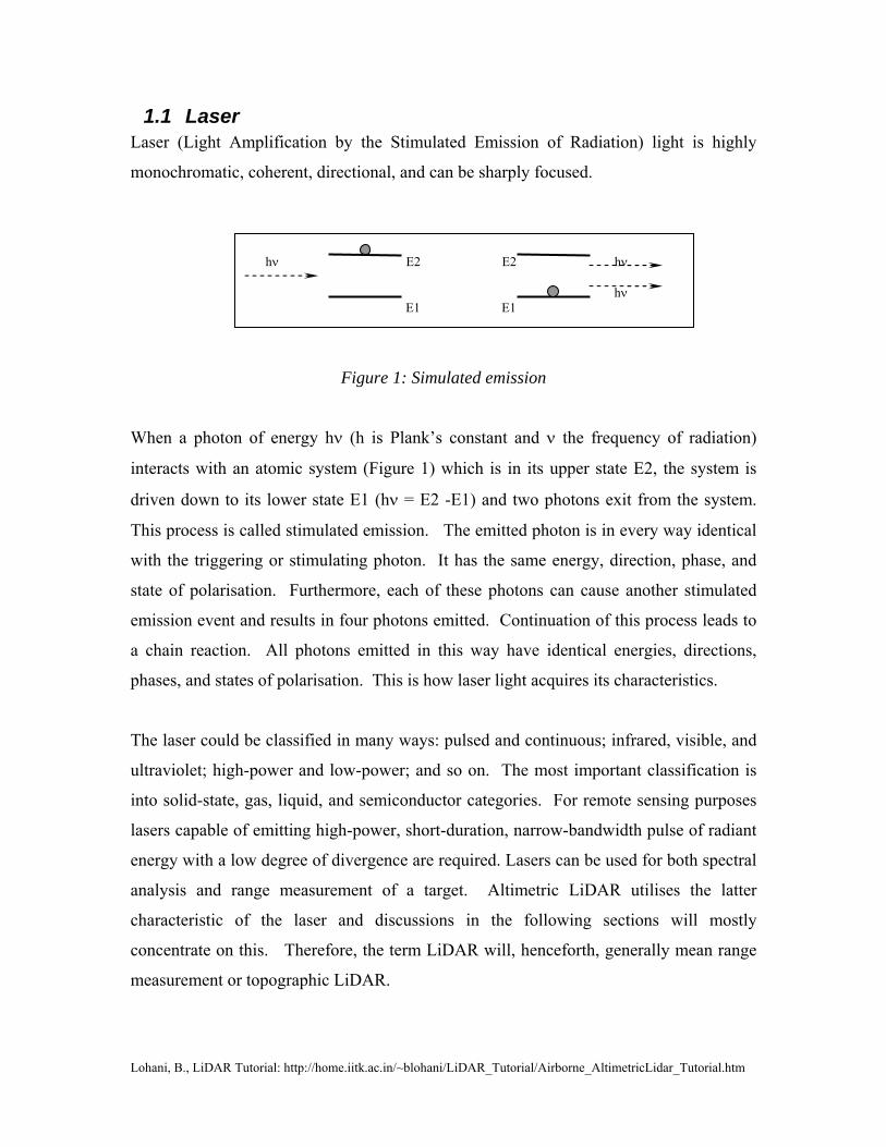
Figure 1: Simulated emission

When a photon of energy hν (h is Plank’s constant and ν the frequency of radiation)

interacts with an atomic system (Figure 1) which is in its upper state E2, the system is

driven down to its lower state E1 (hν = E2 -E1) and two photons exit from the system.

This process is called stimulated emission. The emitted photon is in every way identical

with the triggering or stimulating photon. It has the same energy, direction, phase, and

state of polarisation. Furthermore, each of these photons can cause another stimulated

emission event and results in four photons emitted. Continuation of this process leads to

a chain reaction. All photons emitted in this way have identical energies, directions,

phases, and states of polarisation. This is how laser light acquires its characteristics.

The laser could be classified in many ways: pulsed and continuous; infrared, visible, and

ultraviolet; high-power and low-power; and so on. The most important classification is

into solid-state, gas, liquid, and semiconductor categories. For remote sensing purposes

lasers capable of emitting high-power, short-duration, narrow-bandwidth pulse of radiant

energy with a low degree of divergence are required. Lasers can be used for both spectral

analysis and range measurement of a target. Altimetric LiDAR utilises the latter

characteristic of the laser and discussions in the following sections will mostly

concentrate on this. Therefore, the term LiDAR will, henceforth, generally mean range

measurement or topographic LiDAR.

hν E2 E2 hν hν E1 E1


1.2 Principle of LiDAR The principle of LiDAR is similar to Electronic Distance Measuring Instrument (EDMI),

where a laser (pulse or continuous wave) is fired from a transmitter and the reflected

energy is captured (Figure 2). Using the time of travel (ToT) of this laser the distance

between the transmitter and reflector is determined. The reflector could be natural

objects or an artificial reflector like prism. In case of ranging LiDAR this distance is one

of the primary measurement which with integration with other measurements also

provides the coordinates of the reflector. This is shown in the following paragraphs.

Figure 2 Principle of range measurement using laser

1.2.1 Topographic LiDAR

The Figure 3 shows the various sensors and scanning mechanism involved in LiDAR

data collection. The basic concepts of airborne LiDAR mapping are simple. A pulsed

laser is optically coupled to a beam director which scans the laser pulses over a swath of

terrain, usually centred on, and co-linear with, the flight path of the aircraft in which the

system is mounted, the scan direction being orthogonal to the flight path. The round trip

travel times of the laser pulses from the aircraft to the ground are measured with a precise

interval timer and the time intervals are converted into range measurements knowing the

velocity of light. The position of the aircraft at the epoch of each measurement is

determined by a phase difference kinematic GPS. Rotational positions of the beam

director are combined with aircraft roll, pitch, and heading values determined with an

inertial navigation system (INS), and with the range measurements, to obtain vectors

Transmitter Reflector

Time of travel = TL

Receiver


LASER SCANNER

Z

Y

X

GPS

Z

Y X

GPS

Z

Y

X

INS

GPS

from the aircraft to the ground points. When these vectors are added to the aircraft

locations they yield accurate coordinates of points on the surface of the terrain.

Figure 3: Principle of topographic LiDAR

The principle of using laser for range measurement was known since late 1960s. At the

same time people begun thinking about the use of airborne laser for measurement of

ground coordinates. However, this could not be realized till late 1980s as determination

of location of airborne laser sensor, which is a primary requirement, was not possible.

The operationalization of GPS solved this problem. This is among the important reasons

that why the laser mapping from airborne platform could not be realized before.

The LiDAR technology is known by several names in literature and industry. One may

regularly come across the names like Laser altimetry, Laser range finder, Laser radar,

Laser mapper and Airborne altimetric LiDAR. The term Airborne altimetric LiDAR (or

Simply LiDAR) is the most accepted name for this technology.

The process of computation of ground coordinates is shown in the flow diagram ( Figure 4)


Figure 4: Flow diagram showing various sensors employed in LiDAR instrument and the computation steps

1.2.2 Bathymetric LiDAR Most of the initial uses of LiDAR were for measuring water depth. Depending upon the

clarity of the water LiDAR can measure depths from 0.9m to 40m with a vertical

accuracy of ±15cm and horizontal accuracy of ±2.5m. As shown in Figure 5 a laser

pulse is transmitted to the water surface where, through Fresnel reflection, a portion of

the energy is returned to the airborne optical receiver, while the remainder of the pulse

continues through the water column to the bottom and is subsequently reflected back to

the receiver. The elapsed time between the received surface and bottom pulses allows

determination of the water depth. The maximum depth penetration for a given laser

system is obviously a function of water clarity and bottom reflection. Water turbidity

plays the most significant role among those parameters. It has been noted that water

LiDAR System

Laser Range Scan mirror position Signal strength (Transmit and receive)

Inertial navigation system Pitch Roll Heading

Range calibration (from ground data)

LiDAR to aircraft mounting parameters

Range data Processing software

Global positioning system on aircraft

Global positioning system on ground

Aircraft trajectory

Raw ground coordinates (x, y, z)


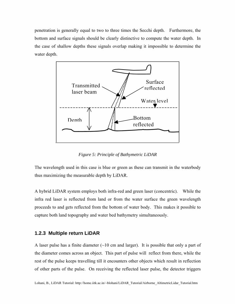
penetration is generally equal to two to three times the Secchi depth. Furthermore, the

bottom and surface signals should be clearly distinctive to compute the water depth. In

the case of shallow depths these signals overlap making it impossible to determine the

water depth.

Figure 5: Principle of Bathymetric LiDAR

The wavelength used in this case is blue or green as these can transmit in the waterbody

thus maximizing the measurable depth by LiDAR.

A hybrid LiDAR system employs both infra-red and green laser (concentric). While the

infra red laser is reflected from land or from the water surface the green wavelength

proceeds to and gets reflected from the bottom of water body. This makes it possible to

capture both land topography and water bed bathymetry simultaneously.

1.2.3 Multiple return LiDAR A laser pulse has a finite diameter (~10 cm and larger). It is possible that only a part of

the diameter comes across an object. This part of pulse will reflect from there, while the

rest of the pulse keeps travelling till it encounters other objects which result in reflection

of other parts of the pulse. On receiving the reflected laser pulse, the detector triggers

Transmittedlaser beam

Surfacereflected

Depth

Water level

Bottomreflected


when the in-coming pulse reaches a set threshold, thus measuring the time-of-flight. The

sampling of the received laser pulse can be carried out in different ways- sampling for the

most significant return, sampling for the first and last significant return, or sampling all

returns which are above threshold at different stages of the reflected laser waveform.

Accordingly, the range is measured to each of those points wherefrom a return occurred

to yield their coordinates.

Figure 6: Example of multiple returns from a tree

In the figure shown above the first return is the most significant return. In case of

capturing of only most significant return the coordinate of the corresponding point (here

the top of tree) only will be computed. Capturing of first and last returns as shown above

will result in determination of the height of the tree. It is important to note that last return

will not always from the ground. In case of a laser pulse hitting a thick branch on its way

to ground the pulse will not reach ground thus no last return from ground. The last return

will be from the branch which reflected entire laser pulse. Commercially available

sensors at present support up to 4 returns from each fired laser pulse and provide the

option to choose among first, first and last and all 4 returns data.

First return

Second return

Third return

Fourth return

Last return

Time

Amplitude


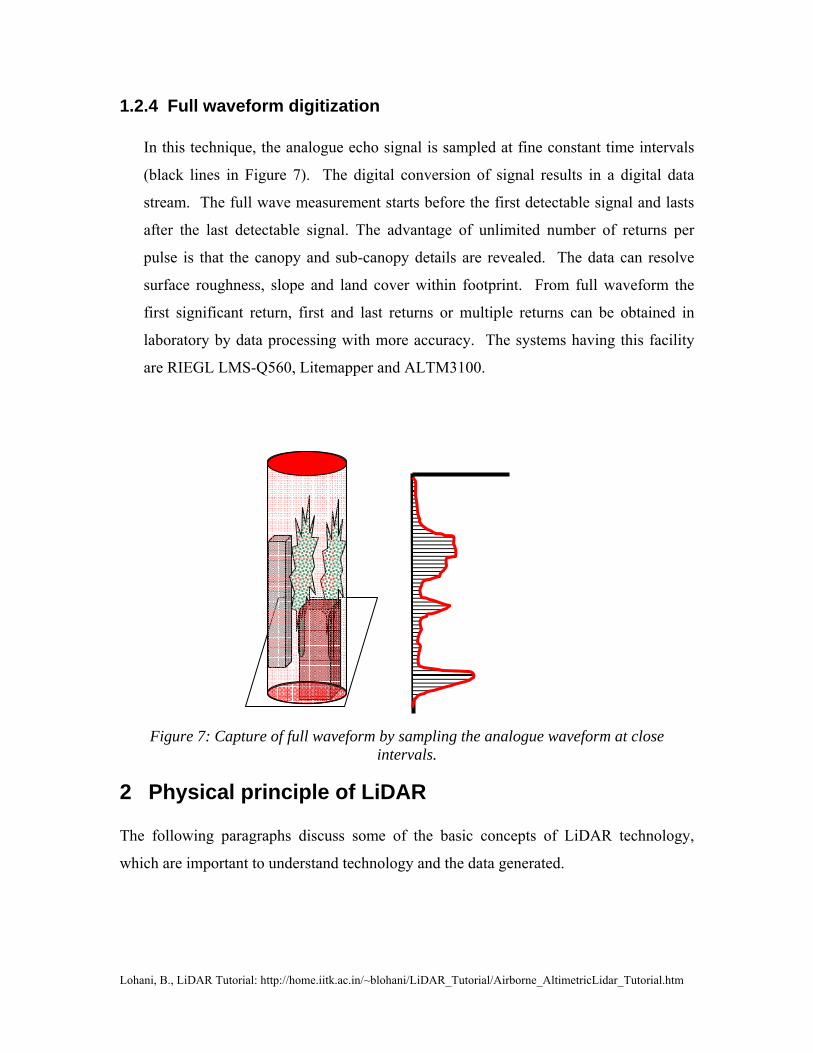
1.2.4 Full waveform digitization

In this technique, the analogue echo signal is sampled at fine constant time intervals

(black lines in Figure 7). The digital conversion of signal results in a digital data

stream. The full wave measurement starts before the first detectable signal and lasts

after the last detectable signal. The advantage of unlimited number of returns per

pulse is that the canopy and sub-canopy details are revealed. The data can resolve

surface roughness, slope and land cover within footprint. From full waveform the

first significant return, first and last returns or multiple returns can be obtained in

laboratory by data processing with more accuracy. The systems having this facility

are RIEGL LMS-Q560, Litemapper and ALTM3100.

Figure 7: Capture of full waveform by sampling the analogue waveform at close

intervals.

2 Physical principle of LiDAR The following paragraphs discuss some of the basic concepts of LiDAR technology,

which are important to understand technology and the data generated.


2.1 Types of range measurement

2.1.1 Continuous wave ranging In this case a continuous beam of Electromagnetic Radiation (EMR) (light here) is used

to measure the distance between transmitter and reflector. This is realized through the

measurement of phase difference between transmitted and received wave. As shown in

Figure 8, the time of travel can be written as:

2LT nT Tϕπ

= +

Where n is the total number of full wavelengths, T is time taken by light to travel equal to

one wavelength and φ is the phase difference. The only unknown in above is n which is

determined using the techniques like decade modulation. So range is given by:

2LTR c=

Figure 8 Continuous wave for phase difference measurement

0

4 4

4

For ncRange R Tcf

cso Rf

ϕ ϕπ πϕ

π

=

= =

ΔΔ =

Transmitter Reflector Time of travel = TL

Receiver


The above shows that the range resolution depends upon the resolution of phase

difference measurement and as well on the wavelength used. The advantage of CW

measurement is that highly accurate measurements can be realised (as the accuracy of

measurement is dependent upon the shortest wavelength used). However, it is difficult to

generate continuous wave of high energy thus limiting the range of operation of these

instruments. The slant range in case of airborne LiDAR is large thus the CW principle of

ToT measurement is generally not used in these sensors.

The maximum range that can be measured by the CW LiDAR depends on the longest

wavelength used, as shown below:

maxmax

maxmax

24 4

2

cRf

So R

ϕ π λπ π

λ

= =

=

2.1.2 Pulse ranging As shown in Figure 9 the time of travel in pulse ranging is measured between the leading

edges of transmitted and received pulse. The range measured is given by:

2LTR c=

Further, the range resolution and maximum range are given by:

max max2 2L Lc cR T and R TΔ = Δ =

In case of pulse ranging the resolution of range measurement depends only on the

resolution of ToT measurement, which is limited by the precision of the clock on the

sensor. The maximum range that can be measured in pulse ranging depends upon the


maximum time that can be measured, as shown above. However, in practice the

maximum range that can be measured depends upon energy of the laser pulse. The

received signal should be of sufficient strength to be distinguished from the noise for

detection. This in turn depends upon the divergence, atmosphere, reflectivity of target

and detector sensitivity. In addition, the Rmax also depends upon the pulse firing rate

(PFR), i.e. number of pulses being fired in one second, which will be understood in later

paragraphs.

Figure 9: Time of travel measurement between transmitted and return pulse

It is clear from the above discussion that in airborne LiDAR pulse ranging is mostly

employed. The discussion in rest of this document will thus be about pulse ranging only.

2.2 Laser pulse and nomenclature Laser pulses are generated using the diode pumped solid state lasers, e.g. Ny-Yag laser.

A typical laser pulse can be considered Gaussian in its amplitude distribution in both

transverse and longitudinal directions. Figure 10 shows schematic of one such pulse.

Here trise is the time taken by pulse to reach 90% amplitude from 10% amplitude. Pulse

Transmitter Reflector

Receiver

Time

Time of travel = TL

Am

plitu

de

Transmitted pulse

Received pulse


width is defined as tp, which is the duration between 50% amplitudes in leading and

trailing edges of the pulse.

Figure 10: A Gaussian pulse

2.3 Time of Travel (ToT) measuring methods In the example of Figure 9 the transmitted and received pulse were assumed as the step

pulses and ToT is measured with the well defined point on leading edges. However, in

actual practice the transmitted pulse is Gaussian while the shape of return pulse depends

upon the geometry, reflectivity and surface roughness with the laser footprint ( a laser

footprint is the area on ground which is illuminated by the laser pulse, due to its

divergence and a finite size of the transmission aperture) on ground. Therefore, if is quite

common that the return pulse may have a distorted, multimodal and depleted shape. To

measure the ToT on this one needs to define a point corresponding to a point on the

transmitted pulse. The following methods are used for this purpose.

2.3.1 Constant fraction method The ToT is measured w.r.t. a specific point on leading edge. The time counter is

started by transmit pulse. Time counter stops when the voltage reaches a pre-

Am

plit

ude

tp

100%

50%

10%

90%

Time

trise


specified value for received pulse. This is measured on more steep leading

edge/rising slope. In case of ideal return there will be no error in ToT measurment.

However, due to different amplitude returns (different slopes of leading edges of

return pulses) from the targets with different reflectivity and topology different ToT

will be measured notwithstanding the targets being at same distance from the sensor.

This is called range walk. Figure 11 shows how the ToT is measured for an ideal

return (middle line) and for returns from targets of different reflectivity. The ToT

measured for ideal return is without error, however, the range walk is introduced for

other returns (lower line).

Figure 11: Time measurement by constant fraction

The error due to range walk needs to be eliminated. Some approaches for this will be

discussed in following paragraphs.

Th


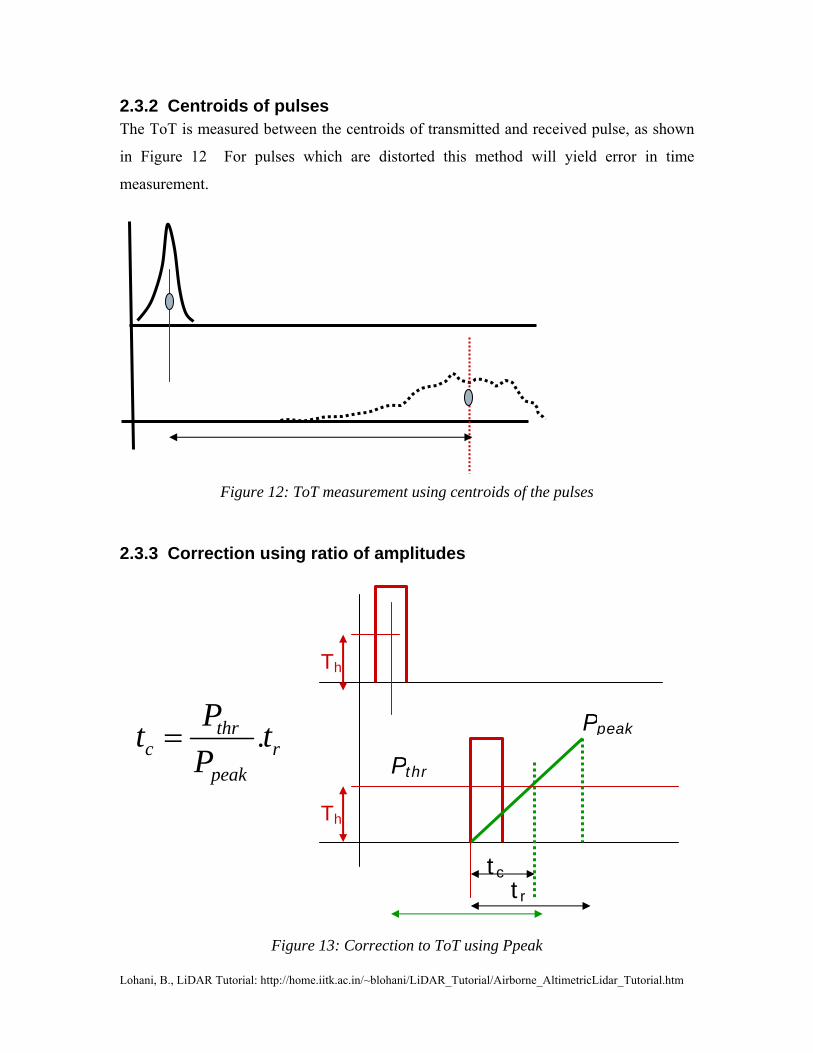
2.3.2 Centroids of pulses The ToT is measured between the centroids of transmitted and received pulse, as shown

in Figure 12 For pulses which are distorted this method will yield error in time

measurement.

Figure 12: ToT measurement using centroids of the pulses

2.3.3 Correction using ratio of amplitudes

Figure 13: Correction to ToT using Ppeak

Th

Th

tc

Ppeak

Pthr

tr

.thrc r

peak

Pt tP

=


In this method correction to measured time is applied using the power of returned signal.

The basic idea is to bring the time of travel to the level of step pulse, i.e., where for step

pulse is being measured. The correction to be applied in measured time is given by tc as

shown in Figure 13:

2.3.4 Correction using calibration

Figure 14: Range calibration curve(Modified after Ridgway et al, 1997)

This method aims at applying correction for range walk in range or in ToT measured by

constant fraction method, as discussed above. The calibration data (time or range

measured vs. amplitude of returned energy) are collected at a test site. The actual

distance between sensor and target is known which is used to determine correction to

time or range. The plot of correction versus amplitude of return pulse (as shown in

Figure 14) is the calibration curve. The timings recorded by sensor are corrected by

using the calibration curve for the measured values of return amplitude.

Ran

ge

Corr

ection c

m

Amplitude of waveform peak (0 – 255)


2.4 Requirement of the laser for altimetric LiDAR Altimetric LiDAR primarily uses the range measured by the laser ranger. To realise

accurate and long range measurement the laser pulse should have the following

characteristics:

• High power: So reflectance is available at receiver

• Short pulse length: Less uncertainty in time measurement

• High collimation: Less uncertainty due to smaller footprint

• Narrow optical spectrum: Small bandpass filter to reduce noise

• Eye safety: The lasers are more dangerous as wavelength reduces

• Spectral reflectivity of laser from terrain features: So reflectance (signal) is

available.

2.5 LiDAR power and pulse firing rate For a pulse with Ppeak power and tp pulse width the energy in one pulse can be given by

. The total energy spent in one second will be , where F is the pulse

firing rate (PFR). Thus the average power that is being spent per second is

. This leads to the conclusion that, for a given power and pulse width the PFR is

inversely related to peak power of pulse. With the increase in altitude (range) one needs

the pulses with higher peak power. For same value of Pav and tp, thus with increase in

altitude the PFR will reduce. This is reflected in the specifications of various sensors.

2.6 Geolocation of LiDAR footprint In LiDAR surveying the following basic measurements are obtained for each laser pulse

fired:

• Laser range by measuring ToT of a pulse

• Laser scan angle

• Aircraft roll, pitch and yaw

• Aircraft acceleration in three directions

peak pE P t= avP EF=

av peak pP P t F=


• GPS antenna coordinates

Geo-location means how to determine the coordinates of laser footprint in WGS-84

reference system by combining the aforesaid basic measurements.

As seen in Figure 15, a LiDAR system consists of three main sensors, viz. LiDAR

scanner, INS and GPS. These systems operate at their respective frequencies. The laser

range vector which is fired at an scan angle η in the reference frame of laser instrument

will need to be finally transformed the earth cantered WGS-84 system for realising the

geolocation of the laser footprint. This transformation is carried through various

rotations and transformatios as shown below. First it is important to understand the

various coordinate systems involved in this process and their relationships.

2.6.1 Reference systems Instrument Reference system:

This is at centre of laser output mirror with Z axis along path of laser beam at centre of

laser swath and X in the direction of aircraft nose while Y is as per right hand coordinate

system. This is shown by black colour in Figure 15. This reference system will move

and rotate with aircraft.

Scanning reference system:

The red lines in Figure 15 indicate the laser pulse and corresponding time-variable axis

system with z being in the direction of laser pulse travel. The x axis is coincident with

instrument reference X axis. The direction of z axis is fixed as per the instantaneous scan

angle η.

INS reference system (Body) :

INS is aligned initially to local gravity and True North when switched on. It works by

detecting rotation of earth and gravity. The origin of INS reference system is at INS with

X, Y, Z defined as local roll, pitch, and yaw axes of airplane. Here X is along nose and

Y along right wing of aircraft in a RH coordinate system. The INS gives the roll, pitch,

and yaw values w.r.t. to the initially aligned system at any moment.

The above three reference systems are related to each other. Blue dotted lines are INS

body axis with origin at instrument while black lines are instrument axis. These differ


due to mounting errors which are referred to as mounting biases in roll, pitch, and yaw

and determined by calibration process. They also differ due to translation between INS

and the laser head. The red lines indicate the laser pulse and corresponding time-variable

axis system with z being in the direction of laser pulse travel. This is due to scan angle η.

This reference system is related to instrument reference system with rotation angle η.

Earth tangential (ET) reference system

It has its origin at onboard GPS antenna with X axis pointing in the direction of True

north and Z axis pointing towards mass centre of Earth in a right handed system. This is

variable for each shot in flight and can be conceptualized and realized computationally

with the attitude measurements (Figure 16).

ET reference system is related to INS reference system by roll, pitch, and yaw

measurements about X, Y, and Z, respectively, at the time of each shot. ET is also

related to Instrument System by the GPS vector measured in INS reference system.

WGS-84 is related to ET by location of GPS antenna at the time of each laser shot.

2.6.2 Process for geolocation

Range measurement is represented as a vector [0,0,z] in temporary scanning system.

Rotate this vector in instrument reference system using scan angle (η). Further rotate the

vector in INS reference system with origin at instrument using the mounting angle biases

(α0 β0 γ0). Now this vector is translated by GPS vector [dx,dy,dz] measured in INS

reference system. Next step is to rotate the vector to the ET system using roll, pitch, raw

(α β γ). At this stage the vector is in ET system with origin at GPS antenna. Now rotate

the vector in WGS-84 Cartesian system with origin at GPS antenna, using antenna

latitude and longitude (φ, λ), which are measured by GPS. The vector is translated in

Earth-centered WGS-84 system using Cartesian coordinates of antenna (ax, ay , az), as

observed by the GPS. The vector now refers to the Cartesian coordinates of laser

footprint in WGS84, which can be converted in ellipsoidal system. If Rx(θ) is rotation

about x axis by θ angle, T(V) is translation by a vector V, [X’] is final vector in WGS-84


system and φ and λ are latitude and longitude of GPS antenna at the time of laser shot the

aforesaid steps can be written as:

[ ] 0 0 0, , [0,0, ] ( ) ( ) ( ) ( ) ( , , ) ( ) ( ) ( ) ( ) ( ) ( , , )2x x y z x y z x y z y z x y zx y z z R R R R T d d d R R R R R T a a aπη α β γ α β γ φ λ′ ′ ′ = + −

Figure 15: Relationship between laser scanner, INS and GPS and various reference systems.

Laser

GPS vector [dx,dy,dz] in INS reference system

z y INS

x

η z

x

y

z y

x

zGPS to earth mass centre yGPS

XGPS to True North

GPS Earth tangential reference system


Figure 16: Relationship between ET and WGS-84 system

3 LiDAR sensor and data characteristics

3.1 Available sensors An excellent comparison of various available LiDAR sensors can be found at (Lemmens,

2007) . Sensors vary in their specifications and accordingly are suitable for collecting

data with varied characteristics, as required in different applications. Moreover, each

sensor possesses a large range of parameters in order to arrive at the required data

specification. Some of the most commonly used sensors are ALTM by Optech Canada,

ALS by Leica Geosystems, Toposys by Toposys GmBH, TopEye by Hansa Luftbild and

RIEGL.

X in the direction of prime meridian

Z passing through the True north pole

ET Reference

Laser vector in ET reference system

Laser vector in WGS 84 system

WGS 84 system with origin at GPS antenna


3.2 LiDAR Scanning pattern Scanning pattern on ground depends primarily on the LiDAR sensors which scan the

ground in different modes. The pattern also gets affected by the nature of terrain and the

perturbations (attitude and acceleration) in flight trajectory. A few common types are

described below:

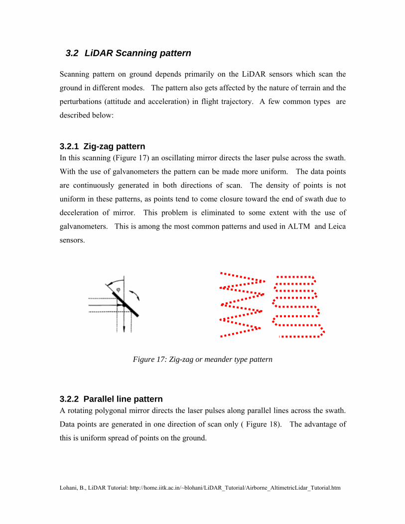
3.2.1 Zig-zag pattern In this scanning (Figure 17) an oscillating mirror directs the laser pulse across the swath.

With the use of galvanometers the pattern can be made more uniform. The data points

are continuously generated in both directions of scan. The density of points is not

uniform in these patterns, as points tend to come closure toward the end of swath due to

deceleration of mirror. This problem is eliminated to some extent with the use of

galvanometers. This is among the most common patterns and used in ALTM and Leica

sensors.

Figure 17: Zig-zag or meander type pattern

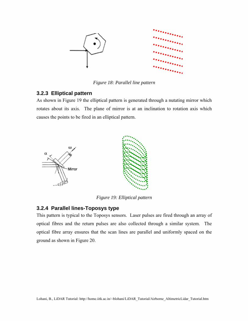
3.2.2 Parallel line pattern A rotating polygonal mirror directs the laser pulses along parallel lines across the swath.

Data points are generated in one direction of scan only ( Figure 18). The advantage of

this is uniform spread of points on the ground.


Figure 18: Parallel line pattern

3.2.3 Elliptical pattern As shown in Figure 19 the elliptical pattern is generated through a nutating mirror which

rotates about its axis. The plane of mirror is at an inclination to rotation axis which

causes the points to be fired in an elliptical pattern.

Figure 19: Elliptical pattern

3.2.4 Parallel lines-Toposys type This pattern is typical to the Toposys sensors. Laser pulses are fired through an array of

optical fibres and the return pulses are also collected through a similar system. The

optical fibre array ensures that the scan lines are parallel and uniformly spaced on the

ground as shown in Figure 20.


Figure 20: Parallel line pattern (Courtesy Toposys)

3.3 Data density Data density is an important parameter in LiDAR survey. While a dense data captures

the terrain better and helps in information extraction the time and resource requirement is

high. The data density is decided depending the application for which the data are being

collected. The data density mainly depends upon the parameters of sensor and platform

e.g., flying height, velocity, scan angle, scan frequency, pulse firing rate, scanning

pattern, acceleration and attitude variation of platform. Additionally, it also depends

upon the ground geometry and reflectivity.

Figure 21: Scan definitions

Depending the sensor a scan could be of any of the two types as shown in Figure 21.

Considering the scan frequency is fsc the number of data points in one scan will be:

sc

FNf

=


If the platform is at an altitude of H and scan angle is θ the swath S is given by:

2 tan2

S H θ⎛ ⎞= ⎜ ⎟⎝ ⎠

Thus the data density (points per unit length) across the track (i.e. in the direction of scan)

is given by :

2

s

s

Nd for unidirectional scanS

andNd for bidirectional scanS

=

=

The data density along the track is variable for zig-zag scan and uniform for parallel line

pattern. The maximum separation is given by:

maxavdf

=

Another approach to represent data density is as number of points in unit area. In this

case the data density can be given by:

FdvS

=

where v is the velocity of airborne platform and vS is the area covered in one second

while F is the number data points generated in one second. In above it is assumed all

fired pulses will result in a measurement.

3.4 Example LiDAR data An example LiDAR data is shown below for first and last return. LiDAR data are available either in ASCII format or in the standard .LAS format.

X Y Z R X Y Z R512548.36 5403119.37 314.29 10 512548.20 5403120.90 303.43 28 512548.39 5403120.61 313.73 20 512548.24 5403122.08 303.45 44 512548.36 5403122.39 308.73 48 512548.28 5403123.17 303.35 66 512548.40 5403123.05 310.07 26 512548.31 5403124.02 303.45 172 512548.40 5403123.92 308.46 0 512548.33 5403124.67 303.40 203 512548.34 5403125.09 303.43 290 512548.34 5403125.09 303.43 290 512548.35 5403125.41 303.47 319 512548.35 5403125.41 303.47 319 512548.35 5403125.74 303.47 319 512548.35 5403125.74 303.41 319 512548.36 5403125.95 303.46 290 512548.35 5403125.96 303.43 290


4 LiDAR error sources The various sensor components fitted in the LiDAR instrument possess different

precision. For example, in a typical sensor the range accuracy is 1-5 cm, the GPS

accuracy 2-5 cm, scan angle measuring accuracy is 0.01°, INS accuracy for pitch/roll is <

0.005° and for heading is < 0.008° with the beam divergence being 0.25 to 5 mrad.

However, the final vertical and horizontal accuracies that are achieved in the data are of

order of 5 to 15 cm and 15-50 cm at one sigma. The final data accuracy is affected by

several sources in the process of LiDAR data capture. A few important sources are listed

below:

• Error due to sensor position due to error in GPS, INS and GPS-INS integration.

• Error due to angles of laser travel as the laser instrument is not perfectly aligned

with the aircraft’s roll, pitch and yaw axis. There may be differential shaking of

laser scanner and INS. Further, the measurement of scanner angle may have

error.

• The vector from GPS antenna to instrument in INS reference system is required in

the geolocation process. This vector is observed physically and may have error in

its observation. This could be variable from flight to flight and also within the

beginning and end of the flight. This should be observed before and after the

flight.

• There may be error in the laser range measured due to time measurement error,

wrong atmospheric correction and ambiguities in target surface which results in

range walk.

• Error is also introduced in LiDAR data due to complexity in object space, e.g.,

sloping surfaces leads to more uncertainty in X, Y and Z coordinates. Further,

the accuracy of laser range varies with different types of terrain covers.

• The divergence of laser results in a finite diameter footprint instead of a single

point on the ground thus leading to uncertainty in coordinates. For example, if

sensor diameter Ds = 0.1 cm; divergence= 0.25 mrad; and flying height 1000m,

the size of footprint on the ground is Di= 25 cm. Varying reflective and

geometric properties within footprint also lead to uncertainty in the coordinate.


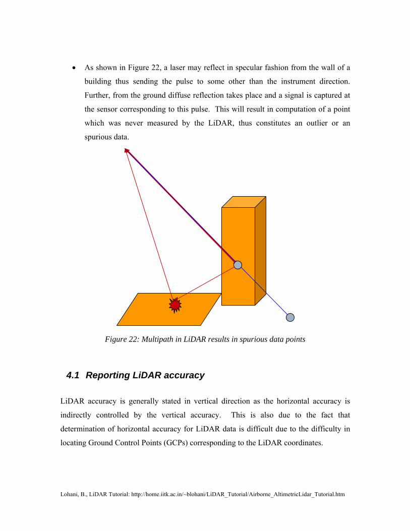
• As shown in Figure 22, a laser may reflect in specular fashion from the wall of a

building thus sending the pulse to some other than the instrument direction.

Further, from the ground diffuse reflection takes place and a signal is captured at

the sensor corresponding to this pulse. This will result in computation of a point

which was never measured by the LiDAR, thus constitutes an outlier or an

spurious data.

Figure 22: Multipath in LiDAR results in spurious data points

4.1 Reporting LiDAR accuracy

LiDAR accuracy is generally stated in vertical direction as the horizontal accuracy is

indirectly controlled by the vertical accuracy. This is also due to the fact that

determination of horizontal accuracy for LiDAR data is difficult due to the difficulty in

locating Ground Control Points (GCPs) corresponding to the LiDAR coordinates.


The vertical accuracy is determined by comparing the Z coordinates of data with the truth

elevations of a reference (which is generally a flat surface). The accuracy is stated as

RMSE and given by:

LiDAR accuracy is reported generally as 1.96 RMSEz. This accuracy is called

fundamental vertical accuracy when the RMSE is determined for a flat, non-obtrusive

and good reflecting surface. While the accuracy should also be stated for other types of

surfaces, which are called supplemental and consolidated vertical accuracies.

5 Application of airborne altimetric LiDAR Application areas for LiDAR can be divided in three main categories (1) Competing-

where LiDAR is competing with existing topographic data collection methods; (2)

Complementing- where LiDAR is complementing the existing topographic data

collection methods and (3) New applications- where LiDAR data are finding applications

in those areas which were not possible hitherto with the conventional data collection

methods.

The following is a brief list of the areas where LiDAR data are being applied:

5.1 Floods • Improving flood forecast models and flood hazard zoning operations with the use

of more accurate topographic data.

• The information provided by LiDAR about the above ground objects can help in

the determination of the friction coefficient on flood plains locally. This improves

the performance of flood model.

• Topographic data input to GIS based relief, rescue, and flood simulation

operations.

5.2 Coastal applications • Coastal engineering works, flood management and erosion monitoring

2( ) ( )( ( )data i check i

z

Z ZRMSE

n∑ −

=


• LiDAR is especially useful for coastal areas as these are generally inaccessible

and featureless terrain. While being inaccessible prohibits land surveying or GPS

survey the featureless terrain restricts use of photogrammetry due to absence of

GCPs.

• The coastal landform mapping, e.g., mapping of tidal channels and other

morphological features is possible by employing LiDAR data for change

detection studies.

5.3 Bathymetric applications • For mapping river and coastal navigation channels and river and coastal bed

topography

5.4 Glacier and Avalanche • Mapping glacial topography

• Attempts have been made for measuring ice velocities by comparing the relative

position of glacial landforms on LiDAR data of two times.

• Risk assessment for avalanche by monitoring snow accumulation by LiDAR.

5.5 Landslides • Monitoring landslide prone zones. Continuous monitoring will lead to prediction

of possible slope failures.

5.6 Forest mapping • LiDAR pulses are capable of passing through the small gaps in forest canopy.

Thus data points will be available under the canopy of a tree. Algorithms are

available which can separate the data points on trees and on the ground, thus

producing a DEM of the forest floor (Figure 23). The forest floor DEM has

applications in forest fire hazard zoning and disaster management

• As LiDAR data points are spread all over the canopy, models are being developed

for estimation of biomass volume using LiDAR data.

• The information about percentage of points which penetrate the canopy of a tree

can be related to the Leave Area Index (LAI)


Figure 23: LiDAR data of forest (top) and corresponding forest floor DEM

(below)(Courtesy Geolas)

5.7 Urban applications LiDAR data can be used for generating the

maps of urban areas at large scale. LiDAR

facilitates identification of buildings from the

point cloud of data points, which are

important for mapping, revenue estimation,

and change detection studies. Drainage

planning in urban areas needs accurate

topographic data which are not possible to be

generated in busy streets using conventional

methods. The ability of LiDAR to collect data

even in narrow and shadowy lanes in cities

makes is ideal for this purpose. Accurate,

dense and fast collection of topographic data

can prove useful for variety of other GIS

applications in urban areas, e.g. visualization,

emergency route planning, etc.

Figure 24: LiDAR data for a hotel (Courtesy Geolas)


5.8 Cellular network planning LiDAR collects details of building outlines, ground cover and other obstructions. This

can be used to carry out accurate analysis for determining line of sight and view shed for

proposed cellular antenna network with the purpose of raising an optimal network in

terms of cost and coverage.

5.9 Mining • To estimate ore volumes

• Subsidence monitoring

• Planning mining operations

5.10 Corridor mapping This is among the most interesting applications of LiDAR data. A helicopter bound

LiDAR sensor is generally used for mapping of corridor by flying at lower altitude for

collecting accurate and dense data

of corridors. A corridor may be

highway, railway or oil and gas

pipe line. The data are useful in

planning the corridor and during

execution of work and later for

monitoring the deflections,

possible areas of repair etc. High

density of data facilitates

generation of a record of the assets

of the corridor.

Figure 25: A highway corridor captured using LiDAR data

5.11 Transmission line mapping This is an area which was not possible with conventional topographic data techniques and

where the LiDAR data are being used most. The LiDAR pulses get reflected highly from


the wires of transmission lines thus generating a coordinate at the wire. Multiple returns

produce data for different story of wires. In addition, LiDAR also captures the natural

and artificial objects under and around the transmission lines (Figure 26). This

information is extremely useful for knowing tower locations, structural quality of towers,

determining catenary models of lines, carrying out vegetative critical distance analysis

and for carrying out repair and planning work in a transmission line corridor Figure 26.

Figure 26: Transverse section of a transmission line using LiDAR data

There are many more application areas for LiDAR data e.g., Creating realistic 3D

environment for movies, games, and pilot training; Simulation of Hurricane movement

and its effect; Simulation of Air pollution due to an accident or a polluting source;

Transport of vehicular pollution in urban environment; etc. Basically, all those

application areas where topographic data are fundamental can benefit with LiDAR data.

LiDAR instruments are also being used for extra-terrestrial mapping (e.g. MOLA, LLRI)

6 Advantages of LiDAR technology The other methods of topographic data collection are land surveying, GPS,

inteferrometry, and photogrammetry. LiDAR technology has some advantages in

comparison to these methods, which are being listed below:

Higher accuracy

Vertical accuracy 5-15 cm (1σ) Horizontal accuracy 30-50 cm

Fast acquisition and processing

Acquisition of 1000 km2 in 12 hours. DEM generation of 1000 km2 in 24 hours.


Minimum human dependence

As most of the processes are automatic unlike photogrammetry, GPS or land surveying.

Weather/Light independence

Data collection independent of sun inclination and at night and slightly bad weather.

Canopy penetration

LiDAR pulses can reach beneath the canopy thus generating measurements of points there unlike photogrammetry.

Higher data density

Up to 167,000 pulses per second. More than 24 points per m2 can be measured.

Multiple returns to collect data in 3D.

GCP independence Only a few GCPs are needed to keep reference receiver for the purpose of

DGPS. There is not need of GCPs otherwise. This makes LiDAR ideal for mapping inaccessible and featureless areas.

Additional data

LiDAR also observes the amplitude of back scatter energy thus recording a reflectance value for each data point. This data, though poor spectrally, can be used for classification, as at the wavelength used some features may be discriminated accurately.

Cost

Is has been found by comparative studies that LiDAR data is cheaper in many applications. This is particularly considering the speed, accuracy and density of data.

Reference: Lemmens, M., 2007, Airborne LiDAR Sensor: Product Survey, GIM International, 21(2) Ridgway et al., 1997, Airborne alser altimeter survey of Long Valley California, Geophys, J. Int, 1331, 267-280

airborne altimetric lidar: principle, data collection...

Documents