Math GeosciDOI 10.1007/s11004-015-9599-5

SPECIAL ISSUE

Air Quality Index Revisited from a CompositionalPoint of View

Eusebi Jarauta-Bragulat1 · Carme Hervada-Sala2 ·Juan José Egozcue1

Received: 23 September 2014 / Accepted: 10 May 2015© International Association for Mathematical Geosciences 2015

Abstract The so-calledAir Quality Index (AQI), expresses the quality of atmosphericair. The overall AQI is determined from the AQIs of some reference air pollutants,which are calculated by a transform of the respective concentrations. Concentrationsof air pollutants are compositional data; they are expressed as part of mass of eachpollutant in a total air volume or mass. Therefore, air pollution concentration data,as compositional data, just provide ratio information between concentrations of pol-lutants. Operations involved in the computation of overall AQI are not admissibleoperations in the framework of compositional data analysis, as they destroy the origi-nal ratio information. Consequently, the standard methodology should be reviewed forsuch calculations, taking into account the principles and operations of compositionaldata analysis. The objective of this article is to present a first approach to incorporatecompositional perspective to air quality expression. For this, it is proposed to use abalance log-contrast of concentrations expressed in µg/m3 to define a new kind of airquality indicator. Furthermore, the geometric mean of the concentrations is appliedto obtain a new and simple scale air quality index, avoiding definition of piecewiselinear interpolations used in the standard AQI computation. As an illustrative exam-ple, statistical analysis of atmospheric pollution data series (2004–2013) of the city ofMadrid (Spain) has been carried out.

Keywords Air pollution · Air Quality Index · Compositional data analysis ·Log-contrast · Balance

B Eusebi Jarauta-Bragulateusebi.jarauta@upc.edu

1 Departament de Matemàtica Aplicada III, ETS Enginyers de Camins, Canals i Ports deBarcelona, Universitat Politècnica de Catalunya, Jordi Girona 1-3, C2, 08034 Barcelona, Spain

2 Departament de Física i Enginyeria Nuclear, Escola d’Enginyeria de Terrassa,Universitat Politècnica de Catalunya, Colom 1, TR1, 08222 Terrassa, Spain

123

Math Geosci

1 Introduction

In recent years, air quality has become a social concern due to its consequences onpopulation’s health. Nowadays, there is a clear society demand to live with reasonableenvironmental quality, and one of the most important environmental factors is airquality. According to TheWorld Bank (2013), more than half of the human populationis living in urban areas. In big cities, where there is a large concentration of population,a reasonable good air quality is then required. On top of this, there is a call for timelyand reliable information on air quality, for good data management and measures toprotect the health of population.

In this context, air quality must be defined, measured and expressed in an adequateand comprehensible way. Authorities must undertake a proper air quality manage-ment and people should be able to understand measures taken in order to keep airquality under thresholds. To quantify air quality, some indices have been defined, allrelated to pollutants’ concentration in air. Themost commonly used pollutants for AQIcomputation are ozone (O3), carbon monoxide (CO), sulfur dioxide (SO2), nitrogendioxide (NO2) and suspended particles classified by their maximum diameter (PM2.5,PM10). The most common air quality indices have been analyzed: AQI defined bythe US Environmental Protection Agency (http://www.epa.gov/), the CAQI definedin the European project CITEAIR (van den Elshout et al. 2008) and the revised AQIproposed by Plaia et al. (2013). Plaia and Ruggieri (2011) review air quality indicesand Bishoi et al. (2009) do a comparative study of them. Russo and Soares (2014),after a review of concepts on air pollution, introduced a predictive spatiotemporalmodel. In most cases, the compositional nature of air pollution data is not taken intoaccount neither in the scientific research context nor in the guidelines for environ-mental authorities. This contribution is aimed at giving methodological suggestionson how compositional data principles may be applied in future developments.

Air quality indices are commonly based on air pollutant concentrations and, thus,functions transforming air pollutant concentrations into indexes are required. Most ofair quality index computingmethods use a similar algorithm involving piecewise linearfunctions, which transforms concentrations into normalized indexes. The intervals aredefined by breakpointswhich are chosen to fit both observed and subjectively evaluatedhealth impacts. The piecewise linear function in this case is

AQI(P) = AQIHI − AQILOBPHI − BPLO

(C(P) − BPLO) + AQILO,

BPLO ≤ C(P) < BPHI, (1)

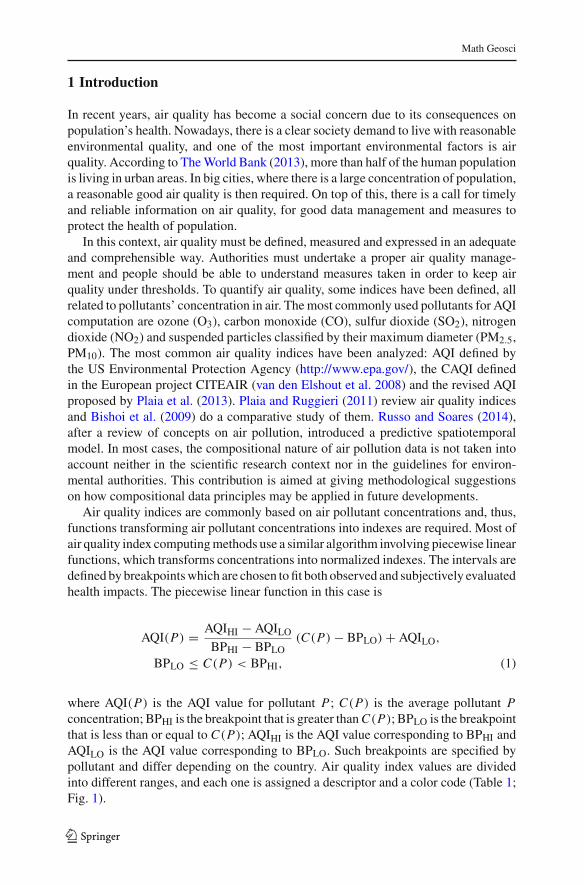
where AQI(P) is the AQI value for pollutant P; C(P) is the average pollutant Pconcentration; BPHI is the breakpoint that is greater thanC(P); BPLO is the breakpointthat is less than or equal to C(P); AQIHI is the AQI value corresponding to BPHI andAQILO is the AQI value corresponding to BPLO. Such breakpoints are specified bypollutant and differ depending on the country. Air quality index values are dividedinto different ranges, and each one is assigned a descriptor and a color code (Table 1;Fig. 1).

123

Math Geosci

Table 1 AQI breakpoints and corresponding color codes

Fig. 1 Piecewise linear function assigning AQI values to concentration of pollutant (µg/m3)

Standardized public health alert protocols are associated with each AQI range. Thepresence of pollutants in air is expressed by their concentration, usually in µg/m3 andsometimes in parts per million of mass (ppm) or in parts per billion of mass (ppb).Daily andmonthly averages of concentrations are carried out using the arithmeticmeanof the corresponding measured values for each element and over the correspondingperiod of time. These average values are used to assign the corresponding AQI valuesfor each pollutant. The final air quality report usually contains the maximum AQIof different air pollutants, the average of the two greatest ones and the arithmeticmean (average) of all AQIs, the so-called overall AQI. As a comment, note that AQIindexes express the degree of pollution and, strictly speaking, not the quality of theair. Certainly, the larger the AQI, which means the larger the pollution, the worse doesthe air quality get. Nevertheless, the term “quality” is maintained for the standard airquality indices.

123

Math Geosci

Concentrations of air pollutants are compositional data. They describe the parts inwhich the whole amount (volume or mass) of air is decomposed. This means that theinformation provided by this kind of data comes from the ratios between differentparts. The analysis of compositional data must be done according to some principles(Aitchison 1986; Aitchison and Egozcue 2005; Egozcue 2009). For instance, scaleinvariance principle requires that a change of units in concentrations, for example,from proportions to ppm, does not change the result of the analysis; subcompositionalcoherence principle preconizes that results obtained from the analysis of a compositioncannot be contradictory with those obtained from the analysis of a subcomposition.Violation of some of these principles may lead to inconsistent results. Pearson (1897),one of the founders of modern statistics, who pointed out the spurious correlationphenomenon, did the very first reference of such problems.

In the eighties, Aitchison (1986) put forward the so-called log-ratio approach, defin-ing suitable techniques to deal with compositional data. From then on, there have beensignificant advances in the formal aspects of the analysis that allow greater system-atization of his methods. To sum it up, statistical analysis of compositional data canbe stated as a three-step process: (1) transforming data in log-ratio coordinates; (2)performing statistical analysis of those coordinates as real variables; (3) interpretingthe results on the coordinates or back transforming them into compositional data.However, the usage of this process is not as widespread as it deserves (Egozcue andPawlowsky-Glahn 2011b).

The main goal of this paper is to contribute to improve analysis, interpretationand management of air quality using compositional data techniques. Particularly, theinterest is focused on the formulation of a new air quality index that satisfies therequisites of compositional data analysis. Other advanced aspects of the analysis ofair quality are out of the scope of this contribution. For instance, evolution in spaceusing geostatistics (Russo and Soares 2014) or applying differential equations in thesimplex (Egozcue and Jarauta-Bragulat 2014). Further research should be necessaryto get a complete, coherent and comprehensive air quality approach, considering theperspective of compositional data analysis.

2 Compositional Approach

The methodological aspects will be demonstrated using a data set granted by theAyuntamiento de Madrid (Spain). The monthly mean concentrations of air pollutantsO3, PM2.5, PM10, CO, SO2, NO2 are taken from the years 2004 to 2013, constitutinga sample of n = 117 monthly data points.

The first step in the analysis was to compare averages of pollutant concentrationsand averages of corresponding AQIs. Note that the NO2 data values are removed forthis comparison because this pollutant, for low concentrations, gives null values of thecorresponding AQI. As the functions relating concentrations to AQIs are piecewiselinear functions of the pollutant concentrations (Eq. 1), it is reasonable to expect a goodcorrelation between the arithmetic average of pollutant concentrations and arithmeticaverage of AQIs, which is the overall AQI.

123

Math Geosci

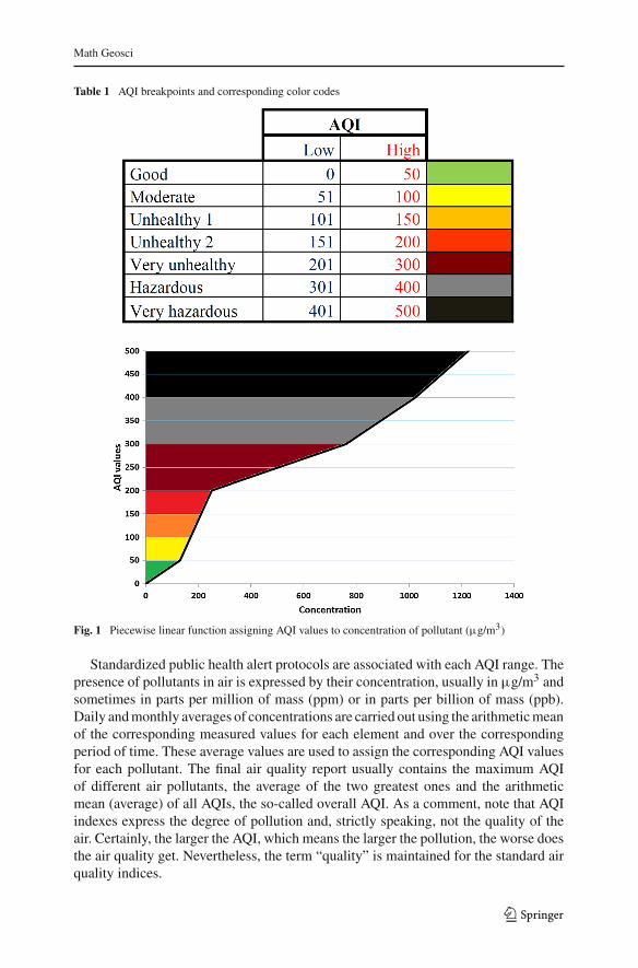
Figure 2a shows time evolution of the arithmetic mean of pollutant concentrationsand the arithmetic mean of pollutant AQIs. Figure 2b shows the scatterplot of pollutantconcentration arithmetic average versus AQI arithmetic average, with the correlationcoefficient for these two variables being 0.579, which is a value smaller than expected.Moreover, the shape of the two curves in Fig. 2a is different.

Fig. 2 a Pollutant concentration (µg/m3) arithmetic mean (green) and AQI arithmetic mean (purple) as afunction of time (months). b Scatterplot of pollutant concentration (µg/m3) arithmetic mean versus AQIarithmetic mean. Data set Madrid 2004–2013

123

Math Geosci

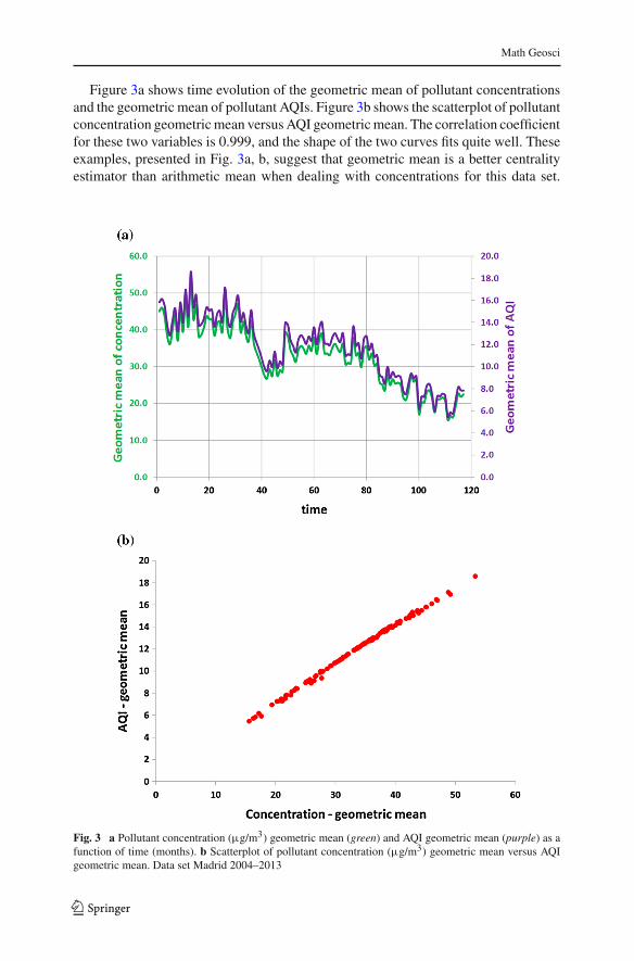
Figure 3a shows time evolution of the geometric mean of pollutant concentrationsand the geometric mean of pollutant AQIs. Figure 3b shows the scatterplot of pollutantconcentration geometricmean versusAQI geometricmean. The correlation coefficientfor these two variables is 0.999, and the shape of the two curves fits quite well. Theseexamples, presented in Fig. 3a, b, suggest that geometric mean is a better centralityestimator than arithmetic mean when dealing with concentrations for this data set.

Fig. 3 a Pollutant concentration (µg/m3) geometric mean (green) and AQI geometric mean (purple) as afunction of time (months). b Scatterplot of pollutant concentration (µg/m3) geometric mean versus AQIgeometric mean. Data set Madrid 2004–2013

123

Math Geosci

Table 2 Correlation matrices of air pollutants in Madrid showing the effect of spurious correlation

(a) When concentrations of pollutants are expressed in ppb of mass; (b) when concentrations of pollutantsare expressed of proportions in mass in the subcomposition O3, PM2.5, PM10, CO, SO2

This is in accordance with well-known facts in compositional data analysis (Aitchison1986; Aitchison and Egozcue 2005).

The concentrations of air pollutants constitute a compositional vector, a composi-tion for short. Compositions represent parts of a whole, which, in this case, are totalmicrograms in a cubic meter of air. The information conveyed by a composition issummarized in the ratios between different parts. Therefore, when multiplying a com-position by a constant, information does not change and the two vectors are equivalentas compositions. For instance, expressing air pollutants in µg/m3 is equivalent toexpressing them in other units, for instance in g/m3.

Another characteristic of compositions is the subcompositional coherence: analysismade in a subset of parts of the original composition should not produce differentresults referred to common parts. For instance, the analysis without taking into accountNO2 must be coherentwith the one obtained includingNO2.Anexample of violation ofthis principle is shown in Table 2 which shows two correlationmatrices of air pollutiondata set computed on the whole composition and computed on the subcompositioncontaining the pollutants O3, PM2.5, PM10, CO, SO2. See that correlation CO-PM10in case (a) is 0.583, meaning that when CO increases PM10 also increases. In case(b) the correlation is −0.624, meaning that when CO increases PM10 decreases, anincoherent interpretation.

A proper compositional data analysis should be performed through functions ofconcentrations that are invariant under change of units or multiplication by constants(Egozcue 2009). On the other hand, the scale of ratios is commonly treated takinglogarithms, as proposed in Aitchison (1986). Compositional data can be properlyanalyzed and represented using the expressions called log-contrasts. For a compositionx = (x1, x2, . . . , xn), a log-contrast (Egozcue and Pawlowsky-Glahn 2011a) is a linearcombination of logarithms of parts where the sum of the coefficients is zero, that is

n∑

i=1

ai log(xi ) = log

(n∏

i=1

xaii

),

n∑

i=1

ai = 0, (2)

123

Math Geosci

which is a scale invariant function. Some of the ai are positive, call them bi , and therest are negative, call them −ci , or null, call them −di . Then, Eq. (2) can be writtenas

log

(n∏

i=1

xaii

)= log

⎛

⎝p∏

j=1

xb jj

n∏

k=p+1

x−ckk

⎞

⎠ = log

(xb11 · · · xbppxcp+1p+1 · · · xcnn

),

b1 + · · · + bp = cp+1 + · · · + cn .

A very important and interesting property of any log-contrast is that, if a change ofunits is applied to one or more components of the numerator or denominator, the onlyresulting change in the log-contrast is the addition of a known constant. That is

log

((αx1)b1 · · · xbpp

(βxp+1)cp+1 · · · xcnn

)= log

(αb1

βcp+1

)+ log

(xb11 · · · xbppxcp+1p+1 · · · xcnn

).

When working with given air pollutant concentrations, the original compositionis made of concentrations of pollutants and a fill-up value, consisting of other aircomponents. If they are expressed in ppb, they add up to 109, as it was done in Table2a. Calling the fill-up value xn , the log-contrast

log

(xbnn

xc11 · · · xcn−1n−1

), (3)

can be used as a index of air pollution or, as in the AQI terminology, an air qualityindex for given coefficients bn , ci , i = 1, 2, . . . , n − 1 satisfying bn = ∑

ci . Thesecoefficients canbeused toweight the impact of each consideredpollutant onpopulationhealth. As a first approach, the log-contrast

bAQ(x) = log

(xn

x1/(n−1)1 · · · x1/(n−1)

n−1

)= log

(xn

gn−1(x̂)

)

= log(xn) − log(gn−1(x̂)), x̂ = (x1, x2, . . . , xn−1), (4)

can be taken as an index of air quality, denoted bAQ, as it is a balance (Egozcueand Pawlowsky-Glahn 2005) between non-polluted air and considered air pollutantsequally weighted. In Eq. (4), gn−1(·) is the geometric mean of n−1 first components,in the example n − 1 = 6 pollutants. Note that bAQ is dimensionless, that is, itdoes not depend on the units in which concentrations are expressed. However, bothxn and gn−1(x̂) have the units of concentrations, for instance, µg/m3, ppm or ppb.In practice, log(xn) is almost constant across the sample, and therefore, bAQ can beapproached as − log gn−1(x̂) up to an additive constant. The quantity − log gn−1(x̂)is not dimensionless and is only useful to compare different pollutant concentrationvalues, as the additive constant cancels out. Figure 4 shows how bAQ and− log gn−1(x̂)differ approximately in a constant term.

123

Math Geosci

Fig. 4 Log-contrast bAQ (blue) and log(10,000)−log gn−1(x̂) (red). Small and almost constant differencesare shown between the two curves. Data set Madrid 2004–2013

From the point of view of compositional data analysis, the use of log-contrasts ismuchmore suitable and coherent than using concentrations or even log-concentrations.On top of this, air quality indexes can be redefined using the log-contrast bAQ or itsapproximation by geometric mean of pollutant concentrations. The main advantageof this approach is that bAQ is dimensionless and does not depend on the units ofconcentrations. Moreover, changing units of concentrations, modifying the value of− log gn−1(x̂) gets even adding a constant.

3 A New Kind of Air Quality Indexes

The common practice in air quality evaluation consists of computing AQI valuesfor each pollutant and these values are then combined to obtain a global AQI: forinstance, the arithmetic average of all pollutant-AQI, the maximum pollutant-AQI andthe average of the two maximum pollutant-AQI values. Some authors (Bruno andCocchi 2002; Plaia et al. 2013) have suggested defining the global air quality indexesas functions of pollutant concentrations and not through the pollutant AQIs. In orderto define a new kind of global air quality index directly based on the air pollutantconcentrations, the log-contrast bAQ is a natural choice from the compositional pointof view, once the pollutants are given. However, the fill-up value on the composition(non-polluted air) is almost never reported and so bAQ is not easily computed. Instead,it is proposed to use the geometric mean of pollutant concentrations gn−1(x̂). Thisnew kind of air quality index, here denoted AQI∗, is proposed to be proportional tothat geometric mean of pollutant concentrations, that is

AQI∗(x) = k∗gn−1(x̂), (5)

123

Math Geosci

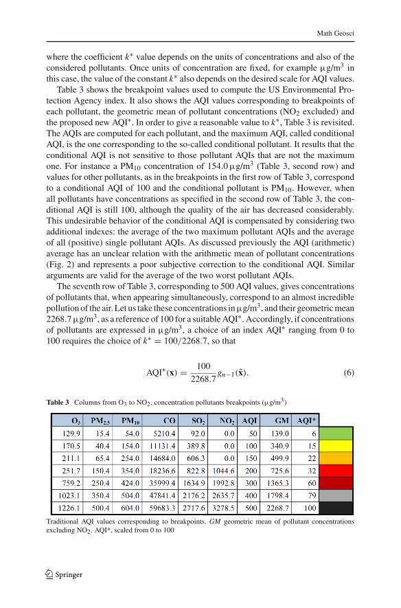
where the coefficient k∗ value depends on the units of concentrations and also of theconsidered pollutants. Once units of concentration are fixed, for example µg/m3 inthis case, the value of the constant k∗ also depends on the desired scale for AQI values.

Table 3 shows the breakpoint values used to compute the US Environmental Pro-tection Agency index. It also shows the AQI values corresponding to breakpoints ofeach pollutant, the geometric mean of pollutant concentrations (NO2 excluded) andthe proposed new AQI∗. In order to give a reasonable value to k∗, Table 3 is revisited.The AQIs are computed for each pollutant, and the maximum AQI, called conditionalAQI, is the one corresponding to the so-called conditional pollutant. It results that theconditional AQI is not sensitive to those pollutant AQIs that are not the maximumone. For instance a PM10 concentration of 154.0µg/m3 (Table 3, second row) andvalues for other pollutants, as in the breakpoints in the first row of Table 3, correspondto a conditional AQI of 100 and the conditional pollutant is PM10. However, whenall pollutants have concentrations as specified in the second row of Table 3, the con-ditional AQI is still 100, although the quality of the air has decreased considerably.This undesirable behavior of the conditional AQI is compensated by considering twoadditional indexes: the average of the two maximum pollutant AQIs and the averageof all (positive) single pollutant AQIs. As discussed previously the AQI (arithmetic)average has an unclear relation with the arithmetic mean of pollutant concentrations(Fig. 2) and represents a poor subjective correction to the conditional AQI. Similararguments are valid for the average of the two worst pollutant AQIs.

The seventh row of Table 3, corresponding to 500 AQI values, gives concentrationsof pollutants that, when appearing simultaneously, correspond to an almost incrediblepollution of the air. Let us take these concentrations inµg/m3, and their geometricmean2268.7µg/m3, as a reference of 100 for a suitableAQI∗. Accordingly, if concentrationsof pollutants are expressed in µg/m3, a choice of an index AQI∗ ranging from 0 to100 requires the choice of k∗ = 100/2268.7, so that

AQI∗(x) = 100

2268.7gn−1(x̂). (6)

Table 3 Columns from O3 to NO2, concentration pollutants breakpoints (µg/m3)

Traditional AQI values corresponding to breakpoints. GM geometric mean of pollutant concentrationsexcluding NO2. AQI*, scaled from 0 to 100

123

Math Geosci

Fig. 5 AQI∗ values vs AQI values at the traditional breakpoints (blue dots). Fitted line (red)

Fig. 6 AQI values (red) and AQI∗ values (blue) in time (months). Data set Madrid 2004–2013

Note that NO2 was not used for assessing the scale of AQI*, but the value2268.7µg/m3 including NO2 in the geometric mean is an almost incredible air pollu-tion situation.

Equation (5) is maintained as the definition of AQI∗ although the geometric meanincludes NO2. Figure 6 shows a comparison between AQI and AQI∗ values computedfor the reference data set (Madrid, 2004–2013); a secondary scale is used, as the corre-sponding scales are different although they are almost linearly related (Fig. 5). Figure6 also shows that air pollution in Madrid was in general very low (AQI roughly rangesfrom 10 to 30 and AQI* from 0.7 to 2.5). The AQI∗ ranging from 0 to approximately100 is proposed, so that the AQI∗ is easily interpreted. For instance, for the Madriddata set it is said that the AQI∗ values are in the interval (0.7,2.5) pollution over 100.

123

Math Geosci

4 Conclusions

Measures of air quality are based on concentrations of some given pollutants andconcentrations of suspended particles classified by size. Those concentrations arecompositional data and, consequently, they are properly analyzed using log-ratioapproaches. These analyses are based on log-contrasts, as they are scale invariant.

The log-contrast between concentration of non-pollutant components over pollu-tant components is taken as a proper dimensionless index of air pollution. A goodapproximation of this index is the logarithm of the geometric mean of concentrationsof air pollutants. The scale of this geometric mean is comparable to the traditionalAQI scale.

A first approach to a new air quality index ranging from 0 to 100 is proposed asAQI∗(x) = k∗gn−1(x̂), where k∗ is a constant depending on the units of pollutantconcentrations and gn−1(·) is the geometric mean of air pollutants concentrations.

Further modifications of the proposed index would require to determine weightingcoefficients of the proposed log-contrast according to health indicators.

Acknowledgments This work has been supported by the Ministerio de Economía y Competitividad ofSpain under projects ENE2012-36871-C02-01, partially funded by the European Union, and METRICSRef. MTM2012-33236; and within the framework of Consolidated Research Group of the Generalitat deCatalunya (Spain) AGAUR 2014-SGR-551. Authors also are thankful to Ayuntamiento de Madrid (Spain)for granting air pollution data.

References

Aitchison J (1986) The statistical analysis of compositional data. Monographs on statistics and appliedprobability. Chapman & Hall Ltd., London

Aitchison J, Egozcue JJ (2005) Compositional data analysis: where are we andwhere shouldwe be heading?Math Geol 37(7):829–850

Bishoi B, Prakash A, Jain V (2009) A comparative study of air quality index based on factor analysis andUS-EPA methods for an urban environment. Aerosol Air Qual Res 9:1–17

Bruno F, Cocchi D (2002) A unified strategy for building simple air quality indices. Environmetrics 13:243–261

Egozcue JJ (2009) Reply to “On the Harker variation diagrams;..” by J. A. Cortés. Math Geosci 41(7):829–834

Egozcue JJ, Jarauta-Bragulat E (2014) Differential models for evolutionary compositions. Math Geosci46(4):381–410

Egozcue JJ, Pawlowsky-Glahn V (2005) Groups of parts and their balances in compositional data analysis.Math Geol 37(7):795–828

Egozcue JJ, Pawlowsky-Glahn V (2011a) Análisis composicional de datos en ciencias geoambientales.Boletín Geológico y Minero 122(4):439–452

Egozcue JJ, Pawlowsky-GlahnV (2011b)Basic concepts and procedures. In: Pawlowsky-GlahnV,BucciantiA (eds) Compositional data analysis. Theory and applications. Wiley, New York

Pearson K (1897) Mathematical contributions to the theory of evolution on a form of spurious correlationwhich may arise when indices are used in the measurement of organs. In: Proceedings of the RoyalSociety of London LX, pp 489–502

Plaia A, Di Salvo F, Ruggieri M, Agró G (2013) Amultisite-multipollutant air quality index. Atmos Environ70:387–391

Plaia A, Ruggieri M (2011) Air quality indices: a review. Rev Environ Sci Biotechnol 10:165–179Russo A, Soares A (2014) Hybrid model for urban air pollution forecasting: a stochastic spatio-temporal

approach. Math Geosci 46:75–93

123

Math Geosci

The World Bank (2013) Report. on line. data.worldbank.org/indicator/SP.URB.TOTL.IN.ZSvan den Elshout S, Léger K, Nussio F (2008) Comparing urban air quality in europe in real time. A review of

existing air quality indices and the proposal of a common alternative. DCMR Environ Int 34:720–726

123