air quality atmospheric resources - york...
TRANSCRIPT
FINAL REPORT
Phase 1: Background Document
Air Quality &
Atmospheric Resources
Submitted to
The National Round Table on the Environment and the Economy
Environmental Sustainable Development Indicator Initiative
iv
BY
1 y
DSS Management Consultants Inc.
November 26,200l
DSS Management Consultants Inc. Designers of Decision Support Sysfems
November 26,200l
Ms. Carolyn Cahill Policy Advisor National Round Table on the Environment and the Economy 344 Slater St. Suite 200 Ottawa, ON KlR 7Y3
Dear Ms. Cahill:
Re: NRTEE’s Environment and Su$ainable Development Indicators (ESDI) Phase 1 Background Document - Atmospheric Services Indicators Our File No. 296-l Contract #: NRT-2001108
Following is the background report for the above project. This report documents the results of our background research findings as requested in the terms of reference. This report provides a reasonable basis for cluster group members to gain an understanding of the ciment state of development of atmospheric services sustainable development indicators.
Throughout the ‘report, considerable effort has taken to avoid reaching conclusions as to the merits of one SDI relative to others. This has not been easy. This being said we did not fïnd any SDI which is currently in use which appears in our view to satisfy a11 of the requirements that the NTREE has established for a national-level SDI for atmospheric services. Hopefully the SDIs which are included in this report Will be useful for the cluster group to arrive at their recommendations for a national-level atmospheric services SDI.
Yours truly, ,
C.C. Claire Applevich
1886 Bowler Drive, Pickering, ON LlV 3E4 Telephone: (905) 839-8814, Fax 839-0058
Table of Contents
Covering Letter .............................................................................................................................................. I
Table of Contents ......................................................................................................................................... II
List of Acronyms ......................................................................................................................................... III
I INTRODUCTION.. ............................................................................................................................... 1 1.1 BACKOROUND.. .................................................................................................................................. 1 1.2 PURPOSE ............................................................................................................................................ 1 1.3 SCOPE.. ............................................................................................................................................... 1 1.4 METHODOU)GY .................................................................................................................................. 2 1.5 REPORT ORGANIZATION.. ............................................................. ;. .................................................... 3
2 Ambient Air Quality and Human Health.. ........................................................................................... 3 2.1 SNGLE POLLUTANT INDICATORS.. ..................................................................................................... 3
2.1.1 Data Availability.. ..................................................................................................................... 4 2.1.2 Calculation Issues.. ................................................................................................................... 5
2.2 MD<ED POLLUTANT INDICATORS.. ...................................................................................................... 6 2.2.1 AcidRain .................................................................................................................................. 6 2.2.2 smog.. ....................................................................................................................... ......... .... 7 2.2.3 Greenhoue Gas Concentrations.. .......................... .............................................. .:. ....... ....... 8 2.2.4 Ozone-depleting Substances.. ................................................................................................... 9
2.3 AIR QUALITY INDEX ........................................................................................................................ 10 3 Emissions of Global Pollutants .......................................................................................................... II
3.1 GHG EMISSIONS.. ............................................................................................................................ 12 3.1.1 Basic GHGSDIs.. ................................................................................................................... 12 3.1.2 VariantsofGHGSDIs.. .......................................................................................................... 13
3.2 STRATOSPHERIC OZONE DEPLETION ................................................................................................ 14 4 Other Forms of SDIs .......................................................................................................................... 15
4.1 HUMAN HEALTH .............................................................................................................................. 15 4.2 CLIMATE CHANGE.. .......................................................................................................................... 16 4.3 MEASURES OF DIRECT EPFBCTS ....................................................................................................... 17 4.4 P”BLIC CONCBRNS.. ......................................................................... I ............................................... 18 4.5 RESOURCE CONSUMPTION PATTERNS .............................................................................................. 19 4.6 ECONOMIC DAMAGE MEASURES.. .................................................................................................... 20
5 Concluding Observations.. .................................................................................................................. 21 5.1 ABIJNDANCE OF AMBIENT AIRQUALITY INFORMATION .................................................................. 21 5.2 ABIJNDANCE OF POLLUTANT EMISSIONS INFORMATION .................................................................. 22 5.3 LMKAGES BETWEEN EMISSIONS AND AMEXENT AIR QUALITY ........................................................ 22 5.4 ABSENCE OF FORECASTING.. ............................................................................................................ 23 5.5 INDOOR AIRQUALITY GAP.. ............................................................................................................. 23 5.6 CONNECTIONS TO HUMAN HEALTH ................................................................................................. 24
References.. .................................................................................................................................................. 25 Appendir A.. ................................................................................................................................................. 31 AppmdoC B ................................................................................................................................................... 36
AB AQI AQW AR ARS ASL ASM BC BEN2 CAPMoN CASA CH4 CO CO2 DOE DRWED DFAE EC ENV EPA ESDI GDP GWP GHG GPI H2S HD HFCs HW IADN IQUA MB MC MWLP MRTSD NAPS ns NB NEIS NF NO2 NRTEE NS NT 03
iv
LIST OF ACRONYMS
Alberta Air Quality Index Air Quality Valuation Mode1 Acid Rain Arsenic Aerosol Asthma British Columbia Benzene Canadian Air and Precipitation Monitoring Network Clean Air Strategic Alliance Methane Carbon Monoxide Carbon Dioxide Department of the Environment Department of Resources, Wildlife and Economie Development Department of Fisheries, Aquaculture and Environment Environment Canada Environment Environmental Protection Agency Environment and Sustainable Development Indicators Grass Domestic Product Grass World Product Greenhouse Gases Genuine Progress Indicator Hydrogen Sulphide Hospital Discharges Hydrofluorocarbons Hamilton-Wentworth Integrated Acid Deposition Nehvork Index of the Quality of Air Manitoba Measuring Connnunity Success and Sustainability Ministry of Water, Land and Air Protection Manitoba Round Table on Sustainable Development National Air Pollution Surveillance not specified New Brunswick National Environmental Indicator Series Newfoundland and Labrador Nitrogen Dioxide National Round Table on the Environment and Economy Nova Scotia North West Territories Ozone
Y
iv Y
03D ODR OMOE ON PAH Pb PE PFCs PM10 PM2.5 PQ SDI SF6 SK SMG SO2 svoc THC TO TOMB TOX TRS TSP UK UV voc WA YK
Ozone Depleting Ambient Air Odour Ontario ,Ministry of the Environment Ontario Polycyclic Aromatic Compounds Lead
Prince Edward Island Perfluorocarbons Particulate Matter (particulates with diameters < 10 micrometres) Particulate Matter (particulates with diameters < 2.5 micrometres) Quebec Sustainable Development Indicator Sulphur Hexafluoride Saskatchewan Smog Sulphur Dioxide Semi Volatile Organic Compounds Total Hydrocarbons Toronto Toxic Organic Micropollutants Toxins Total Reduced Sulphur Total Suspended Particulate United Kingdom Ultra Violet Volatile Organic Compounds Washington State Yukon
1 INTRODUCTION
1.1 Background
This report has been prepared for the National Round Table on the Environment and Economy (NRTEE) as part of its Environment and Sustainable Development Indicators (ESDI) initiative.
This is one of a number of similar reports prepared for different sectors or clusters for which
Sustainable Development Indicators (SDI) are being evaluated/developed and recommended for
adoption. These other clusters include renewable and non-renewable natural resources, land and
soils, water resources and human capital.
7.2 Purpose
This report Will serve as a technical reference for the atmospheric services cluster group. No
attempt has been made to undertake any comprehensive comparative analysis of the SDI?
described in this report. Instead, key information concerning each indicator or indicator set is provided. This information is designed to assist the cluster group members in developing their
assessment of candidate indicators.
1.3 Scope
This inventory has focused on Canadian SDIs and related databases. SDIs developed by foreigo
organizations are included where appropriate but an exhaustive search of a11 SDIs developed by
jurisdictions and organizations outside of Canada has not been undertaken.
Three specific aspects of atmospheric services are the focus of this report, namely.
0 Ambient air quality and human health effects
t The tenn “sustainable development indicator (SDI)” is used extensively throughout this report. Strictly speaking within the context of the overall NTREE ESDI initiative, SDI refers to indicators satisfyiig the requirements of a sustainable development indicator within a natural capital framework. None of the indicators reviewed in tbis report satisfied these requirements. Accordingly, readers are advised to be aware that the term SDI is used less rigorously in tbis background report.
2
ii)
iii)
Air emissions having transboundary or global implications for ecosystem health
and human health Demand on the atmosphere for environmental services (i.e., primarily gaseous
waste assimilation/dispersion).
The latter two aspects are tied directly to pollutant emission rates whereas the fïrst is tied to
ambient pollutant concentrations. Clearly, a strong link exists between emissions and ambient
concentrations. These linkages among SDIs need to be considered by the cluster group members.
For the purposes of this report, however, these linkages are not evaluated. Instead each of the
three aspects of air resources is examined independently.
1.4 Methodology
The NRTEE provided much valuable information at the outset of this project. Some cluster
group members also provided suggestions as to additional information and data sources. Al1
sources relied on in preparing this report are listed in the references section. As well, Web site
addresses are provided in Appendix A for a11 SDI information collected through the Internet.
Most of research was done via the Internet. Some published sources not digitally available were
also examined but a comprehensive review of this literature has not been undertaken.
For the purposes of this background report, persona1 contact with representatives of most
organizations involved in developing air quality policy and SDIs has proven not to be necessary. Adequate information to characterize the curent state of knowledge and the availability of
support& data has generally been available through the Internet and other publicly available
sources. As the cluster group narrows its focus on candidate SQ&, direct contact with some
organizations and data managers Will likely be necessary. Contact information has been collected
for each organization with this potential need in mind.
A key part of this report is to provide an outline of the availability of the data required to
calculate SDI values. The NRTEE provided the latest version of databases for environmental
analysis (CCME, 1998) and the latest summary of the National Pollutant Release Inventoty
(Environment Canada, 1999). The former source is particularly comprehensive and easily
3
accessible. This database was a primary basis for determining the availability of key data to
estimate atmospheric services SDI values.
1.5 Report Organizafion
The following report has been organized into three main sections. The tïrst reviews the
availability of SDIs based on ambient air quality measures. The second examines the availability of SDIs based on pollutant emission levels. The third section discusses a range of SDIs that do
not fit into either of the preceding categories. Each section reviews systematically, those SDIs
currently being used or proposed for use and the supporting data available to calculate SDI
values.
The final section of the main body of the report sets out some concluding observations arising
from OU research on atmospheric services SDIs.
Appendix A provides more detailed information in summary chat? form for a number of
atmospheric services SDIs.
2 AMBIENT AIR QUALITY AND HUMAN HEALTH
This section reviews those SDIs which are based on, or directly connected to, measures of
ambient air quality. This review starts with the simplest SDIs, namely those based on absolute
measures of single pollutants. Several variants of these SDls are based on the degree or frequency of exceedance of pre-set air quality criteria or guidelines. The next level of SDIs
reviewed involves combinations of multiple pollutants (e.g., acid rain and smog). The final level
of complexity includes SDIs based on some form of index.
2.1 Sing/e Pollutant Indicators
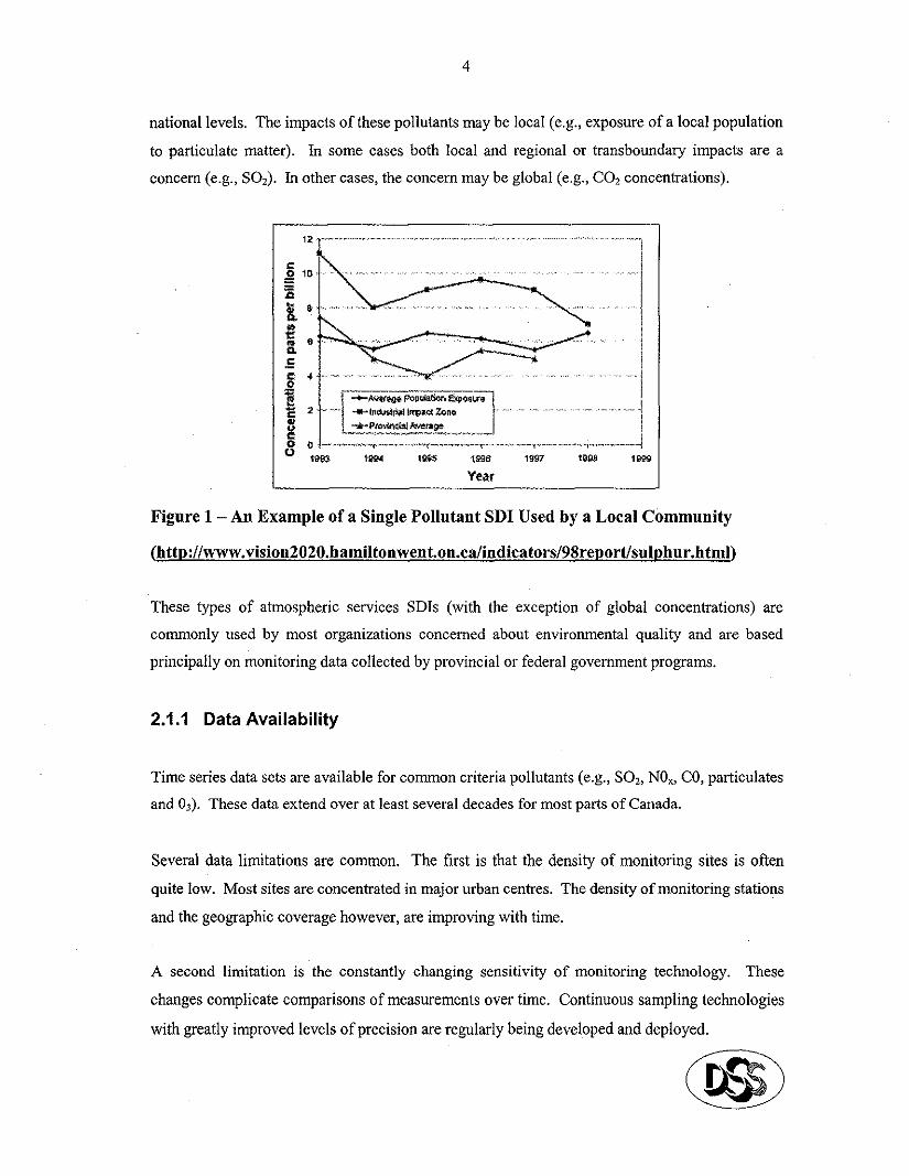
These indicators are the simple& in concept and calculation. Figure 1 is an example of the results
of such an indicator for a local community. Similar indicators are reported at the provincial and
4
national levels. The impacts of these pollutants may be local (e.g., exposure of a local population
to particulate matter). In some cases both local and regional or hansboundary impacts are a concem (cg., S02). In other cases, the concern may be global (e.g., CO2 concentrations).
Figure 1 -An Example of a Single Pollutant SDI Used by a Local Community
These types of atmospheric services SDIs (with the exception of global concentrations) are
commonly used by most organizations concerned about environmental quality and are based
principally on monitoring data collected by provincial or federal govemment programs.
2.1.1 Data Availability
Time series data sets are available for common criteria pollutants (e.g., SOz, NO,, CO, particulates and 0,). These data extend over at least several decades for most parts of Canada.
Several data limitations are common. The fïrst is that the density of monitoring sites is often
quite low. Most sites are concentrated in major urban centres. The density of monitoring stations
and the geographic coverage however, are improving with time.
A second limitation is the constantly changing sensitivity of monitoring technology. These
changes complicate comparisons of measurements over time. Continuous sampling technologies
with greatly improved levels of precision are regularly being developed and deployed.
5
A third complication is changes to the actual parameters being measured. For example, the focus
of particulate matter measurements moved from total suspended particulates to PMia. Now PM2.5
is considered to be the primary contributor to cardio-respiratory illnesses associated with air
pollution (and some more recent suggestions are being made that PM,.,, is the principal
constituent of concem). However historical PMî.S concentrations need to be interpolated from
measurements of PMia or total suspended particulates since this fraction of suspended particles
was not monitored extensively. This size fraction has begun to be measured extensively more
recently.
2.1.2 Calcuiation issues
As the scale of the area increases to which an ambient air quality SDI applies, data from multiple monitoring sites typically need to be incorporated in the calculation of the SDI value. This is
certainly the case when SDIs are being proposed having a national scope. The question arises as
to how best to weight or average disparate readings from multiple monitoring sites.
This issue is particularly acute in the case of global concentrations of individual greenhouse gases
(GHG). In this case, the most common solution is to use data from standard reference sites (e.g., Hawaii and northem Canada) that are far removed from the influence of signitïcant local’
emissions. Selecting such reference sites avoids the issue of averaging disparate readings from
multiple monitoring stations.
This option works for global pollutant concentrations but is not adequate where local variations
are signitïcant. Where human health impacts are a concem, weighting readings based on the size
of the exposed population has been proposed. In any event some form of averaging is required in
cases where large geographic amas are involved. None of the single pollutant SDIs examined
deals directly with this weighting issue, at least in a rigorous way in terms of expected human
health impacts.
Another calculation issue arises when dealing with temporal variations. Many SDIs are typically
reported on an annual basis, at least those used to track long-tetm trends. Considerable variation
from day to day and season to season is common with many pollutants.
6
This mises a similar issue with regards to weighting observations from different points in time.
One solution used with some SDIs is to track the number of hours or days a pre-set concentration is exceeded. These measures do trot yield concentration values but instead result in a tally of
occurrences. This approach fails to distinguish between marginal exceedances and large
exceedances but it does provide-a relatively simple means to calculate cumulative annual values
for these SDIs. Similarly, a simple average may obscure significant pollution incidents having
large potential for negative impacts.
None of the SDIs reviewed dealt fully with the issue of intra-ammal variations in pollutant
concentrations, at least with respect to variations in human health risks.
2.2 Mixed Pollutan t Indica tors
The four most common multiple pollutant SDIs are for acid rain*, smog, greenhouse gases and
ozone-depleting substances. Each of these categories of SDIs is examined individually.
2.2.1 Acid Rain
Two principle sources of acid rain are sulphur compounds (cg., sulphates) and nitrous oxides.
Both cause precipitation to be acidic and cari lead to damages to natural ecosystems and produced
capital (e.g., exposed surfaces of buildings and structures).
Some SDIs are based on measurements of wet deposition of one or both types of compounds.
These different pollutants cari be systematically combined based on the acidifying potential of each constituent chemical. These chemical relationships are well understood, although their net
effect on ecosystems may differ given differences in their chemical behaviour within the natural
environment.
Concern about acid rain began more than two decades ago, particularly in eastem Canada.
Extensive acid rain monitoring systems bave been in place since that time. As well, measurement
* The term “acid rain” is used hem although the tertn “acid deposition” is technically more accurate.
techniques and technologies have been well retïned and are now fairly standardized. As a result,
an extensive monitoring dataset is available to calculate historic acid rain SDI values and to
develop trend-over-tinte analyses.
One of the major concerns with acid rain has been its impact on freshwater aquatic ecosystems.
These impacts are a result of both short-term acid puises t’particularly during the spring freshette)
and due to long-term aciditïcation of watershed systems and the graduai decline in lake
neutralizing capacity. These phenomena are higbly site-specifïc. TO simplify the task of
determining the signitïcance of acid deposition rates, critical load values have been estimated. These critical load limits are the forecast maximum annual cumulative loading rate which cari be
sustained and Will still provide adequate protection for 95% of the lakes in sensitive watersheds.
Some acid rain SDIs are based on the number and/or magnitude of exceedances of these critical
loads. As is the case with other SDIs which measure exceedance of a pre-set standard or
criterion, the reliability of the SDI hinges largely on the adequacy of the standard. This is
particularly the case with acid rain. By defïnition, the critical load approach involves accepting
the expectation that 5% of the lakes in a watershed Will be aciditïed. Unless a standard is based
on an absolute threshold concentration or loading rate (i.e. a level below which no damage Will
occur, as opposed to no noticeable damage), some damages may occur even if the standard is not
exceeded. The extent to which this outcome is consistent with the concept of sustainable
development and conserving our natural capital for future generations is debatable.
A good example of this dilemma is the health effects associated with 0, and PM!,,. In both cases, national and provincial standards bave been set. On the other hand, current scientifïc evidence
suggests that an effect threshold does not exist. In other words, concentrations below the
established standard do cause human health impacts. In the case of acid rain, an “acceptable” damage rate is inferred by the standard. The standard does trot imply no damage if it is not
exceeded.
2.2.2 Smog
Smog is included in this section since this term is commonly used in the media. No technical definition or measurement of smog was found. Instead smog is a general term referring to the
8
combined effects of ground level ozone and particulate matter. These effects may be moderated
by the presence of other pollutants, as well as by temperature and humidity.
Some jurisdictions bave “smog” monitoring programs (cg., Ontario, British Columbia) and daily
air quality conditions are rated according to descriptive categories (e.g., good, fair, poor)
pertaining to the smog level. On the basis of the expected health risks of these pollutants, a
“smog alert” may be issued.
However, no quantitative measures of “smog” levels are reported. Likewise, a standard unit of
measure for smog per se was not found. Instead, where quantitative reporting of smog does exist,
the measures are typically based on ground level ozone or particulate matter concentrations.
The City of Toronto has based its smog SDI on the “annual number of bad smog days” (i.e., smog
alert days). This is similar to the approach used by some jurisdictions with air quality indices.
This type of smog SDI defers to the provincial government the task of synthesizing the various
weather parameters and associated forecasts for smog constituents to arrive at a smog rating. A
clear and consistent quantitative basis for making these determinations was not found.
2.2.3 Greenhouse Gas Concentrations
A number of gases (e.g., CO*, methane, nitrous oxides, some volatile organic compounds)
increase the insulative capacity of the atmosphere. As the insulative capacity increases, changes
in climate become increasingly probable (i.e., global warming). The combined effect of a11 GHG
determines the change in insulative capacity.
Some GHG and climate change SDIs involve reporting changes in ambient concentrations of each individual constituent gas. However, a common practice is to express each type of gas, in
CO2 equivalent units of measure. While the precise equivalency relationships are a source of
some uncertainty, using equivalency measures allows the combined insulative effect of a11 GHGs
to be estimated. This strategy has been used to track.and make aggregate comparisons of GHG
emissions but no SDI for ambient GHG concentrations was found which used this unit of measure.
9
Records of atmospheric CO* are available for over four decades. Data for other significant types
of GHG go back two decades or more. As a result, reliable trends-over-time bave been estimated.
Given the high level of public concern about climate change, continued and more intensive
monitoring of GHGs emissions and atmospheric concentrations cari be expected in the future. As
well, estimates of benchmark prehistoric COa concentrations are continually being improved using
sophisticated sampling and measurement techniques (e.g., measurements of the concentrations of
gases in air bubbles trapped in glaciers).
2.2.4 Ozone-depleting Substances
Various anthropogenic gases (in particular halocarbons) interact chemically with ozone leading
to significant reductions in the protective stratospheric ozone layer. The chemistry of this
phenomenon has been well understood for several decades. Furthermore, a global action plan to
reduce the impacts of ozone-depleting substances has been in place for more than a decade.
Various indicators are monitoring the effectiveness of these actions.
Ozone layer depletion is a global phenomenon, the rate of which is partially determined by the
concentration of ozone depleting gases in the stratosphere. The higher is their concentrations, the
greater is the potential for reduction in the thickness of the ozone layer.
The halocarbons most chemically reactive with ozone are chlorofluorocarbons (CFCs).
Environment Canada tracks ozone depletion potential based on lower atmospheric concentrations
of two forms of CFCs (i.e., CFC-11 and CFC-12).
Atmospheric concentrations data for CFCs have been compiled hem 1977 to the present. These
data are from monitoring stations throughout the northern and southem hemispheres; the reliability of these data is high.
The implications of several calculational steps need to be considered. The atmospheric
concentrations are expressed as global annual means. Means are estimated by calculating a
simple average of periodic readings from each station. This averaging process does obscure local and short-term variations but is not expected to alter significantly the interpolation of the overall trends over time with this SDI.
10
A second consideration is that Environment Canada reports separate SDI values for CFC-11 and
CFC-12. Since both bave-an ozone-depleting potential of 1.0, their combined impact is equal to
the sum of the two concentrations.
Finally, these measurements deal only with these two CFCs and not with global atmospheric
concentrations of other known ozone-depleting substances. Accordingly, the overall ozone-
depleting potential of the ambient concentration of a11 contributing halocarbons cannot be tracked
dire&’
2.3 Air Quality Index
The use of some form of air quality index3 (AQI) is common with most jurisdictions. The
advantage of an AQI is that air quality conditions involving multiple pollutants, varying
concentrations and differing degrees of impact cari be expressed through a single easily
understood value. TO further simplify matters, a normalized scaling system is often used. The
resulting values for the AQI are grouped then into broad descriptive categories (cg., good, fair,
poor).
A fairly standard procedure for calculating AQIs exists among federal and provincial
jurisdictions. Concentrations of common criteria pollutants are compared to established
guidelines or objectives. The difference between measured and threshold4 concentrations is
calculated and expressed as a relative’measure. The pollutant with the highest (i.e., worst)
relative measure is used as the basis on which to estimate the AQI for a given day or other time
period.
While the term “index” is used in this context, technically this is a misnomer. The AQI is not a composite value for multiple pollutants. Instead the AQI is a relative measure for only one pollutant, albeit, the one expected to produce the most negative impacts (Le., the pollutant exceeding the most above the established tiximum concentration). ’ The tlueshold concentrations set out in air quality standards and guidelines are closely linked to expected negative impacts on human health and the natual environment. Often these tbresholds are net in fact no- effecl fhresholds but are instead, maximum-acceptable-effects thresholds. This distinction is important from a sustainability perspective.
11
AQI is used primarily as a public communication device. AQI values are rarely used directly in
the development or analysis of air pollution policies. Instead, detailed analyses of the expected
impact of policy options are normally based on the individual constituent pollutants, their
expected changes in ambient concentration and the associated damages to human health, built
capital and the natural environment. Nonetheless conceptually at least, AQI values could be used
as a surrogate for potential damages and could serve as a useful SDI.
Several critical assumptions underlie this approach. Of particular note, the methodology ignores
any synergistic or cumulative effects of multiple pollutants. Moderately high concentrations of
several criteria pollutants may pose greater risk than having one pollutant with a moderately high
concentration and a11 the others at quite low relative levels. A conventional AQI would not reflect this difference in the risk of negative impacts.
Calculating AQIs leads to many of the same issues described for single pollutant SDIs (i.e.,
spatial and temporal averaging problems, particularly at a national level). As well, air quality
standards vary from jurisdiction to another making aggregation of AQI measures across
jurisdictions difficult. Likewise, to develop trends over time, adjustments would be needed to reflect air quality policy changes affecting the threshold values. Changing the threshold values
Will alter the AQI values.
Historical monitoring data for criteria pollutants are available for several decades although there
are limitations in these databases as discussed in Section 2.1 .l. Nonetheless, data availability is
nota limitation for using AQIs for atmospheric services SD&.
3 EMISSIONS OF GLOBAL POLLUTANTS
Emissions are another means to track the demands placed on local, national and global air resources by the economy. This section examines in particular, emissions of global pollutants.
Two categories of global pollutants are included, namely emissions of GHG and pollutants
causing stratospheric ozone depletion. Since the concem regarding these types of pollutants is
with ‘respect to changes in global atmospheric concentrations (i.e., total loading as opposed to
12
local ambient concentration impacts), some of the calculational issues discussed in the preceding
section do notarise. Emission loads from widely dispersed sources cari be simply added to track
changes in global loading rates.
The different forms of SDIs developed to track each of these two global air pollution issues are
discussed in the following subsections.
3.1 GHG Emissions
This section examines,the basic SDIs used to hack GHG emissions. As well, more sophisticated
variants are discussed.
3.1.1 Basic GHG SDls
The simplest SDI for GHG emissions involves monitoring total emissions of specifïc GHG
constituents. The most common mehic used to report GHG emissions is CO2 equivalents.
An important data issue arises in this respect. Carbon dioxide has net been up to this time, a
criteria pollutant for which regulatory limits or reporting requirements bave been established. As
well, many sources of carbon dioxide emissions are not ,monitored, requiring, instead, a inductive
procédure to estimate emissions. A common approach is to estimate the consumption of rati
materials (in particular fossil fuels) associated with a particular sector of the economy or location.
These procedures provide reasonably reliable gross estimates of carbon dioxide emissions.
Extensive time series of data regarding national and provincial consumption rates of different
types of fossil fuels are generally available. Carbon dioxide emission factors are applied to each
fossil fuel type to generate historical CO* total loading estimates.
Some jurisdictions and organisations include other GHG emissions to estimate a total GHG loading rate. Ideally, aggregate measures should be based on CO* equivalentsy In some cases,
’ COI equivalents bave been estimated for a11 common GHG. Their insulative potential is expressed relative to an equivalent amount of COr For example, metbane has a COrequivalent value of 21. Therefore a 1 gm emission of metbane to the atmosphere is equivalent to an emission of 21 gm of CO*.
13
however, the total combined mass of emissions is reported irrespective of variations in insulative capacity arnong individual constituent pollutants.
3.1.2 Variants of GHG SDls
Many variants of the basic total emissions loading GHG SDIs bave been developed. For
example, Statistics Canada is using a combined measure of GHG emissions and household
expenditures. The total annual emissions of carbon dioxide, methane and nitrous oxides expected
to be released by the production and consumption of a standard amount of household goods is
estimated and expressed in CO2 equivalents. By multiplying this GHG emission rate by total
annual household expenditures, a total load of GHG attributable to annual household
expenditures isestimated. This SDI is distinct from a11 others examined in that it ties directly
elements of GHG emissions with signitïcant elements of the economy (i.e., household
expenditures).
An extensive data set is available for each of the components of this SDI, allowing trends over
time to be estimated.
Another variant has been developed by Environment Canada, referred to as a “carbon dioxide
intensity” SDI. This indicator reports carbon dioxide emissions relative to fossil fuel
consumptive rates. Changes in this SDI do not reflect directly changes in total GHG loading
rates. Instead, this SDI reflects the proportions of different fossil fuels consumed by an economy
and the carbon intensity of this fuel mix. For example, the higber the consumption rate of natural gas relative to other fossil fuels, the lower Will be the value for this indicator. This SDI is
insensitive to increases or decreases in the overall fossil fuel consumption rate of an econotny.
Extensive datasets are available to calculate the annuai values for this SDI.
The Alberta Genuine Progress Indicator (GPI) study reported GHG emissions trends by economic sector. A central tbmst of the GPI approach is to express the implications of pollution in physical
and economic terms. This study relied heavily on secondary sources to develop estimates of the
economic damage likely to be experienced as a result of total GHG emission loads. No direct
connection is made between expected levels of GHG and expected damages as is the case with
14
damage function models (see discussion in Section 4.6). Temporal trends were estimated in
terms of the annual economic damages of GHG (e.g., due to climate change). While these
estimates are quite approximate, they do offer the potential for direct comparison with the other
economic measures of wealth and well being commonly included in conventional economic
capital accounts.
3.2 Stratospheric Ozone Depletion
Various antbropogenic gases (primarily halocarbons) interact chemically with ozone leading to signifïcant reductions in the protective stratospheric ozone layer. The chemistry of this phenomenon has been well understood for several decades. Furthettnore, global action to reduce
the impacts of ozone-depleting substances has been in place for more than a decade. Various SDIs bave been used to monitor the effectiveness of these actions.
Halocarbons are highly stable and long-lived, some of the reasons why these gases were preferred
for various purposes (e.g., refrigeration). During use, the gases are not typically deshoyed. Instead, at the end of the productive life of the equipment in which they were used, these gases
were commonly released intact to the atmosphere.6 For this reason, a strong correlation existed
between the annual production of these gases and the ultimate emissions to the atmosphere. The
primary unknown related to when their release was likely to occur.
For these reasons, the total annual production of halocarbons has been selected by Environment
Canada as one SDI to track ozone-layer-depletion potential. Annual Gross Domestic Product
(GDP) is commonly used as a benchmark to interpret trends in total annual production. Including
GDP trends provides a means to track trends in production relative to overall economic output.
Environment Canada also produces estimates of the global production of ozone-depleting
substances and gross world product. Trends in worldwide production rates provide a measure of
the relative performance of the Canadian economy.
6 In Canada, environmental regulations are now in place prohibiting the intentiona release of CFCs fiom refridgeration units and similar types of machinery.
15
An extensive database for all of Canada is available since 1979 to back this SDI. These gases are
produced by a limited number of large manufacturers with good records of total production.
Trends over time in total annual CFC production bave been prepared by Environment Canada.
The major data-related issue involves the differing chemical reactivity among the different types
of halocarbons. As with GHGs, a common metric (Le., ozone-depleting potential) has been
developed for each gas. This ozone-depleting potential of each gas is reasonably well understood
and is not a large cause of uncertainty. Accordingly, aggregate measures of ozone-depleting
potential,for a diverse mix of halocarbons cari be reliably estimated.
4 QTHER FORMS OF SDls
This section discusses a number of SDIs relating to atmospheric services that are not based on
ambient concentrations or emissions of key pollutants. Theses SDIs have been grouped
according to the nature of the element being measured.
4:l Human Health
A primary concern associated with air quality is impacts on human health. A number of SDIs have been employed to track health impacts associated with air quality.
For example, the Region of Hamilton-Wentworth is tracking annual per capita hospitalization
rates as an indicator of air quality. Poor air quality is expected on average to increase
hospitalization rates and vice versa. Data for this SDI are readily available from provincial health
tare and population databases. Correlating trends in this SDI directly to changes in air quality is diftïcult, particularly when multiple pollutants may a11 be contributing differently to
hospitalization rates.
A similar type of SDI proposed for local community use is annual sales of medicines used to treat
illnesses commonly associated with poor air quality (e.g., asthma/allergy treatment). The inferred
relationship with air quality is similar to that underlying the hospitalization rate SDI. In other words, medicine sales are expected to climb when air quality declines and vice versa. An
16
advantage of this SDI is that at least theoretically, trends over time Will reflect the acute impacts
of air quality on asthma/allergy attacks. As well, chronic exposure to air pollutants (which may
lead to an increase in the prevalence of asthma in an exposed population) Will also be reflected by
long-temr trends in medicine sales. More specifically, the overall frequency (i.e., health risk) of
asthma attacks per poor air quality incident Will be expected to increase as chronic exposure
increases the prevalence of these diseases in a population.
Comprehensive data for medicine sales are not maintained in a central repository, particularly for
over-the-counter, non-prescription drugs. Accordingly, the proponents of this SDI indicate that
independent data needs to be collected at the community level. No national-level estimates for
this type of SDI were found.
Interpretation of trends in this type of SDI could be difficult due the high potential for
confounding factors. Likewise due to the diffculty in obtaining data, historical trends cannot be
estimated.
Life expectancy at birth has been proposed as an SDI in Alberta. Air pollution does increase the
risk of death in some segments of a population and Will, therefore, affect life expectancy. The
difficulty is the multiplicity of confounding factors, which may increase (e.g., improved health
tare and medical techniques) and decrease (e.g., increased substance abuse) life expectancy.
Life expectancy data are widely available and regularly used, particularly by the insurance
industry. A major diftïcuhy with these data is that life expectancy values for a cohort cari only be
accurately calculated after a11 members of the cohort bave died. Accordingly, a lag between the
effect of air pollution on risk of death and life expectancy of a cohort Will delay policy actions if
this SDI is used as a primary measure of sustainability.
4.2 Climafe Change
Many indirect measures for climate change bave been proposed. The most direct climate change
SDI is trends in mean annual temperature. Data to calculate this SDI are available for an
extended timeframe given the universality of this weather measurement. The primaty
17
complications are 1) distinguishing long-term trends due to climate change from natural short-
term variations and 2) connecting long-term trends to the underlying causal factor(s).
Nonetheless, annual average temperature is a potentially powerful (if not the most powerful) SDI for climate change. This is partially due to the familiarity of the public with temperature
measurements and the direct connection to the concept of climate change.
A great divers@ of other types of climate change SDIs has been proposed. These range from the
average dates for such events as bird migrations to the frequency of catastrophic weather events
to the annual abundance of certain insect species. With a11 of these SDIs, the underlying
inference is that the timing and behaviour of many natural events are tied closely to overall
climate. Subtle trends in climate are expected to be magnified by the behaviour of these sensitive
natural events. These SDIs have been proposed for Britain and are not being used widely in
North America. However, the overall concept underlying these SDIs is transferable from one
geographic area to the next.
4.3 Measurek of Direct Effects
The concem with ozone-depleting substances is the potential for reduction in the effective
thickness of the stratospheric ozone layer. Environment Canada has tracked changes in the ozone
layer for an extended period of time. Long-term reductions in the thickness of the ozone layer are
considered symptomatic of unsustainable human activities. Reliable data to track trends in ozone
layer thickness are available from 1957. While some adjustments to some of the older data have
been necessary, a reasonable picture of long-term trends has been prepared.
As with many SDIs in this section, a major limitation in interpreting this SDI is tying observed
trends to the,underlying causal factors. For example without having accompanying information
on trends in ambient concentrations of ozone-depleting substances, one could only conclude
whether a long-term trend existed. This conclusion, however, would be insuffcient to decide on
the type and extent of policy initiatives needed to counter these trends. Likewise, anticipating the
impact on ozone layer thickness of expected increases in economic activity would be diffcult in
the absence of some connection to the underlying causal factors. From a policy development and analysis perspective, forecasts of the future thickness of the ozone layer need to be tied directly to
18
expected economic and related human developments. In this respect, using the thickness of the
ozone layer for an SDI is comparable to using temperature trends as an SDI for climate change.
Both need to be directly tied to the underlying causal factors.
A related SDI to ozone layer thickness is the UV index. This index is an indicator of the amount
of harmful UV radiation expected over the course of a day. ~The UV index generally increases as
the level of protection from the stratospheric ozone layer is reduced. Increases in UV radiation
exposure are closely connected to increased health risks.
The W index, however, is not a reflection only of ozone layer thickness but is also influenced by
precipitation, cloud caver, time of year and latitude. Accordingly, the W index varies
signitïcantly from place to place on a given day.
The UV index was developed in 1992 and has since been regularly forecast and measured
throughout Canada. As a result, trends over time are restricted to this period.
This SDI presents several calculational challenges. The flrst involves the difficulty of estimating
a meaningful representative national-level value. No method to aggregate local UV index values
across geographical areas has been developed. The possibility exists to use the type of shategies
discussed with air quality indices and individual pollutant SDIs (e.g., cumulative number of
exceedances of a specified level for discrete geographically uses) but this has not been proposed
at this time.
Despite these challenges, a UV index SDI could partially capture the combined effects of ozone
depletion and climate change (i.e., since weather conditions are a determining factor in the index
value).
4.4 Public Concerns
Several local community SDIs relating to air quality involve the level of concem expressed by
local residents. One SDI tracks odour complaints. Another tracks any complaints involving air quality.
19
A major obstacle with these SDIs is the absence of a central database containing records of public
complaints about air quality. Instead, estimating these SDIs requires targeted data collection
efforts. Accordingly, historical values for these SDIs are generally net available and trends over
time cannot be easily produced.
Another concem involves the potential insensitivity of these SDIs to the more subtle impacts of
air quality. Typically, quite sophisticated and extensive epidemiological studies are required to
detect and quantify human health impacts of air quality. Many of these impacts are not noticeable to highly trained medical practitioners, let alone casual observers.
4.5 Resource Consumption Patterns
Several atmospheric services SDIs have been proposed relating to resource consumption/use pattems, particularly relating to vehicular travel. Measures such as fuel consumption per capita
and vehicle miles per capita have been used to track consumption patterns and to infer indirectly
emission’rates of air pollutants. These SDIs provide a direct connection to the consumption
pattems of the individual and thus, cari be powerful tools for instigating behavioural changes.
Data on fuel consumption are readily available for an extended period. Trends in average per capita consumption rates cari be estimated fairly easily. In the case of annual average vehicle use,
the required data are much more diffcult to obtain. Accordingly, deriving historical SDI values
cari be problematic.
Similar types of SDIs have been proposed for monitoring GHG cycles and climate change
potential. For example, changes in cleared forest area, forest structure and even silviculture practices have been proposed to track changes in carbon sequestered in forest ecosystems.
Comprehensive data for these types of SDIs are generally net available in a suitable form from a
central (i.e., national or provincial) database. Forest caver and local management practices data
are available at the local forest unit scale. Obtaining these data to generate national values for
such SDIs would require an extensive data collection effort targeting individual forest management operations. Some of these data could ~also be derived from remote sensing
20
information. Nonetheless, this type of SDI relates more closely to the mandate of the renewable
resources cluster group.
4.6 Economie Damage Measures
This last group of SDIs has not been promoted tbrough sustainable development initiatives.
Instead, these SDIs bave been used in the past, primarily for policy analysis. More recently, some of these potential SDIs are being used more extensively also for public communication purposes.
Environment Canada and Health Canada bave sponsored for more than six years the development
of the Air Quality Valuation Mode1 (AQVM). The AQVM is a damage function mode1 designed
to forecast physical and economic damages associated with air pollution. Similar models, at least
in concept, were developed for acid rain in the 19.80s. As well, more detailed, community-
specific models bave been developed for use by local opinion shapers and decision makers (Le.,
Illness Costs of Air Pollution model). These types of models yield aggregated damage estimates
associated with air pollution expressed in physical and economic terms.
There are some similarities between these types of models and the basic valuation procedures used with the GPI approach. By including economic measures as well as physical measures of
damages, aggregation of expected impacts is facilitated. The tore of these types of models
consists of exposure/response functions7 derived from epidemiological studies. These damage
function models~are used to forecast quite specifïc types of impacts (e.g., premature mortality,
hospitalizations, damages to renewable resources) according to the nature and scope of the
exposure/response functions on which they are based.
These types of models are typically data intensive, at least in the developmental stages. Once
developed, their application is quite straightforward. A particularly valuable application for
sustainability reporting is estimating historical damage trends over time. The primary historical
data required for this application are ambient air quality conditions and the size and nature of fhe
’ An exposure/response fimction is a quantitative expression of the causal connections between exposure to air pollution and the resulting impacts. For example, a simple exposureiresponse function would be the expected increase in hospital admissions due to astbma attacks when ground-level ozone concentrations increase by 1 ppb. Exposure/response functions bave been developed for a wide range of air quality impacts on human health, built capital and valuable features of the natural environment.
21
exposed receptor population. Suitable historical data are available to produce such damage
estimates although considerable work may be required in some instances to compile suffciently
comprehensive datasets. TO date, these damage fonction models bave not been used extensively
for backcasting (the most common application of other SDIs). Instead, these models are used
primarily for forecasting exnected future damages expected with alternative air quality policies.
While some controversy continues to exist regarding the economic coefficients used in these
models (particularly for sensitive issues like risk of preniature mortality), improvements to these
economic coefficients are constantly being achieved. As ~11, much broader acceptance of the
value of producing economic measures of air pollution damages is evident. An advantage of
using these damage estimates as an SDI for atmospheric services is that they provide a ready
means to aggregate diverse types of air quality impacts using a rigorous and sound theoretical
framework. Doing SO permits the implications of policy alternatives and different economic
development paths to be clearly express-ad in famihar economic measures. These measures are
directly comparable to the measures used by policy analysts when considering economic and
social development alternatives.
5 CONCLUDING OBSERVATIONS
This section presents some observations arising from this review of existing atmospheric services
SDIs.
5.1 Abundance of Ambient Air Qoality Information
An extensive ambient air quality monitoring system has been in place in Canada for decades.
The network of sampling stations is being continually improved over time, both in ternis of the
density of sampling stations and the scope, frequency and precision of air quality measurements. The resulting databases provide adequate information to track hends over time for conventional
pollutants.
22
For these reasons, the availability of data is not a primaty barrier to developing ambient air
quality SDIs. Concentrations of individual pollutants and mixes of pollutants are being regularly
tracked at the national, provincial and local levels.
5.2 Abundance of PoIlutant Emissions Information
Environmental agencies regularly report historical, current and expected future pollutant
emissions when discussing air quality policy options. Likewise, an extensive regulatoty system is
in place, which requires major point sources of air pollutants to report emissions on a regular basis. These reports are maintained in central databases that are suitable for developing current
and historical estimates for emissions-based SDIs. The scope of pollutants and the reporting
requirements are being continually improved over time.
For these reasons, the availability of pollutant emissions data is not a barrier to developing
emissions-based SDIs. Emissions-based SDIs for individual pollutants have been estimated and
are being regularly tracked at the national, provincial and local levels.
5.3 Linkages Between Emissions and Ambient Air Quality
A primary limitation in developing SDIs useful for policy analysis is the diffculty in linking
expected emissions to changes in ambient air quality. Doing SO involves the application of
pollutant dispersiomatmospheric behaviour models which are data intensive, complex and are
sensitive to many stochastic variables (cg., wind pattems, temperature, precipitation). As well,
the geographic location of pollutant emissions sources has a large impact on air quality forecasts.
From a policy analysis perspective, managing ambient air quality is achieved by regulating pollutant emissions. For this reason, much focus is commonly placed on expected trends in
emissions. However, in terms of expected damages, ambient air quality is the determining factor.
In other words, direct links behveen emissions and ambient air quality are essential for SDIs to be
meaningful. Limitations in the ability to link emissions and ambient air quality translate into
significant limitations in developing atmospheric services SDIs useful for policy analysis.
23
Significant weaknesses in these linkages are evident with many of the atmospheric services SDIs examined.
5.4 Absence of Forecasting
A primaty requirement for policy analysis is the ability to estimate the expected future value of an SDI given alternate policy options. For example, when a new ntitional budget is announced,
expected impacts on key economic perfotmance indicators (cg., employment rate, interest rates,
GDP) are presented. In a similar fashion, expected impacts on atmospheric services SDIs need to
be tied directly to these types of broad-level policy decisions. Inherent to these forecasts is a
direct connection between key economic and social factors and the underlying causal factors
driving an SDI.
Quantitative projections of the expected future state of atmospheric services SDIs were trot
reported by any of the sources examined. Instead, only historical and current values were
typically reported. In some cases, expected trends were discussed but these narrative discussions
were not reflected in quantitative projections of the expected future state of individual SDIs.
The underlying causes for this pattem may be many. Nonetheless to date, the emphasis with
SDIs has been on tracking historical air quality and emissions trends over time and trot on
projecting expected future trends. TO switch focus Will require some adjustment in many SDI
repotting initiatives and some SDIs may be of limited value for such applications.
5.5 Indoor Air quality Gap
The great majority of atmospheric services SDIs deal with outdoor air quality. Indoor air quality
1) is often poorly correlated with outdoor air quality, 2) is often of much poorer quality than
outdoor air quality and 3) on average accounts for the major@ of the total exposure of individu& to air pollutants. Further complicating matters is the large variations in indoor air quality from one building to the next and the dearth of indoor air quality data for individual
buildings. Where such data do exist, they are not maintained in’central databases. These barriers
create a major challenge in developing comprehensive atmospheric services SDIs.
24
This report does not deal with indoor air quality SDIs. Few were encountered during the
background research. The sustainability issues relating to indoor air quality are much more
challenging than those relating to outdoor air quality, at least front a monitoring and reporting
perspective. The indoor air quality “gap” has been an issue for regulators for decades. Little
progress in filling this gap is evident in the SDI field at the present time.
5.6 Connections to Human Health
A primaty concem relating to air quality is the potential for negative human health impacts. Air
qua& guidelines, objectives and standards are often largely based on expected human health
impacts. Connections between most atmospheric services SDIs and human health, however, are
obscure and indirect. For example, trends over time in ground-level ozone concentrations are
commonly reported. While the relationship behveen ozone concentrations and respiratory illness
symptoms are discussed in general terms, SDIs based on annual average concentrations are
diffcult to translate into actual impacts.
A related factor in this respect is the role that exposure rate plays in expected negative impacts.
Human health impacts are connected directly to the number of people exposed and the frequency
of key risk factors in the exposed population (cg., age, illness history, activity pattem). These
types of factors are not reflected by typical atmospheric services SDIs. In other words, ambient
air quality or pollutant emission SDIs do not provide clear insight into expected human health
impacts.
This concem is exacerbated when simple avcrages arc used to aggregate pollutant measures
which vaty over space and time. Not surprisingly, human exposure potential varies significantly
from one sampling site and time to another. The more direct is the connections among pollutant
concentrations, human exposure and expected health impacts, the greater value an SDI Will bave
for policy analysis and~for providing a clear and unambiguous picture of sustainability trends.
25
REFERENCES
1.
2.
3.
4.
5.
6.
1.
8.
9.
Alberta Environment. 2001, Mobile Air Monitoring Lab (MAML) (1997-200 1). htta://~3.~ov.ab.calenv/airlmaml/~~ame.hhl
Alberta Round Table on the Environment and Economy. 1994. Creating Albert& Sustainable Development Indicators. httn://www.sustainablemeasures.com/Database/Albrt.html
Alberta Treasury, Performance Measurement. 2001. Sustainable Measures Indicator Project. Measup Annual Reports. (1998-2001): httn://www.treas.~ov.ab.ca/connnperfmeas/index.html
ANPA and WENCO. 2001, INDEX: 3rd International Congress on Environmental Indices and Indicators. Rome, Italy. Organized by Italian Environmental Protection Agency (ANPA) and Center for International Environmental Cooperation of Russian Academy of Sciences (lNENC0) httn://www.inenco.org/index conferences.html
British Columbia Ministry of Environment Lands and Parks. 1995. Emissions Inventory of Common Air Contaminants and Greenhouse Cases. h~:l/www.elp.~ov.bc.c~ep~endn~ar/airq~Ii~/invento~/subindex.h~l
British Columbia Ministry of Environment, Lands and Parka 1996. Air Monitoring Guidelines: Volume 1 Particulate Non-continuous. htto://www.elo.~ov.bc.ca/ep~epd~a/ar/pa~iculates/am~lnnc.h~l
British Columbia, Ministry of Water, Land and Air Protection. 2000. Environmental Trends in British Columbia: Air Quality Impacts (1994-1998), Greenhouse Gases (1970-2000). http://www.elp.gov.bc.ca/epd/enda/ar/vehicle/aqrfbc.html httn://www.elp.gov.bc.ca/spnl/soet7lt/etdf
CIBSIN Thematic Guides. 2001. Ozone Depletion and Global Environmental Change httn://www.ciesin.org/TG/OZ/oz-home.html
City of Hamilton 2001. Vision 2020. Sustainability Indicators: 1998 Background Report- Improving Air Quality (1993-1998). httn://www.vision202O.hamilton- went.on.ca/indicators/98reuort/ozone.html
10. City of Toronto Public Health. 2001. Toronto’s Public Health Status: A Profile of Public Health in 2001. Section 3. Air quality, P. 28. htto://www.citv.toronto.on.ca/health/ths 2001hesdf
11. Clean Air Strategic Alliance (CASA). 2001. Alberta Ambient Air Data Management System (AADMS) (1994-2001). http://www.casadata.org/AboutAAAi.htm
12. Ecological Indicators website. 2001. Ecological Indicators - Integrating Monitoring, Assessment and Management. (D. Eric Hyatt, Editor-in-Chief). httn://www.ecologicalindicators.orpi
26
13. Environment Canada and the Department of Fisheries, Aquacultnre and Environment of Prince Edward Island. 2001. Regional Smog Forecast for PEI. . httn://www.atl.ec.gc.caAveather/smog wa.html
14. Environment Canada, Air Quality Processes Research Division, The Meteorological Service of Canada. 2001. Integrated Atmospheric Deposition Network (IADN). hnp://www.msc.ec.ac.ca/arqn/iadn ecfm
15. Environment Canada, Analvsis and Air Oualitv Division Environmental Technology Center. 2001. National Air Pollution surveillance (NAPS) Network Canada’s National Smog (Gw Management Progmm (1974-2001). htm://www.etcentre.ora/naps/English/naps.html
16. Environment Canada, Atlantic Region. 1999. Trends in Acid Deposition in the Atlantic Region (1980-1999). Prepared by B. L. Beattie and C. Ro, Meteorological Service of Canada, Dartmouth, Nova Scotia. httn://www.atl.ec.ac.ca/Dollution/air.html
17. Environment Canada, Pollution Data Branch. 1997. Canada’s Greenhouse Gas Inventory: Emissions and Removals with Trends. Prepared by F. Neitzert. ISBN-0-662-27783-X httn://www.ec.gc.ca/pdb/gha/ehe docs/ah enandf
18. Environment Canada. 1998 National Environmental Indicator Series: Climate change. SOE Technical Supplement 98-3. httn://www.ec.nc.ca/ind/Enrrlish/Climateffech Suu/ccsu~Ol e.cfm
19. Environment Canada. 1999. Air Pollution: Acid Rain, Greenhouse Gases, Smog, Stratospheric Ozone and W Radiation.. http:/lwww.atl.ec.gc.ca/pollution/air,html
20. Environment Canada. 1999. National Environmental Indicator Series: Acid Rain. SOE Technical bulletin 99-3. httn://www.ec.rc.ca/ind/En~lisb/AcidRaitiulletin/arind1 e.cfm
21. Environment Canada. 1999. National Environmental Indicator Series: Stratospheric Ozone Depletion. SOE Technical Supplement 99-2. httn://www.ec.ec.ca/ind!Enalish/Ozone/Tech Sun/stsunl ecfm
22. Environment Canada. 1999. National Environmental Indicator Series: Urban Air Quality. SOE Technical Supplement 99-l. httn://www.ec.gc.ca/ind/English/Urb Air/Tech Sup/uasupl e.cfin
23. Environment Canada. 2001. “Enviroozine”: Environment Canada’s online newsmagazine. http://www.ec.~c.ca/envirozine/english/hme e.cfm
24. Environment Canada. 2001. Atlantic Smog Forecast. httn://www.ns.ec.sc.ca/weather/ozone.html
25. Environment Canada. 200 1. Pacifie ,200 1. httn://www.msc.ec.~c.ca/pacifïc2OOl/description e.html
26. Environment Canada. 200 1, UV Index. http://www.msc- smc.ec.gc.ca/uvindex/about uvindex e.html?CFID=2297502&CFTOKEN=60381462
27
27. Environment Canada. Air Quality Processes Research Division. 2001. Centres for Atmospheric Research Experiments (CARE). httn://www.msc.ec.ac.calaran/care e.cfm
28. Environment Quebec. 1999. Air Qua& in Québec (1975-1994): A Status Report. http://www.menv.gouv.qc.ca/air/qualite-en/index.htm
29. Environmental Treaties and Resource Indicators (ENTRI). 2001. Stratospheric Ozone Depletion: Treaties, Environmental Indicators, and National Responses. httn://sedac.ciesïn.or~/entri/guides/sec3-ozone.
30. Government of Alberta. 2001.2000/2001 Annual Report Alberta. Air Quality: Goal 16 - “Air Quality Days”. httn://www.cleanair.wehnet/whatsnew/index.html
31. GPI Atlantic (Genuine Progress Index for Atlantic Csnada). 1999. Introduction ta the GPI Gas Account. httn://www.gpiatlantic.org/sab15.shtml
32. GPI Atlantic. 1998. Measuring Sustainable Deveiopment: The Nova Scotia Genuine Progress Index: Framework, Indicators and Methodologies. hïro://~.~iatlantic.or~/pdf/contents/~ameworkcontents.udf
33. GPI Atiantic. 2001 .The Nova Scotia Greenhouse Gas Accounts for the Genuine Progress Index. httn://www.~iatlantic.ors/ab ghg.shtml
34. International Institute for Sustainable Development. @SD) 2000. Measurement and Indicators for SD. p
35. Manitoba Conservation, Manitoba Sustainable Development. 2000. Proposed Air Quality Indicators. ht~://www.susdev.eov.mb.ca/indicators/environmen~l/air.h~l
36. Manitoba Round Table for Sustainable Development. (MRTSD). 2001. Recommendations ta the Manitoba Govemment Regarding Provincial Sustainability Indicators. httu://www.susdev.gov.mb.ca/Reu-Sust-Ind.doc
37. Meteorological Service of Canada, Environment Canada. 2001. Canadian Air and Precipitation Monitoring (CAPMoN). httn://www.atl.ec.rrc.ca/msc/em/land oualitv.hhl#caumon
38. New Brunswick Deparhnent of the Environment and Local Govemment. 2000. An Introduction to Air quality in New Brunswick. httn://www.~b.ca/ela- eg1/0355/0007/AOE.ndf
39. New Brunswick Department of the Environment snd Local Government. 2000.The Index of the Quality of the Air (IQUA)(1979-2000) httn://www.gnb.ca/scriuts2/environm/air/GetValues.idc
40. Newfoundland and Labrador Environment. 2001. Mercury Depositional Program. httu://www.gov.nf.ca/env/env/pollprev/mercurv nropram deut env.asp.
28
41. Newfoundland and Labrador Environment, Environmental Science, and Monitoring Section. 2001. Acid Rain Program (1994-1998). httD://www.aov.nf.ca/env/env/nollprev/acid rain nroaram dent of el.aw
42. Newfoundland and Labrador Environment. 2001. Ozone Layer Protection Program. httn://www.aov.nf.ca/env/env/PollPrev/Ozone dept env.asp.
43. North Central Regional Center for Rural Development, Iowa State University. 2001. Aspen Institute’s Rural Economie Policy Program Measuring Community Success and Sustainability: An Interactive Workbook - (mdicator 1 Air Quality). http://www.aa.iastate.edu/centers/rdev/Communitv Success/indicator4-1 .html
44. Northwest Territories Resources, Wildlife. And Economie Development. 1998. Greenhouse Gas Emissions Forecast for the Northwest Territories. Prepared by Ferguson Simcoe Clark, Environmental Protection Service. httn://www.gov.nt.ca/RWED/librarv/eps/reuort~efr.ndf
45. Northwest Territories, Department of Resources, Wildlife and Economie Development (DRWED). 2000. Northwest Territories Air Quality Report (1999-2000). httn://www.aov.nt.ca/RWED/eps/udfs/99-OONWT Air Oualitvndf
46. Northwest Territories, Department of Resources, Wildlife and Economie Development. 1998. Carbon Dioxide Emission Reduction Measures (1990 to 1998). http://www.gov.nt.caiRWED/library/eps/cO2repo.pdf
47. Nova Scotia Department of the Environment. 1998. The Nova Scotia State of the Environment-Air Quality (1978-1998). htm://www.eov.ns.ca/envi/Soer/envdoc.pdf
48. Nova Scotia Environment and Labour. 2000. Air Quality Index for Halifax-Dartmouth. httn://www.aov.ns.ca/enla/rmep/erm.htm
49. Ontario Clean Air Alliance (OCAA). 2001. A Comparison of U.S. and Ontario Nitrogen Oxides Emissions. httn://www.cleanair.web.net/whatsnew/index.html httn://www.cleanair.web.net/whatsnew/archives.html
50. Ontario Ministry of the Environment. .2001. Air Quality and Climate Change: Moving Forward. htto://www.ene.pov.on.ca/envision/airclimate/airclimate.htm
5 1. Ontario Ministry of the Environment. 1997. Ontario Government’s Response to the United States Environmental Protection Agency’s (USEPA) proposa1 on changes to the national ambient air quality standards for particulate matter and ozone. httn://www.ene.aov.on.ca/envision/smog/index.htm
52. Ontario Ministry of the Environment. 1997. Proposa1 for an Interim Ambient Air Quality Criterion for Inhalable Particul&e Matter. httn://www.ene.aov.on.ca/proarams/nrounm.htm
53. Ontario Ministry of the Environment. 1998. Air Quality in Ontario: A Concise Report on the State of the Air Quality in Ontario (1980-1998). httn://www.ene.gov.on.ca/envision/techdocs/4054e.pdf
29
54. Ontario Ministry of the Environment. 1999. Summary of Point of bnpingement Standards, Point of Impingement Guidelines, and Ambient Air Quality Criteria (AAQC’s). httn://www.ene.aov.on.ca/envision/AirOualitv/index.htm
55. Ontario Ministry of the Environment. 2001. List of Air Quality Readings. httn://www.airaualitontario.com/reuorts/index.cfm
56. Ontario Ministry of the Environment. 2001. Mandatory Air Emissions Monitoring and Reporting. htto://www.ene.~ov.on.ca/envision/monitorin~/monitorin~.h~
57. Ontario Ministry of the Environment. 2001. Ozone-depleting Substances.
58.
59.
60.
61.
62.
63,
64,
65
Ontario Ministry of the Environment. 2001. Smog Alerts: httn://wv.w.airaualitvontario.com/alerts/alert.cfm
Ontario Ministry of the Environment. 2001. Smog Rover Data Collection (1997-2001). http://www.ene.aov.on.ca/envision/rover/index.htm
Ontario Ministry of the Environment. 200 1. Sudbury: Sulphur Dioxide Emissions Reductions. htto://www.ene.gov.on.ca/envision/airclimate/airclimate.h~
Prairie Adaptation Nehvork (PAN). 1998. Preparing for Climate Variability and Change on the Canadian Prairies. .Editor: Ross Herrington, Environment Canada. http://www.uanclimate.ca/
Prairie Adaptation Nehvork 1999. Prairie Climate Adaptation; Public Outreach Workshop, Match 1999, Regina Saskatchewan, Backgrounder.Document Prepared by PAN. http://www.oanclimate.ca/Dan%20site/ouheach.pdf
Saskatchewan Energy and Mines and Saskatchewan Environment and Resource Management. 2001. Saskatchewan Position on Climate Change (in progress). http://www.serm.aov.sk.ca/environment/climatechanee/
Saskatchewan Environment and Resource Management. 1995, 1997,1999. State of the Environment Reports. www.serm.aov.sk.ca/nublications.nhu3.
State of Environment Reporting (Environmental Jndicators). 2000. Air Quality Impacts from Fine Particulates. h~://www.elp.~ov.bc.c~epd/epdp~ar/pa~icu~ates/index.html
66. Total Ozone Mapping Spectrometer (TOMS). 2001. “Today’s Ozones” and “Today’s Aerosols”. http://iwocloq.asfc.nasa.aov/
67. UK Department of the Environment, Food and Rural Affairs (DEFRA), 2001. Air and Environmental Quality, Local Air Quality Management; (1986-2001). http://www.defra.gov.uk/environment/airqualitv/index.htm. htto://www.defra.aov.uk/environment/airaualitv/laam.htm
30
68. UK Department of the Environment, Food and Rural Affairs (DEFRA) Automatic Air Pollution Monitoring Nehvorks. 2001. Air Pollution Bulletins. (1986-2001). http://www.defra.~ov.uk/environment/air~uali~/laqm.htm
69. UK Department of the Environment, Food and Rural Affairs (DEFRA). .2001. Air Pollution Standards and Banding. hnp:llwww.aeat.co.uketcen/airqual/dailvs~ts/standards.h~l#bands
70. United Nations Environment Program (IJNEP), The Ozone Secretariat. 1999. Data Report: Production and Consumption of Ozone Depleting Substances (1986-1998). http://vww.unep.or~ozone/DataReport99.shtml
71. US EPA Office of Air & Radiation 1995. National Air Quality: Status and Trends: Six Principle Pollutants (1986-1995). httr>://www.ena.gov/oar/aq~d95/sixnoll.h~
72. Washington State Deparhnent of Ecology. 2001. Air Quality Telemetry Network. hrco://airr.ecv.wa.gov/Public/aqn.hhl
73. World Resources Institute, United Nations Environment Programme, United Nations Development Programme, and the World Bank. 2001. World Resources. 200@- 2001. Washington, D.C.: World Resources Institute. wwv.wri.or&vr2000/index.html
74. Yukon Department of Renewable Resources, Policy and Planning Branch. 1997. Yukon State of the Environment (1997): Air Quality. httn://renres.oov.vk.ca/environ/
75. Yukon Department of Renewable Resources, Policy and Planning Branch .1999. Yukon State ofthe Environment (1999): Chapter l-Climate Change. and the Greenhouse Effect. h~://renres.gov.vk.ca/downloads/chap 1 .pdf
31
APPENDIX A
This appendix provides summary information for a11 of the atmospheric services SDIs included in this inventory The inventory is in a relational database and cari be queried and sorted.
For each SDI, the following information is provided.
9 Indicator Measure ii) Indicator Type
iii) Indicator Code
iv) Description
4 Geographic Scope
vi) Time Series
vii) Update Frequency viii) Method of Calculation
ix) Information Source
A brief explanation of each of these data fields follows as well as a description of the codes used.
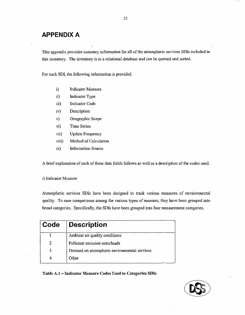
i) Indicator Measure
Atmospheric services SDIs have been designed to track various measures of environmental
quality. TO case comparisons among the various types of measure, they bave been grouped into
broad categories. Specitïcally, the SDIs bave been grouped into four measurement categories.
Code Description
Ambient air quality conditions
Pollutant emission rates/loads
Demand on atmospheric environmental services
Other
Table A.1 - Indicator Measure Codes Used to Categorize SDIs
32
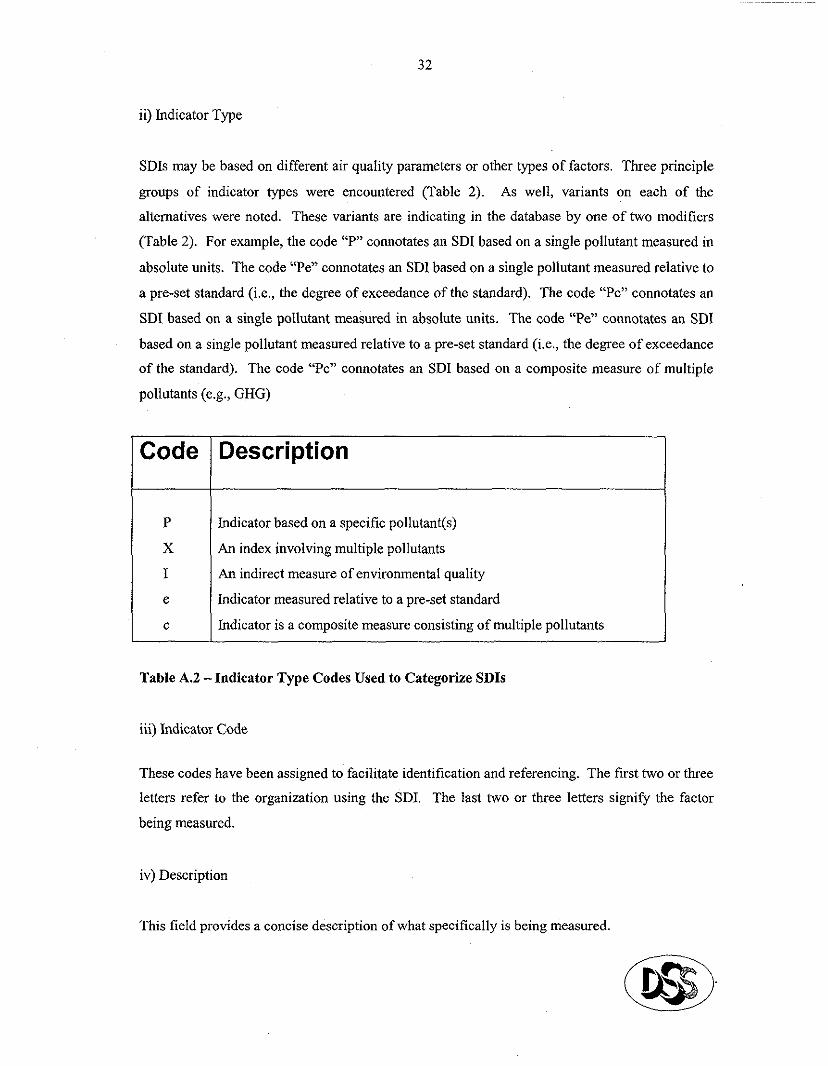
ii) Indicator Type
SDIs may be based on different air quality parameters or other types of factors. Three principle
groups of indicator types were encountered (Table 2). As well, variants on each of the alternatives were noted. These variants are indicating in the database by one of hvo modifiers
(Table 2). For example, the code ‘Y connotates an SDI based on a single pollutant measured in
absolute units. The code “Pe” connotates an SDI based on a single pollutant measured relative to
a pre-set standard (Le., the degree of exceedance of the standard). The code “Pc” connotates an
SDI based on a single pollutant measured in absolute units. The code “Pe” connotates an SDI
based on a single pollutant measured relative to a pre-set standard (i.e., the degee of exceedance
of the standard). The code “Pc” connotates an SDI based on a composite measure of multiple
pollutants (e.g., GHG)
Code Description
P Indicator based on a specific pollutant(s)
X An index involving multiple pollutants
1 An indirect measure of environmental quality
e Indicator measured relative to a pre-set standard
c Indicator is a composite measure consisting of multiple pollutants
Table A.2 - Indicator Type Codes Used to Categorize SDIs
iii) Indicator Code
These codes have been assigned to facilitate identification and referencing. The tïrst two or three letters refer to the organization using the SDI. The last two or three letters signify the factor
being measured.
iv) Description
This field provides a concise description of what specifïcally is being measured.
33
v) Responsible Organization
Each SDI has been proposed and/or developed and maintained by a particular organization. In some cases, the responsible organization is different than the organization that collects
monitoring data used to calculate SDI values.
vi) Geographic Scope
Each SDI pertains to a specific area as indicated in this field. Some indicators bave been
proposed for general use but are net being practically applied at the present time. In these cases,
the intended scale and scope of appl,ication is indicated as being “ns” (Le., net specifïed).
vii) Time Series
A key feature of SDIs is to track changes over time. This field provides information on the
period over which data have been used to calculate SDI values. Information is also included
regarding any key specifics conceming the supporting data set.
viii) Update Frequency
SDI values may change over time. This field provides information on how regularly monitoring
data are collected and new SDI values are calculated.
ix) Method of Calculation
This fïeld describes the salient features of the method used to calculate SDI values. Details are
provided which may affect the reliability and interpretation of SDI values. In some cases, details
on the calculation method may not be currently available or bave net been fully formulated. These records are denoted by “ns” followed by our best interpretation as to how reasonable
values for the SDI could be calculated.
34
x) Source
The large majority of atmospheric services SDI information is available through the Internet.
This field provides one or two Internet addresses from which the data used for the record were
primarily obtained and from which further details are available.
xi) Contents Summary
Table A.3* provides an overview of the types of pollutants that are used to track air quality in
various Canadian jurisdictions. Al1 of these different combinations of pollutants, at least in
theory, could be used to develop a comprehensive atmospheric services SDI at a national level.
Details for each of these indicators are provided in the more detailed tables in Appendix B.
a The acronyns used in this table are defined in the list of acronyms.
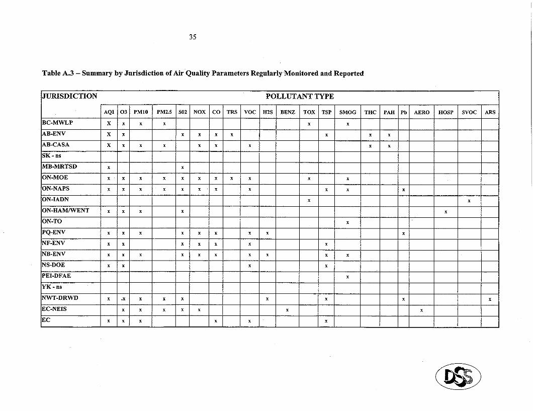
I I I l I I I I I I I I I I I I*I I
36
APPENDIX B
Summary Tables
For
Individual Atmospheric Services SDIS
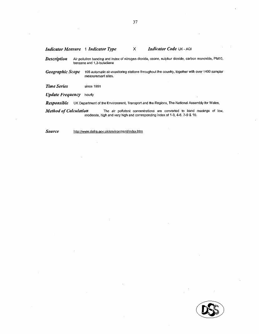
37
Indicator Measure 1 Indicator Type x Indicator Code UK - AQI
Description Air pollution banding and index of nitrogen dioxide. ozone. sulphur dioxide. caban monoxide, PM10, benzene and 1.3.buiadiene
Geographic SCOpe 108 automatic air-monitoring stations throughout the country, together with over 1400 sampler measurement sites.
Time Series sine 1991
Update Frequency hourly
Responsible UK Department of the Environment, Transport and the Regions. The National Assembty for Wales.
Method of Calculation The air poflutant concentrations are cawxted to band readings ai tow. moderate, high and very high and corresponding index of 1-3, 4-6. 7-9 & 10.
Source http://~.defra.~ov.uklenvironment/index.htm
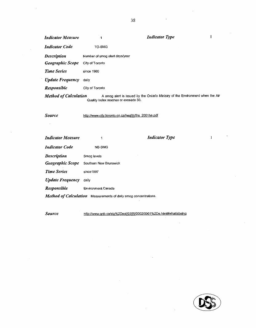
38
Indicator Measure 1
Indicator Code TO-SMG
Description Number Of smog ah?* dayslyear Geographic Scope C%Y of Toronto
Time Series since 1980
bdicator Type I
Update Frequency daily
Responsible City of Toronto
Method of Calculation A smog alert is issued by the Ontario Minisiry of lhe Environment when the Air Quality Index reaches or exceeds 50.
Source hlto:ll~.cihl.toronto.on.ca/health(ths 2001he.Ddf
Indicator Measure 1 Indicator Type
Indicator Code NB-SMG
Description smog kv‘A?. Geographic Scope Southem New Brunswick
Tinte Series since1997
Update Frequency daily
Responsible Environment Canada
Method of Calculation ~easuremenk of daily smo9 concentrations.
Source
I
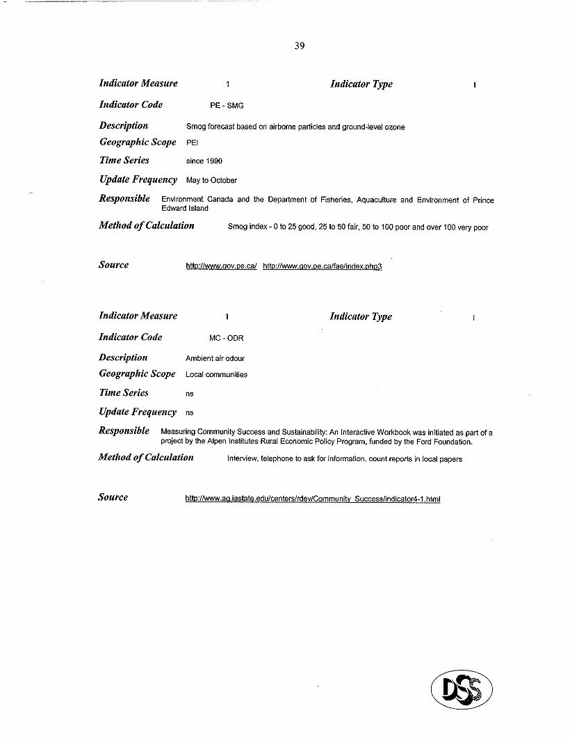
39
Indicator Measure Indicator Type I
Indicator Code PE - SMG
Description Smog forecast based on airborne particles and ground-level ozone
Geographic Scope PEI
Time Series since 1990
Update Frequetccy Zay to October
Responsible Environment Canada and the Depatiment of Fisheries, Aquaculture and Environment of Prince Edward Island
Method of Calculation Smog index - 0 to 25 good, 25 10 50 fair. 50 ta 100 poor and over 100 very poor
Source http:IIw.qw.pe.ca/ http://WWW.qov.pe.ca/fae/index.php3
Indicator Measure 1 Indicator Type I
Indicator Code MC ODR
Description Ambient air odour
Geographic Scope LO~~I canmunities
Time Series ns
Update Frequency ns
Responsible Measuring Community Sucu?ss and Sustainability: An Interactive Worhbooh was initiated as part of a project by the Alpen Institutes Rural Ewnomic Policy Program. funded by the Ford Foundation.
Method of Calculation Interview. telephone to ask for information, count reports in local papers
Source http://www.aa.iastate.edul~nters/rdevlCommunity Success/indicator4-l.html
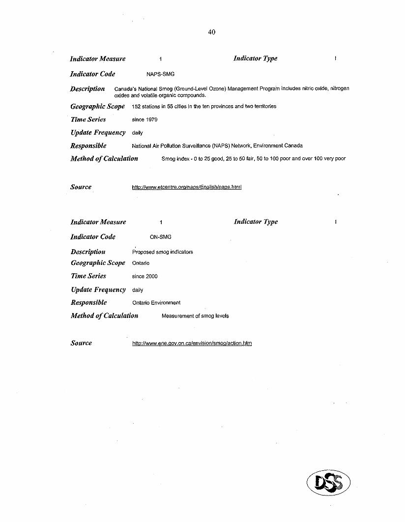
40
Zndicator Measure 1 Zndicator Type I
Zndicator Code NAPS-SMG
Description Canada% National Smog (Ground-Level Ozone) Management Program inctudes nitric oxide. nitrogen aides and volatile organic compounds.
Geographic Ecope 152 stations in 55 cities in the ten provinces and two territories
Time Series since 1979
Update Frequency daity
Responsible National Air Pottutton Surveillance (NAPS) Netwrk. Environ!nent Canada
Method of Calculation Smog index - 0 to 25 good, 25 to 50 faf. 50 to 100 poor and over 100 vety poor
Zndicator Measure 1 Zndicator Type t
Zndicator Code ON-SMG
Description Proposed smog indicators
Geographic Scope Ontario
Tinte Series sine 2000
Update Frequency daily
Responsible Ontario Environment
Method of Calculation Measurement of *mg tevets
Source httQ:llwww.e~e.aov.on.calenvisionlsmoq/ctio~.htm
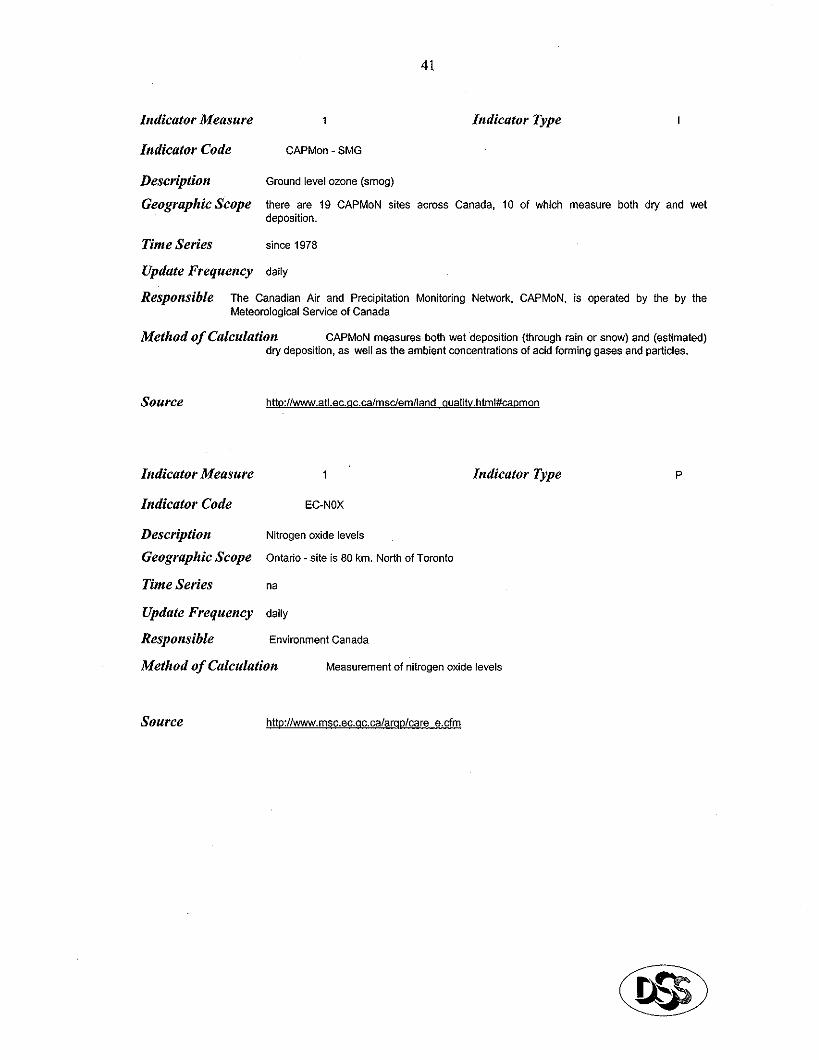
41
Indicator Me~sure 1 Indicntor Type
Indicator Code CAPMon - SMG
Description Ground level ozone (smog)
GeographicSCOpe there are 19 CAPMoN sites across Canada, 10 of which measure bath dry and wet deposition.
Tinte Series since 1978
Update Frequency daily
Responsible The Canadian Air and Precipitalion Monitoring Network, CAPMoN. is operated by the by the Meteorological Service of Canada
Method of Calculation CAPMoN measures both wet deposition (through min or snow) and (estimated) dry deposition, as well as the ambient concentrations of acid forming gases and pa!Wes.
Source httQ:l/www.atl.ec.ac.ca/msc/emlland aualitv.html#caQmon
Indicator Measure 1
Indicator Code EC-NOX
Description Nitrogen oxide levels
Geographic SCOpe Ontario-site is 80 km. North of Toronto
Time Series na
Update Frequency daily
Responsible Environment Canada
Method of Calculation Measurement of nitmgen oxide levels
Source httQ:II~.msc.ec.ac.calar~Ql~re e.cfm
P
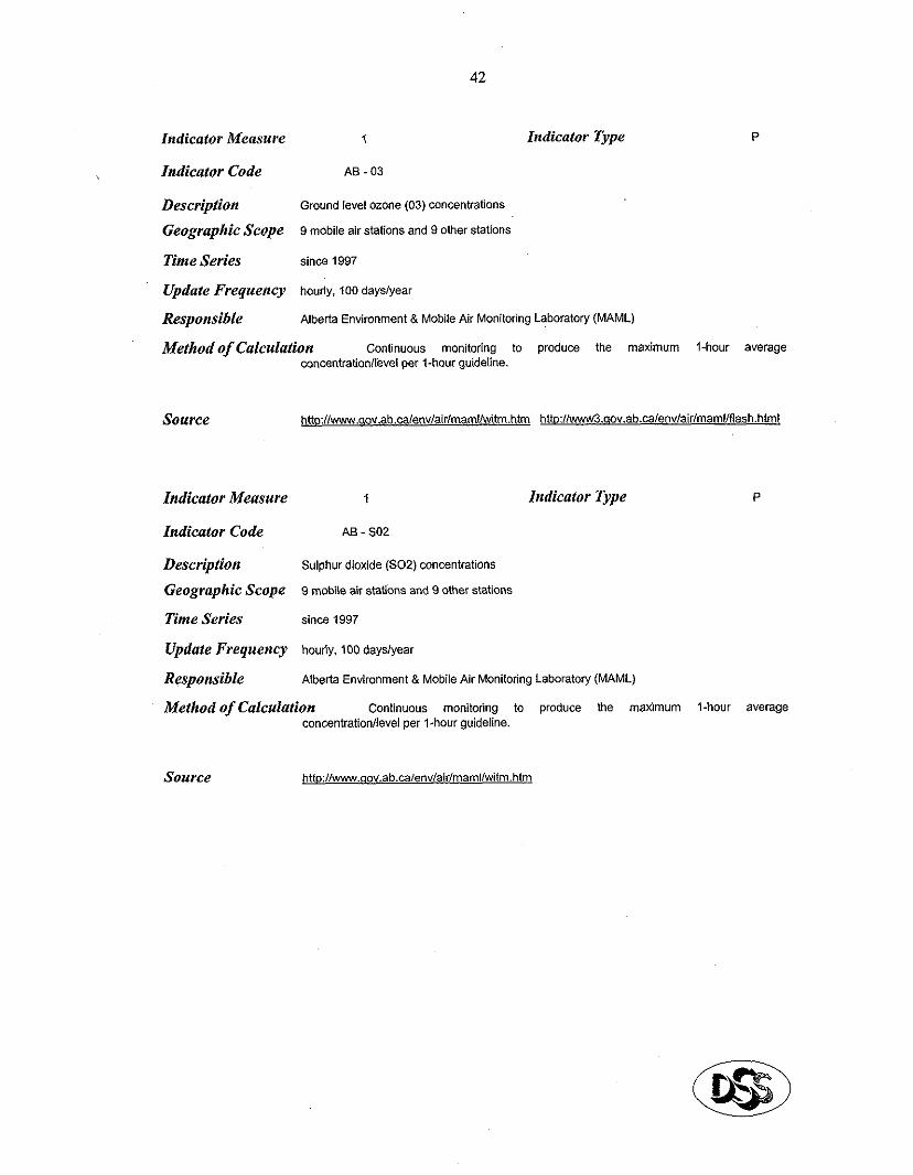
42
Indicator Type Indicator Measure 1 P
Indicator Code AS-03
Description Ground level ozone (03) concentrations
Geographic Scope 9 mobile air stations and 9 other stations
Time Series since 1997
Update Frequency hourly, 100 dayslyear
Resporsible Alberta Environment & Mobile Air Monitoring laboratory (MAML)
Method of Calculation ConBnuous monitoring to Qrcduce the maximum l-heur average concentrattonltbvet per l-hou guideline.
Source h~~:lI~.~ov.ab.~lealenv/airlmaml/witm.h~ ht~:l/www3.sov.ab.ca/envlairlmamllflash.html
Indicator Measure 1 Indicator Type P
Indicator Code As-SO2
Description Sulphur dioxide (SOZ) concentrations
Geographic Scope 9 mobile air stations and 9 other stations
Time Series since 1997
Update Frequency hourly. 100 dayslyear
Responsible Alberta Environment & Mobile Air Monitoring Laboratory (MAML)
Method of Calculation Continuous monitoring to produce the maximum I-hou average concentrationllevel per l-hou guideline.
Source
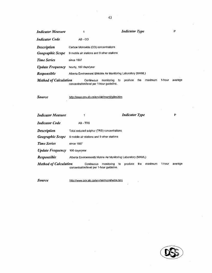
Indicator Measure 1
Indicator Code AS-CO
43
Indicator Type P
Description Carbon Monoxide (CO) concentrations
Geographic Scope 9 mobile air stations and 9 olher stations
Tinte Series since 1997
Update Frequency hourly. 100 dayslyear
Responsible Alberta Environment &Mobile Air Monitoring Laboratory (MAML)
Method of Calculation Continuous monitoring to produce the maximum l-hou average concentrationilevel per 1.heur guideline.
Source hd~:/lwwvY.~ov.ab.calenvlairlmaml/witm.htm
Indicaior Measure 1 Indicator Type P
Indicator Code AS - TRS
Description Total reduced sulphur (TRS) concenbations
Geographic Scope 9 mobile air stations and 9 other stations
Tinte Series since 1997
Update Frequency 100 dayslyear
Responsible Alberta Environment& Mobile Air Monitoring Laboraloly (MAML)
Method of Calculation Continuous monitoring to produce lhe maximum l-hou average concentrationllevel per 1.heur guideline.
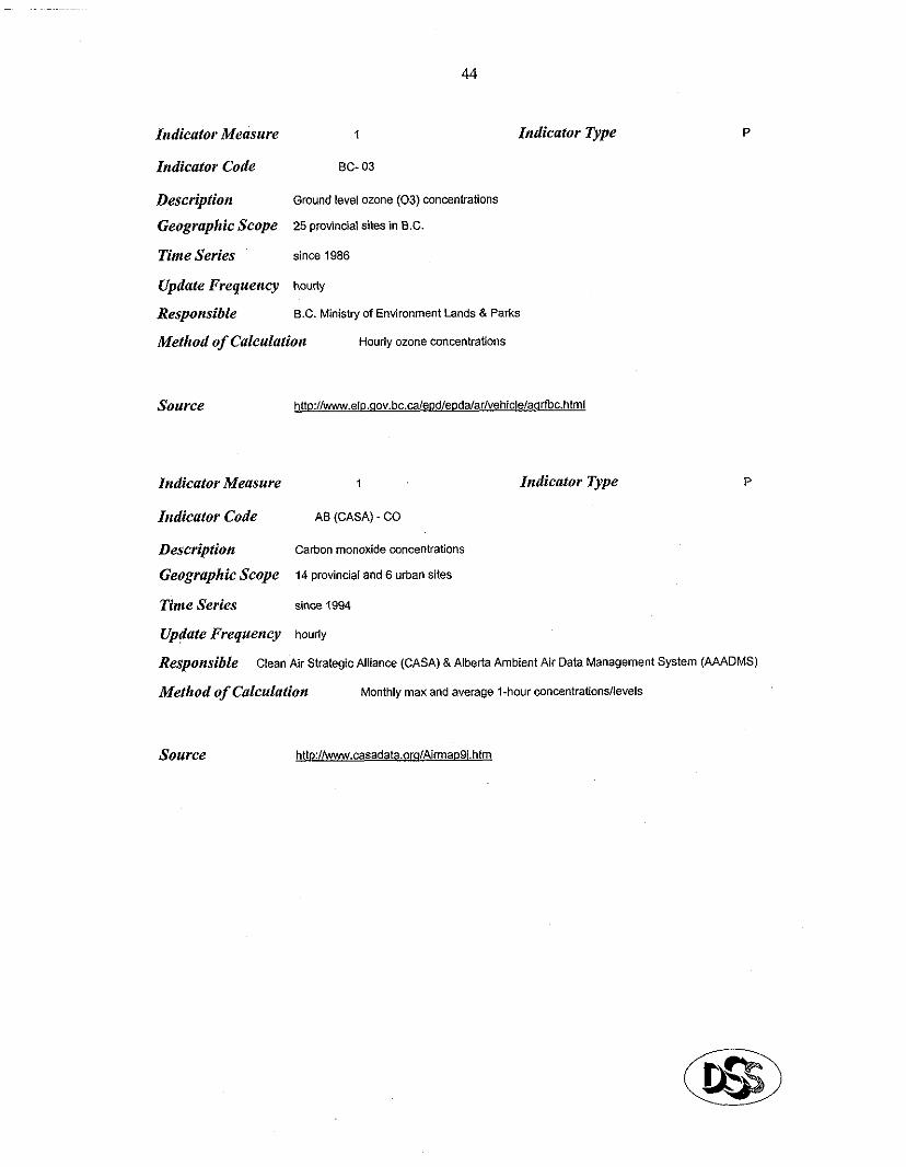
44
Indicator Type Indicator Measure 1
Indicator Code BC- 03
Description Ground kvel ozone (03) concentrations
Geograpbic Ecope 25 provincial sites in B.G.
Tinte Series sine 1986
Update Frequency hourly
Responsible 0.C. Ministry of Environment Lands & Parks
Method of Calculation Hourly ozone concentrations
Source hnp:llwww.elp.aov.bc.ca/epdlepda/ar/vehiclelaa~c.hlm~
P
P Indicator Measure 1 Indicator Type
Indicator Code AB (CASA) CO
Description Carbon monoxide concentrations
Geographic Scope 14 provincial and 6 urban sites
Tinte Series since 1994
UP-te Frequency houdy
Responsible Clean Air Strategic Alliance (CASA) & Alberta Ambient Air Data Management System (AAADMS)
Method of Calculation Monthly max and average l-hou cnncentrationsllevels
Source
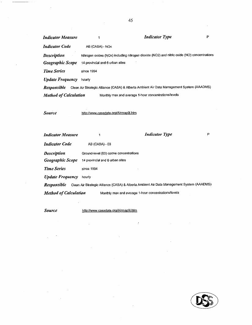
45
Indicator Measure 1 Indicator Type P
Indicator Code AS (CASA) - NOY.
Description Nitrogen oxides (NOx) including nitrogen dioxide (NEZ) and nitric oxide (NO) concentrations
Geographic Scope 14 provincial and 6 utban sites
Time Series since 1994
Update Frequency houdy
Responsible Clean Air Strategic Alliance (CASA) 8 Alberta Ambient Air Data Management System (AAADMS)
Method of Calculation Monthly max and average 1.heur ConcentrationsIlevek
Source http:llw.casadata.or~lAirmaDSi.htm
Indicator Measure 1 Indicator Type P
Indicator Code AS (CASA) - 03
Description Ground-level(O3) ozone concentrations
Geographic Scope 14 provincial and 6 urban sites
Time Series since 1994
Update Frequency hourly
Responsible Clean Air Strategic Alliance (CASA) & Alberta Ambient Air Data Management System (AAADMS)
Method of Calculation Monthly max and average l-hou concentrationsllevels
Source
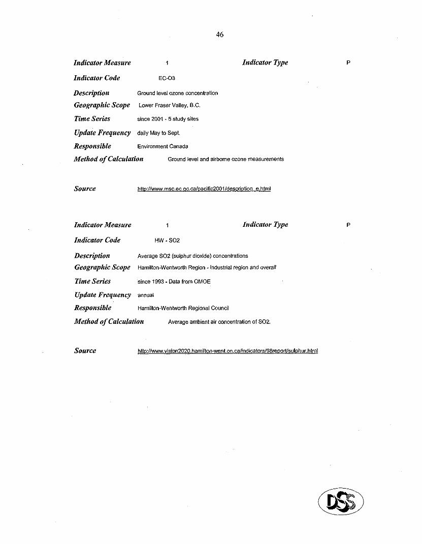
46
Indicator Meusure 1 Indicator Type
Indicator Code EC-03
Description Ground level ozone concentration
Geographic Scope Lower Fraser Valley, S.C.
Tinte Series sine 2001 - 5 study sites
Update Frequency daily May to Sept.
Responsibie Environment Canada
Method qf Calculation Ground le’4 and airbome ozone measurements
Source http:II~.msc.ec.ac.~lpa~~c2OOl/descdption ehtml
Indicator Measure 1 Indicator Type
Indicator Code HW - SO2
Description Average SO2 (sulphur dioxide) concentrations
Geographic Scope Hamilton-Wentworth Region - industrial region and overall
Time Series since 1993 - Data from OMOE
Update Frequency annua~
Responsible Hamilton-Wentworth Regional Council
Method of Calculation Average ambient air concentration of S02.
Source
P
P
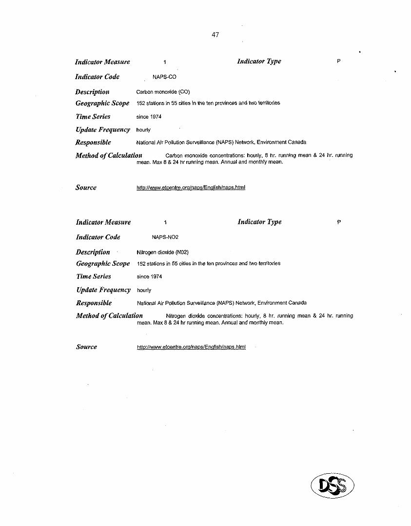
47
Indicator Type P Indicator Measure 1
Indicator Code NAPS-CO
Description Carbon monoxide (CO)
Geographic Scope 152 stations in 55 cities in the te” provinces and tvo territories
Time Series since 1974
Update Frequency hourly
Responsibte National Air Pollution Surveillance (NAPS) Network, Environment Canada
Method of Calculation Cart~on monoxide concentrations: haurly, 8 hr. running mean & 24 hr. running mean. Max 8 & 24 hr running mean. Annual and monthly mean.
Source http:/l~.etcentre.orq/naos/Enalish/naDs.html
Indicaior Measure
Indicator Code
Description Geographic Scope
Time Series
Update Frequency
Responsible
1 Zndicator Type
NAPS-NO2
Nitrogen dioxide (N02)
152 stations in 55 cities in the ten provinces and two territories
since 1974
hourly
National Air Pollution Surveillance (NAPS) Nehvork. Environment Canada
Method of Calculation Nitrogen dioxide concentrations: hourly. 8 hr. running mean & 24 hr. running maan. Max 0 & 24 hr running mean. Annual and monthly mean.
SOUtVX?
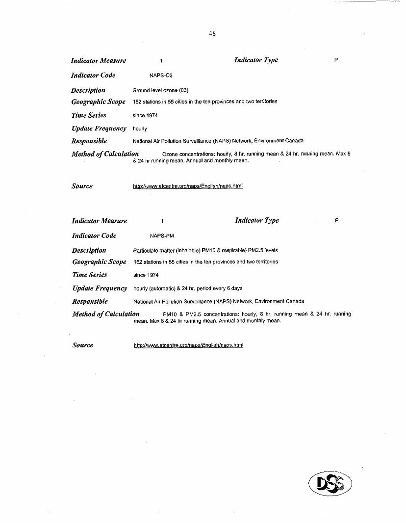
48
Indicator Measure 1
Indicator Code NAPS-03
Indicator Type P
Description Groundlevelozone(03)
Geographic Scope 152 stations in SS cities in the ten provinces and two territodes
Time Series since 1974
Update Frequency hourly
Responsible National Air Pollution Surveillance (NAPS) Netwrk, Environment Canada
Method of Calculation Ozone concentrations: hourly. 8 hr. running mean 8 24 hr. running mean. Max 8 8 24 hr running msan. Annuat and monlhly mean.
Source
Indicator Measure 1 Indicator Type P
Indicator Code NAPS-PM
Description Particulate matter (inhalabk?) PM10 &‘respirable) PM25 levels
Geographic Scope 152 stations in 55 chies in the ten provinces and two terdtories
Tinte Series since 1974
Update Frequency houdy (automatic) & 24 hr. period every 6 days
Responsible National Air Pollution Surveillance (NAPS) Netwrk, Environment Canada
Method of Calculation PM10 8. PM25 concentrations: hourly. 0 hr. running mean & 24 hr. running mean. Max,S & 24 hr running mean. Annual and monthly mean.
Source
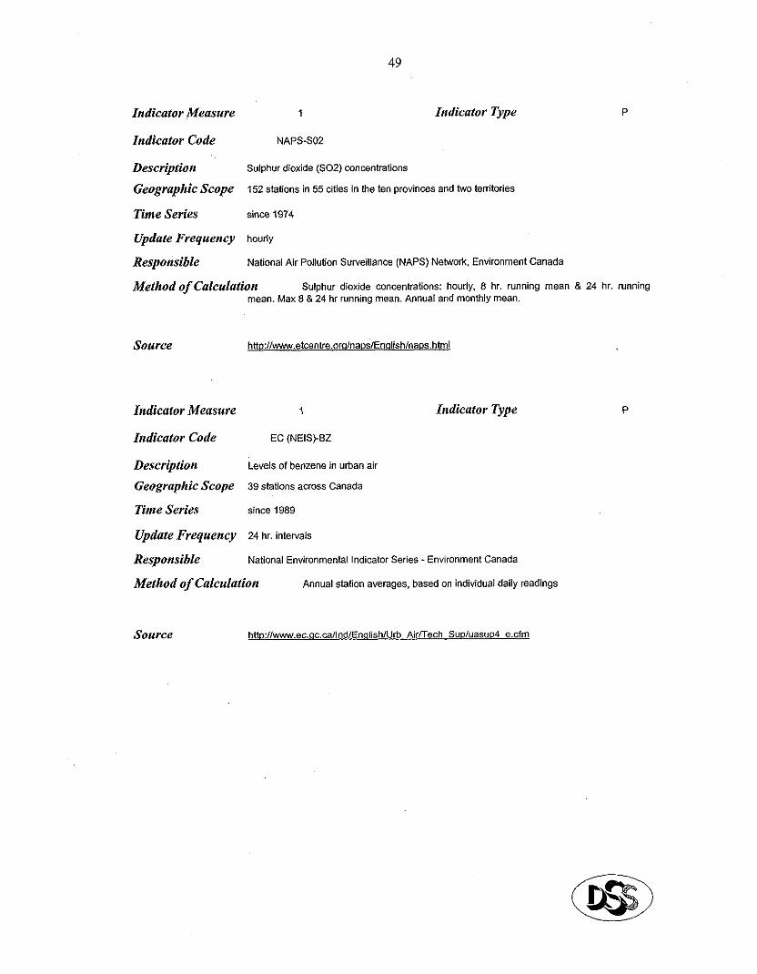
49
Indicator &feasure 1 Indicator Type P
Indicator Code NAPS-SO2
Description Sulphur dioxide (SOZ) concentrations
Geographic Scope 152 stations in 55 Mies in the ten provinces and two temitories
Time Series since 1974
Update Frequency hourly
Responsible National Air Pollution Surveillance (NAPS) Network. Environment Canada
Method of Calculation Sulphur dioxide concentrations: hourly. 8 hr. running mean & 24 hr. running mean. Max 8 & 24 hr running mean. Annual and monthly mean.
Source htt~:l/www.etcentre.orql~a~slEn~lish/na~s.html
Zndicator Measure 1 Zndicator Type
hdicator Code EC (NEWEIZ
Description Levels of benzene in urban air
Geographic Scope 39 stations across Canada
Tioze Series sine 1989
Update Frequency 24 hr. intervals
Responsible National Environmental Indicator Series - Environment Canada
Method of Calculation An~al station averages, based on individual daily readings
P
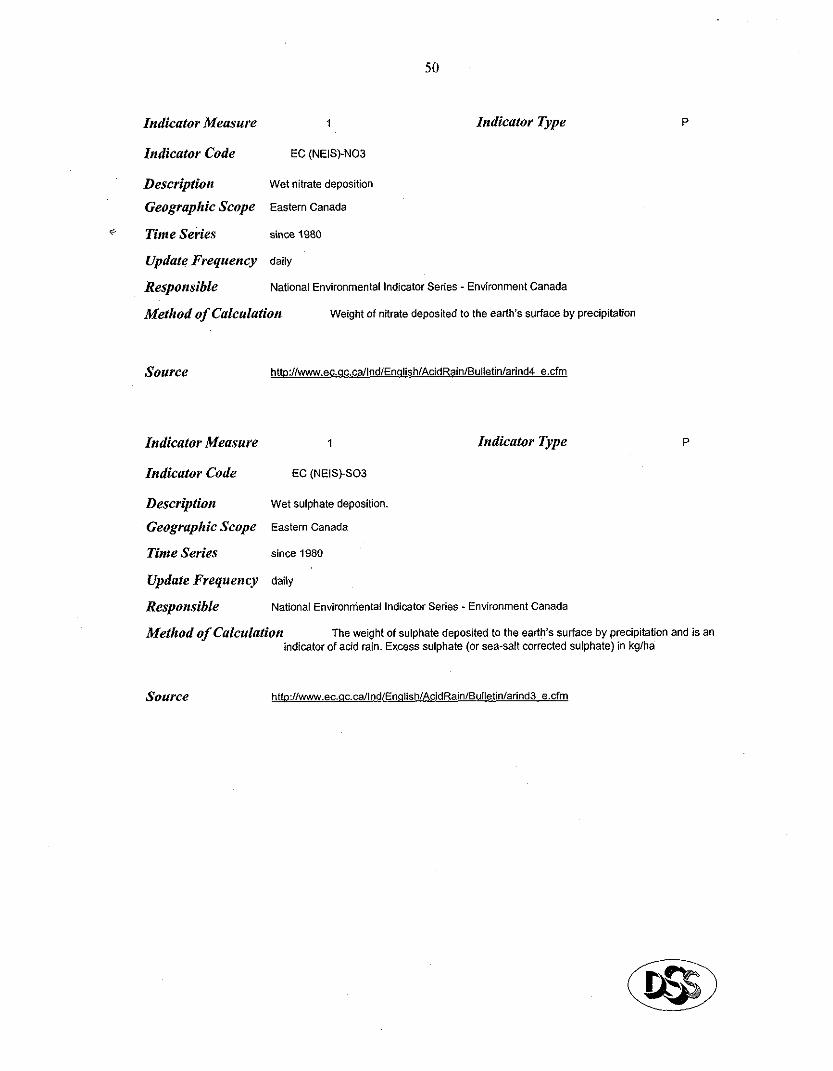
50
Indicator Measure 1 Indicator Type
Indicator Code EC (NEW-NO3
Description Wet nitrate deposition
Geographic Ecope Eastern Canada
Time Series since 1980
Update Frequency daity
Responsible Natlonal Environmental Indicator Series - Environment Canada
Method of Calculation Weight of nitrate deposited to the earth’s surface by Qrecipitation
P
Source htt~://www.ec.~c.ca/Ind/En~lishlAcidRain~Sul~etinlarind4 e.cfm
Indicator Measure 1 Indicator Type P
Indicator Code EC (NEW.503
Description Wet sulphata deposition.
Geographic Scope Eastern Canada
Time Series since 1980
Update Frequency daily
Responsible National Environtiental Indicator Series - Environment Canada
Method of Calculation The weight of sulphate deposited to the earth’s surface by Qrecipitation and is an indicator of acid min. Excess sulphate (or sea-Salt corrected sulphate) in kg/ha
source htt~://www.ec.~c.calIndlEnqlish/AcidRainl~ulletinladnd3 e.cfm
51
Indicator Type Indicator M?asure 1
Indicator Code NB-CO
Description Carbon monoxide concentrations
Geographic Scope mainly southem New Brunswick and St. John’s
Time Series since 1979
Update Frequency daily
Responsible New Brunswick Environment
Method of Calculation Monthly max and mean concentrations
Source httD://www.4nb.ca/elu-ea1/0355/0003/0023-e.html
Indicator Measure 1 Indicator Type
Indicator Code NB - H2S
Description Hydrogen sulphide concentrations
Geographic Scope mainty southem New Brunswick and St. John%
Tinte Series since 1979
Update Frequency daily
Responsible New Brunswick Environment
Method of Calculation Monthly average concentration
Source
Indicator Meusure 1
Indicator Code NB - NOx
52
Indicator Type
Descriptiott Nitrous oxide concentrations
Geographic Scope mainly southem New Brunswick and St. John%
Time Series since 1979
Update Frequency daily
Responsible New Brunswick Environment
Method of Calculation Monthly max and mean concentrations
Source ht$:/iwww.~nb.ca/el~-ea1/0355/0003/0023-e.ht~l
Indicator Measure 1 Odicator Type
Indicator Code NB - SO2
Description Sulphur dioxide concentrations
Geographic Scope mainly southsm New Brunswick and St. John%
Time Series since 1979
Update Frequency daily
Responsible New Brunswick Environment
Method of Calculatioa Monthly max and mean concentrations
Source
53
Indicator Type Indicator Measure 1
Indicator Code NB-PM
Description Particulate matter PM10 levels
Geographic Scope New Brunswick
Time Series since 1994
Update Frequency once ever~ 6 days
Respoasible New Brunswick Environment
Method of Calculation Measurement of monthty average PM-10 tevels
P
Source htt~:llwww.~nb.caletao~2D~~llO35510008100Ol-e.html
Indicator Measure 1 Indicator Type
Indicator Code NF-CO
Description Carbon monouide tevets
Geographic Scope Newfoundland
Time Series sine 1999
Update Frequency hourty
Resporrsible Netioundland Environment in wnjunction with tbe National Air Pollution Surveillance (NAPS)
Method of Calculation Carbon monoxide levels
Source
54
Indicator Type Indicator Measure 1 P
Indicator Code NF-NOX
Description Nitrous oxide levels
Geographic Scope Netioundland
Time Series since 1999
Update Frequency houdy
Responsible Newfoundtand Environment in conjunciion with the National Air Pollution Surveillance (NAPS)
Method of Calculation Nitrous oxide levels
Source htt~:llwww.qov.nf.ca/env/envloollDrevlenvironmenial%5Fscience.as~
P Indicator Measure 1 Indicator Type
Indicator Code NF-03
Description Ground level ozone levels
Geographic Scope Netioundland
Tinte Series sine 1987
Update Frequency hourly
Responsible Newfoundland Environment in coniunction wilh the National Air Pollution Surveillance (NAPS)
Method of Calculution Ground level ozone levels
Source htt~:/l~.aov.nf.ca/env/EnvlPollPrev/environmen~l scienceas
55
Indicator Measure 1 Indicator Type P
Indicator Code NF-SO2
Description Sulfur dioxide levels
Geographic Scope Netioundland
Time Series sine 1999
Update Frequemy hourly
Responsible Newfoundland Environment in conjunction with the National Air Pollution Surveillance (NAPS)
Method of Calculation Sulphur dioxide levels
Source httQ:ll~.~ov.nf.ca/env/envl~ol~Qfevienvir~nmental%5F~cien~.asQ
Indicator Measure 1 Indicator Type
Indicator Code NF-SO3
Description Wet sulQhale k?Ws
Geographic Scope Newfoundland - 5 sites
Time Series since 1983
P
Update Frequency week~y
Responsible Netioundland Environment Precipitalion Monitoring Nebvxk (NEPMoN))
Method of Calculation The weekly wet-only precipitation data irom these stations Will be used to complement the daily data collected by Environment Canada’s Canadian Air and Precipitation Moniloring Network (CAPMoN)
Source httQ://www.aov.nf.calenv/env/pollQrevlacid min Qrwram dwt of &SD
56
Indicator Measure 1 Indicator Type
Indicator Code NS -03
Description Gvxmd level ozone concentrations
Geographic Scope 10 stations wxm NOV~ Su%a
Time Series since 1986
Update Frequency hourly
Responsible Nom Scotia Dept. of the Environment
Method of Calculation Number of one-hou exceedances of ground bel 0Z0W
Source htlp:llwvvur.~ov.ns.calenvilSoerlenvdoc.pdf
Indicator Measure 1 Indicator Type
Indicator Code NS-SO3
Description Sulphate deposition
Geographic Scope 10 stations across Nova Scotia
Time Series since 1978
Update Frequency week~y
Responsible Nova SC& Dept. of the Environment
Method of Calculation Annual sulphate deposition exceedance
Source http://www.aov.ns.ca/envi/Soer/envdoc.odf
P
57
Indicator Measure 1 Indicator Type
Indicator Code NT-03
Description Ground level ozone levels
Geographic Scope ‘fellovdmife
Tinte Series sine 1998
Update Frequency hourly
Responsible NWT Dept. of Resources, Wildlife & Economie Development (RWED)
Method of Calculation Monthly average and hourly max concentrations
P
Source htto://www.~ov.nt.calRWEDle~sl~dfslQQ-OONWT Air Qualitvndf
Indicator Measure 1 Indicator Type
Indicator Code N-f - Ars
Description Arsenic levek.
Geographic Scope yeknvknife
Time Series sine 1994
Update Frequency 24 hr. intewats
Responsible NWT Dept. of Resources, Wildlife & Economie Development (RWED)
Method of Calculation Annual and 24 hr max levels collected from 53 samples
P
Source httr>://www,aov,nt,c/RWED/eos/~dfs/99-OONWT Air Qualitudf
58
Indicator Type Indicator Measure 1
Indicator Code NT - H2S
Description Hydrogen sulphide levels
Geographic Scope Yellowknife
Tinte Series since 2000
Vpdate Frequency hourly
Responsible NWT Dept. of Resources, Wildlife 8 Economie Development (RWED)
Method of Calculation Exceedance of hourly and 24 hr. averages
P
Source http://w.aov.nt.ca/RWED/eps/pdfs/99-OONWT Air Qualitvadf
Indicator Measure 1 Indicator Type
Indicator Code M-NO3
Description Nitrate deposition levels
Geographic Scope Yellowknife
Time Series since 1985
Update Frequency daily
ResponsibIe NWT Dept. of Resources. Wildlife & Economie Development (RWED)
Method of Calculation Annual deposition rate
Source htto:/lw.aov.nt.ca/RWED/epslpdfsl99-OONWT Air Quality.pdf
59
Indicator Measure 1 Indicator Type
Indicator Code NT-Pb
Description Lead levels
Geographic Scope Yellowknife
Tinte Series since 1992
Update Frequency 24 hr. intervals
Responsible NWT Dept. of Resources. Wildlife & Ewnomic Development (RWED)
Method of Calculalion Annval and 24hr max levels wllected from 53 samples
Source http://w.aov.nt.ca/RWED/eps/pdfs/99-OONWT Air Qualitv.pdf
Indicator Measure 1 Indicator Type
Indicator Code NT SO3
Description Sulphate deposition levels
Geographic Scope Yellowknife
Tinte Series since 1985
Update Frequency daily
Responsible NWT Dept. of Resources. Wildlife & Ewnomic Development (RWED)
Method of Calculation Annual avera9es of sulphate levels
Source htto:/hvww.~ov.nt.ca/RWED/ePslpdfs/99-OONWT Air Qualitudf
P
P
60
Indicator Measure 1 Indicator Type
Indicator Code ON-03
Description concentrations of ground levd ozone (03)
Geographic Scope 38 sites in 1998
Time Series since 1971
Update Frequency hourly
Responsible Ontario Minisby of the Environment
Method of Calculalion Continuous monitoring to produce the maximum l-heur concenlrationllevel per l-hou guideline. Number of ozone exceedance days
Source h~p:llwww.ene.~ov.on.ca/envisionltechdo~l4054e.odf
Indicator Measure 1 Indicator Type
Indicator Code PQ-Pb
Description Lead (Pb) concentrations
Geographic Scope Quebec
Time Series since 1975
Update Frequency ns
Responsible Qu6bec Environnement
Method of Calculation Annual mean lead concentrations
P
P
61
Indicafor Me~sure 1 Indicator Type P
Indicator Code UK-03
Description Grand level ozone (03) uxxentrations
Geographic ScOpe 108 automatic air-monitoring stations ttvoughout the country. together with over 1400 sampler measurement sites.
Tinte Series since 1973
Update Frequency real time automatic measurements
Responsible UK Department of the Environment, Transport and the Regions, The National Assembly for Wates.
Method of Calculation 8 hourty or houdy mean. Number of days of exceedance.
Source htt~:llwww.aeat.w.uklnetcen/rer>ort96lindex.html
Indicator Measure 1 Indicator Type P
Indicator Code UK - BEN2
Description Benzene concentrations
Geographic Scope 108 automatic air-monitoring stations throughout the country, together with ow 1400 sampler measurement sites.
Time Series since 1996
Update Frequency houdy
Responsible UK Department of the Environment. Transpod and the Regions. The National Assembty for Wates,
Method of Calculation Annuat mean concentrations of benzene
Source
62
Indicator Measure 1
Indicator Code UK - NO3
Indicator Type P
Description Wel nitrate (N03) deposilion
Geographic Scope 108 automatic air-monitaring stations throughout the country. together with over 1400 sampler measurement sites.
Time Series since 1986
Update Frequency daily & weekly
Responsible UK Department of the Environment, Transport and the Regions, The National Assembly for Wales,
Method of Calculation Daily, weekly and monthly concentrations of wet nitrate
Source htt~:l/www.defra.aov.uklenvironmenVindex.htm
Indicator Measure 1 Indicator Type P
Indicator Code UK - SO3
Description Wet sulphate (SO3) deposition
Geographic SCOp.? 108 automaiic air-monitoring stations throughout the counby, together with over 1400 sampler measurement sites.
Tinte Series since 1986
Update Frequency daily 8 weekly
Responsible UK Department of the Environment. Transport and the Regions, The National Assembly for Wales,
Method of Calculation Daily, weekly and monthly concentrations of wet sulphate
Source
63
Indicator Measure 1
Indicator Code WA-03
Description Ground level ozone (03) levels
Geographic Scope Washington
Tinte Series since 2001 - 9 sites
Indicator Type P
Update Frequency 1 hr.aver.8hr.aver.
Responsible Washington Dept. of Ecdogy
Method of Calculation Ground level ozone tevels
Source http:/lairr.ecv.wa.aovlPubliclaqn.html
Indicator Measure 1 Indicator Type PC
Indicator Code AB - NOx
Description Nitrogen oxides (NOx) induding nitrogen dioxide (N02) and nittic oxide (NO) concentrations
Geographic Scope 9 mobite air stations and 9 other stations
Tinte Series since 1997
Update Frequency hourly. 100 daysiyear
Responsible Alberta Environment &Mobile Air Monitoring Laboratory (MAML)
Method of Calculatioa Continuous monitoting to produce the maximum l-heur avwage concentrationllevel per l-heur guideline.
Source
64
Indicator Measure 1 Indicator Type
Indicator Code AB - PAH
Description Polycyclic aromatic hydrocarbons (PAH) levels
Geographic Scope 9 mobile air stations and 9 stations
Tinte Series since 1997
Update Frequency 100 dayslyear
Responsible Alberta Environment& Mobile Air Monitoring Laboralory (MAN)
Method of Calculation Continuous monitoring to produce the maximuw l-hou concentrationllevel per l-heur guideline.
PC
Indicator Measure 1 Indicator Type PC
Indicator Code AI3 - THC
Description Total hydrocwbons (THC) comprised of methane (CH4) and reactive hydrocarbons (RHC)
Geographic Scope 9 mobile air stations and 9 stations
Tinte Series since 1997
Update Frequency 100 dayslyear
Responsible Alberta Environment& Mobile Air Monitoring Laboratory (MAML)
Method of Calculation Continuous monitoring to produce the maximum 1-heur average mncentrationllevel per l-heur guideline.
65
Indicator Measure 1 Indicator Type PC
Indicator Code AS - TSP
Description Total suspended particulate (TSP) levels
Geographic Scope 9 mobile air stations and 9 other stations
Tinte Series since 1997
Update Frequency hourly
Responsible Alberta Environment& Mobile Air Monitoring Laboratory (MAML)
Method of Calculation Conlinuous monitoring to produce the maximum l-heur average concentrationllevel per l-hou guideline.
Source http:/l~.aov.ab.ca/env/airlmaml/witm.htm
Indicator Measure 1 Indicator Type PC
Indicator Code AS (CASA)- PAH
Description Polycyclic aromatic compounds (PAH) levels
Geographic Scope 14 provincial and 6 urban sites
Time Series since 1994
Update Frequency once evety 6 days
Responsible Clean Air Strategic Alliance (CASA) & Alberta Ambient Air Data Management System (AAADMS)
Method of Calculation Monthly daily average and max concentrations
Source
66
tndicator Type Indicator Measure 1 PC
Indicator Code AB (CASA) - PM
Description Particulate matter PMlO&PM2.5 levels
Geographic Scope 14 provincial and 6 urban sites
Time Series since 1994
Update Frequency hourly
Responsible Clan Air Strategic Alliance (CASA) & Alberta Ambient Air Data Management System (AAADMS)
Method of Calculation Monthty max and average l-hou wncentrationsllevels
Source httr):llwww.casadata.orq/AinapSi.htm
PC Indicator Measure 1 Indicator Type
Indicator Code AS (CASA) - VOC
Description Volatile organic cnmpound (VOC) concentrations
Geographic Scope 14 provincial and 6 urban sites
Time Series since 1994
Update Frequency once ewy 6 days
Responsible Clean Air Strategic Alliance (CASA) 8 Alberta Ambient Air Data Management System (AAADMS)
Method of Calculation Monthly max and average l-hour concentrationsltevels
Source
Indicator Measure 1 Indicator Type PC
Indicator Code AE (CASA) - THC
Description Total hydrocarbons (THC) levels comprised of methane (CH4) and reactive hydrocarbons (RHC)
Geographic Scope 14 provincial and 6 urban sites
Time Series *ince 1994
Update Frequency once ewy 6 days
Responsible Clean Air Strategic Alliance (CASA) & Alberta Ambient Air Data Management System (AAADMS)
Method of Calculation Monthly daily avecage and max concentrations
Indicator Measure I Indicator Type PC
Indicator Code EC-PM
Description Particulate matter PM concentrations
Geographic Scope Lover Fraser Valley. SC.
Time Series since 2001 -- 5 study sites
Update Frequency daily May Sept.
Respoasible Environment Canada
Method of Calculaiion Ground and airborne PM measurements
68
Indicator Me~sure 1
Indicator Code EGVOC
Description Volatile organic wmpounds levels
Geographic Scope Ontario site is 80 km. Noah of Toronto
Time Series unavailable
Update Frequency daily
Responsible Environment Canada
Method of Calculation Measurement of WC levels
Source htto:llwww.msc.ec.uc.calar4o/care e.cfm
Indicator Type
Indicator Measure 1 Indicator Type
Indicator Code EC-Ad
Description .4erosol levels Geographic Scope Ontario-site is 80 km. North of Toronto
Time Series ns
Update Frequency daily
Responsible Environment Canada
Method of Calculation tvteasurement Of aeroso\ lWBIS
PC
PC
69
Indicator Measure 1 Indicator Type
Indicator Code HW-PM
Description Average particulate matler PM10 concentrations
Geographic Scope Hamilton-Wentwxth Regioti - industdal region and overall
Tinte Series since 1993 -Data irom OMQE
PC
Update Frequency annual
Responsible Hamilton-Wentwwth Regional Council
Method of Calculation Average ambient air concentration of PMIO.
source htlp:/l~.vision202O.hamilton-went.on.~lindi~torsl98repo~pmlO.html
Indicator Measure 1 Indicator Type PC
Indicator Code IADN-TOX
Description PA&. PCB and organochlorine compounds (which~are all Semivolatile Qrganic Compounds)
Geographic .%Ope Great Lakes Basin in Canada and US.
Time Series sine 1990
Update Frequency ns
Responsible IADN (The Integrated Atmospheric Deposition Network). Environment Canada and EPA
Method of Calculation Measures PCB, PAH. SVOC and trace metal levels in air and precipitation (deposition)
Source h~p://WWW.msc.ec.ac.caliadnlindex e.html
70
Indicator Me~sure 1 Indicutor Type PC
Indicator Code MC-PM
Description High particulate matter PM days
Geographic Scope Boca communities
Tinte Series ns
Update Frequency ns
Responsible Measuring Community Success and Sustainabilily: An Interactive Workbooh was initiated as part a project by the Aspen Institut& Rural Economie Policy Program, funded by the Ford Foundation.
Method of Calculation Compare to level of Qarticulates irom local EPA office or weather service, on consistent sek?cted days annually
Source http:/l~.a~.iastate.edulcenterslrdevlCommuni~ Success/indicator4-1 .html
Indicator Measure 1 Indicator Type PC
Indicator Code NAPS-TSP
Description Total suspended particulates (TSP) levels
Geographic Scope 152 stations in 55 cities in the ten provinces and two territaies
Time Series since 1974
Update Frequency 24 hr. period evay 6 days
Responsible National Air Pollution Surveillance (NAPS) Network, Environment Canada
Method of Calculation 24 hr. concentrations of total suspended particulates
Source
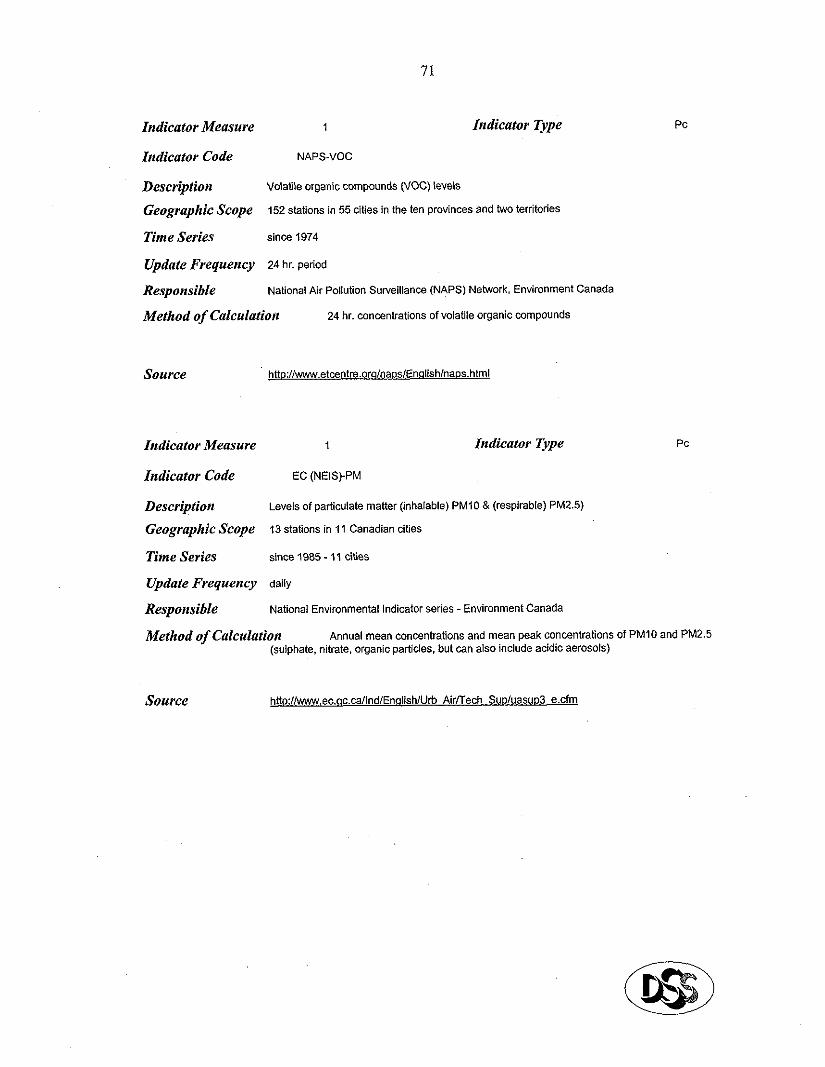
71
Indicator Measure 1 Indicator Type
Indicator Code NAPS-VOC
Description Volatile organic compounds (voc) level?.
Geographic Scope 152 stations in 55 cities in the ten provinces and two territories
Tinte Series since 1974
Update Frequency 24 hr. Qeriod
Responsible National Air Pollution Surveillance (NAPS) Network. Environment Canada
Method of Calculation 24 hr. concentrations of volatile organic compounds
Source http:liwww.etcentre.orqlnaps/En~lishl~aps.html
Indicator Measure
Indicator Code
Description Geographic Scope
Time Series
Update Frequency
Responsible
1
EC (NEIS).PM
Indicator Type
Levels of particulate matter (inhalable) PM10 & (respirable) PM2.5)
13 stations in 11 Canadian cilies
since 1985 - Il cities
daily
National Environmental Indicator series - Environment Canada
PC
PC
Method of Calculation Annual mean concentrations and mean peak concentrations of PM10 and PM2.5 (sulphate, nitrate. organic particles. but cari also include acidic aerosols)
Source hno://www.ec.ac.ca/lnd/Enalish/U~ Air/Tech Su~/uasuQ3 e.cfm
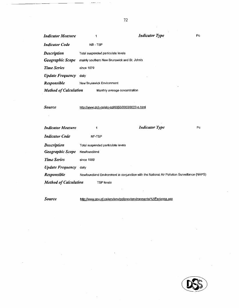
72
Indicator Type Indicator Measure 1
Indicator Code NB - TSP
Description Total suspended particulate levels
Geographic Scope mainly soulhem New Brunswick and St. John’s
Time Series since 1979
Update Frequency daily
Responsible New Brunswick Environment
Method of Calculation Monthly average concentration
PC
Source http://www.qnb.calelq-e41/0355/0003/0023-e.htmi
Indicator Measure 1 Indicator Type PC
Indicator Code NF-TSP
Description Total suspended patiiculale level?.
Geographic $cope Newfoundland
Tinte Series sine 1999
Update Frequency daily
Responsible Newfoundland Environment in conjunction with the National Air Pollution Surveillance (NAPS)
Method of Calculalion TSP levels
Source
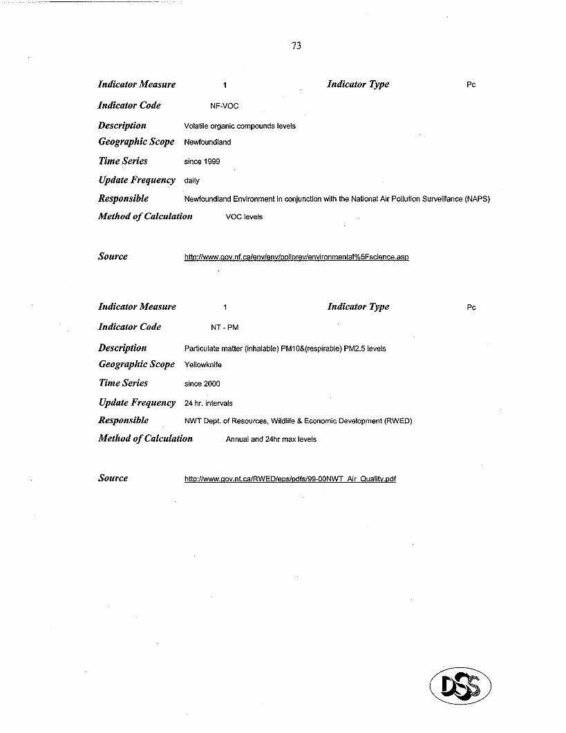
73
Indîcator Measure 1 Indicator Type PC
Indicator Code NF-VX
Description Volatile organic compounds levels
Geographic Scope Newioundland
Time Series since 1999
Update Frequency daily
Responsible Newfoundtand Environ!nent in conjunction wilh the National Air Pollution Surveillance (NAPS)
Mothod of Calculation voc le”els
Source htto:/lwww.~ov.nf.~ea/env/envl~ollprev/environmental%5Fscien~.asp
Indieator Measure 1 Indicator Type
Indicator Code NT-PM
Description Particulate matter (inhalable) PMlO&(respirable) PM2.5 levels
Geographic Scope Yetlowl<nife
Time Series since 2000
Update Frequency 24 hr. intervals
Responsible NWT Dept. of Reso~rcx?~. Witdtife 8 Economie Devetopment (RWED)
Method of Calculation Annual and 24hr max levels
source hU~://www.aov.nt.ca/RWE~/eps/pdfs/99.00NWT Air Qualitv.Ddf
PC
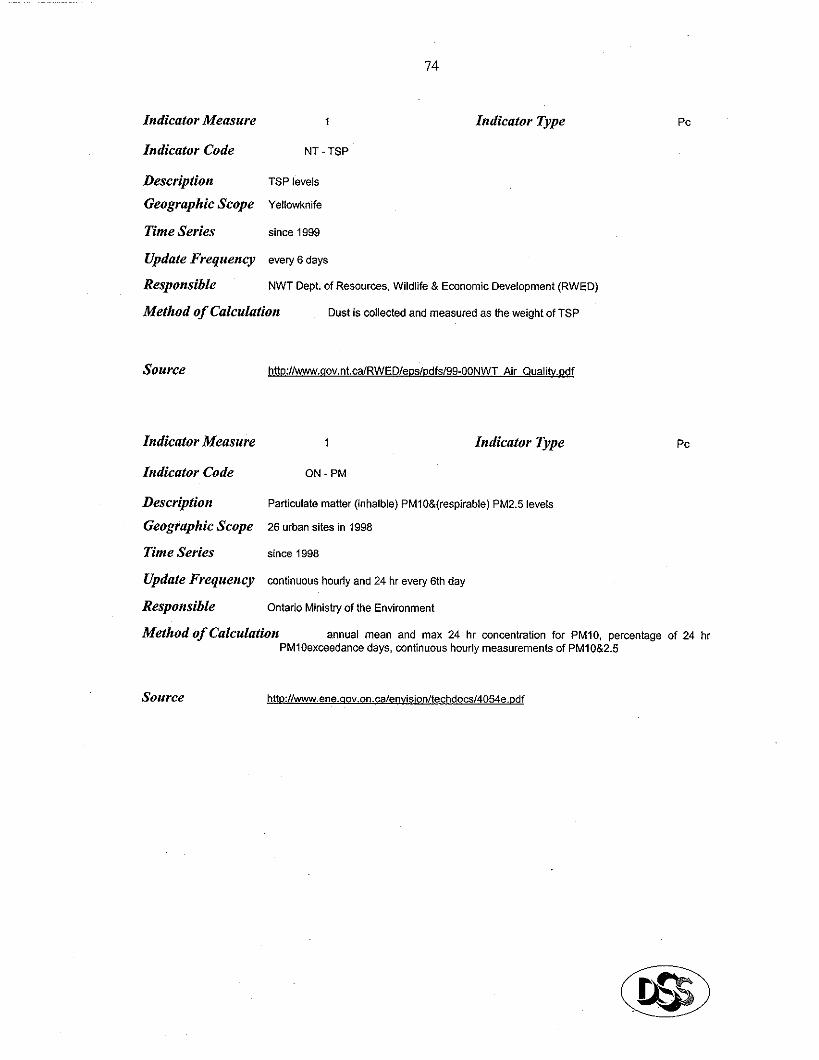
74
Indicator Measure 1 Indicator Type
Indicator Code NT TSP
Description TSP Ievels
Geographic Scope Yellowknife
Time Series sine 1999
Update Frequency eve~ 6 days
Responsible NWT Dept. of Resources. Wildlife & Ewnomic Development (RWED)
Metbod of Calculation DUS~ is cokcted and measured as the weighl of TSP
Source http://w.aov.nt.ca/RWED/eps/pdfs/99-OONWT Air Quality.pdf
PC
PC Indicator Measure 1 Indicator Type
Indicator Code QN-PM
Description Particulate matter (inhalble) PMlO&(respirable) PM2.5 levels
Geographic Ecope 26 urban sites in 1998
Time Series since 1998
Update Frequency wntinuous hourly and 24 hr every 6th day
Responsible Ontario Ministry of the Environment
Method of Calculation annual mean and max 24 hr concentration for PM10. percentage of 24 hr PMlOexceedance days, continuous hourly measurements of PM10&2.5
source
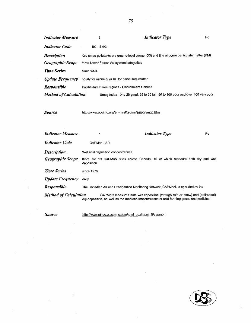
75
Indicator Measure 1 Indicator Type PC
Indicator Code SC - SMG
Description Key smog pollutank are ground-level ozone (03) and fine airbome particulate matter (PM)
Geographic Scope three Louer Fraser Valley moniloring sites
Time Series ?.ince 1994
Update Frequency hourly for ozone & 24 hr. for particulate matter
Responsible Pacifie and Yukon regions - Environment Canada
Method of Calci&tion Smog index - 0 to 25 good. 25 to 50 fair, 50 to 100 poor and over 100 very poor
Source http://www.ecoinfo.ora~env ind/reaionl~moa/smo~.htm
Indicator Measure 1 Indicator Type
Indicator Code CAPMon -AR
PC
Description Wet acid deposition concentrations
Geographicscope there are 19 CAPMoN sites across Canada, 10 of which measure both dry and wet deposition.
Tinte Series sine 1978
Update Frequency daily
Responsible The Canadian Air and Precipitation Monitoring Network, CAPMoN. is operated by the
Method of Calculation CAPMoN measures bath wet deposition (through min or snow) and (estimated) dry deposition, as well as the ambient concentrations of acid forming gases and particles.
Source
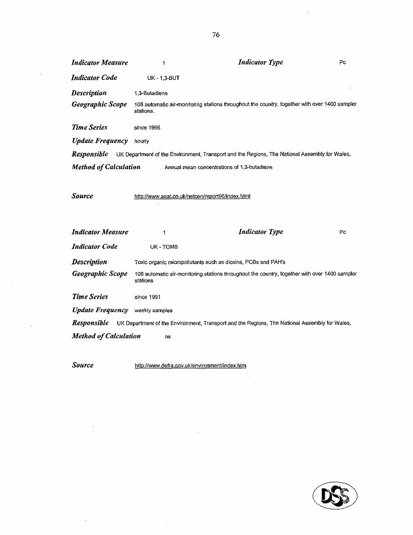
76
Indicator Ma~sure 1 Indicator Type PC
Indicator Code UK . 1,3-BUT
D<scription 1.3~Butadiene
Geographic Scope 108 automatic air-monitoring stations throughout the country. together with over 1400 sampler stations.
Tinte Series since 1996
Update Frequency houdy
Responsible UK Department of the Environment. Transport and the Regions. The National Assembly for Wales,
Method of Calculalion Annuat mean cowentraticns of 1 ,bbutadiene
Source hnp://www.aeat.co.uklnetcenlreportg6lindex.html
Indicator Measure 1 Indicator Type PC
Indicator Code UK-TOMB
Description Toxic organic micropollutants such as dioxins, PCBs and PA&
Geographic Scope 108 automatic air-monitoring stations throughout the country. togetherwith over 1400 sampler stations
Time Series since 1991
Vpdate Frequency weekly samples
Responsible UK Cepaiment of the Environment. Transport and the Regions. The National Assembly for Wales.
Method of Calculation ns
Source http://www.defra.qov.uklenvironmentlindex.htm
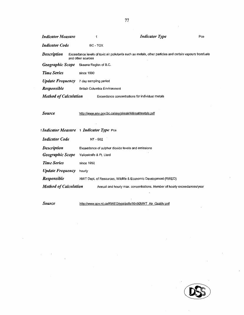
Indicator Measure 1 Indicator Type PCl?
Indicator Code SC - TOX
Description Exceedance levels of toxic air pollutants such as met&, other particles and certain vapeurs iranfuels and other sources
Geographic Scope Skeena Region of S.C.
Tinte Series since 1990
Update Frequency 7 day sampling period
Responsible Sritish Columbia Environment
Method of Calculation Exceedance concentrations for individual metals
Source
f Indicator Measure 1 Indicator Type PC~
Indicator Code NT - SO2
Description Exceedance of sulphur dioxide levels and emissions
Geographic Scope Yellowknife & Ft. Liard
Tinte Series *ince 1992
Update Frequency hourly
Responsible NWT Dept. of Resources, Wildlife B Economie Development (RWED)
Method of Calculation Annual and hourly max. concentrations. Number of houdy exceedanceslyear
source httr>://w.w.qov.nt.ca/RWED/eQs/Qdfs/99-OONWT Air QualitV.Qdf
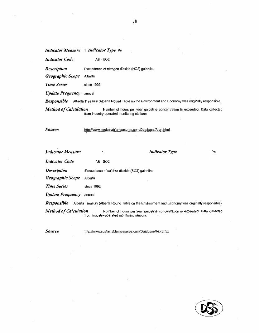
78
Indicator Measure 1 Indicator Type le
Indicator Code A0 - NO2
Description Exceedance of nitrogen dioxide (N02) guideline
Geographic Scope Alberta
Time Series sine 1992
Update Frequency annual
Responsible Alberta Treaswy (Alberta Round Table on the Environment and Economywas originally responsible)
Method of Calculation Number of heurs per year guideline concentration is exceeded. Data collected from indus@-operated monitoring stations
Source httQ://www.sustainablemeasures.com/Database/Alb~.html
Pe Indicator Measure 1 Indicator Type
Indicator Code AS - SO2
Description Exceedance of sulphur dioxide (SOZ) guideline
Geographic Scope Alberta
Time Series since 1992
Update Frequency muai
Responsible Alberta Treasuv (Alberta Round Table on the Environment and Economy was originally responsible)
Method of Calculation Number of hours per year guideline concentration is exceeded. Data collected from industry-operated monitoring stations
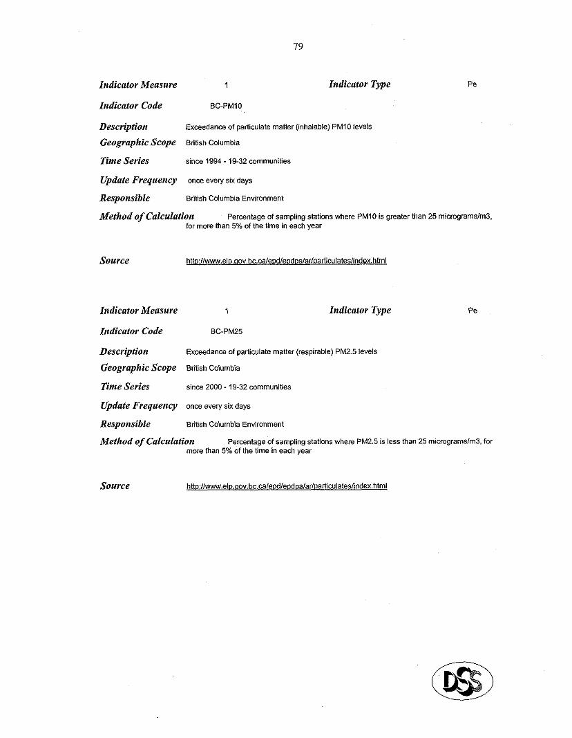
79
Indicator Measure 1
Indicator Code EC-PM10
Indicator Type
Description Exceedance of particulate matter (inhalable) PM10 levels
Geographic Scope British Columbia
Time Series since 1994 - 19-32 communities
Update Frequency once evet~ six days
Responsible British Columbia Environment
Method of Calculation Percentage of sampling stations where PM10 is greater than 25 microgramslm3. for more than 5% of the lime in each year
Source
Indicator Measure 1 Indicator Type Pe
Indicator Code W-PM25
Description Exceedance of patiiculate matter (respirable) PM2.5 levels
Geographic Scope British Columbia
Time Series since 2000 - 19-32 communities
Update Frequency once ewy six days
Responsible British Columbia Environment
Method of Calculation Percentage of sampling stations where PM2.5 is less than 25 microgramslm3. for more lhan 5% of the time in each yeat
Source
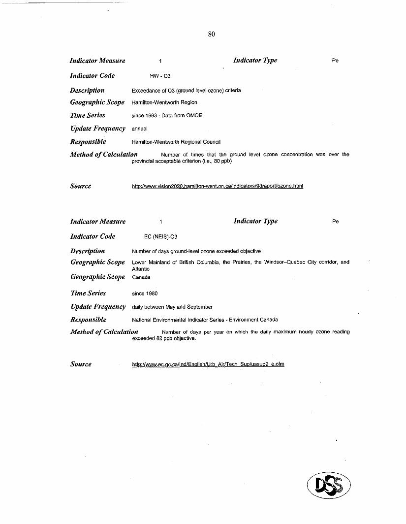
80
Indicator Measùre 1
Indicator Code WI-03
Indicator Type Pe
Description Exceedance of 03 (ground kvel ozone) criteria
Geographic Scope Hamilton-Wenlworlh Region
Tinte Series since 1993 -Data from OMOE
Update Frequency annual
Responsible Hamilton-Wentwotih Regional Council
Method of Calculalion Number of times that the ground level ozone concentration was over the provincial acceptable criterion (i.e., SO ppb)
SOWC.9 http://www.vision202O.hamilton-went.on.calindicatoB/98report/ozone.html
Indicator Measure 1 Indicator Type Pe
Indicator Code EC (NEIS)-03
Description Number of days gmund-level ozone exceeded objective
Geographic SCOpe Laver Mainland of British Columbia, the Prairies, the Windsor-Quebec City corddor, and Atlantic
Geographic Scope Canada
Time Series since 1980
@date Frequency daily between May and September
Responsible National Environmental Indicator Series - Environ!nent Canada
Method of Calculalion Number of days per year on which the daily maximum hourly ozone radin9 exceeded 82 ppb objective.
Source h~p:llwww.ec.ac.callndlEnalish/Vrb AirITech Su~luasup2 e.cfm
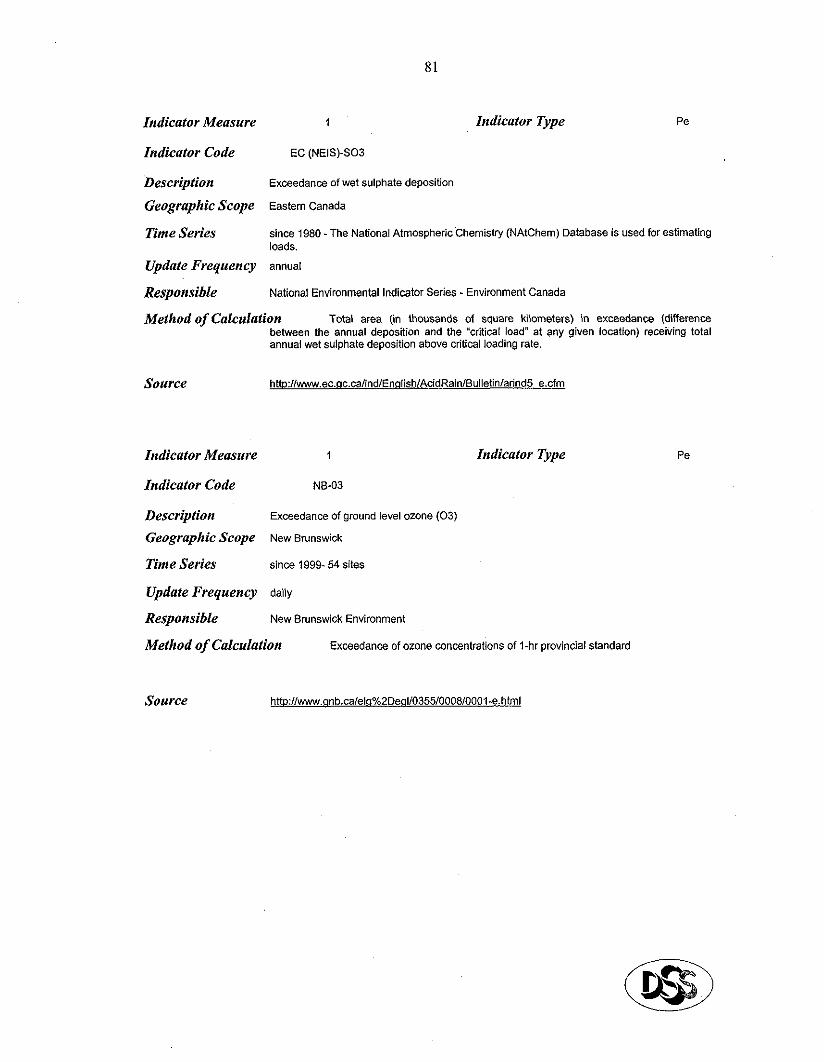
81
Indicator Measure
Indicator Code
Bescription
GeogYaphic Scope
Tinte Series
Update Frequency
Responsible
Indicator Type Pe 1
EC (NEWSOB
Exceedance of wet sulphate deposition
Eastem Canada
sine 1980 - The National Atmospheric Chemistry (NAtChem) Database is used for estimating loads.
annlIaI
National Environmental Indicator Series - Environment Canada
Method of Calculaiion Total area (in thousands of square kilometers) in exceedance (difference betwen the annual deposition and the “critical load” at any given location) receiving total annual wet sulphate deposition above critical loading rate.
Source http:/lwww.ec.~c.ca/ind/En4lishlAcidRainlBulletinladnd5 e.cfm
Indicator Measure
Indicator Code
1
NB-03
Indicator Type
Description Exceedance of gmund level ozone (03)
Geographic Scope New Brunswick
Time Series since 1999.54 sites
Update Frequency daily
Responsible New Brunswick Environment
Method of Calculation Exceedance of ozone concentrations of l-hr provincial standard
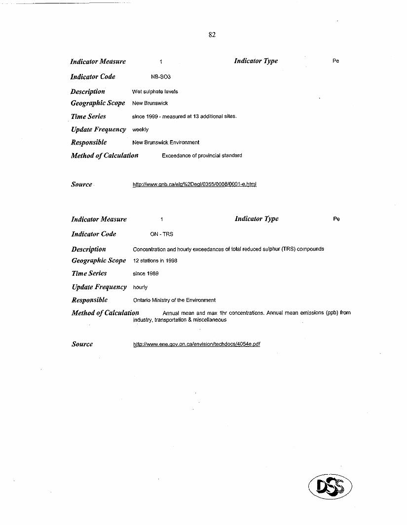
82
Indicator Type Indicator Measure 1
Indicutor Code NS-SO3
Description wet sulphate lewls
Geographic Scope New Brunswick
Time Series since 1999 - measured at 13 additional sites.
Update Frequency weehly
Responsible New Brunswick Environment
Pe
Method of Calculation Exceedance of provincial standard
Source httD://www.unb.ca/elq%2De91/0355/0008/0001-e.html
Indicator Measure 1 Indicator Type Pe
Indicator Code ON - TRS
Description Concentration and houdy exceedances of total reduced sulphur (TRS) COmQoUnds
Geographic Scope 12 stations in 1998
Tinte Series since 1989
Update Frequency hourly
Responsible Ontario Ministry of the Environment
Method of Calculation An~al mean and max Ihr concentrations. Annual mean emissions (Qpb) from industv. transportation & miscelaneous
Source
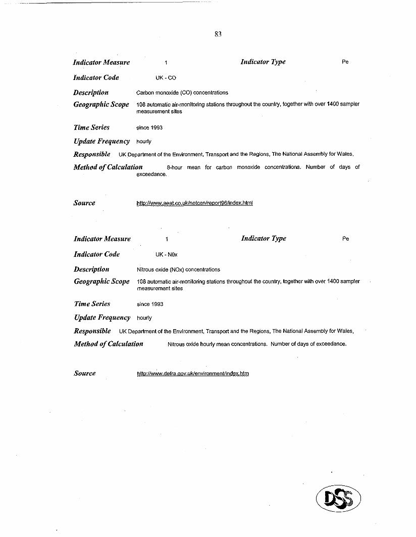
83
Indicator M&~~ure 1 Indicator Type Pe
Indicator Code UK-CO
Description Carbon monoxide (CO) concentrations
Geographic Scope 108 automatic air-monitoring stations throughout the country. together with over 1400 sampler measurement sites
Tinte Series sine 1993
Update Frequency hourly
Responsible UK Department of the Environment, Transport and the Regions, The National Assembly for Wates,
Method of Calculation S-hou mean for carbon monoxide concentrations. Number of days of exceedance.
Source hnp:llwww.aeat.w.uk<Inetcen/repo~96lindex.html
Indicator Measure 1 Indicator Type Pe
Indicator Code UK - NOx
Description Nitrous aide (NOx) concentrations
Geographic Scope 108 automatic air-monitoring stations throughout the wuntry, together with over 1400 sampler measurement sites
Time Series since 1993
Update Frequency hourly
Responsible UK Department of the Environment, Transport and the Regions, The National Assemply for Wales,
Method of Caiculation Nitrous oxide hourly mean concentrations. Number of days of exceedance.
Source http://www.defra.qov.uWenvironmenVindex.htm
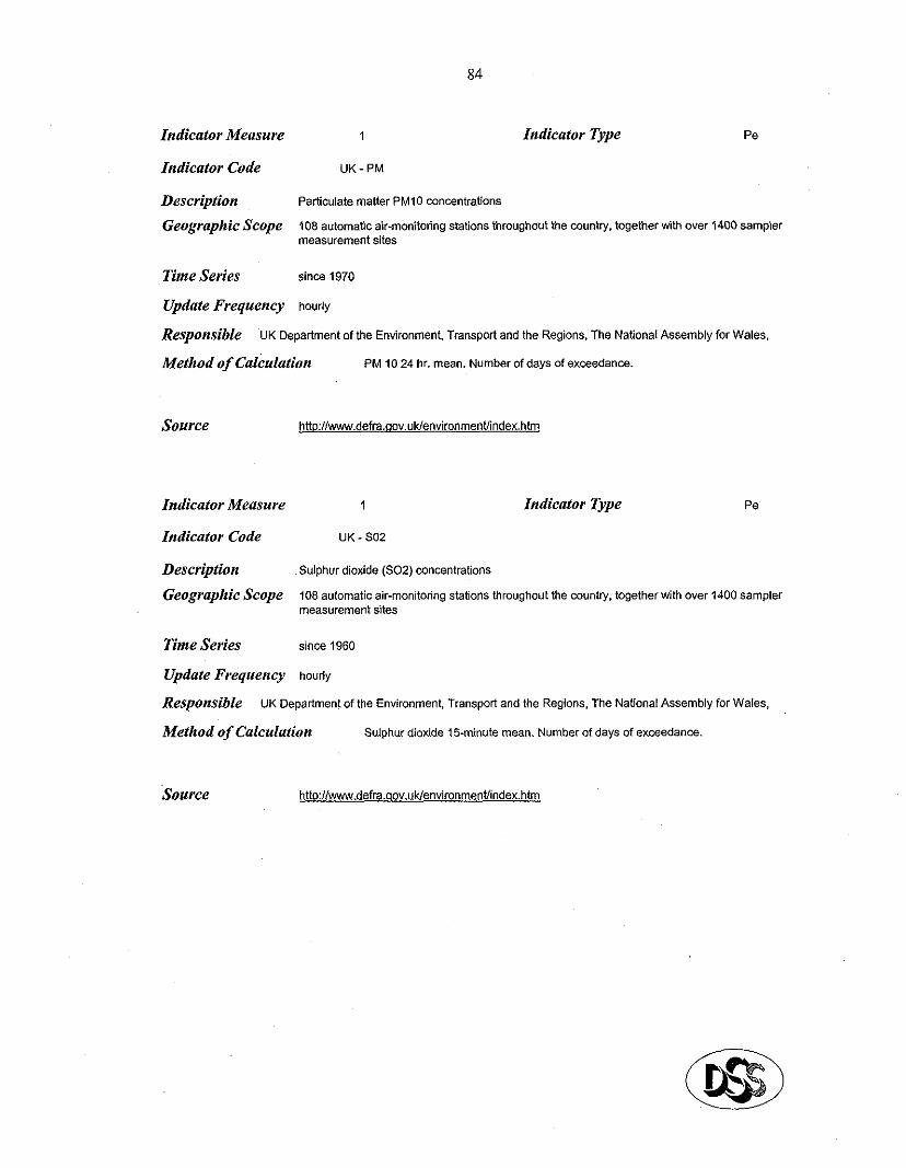
Indicator Memure 1
Indicator Code UK-PM
84
Indicator Type Pe
Description Partialaie matter PM10 concentrations
Geographic Scope 108 automatic air-monitoring stations throughout the country. together with ovet 1400 sampler masurement sites
Time Series since 1970
Update Frequency nour~y
Responsible UK Department of the Environment, Transport and tha Regions. The National Assembly for Wales.
Method of Calculation PM 10 24 hr. mean. Number of days ofexceedance.
Source htto://www.defra.qav.uldenvironmentlindex.htm
Indicator Measure 1 Indicator Type Pe
Indicator Code UK - SO2
Description Sulphur dioxide (502) concentrations
Geographic SCOpe 108 automatic air-monitoring stations throughout the counby. together with ow 1400 sampler measurement sites
Tinte Series since 1960
Update Frequency hourly
Responsible UK Department of the Environment, Transport and the Regions. The National Assembly for Wales,
Method of Calculation SuIphu dioxide 15minute mean. Number ai days of exceedance.
Source htto:llwww.defra.aov.uk/environment/index.htm
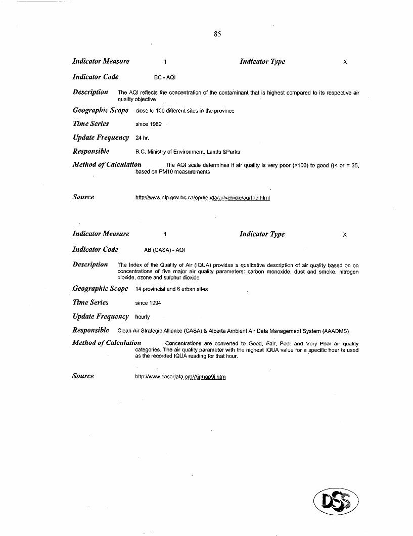
85
Indicator Measure 1 Indicator Type X
Indicator Code SC - AQI
Description The AQI reflects the concentration of the contaminant that is highest compared to its respective air quality objective
Geographic Scope close to 100 different sites in lhe province
Tinte Series sine 1989
Update Frequency 24 hr.
Responsible EX. Minis@ of Environment, La?ds &Parks
Method of Calculation The AQI scale determines if air quality is very poor (>iOO) to good ((< or = 36. based on PM10 measuremenis
Source htlD!//www.el~.qov.bc.~lePdlepdalarlvehiclelaq~c.hlml
Indicator Measure 1 Indicator Type X
Indicator Code AS (CASA) - AQI
Description The Index of the Quality of Air (IQUA) provides a qualitative descdption of air quality based on on concentrations of We major air quality parameters: carbon monoxide, dust and smoke, nitrogen dioxide. ozone and sulphur dioxide
Geographic Scope 14 provincial and 6 urban sites
Tinte Series sine3 1994
Update Frequency hourly
Responsible Clean Air Strategic Alliance (CASA) & Alberta Ambient Air Data Management System (AAADMS)
Method of Calculaiion Concentrations are convetied to Good. Fair. Poor and Very Pour air quality categories. The air quality parameter with the highest IQUA value for a ~pecific heur is used as the recaded IQUA reading for lhal heur.
Source httt):llwww.casadata.ora/AinapSi.htm
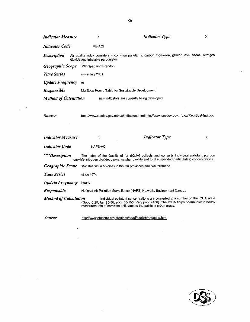
86
Indicator Measure 1 Indicator Type x
Indicator Code MB-AQI
Description Air qualily index considers 4 common pollutants: carbon monoxide. ground level ozone. nitrogen dioxide and inhalable patticulates.
Geographic Scope Winnipeg and Srandon
Time Series since .Ju,y 2001
Update Frequency ns
Responsible Manitoba Round Table for Sustainable Developmeni
Method of Calculation ns - Indicators are currently being developed
Source
Indicator Measure 1 Indicator Type X
Indicator Code NAPS-AQI
****Description The Index of the Quality of Air (IQUA) colle& and con~eTts individual pdlutant (carbon monoxide. nitrogen dioxide, ozone. sulphur dioxide and total suspended particulaies) concentrations
Geographic Scope 152 stations in 55 cities in the ten provinces and bvo territories
Time Series since 1974
Update Frequency hourly
Responsible National Air Pollution Surveillance (NAPS) Nebwrk, Environ!nent Canada
Method of Calculation IndividuaI poIlutant concentrations are converted to a number on the IQUA sale (Good 0.25. fair 25.50. poor 50.100. Vay poor MOO). The IQUA helps wmmunicate houdy measurements of common pollutants to the public in urban areas.
Source http:/l~.etcentre.orqldivisions/aaad/ e.html
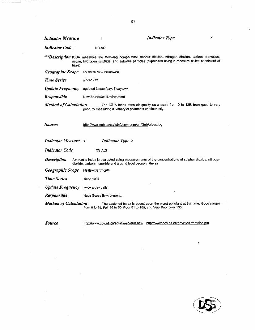
87
Indicator Measure 1 Indicator Type X
Indicator Code NS-MI
***Description QUA measures the following compouods: sulphur dioxide. nitrogen dioxide. carbon monoxide. ozone. hydrogen sulphide. and ah-borne partides (expressed using a masure called coefF&nt Of haze)
Geographic Scope southem New Brunswick
Time Series since1979
Update Frequency updated Btimes/day, 7 dayslwk
Responsible New Brunswick Environment
Method of Calculation The ICXJA index rates air quality on a scale from 0 to 125, from good ta very poor. by measuring a variety of pollutants continuously.
Source httr>:llwww.~nb.calscno$2/environm/airlGetValues.idc
Indicator Measure 1 Indicator Type x
Indicator Code NS-AIX
Description Air quality index is evaluated using measurements of the concentrations of sulphur dioxide. nitrogen dioxide, carbon monoxide and ground level ozone in the air
Geographic Scope Halifax-Dartmouth
Tinte Series since 1997
Update Frequency twice a day daily
Responsible Nova Scotia Environment.
Method of Calculation The assigned index is based upon the worst poIlutant at the tirne. Good ranges from 0 to 25. Fair 26 to 50. Poor 51 to 100, an* Very Poor over 100
Source
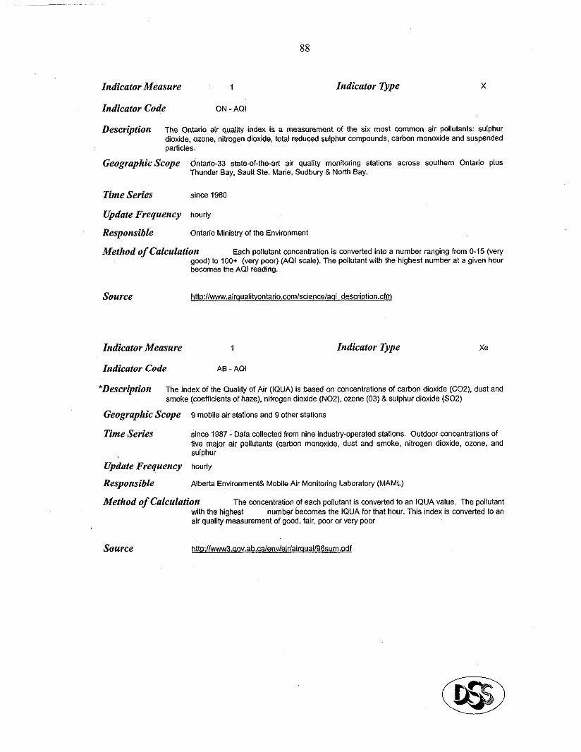
88
Indicator Measure 1 Indicator Type X
Indicator CO& ON - AQI
Description The Ontado air quality index is a measurement of the six mas1 common air Qohtants: sulphur dioxide. ozone. nitrogen dioxide. total reduced su!Qhur compounds, carbon monoxide and suspended pZtiCk?S.
Geographic Scope Ontario-33 state-of-the-art air quality monitoring stations across southem Ontario plus Thunder Bay. Sault Ste. Marie. Sudbury & North Bay.
Tinte Series since 1960
Update Frequency hourly
Responsible Ontario Ministry of the Environment
Method of Calculation Each pollutant concentration is cwwerted into a number ranging from Q-15 (very go@ to tOg+ (very poor) (AQI scale). The Qollutant with the highest number at a given heur becornes the AQI reading.
Source htt~://www.airqualitontario.com/sciencelaqi descriptiorxcfm
Indicator Measure
Indicator Code
1
AS - AQI
Indicator Type X‘2
*Description The Index of the Quality of Air (IQUA) is based on concentrations of ca-bon dioxide (COZ). dust and smoke (coefficients of haze). nitrogen dioxide (NOZ). ozone (03) & sulphut dioxide (SOZ)
Geographic Scope
Time Series
Update Frequency Responsible
9 mobile air stations and 9 other stations
since 1967 -Data collected from nine industiy-operated stations. Outdoor concentrations of five maior air poUutants (carbon monoxtde. dust and smoke. nitrogen dioxide, ozone, and sulphur
hourly
Alberta Environment& Mobile Air Monitoring Laboratow (MAML)
Method of Calculation The concentration of each pollutant is converted to an IQUA value. The pollutant ~4th the highest number becomes the IQUA for that hou. This index is converted to an air quality measurement of gond, fair. poor or very poor
Source
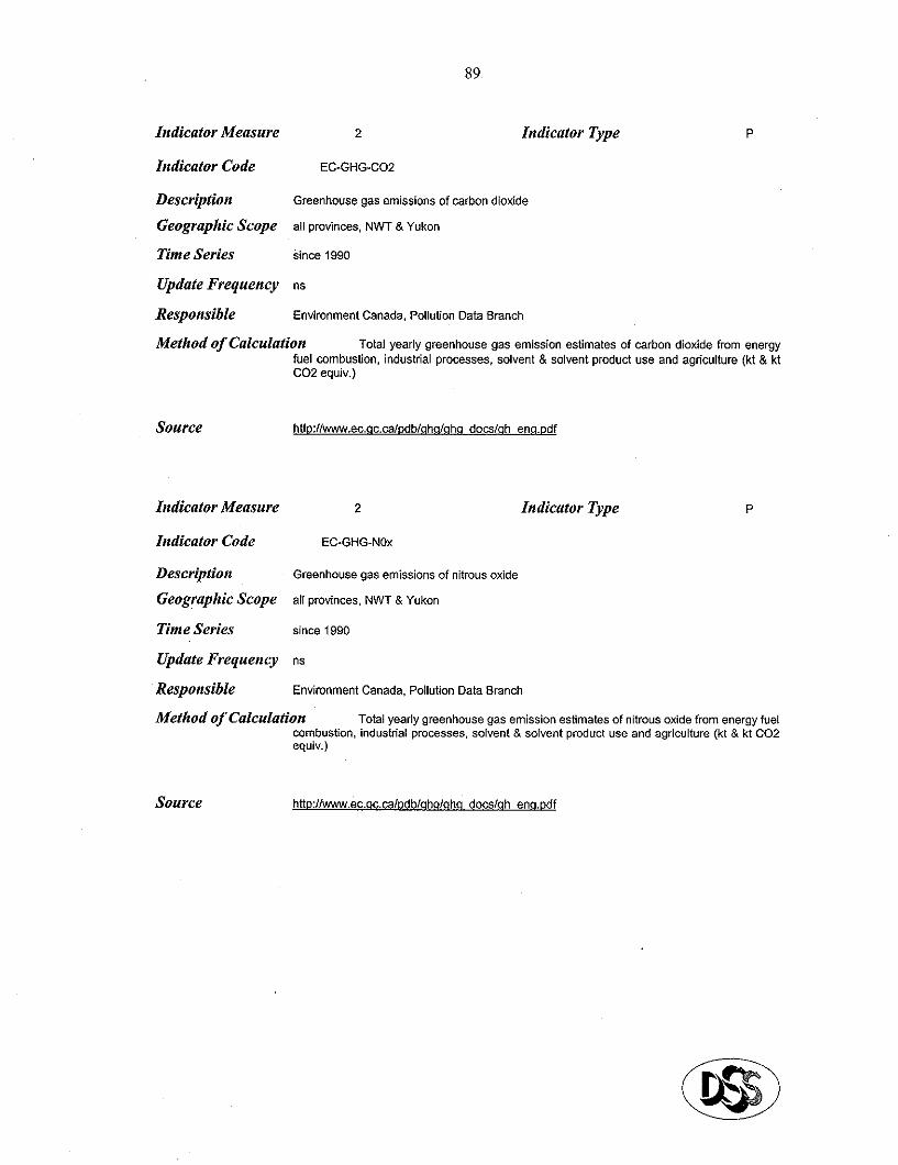
89
Indicator Measure 2 Indicator Type
Indicator Code EC-GHG-CO2
P
Description Greenhouse gas emissions of carbon dioxide
Geographic Scope a11 provinces. NWT 8. ~ul<on
Time Series S!llce 1990
Update Frequency ns
Responsible Environment Canada, Pollution Data Bmnch
Method of Calculaiion Total yearly greenhouse gas emission estimates of carbon dioxide from energy fuel combustion, industdal processes. solvent & solvent product use and agrkzulture (kt & kt CO2 equiv.)
Source http://www.ec.ac.ca/db/qhq/qhq docs,qh enq.,,df
Indicator Measure
Indicator Code
Description Geographic Scope
Tinte Series
Update Frequency
Responsible
2 Zndicator Type
EC-GHG-NOx
Greenhouse gas emissions of nitrous oxide
all provinces, NWT & Yukon
since 1990
“S
Environment Canada, Pollution Data Branch
P
Method of Calculation Total yearly greenhouse gas emission estimates of nitrous aide irom energy fuel combustion, industriaI processes, soIvent 8 solvent product use and agriculture (kt & kt CO2 equiv.)
Source hnp:llwww.ec.qc.calpdblahqlqhq docslqh enq.Ddf

90
Indicator Measure 2 Indicator Type P
Indicator Code EC-GHG-SF6
Description Greenhouse gas emissions sulphur hexafluoride
Geographic Scope all provinces. NWT & Yukon
Time Series since 1990
Update Frequency ns
Responsible Environment Canada. Pollution data Branch
Method of Calculation Total yearly greenhouse gas em,issions estimaies of sulphur hexailuoride from energy fuel combustion, industrial processes. solvent & solvent product use and agriculture (kt & kt CO2 equiv.)
Indicator Measure
lndicator Code
Description Geographie Scope
Time Series
Update Frequency
Responsible
hnp:llwww.ec.ac.calpdblqhqlqha docslah enapdf
2
EC-GHG-CH4
Indicator Type P
Greenhouse 9% emissions of methane
all provinces, NWT & Yukon
since 1990
“S
Environment Canada. Pollution data Branch. Greenhouse Gas Div.
Method of Calculation Total yeady greenhouse 9% emission estimates of methane from energy fuel combustion, industria! processes. solvent & solvent prduct use and agriculture (kt & kt CO2 equiv.)
Source http:liwww.ec.qc.ca/pdb/qhq/qhq docslah enq.pdf
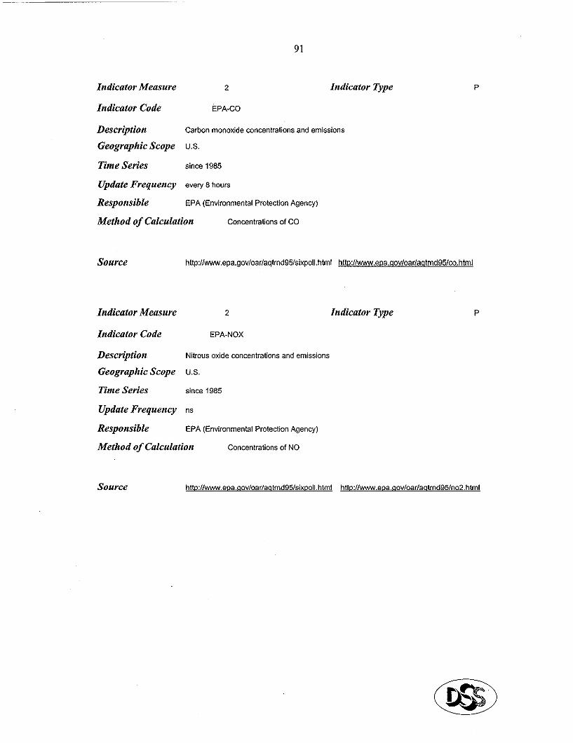
91
Indicator Measure 2 Indicator Type
Indicator Code EPA-CO
Description Carbon monoxide concentrations and emissions
Geographic Scope US.
Time Series since 1985
Update Frequency every 8 heurs
Responsible EPA (Environmental Protection Agency)
Method of Calculation Concentralions of CO
P
Source http://www.epa.gov/oar/aqtrnd95/sixpoll.html http:/lwww.epa.qov/oarlaqtmd95l~.html
Indicator Measure 2 Indicator Type
Indicator Code EPA-NOX
Description Nitrous oxide concentrations and emissions
Geographic Scope us.
Tinte Series since 1985
Update Frequency ns
Responsible EPA (Environmental Protection Agency)
Method of Calculation Concentrations of NO
P
92
Indicafor Measure 2 Indicator Type
Indicator Code EPA-03
Description Ground level ozone concentralions and emissions
Geographic Scope U.S.
Time Series since 1985
Update Frequency hourly
Responsible EPA (Environmental Protection Agency)
Method of Calculation concentmoons of ground bml ozone
P
Source hlt~:Il~.e~a.~oVarla~trnd95lsixL)OIl.html http:l/www.e~a.~ov/oarla~trnd9Slo3.html
Iadicator Measure 2 Indicafor Type P
Indicator Code EPA-Pb
Description Lead cxmcentrations and emissions Geographic Scope US.
Time Series since 1985
Update Frequency ns
Responsible EPA (Environmental Protection Agency)
Method of Calculation Concentrations of lead
93
Indicator Measure 2 Indicator Type
Indicator Code EPA-SO2
Description Sulphur dioxide concentrations and emissions
Geographic Ecope NS.
Time Series since 1985
Update Frequency daily
Responsible EPA (Environmental Protection Agency)
Method of Calculation Concentrations of SO2
P
Indicator Measure 2 Indicator Type
Indicator Code ME-SO2
Description Sutphur dioxide (SOZ) emissions
Geographic Ecope Vin Fton and Thompson
Tinte Series since July 2001
Update Frequency ns
Responsible Manitoba Round Table for Sustainable Development
Method of Calculation ns - tndicators are currently being developed
P
Source htto://www.susdev.~ov.mb.ca/Rep-Sust-lnd.dac
94
Indicator Type Indicator Measure 2 P
Indicator Code EC (NEAS)-CO2
Description Carbon dioxide emissions and GDP
Geographic Scope canada
Time Series since 1958
Update Frequency quatier~y
Responsible National Environmental tndicator Series - Environ!nent Canada
Method of Calculation Carbon dioxide emissions from fossil fuels and Grass DomesBc Product (GDP) are esiimated based on energy consumption data from Statislics Canada Catalogues
Source htlp:/l~.ec.ac.ca/IndlEn~lish/Climate~ech Su~lccsu~Ol e.cfm
Indicator Measure 2 Indicator Type P
Indicator Code EC (NEIS)-GHC
Description Global atmospheric concentrations of greenhouse gases (carbon dioxide)
Geographic Scope global -Hawaii and NWT
Tinte Series since 1959
Update Frequency hourly
Responsible National Environmental Indicator series - Environment Canada
Method of Calculation Annual atmospheric concentrations
Source httD://www.ec.ac.M/Ind/English/Climate~ech Su1)/ccsu[105 e.cfm
95
Zndicator Measure 2 Zndicator Type
Zndicator Code EC (NEIS)-GHM
Description Global atmospheric u>ncentratiOns of greenhouse gases (methane)
Geographic Scope global - 28 land-based sites plus ships
Time Series sine 1984
Update Frequency weekly
Responsible National Environmental Indicator Series - Environment Canada
Method of Calculation Average global atmospheric concentrations
Source http:l/www.ec.ac.~IIndlEnq~ishlClimate~ech SuplccsupO8 e.cfm
Indicator Measure 2 Zndicator Type
P
P
Zndicator Code EC (NEIS) GHN
Description Global atmospheric concentrations of greenhouse gases (nitrous oxide)
Geographic Scope global - 7 stations
Time Series sine 1977
Update Frequency 24 measurements per day are taken at each site.
Responsible National Environmental Indicator Series Environment Canada
Method of Calculation Average global atmospheric concentrations
Source http:/lw.ec.wxa/Ind/Enalish/ClimatelTech SuplccsupO9 e.cfm
96
Indicator Measure 2 Indicator Type P
Indicator Code EC (NEIS)-NOX
Description Emissions of nitrogen aides
Geographic Scope ~astern Canada
Time Series since 1980
Update Frequency annual
Responsible National Environmentil Indicator Sedes - Environment Canada
Method of Calculation Total wmbined emissions from mobile sources (69.. cars. trucks. rail, air. and marine transportation) and stationary sources) reported fmm all monitored point sources plus a,lowa”ce for non-monitored sources.
Source http:liwww.ec.ac.ca/indlEn~lishlAcidRainlSulletin~arind2 e.Cfm
Indicator Measure 2 Indicator Type P
Indicator Code EC (NUS)-SO2
Description Emissions of sulphur dioxide
Geographic Scope ~astern Canada
Time Seriez sine 1.980
Update Frequency annual
Responsible National Environmental Indicator Series - Environment Canada
Method of Calculation Total combined emissions ((in million tonnes) from smelting of metzIl Ores, p0wer genemtion and other sources) from all monitored point sources plus allowance for non- monitored sources.
Source htt~:/lwww.ec.ac.ca/ind/Enalish/AcidRainlSu~~etinlarindl e.Cfm
97
Indicator Measure 2 Indicator Type P
Indicator Code ,ON - NO2
Description Nitrogen oxide (NO2) concentration levels and emissions
Geographic Scope 27 sites
Tinte Series sine 1989
Update Frequency hourly
Responsible Ontario Ministry of the Environment
Method of Calculation Annual mean and 24 hr max concentration. Annual emissions (ppb) from industry and transporiation
Source hno:llwww.ene.~~v.on.calenvisionltechdo~l4O~e.~f
Indicator Measure
Indicator Code
2
ON - SO2
Indicator Type P
Description Sulphur dioxide (SO2) concentration levels and emissions
Geographic Scope 27 sites in 1998
Tinte Series sine 1971
Update Frequency hourly
Responsible Ontario Ministry of the Environment
Method of Calculation Annual mean and 24 hr max conwntration. Annual emissions (ppb) irom industw and transportation
Source
98
Indicator Measure 2 Indicator Type
Indicator Code ON- CO
P
Descripfion Carbon monoxide (CO) concentration tevels and emissioos
Geographic Scope 21 sites
Tinte Series sine 1989
Vpdate Frequency hourly
Responsible Ontario Ministry of the Environment
Method of Calculation I hr and 8 hr maximum concentrations. Annuat emissions (kilotonnes) ïrom industry, transportation
Source http:llwww.ene.~ov.on.calenvision/techdo~l4054e.Ddf
Indicator Measure 2 Indicator Type
Indicator Code Pc)-03
Description Ground tevel ozone (03) emissions
Geographic Ecope Quebec - 13 st@ons
Tirne Series sine 1975
Vpdate Frequency hourly
Responsible Qu6bec Enuironnement
Method of Calculation Hourly ozone concentrations and 1 hr. exceedances
P
Source
99
Indicator Measure 2 Indicator Type P
Indicator Code PQ-CO
Description Carbon monoxide emissions
Geographic Scope Quebec- 7 stations
Time Series since 1975
Update Frequency 1 hr & 8 hr.
Responsible Québec Environnement
Method of Calculation Annual emissons of ca-bon monoxide lrom fuel combustion, industrial & residential and mean annual concentrations
Source http:II~.menv.gouv.~c.ca/airl~ualite-enli~dex.htm
Indicator Measure
Indicator Code
2
PQ - H2S
Indicator Type P
Description Hydrogen sulphide (H2S) emissions
Geographic Scope Quebec
Tinte Series Since 1979
Update Frequency ns
Responsible QuBbec Environnement
Method of Calculation Annual mean and 1 hr. exceedances (as a percentage) of hydrogen sulphide concentrations
Source
100
Indicator Meusure 2 Indicatov Type P
Indicator Code PQ - NOx
Description Nitrous oxide (NOx) emissions
Geographic Scope Quebec
Time Series since 1975
Update Frequency 1 hr.. 8 hr. & 24 hr.
Responsible Québec Environnement
Method of Calculatfon Annual emissions of nitrogen dioxide irom transportation 8 industv. Mean annual concentrations of N02. Exceedances of 1 hr., 8 hr & 24 hr. NO2 concentrations.
Source http:II~.menv.aouv.ac.~lairlaualite-en~ndex.hlm
Indicator Measure
Indiizator Code
Description
Geographic Scope
Time Series
Update Frequency
Responsible
2
PQ - SO2
Indicator Type
Sulphur dioxide S02) emissions
Quebec
since 1975
ns
Qu&bec Environnement
P
Method of Calculation Annual emissions of sulphur dioxide from combustion, transportation & incineration. Exceedances of 1 hr and 24 hr. SO2 levels
Source
101
Indicator Me~sure 2 Indicator Type PC
Indicator Code AB GHG
Description Greenhouse gas emissions
Geographic Scope Alberta
Tinte Series sine 1990
Update Frequency annual
Responsible Alberta Treasury (Alberta Round Table on the Environment and Econamy was odginally responsible.
Method of Calculation Greenhouse gas emissions of carbon dioxide (CD2). ozone, methane, nitrous oxide. and hydrofluorocarbons
Source htto://www.sustainablemeasures.com/Datab.html
Indicator Measure 2 Indicator Type PC
Indicator Code BC-GHG
Description Total greenhouse gas emissions inctuding carbon dioxide. methane, nitrous aide, ozone, HF&.
Geographic Scope Eiittsh Columbia
Tinte Series since 1970
Update Frequency ns
Responsible British Columbia Environment
Method of Calculation Total output of dl greenhouse gas emissions measured in megatonnes of CO2 equivalents
Source
102
Indicator Measure 2 Indicator Type
Indicator Code EC-GHG-HFC
PC
Description Greenhouse gas emissions of HF&
Geographic Scope a11 provinces, NWT & Yukon
Tinte Series since 1990
Update Frequency ns
Responsible Environment Canada, Pollution Data Branch
hfethod of Calculation Total yearly greenhouse 9% emission estimaies of HFCs from energy fuel combustion, industdal processes. solvent & solvent product use and agriculture (kt 8. Id CO2 equiv.)
Source htt~:/l~.ec.ac.ca/db/qhalqhq docslah enq.pdf
Indicator Measure 2 Indicator Type
Indicator Code EC-GHG-PFC
PC
Description Greenhouse gas emissions of PFc’s
Geographic Scope au provinces. NWT & Yukon
Tinte Series since 1990
Update Freqaency ns
Responsible Environment Canada, Pollution Data Eranch
Method of Calculation Total yearly greenhouse gas emission estimates of PFCs from energy fuel combustion. indusirial processes. solvent 8 solvent product use and agriculture (kt 8 Id CO2 equiv.)
Source hUr>:l~.ec.qc.calDdb/qhqlahq dow,qh e”q.Ddf
103
Indicator Measure 2 Indicator Type
Indicator Code EPA-PM
Description Partiwlate matter PM10 concentrations and emissions
Geographic Scope US.
Time Series since 1985
Update Frequency daily
Responsible EPA (Environmental Protection Agency)
Method of Calculation Concentrations of PM10
PC
Source httD://www.epa.aov/oar/aatrnd95/sixooll.ht~, http:l/www.e~a.aovloarlautrnd95l~mlO.html
Indicator Measure 2
Indicator Code GPI - GHG
Description Greenhouse gas emissions
Geographic Scope ‘Nova Scotia
Time Series na
Update Frequency ns
Responsible GPI Atlantic
Method of Calculation ns
hdicator Type PG
Source
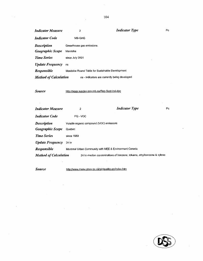
104
Indicator Measure 2
Indicator Code MB-GHG
Indicator Type PC
Description Greenhouse gas emissions.
Geographic Scope Manitoba
Tinte Series since July 2001
Update Frequency ns
Responsible Manitoba Round Table for Sustainable Development
Method of Calculation ns _ Indicators are cwently being developed
Source hlt~:IIWWW.susdev.qov.mb.ca/Rel)-Sust-lnd.doc
PC Zndicator Measure 2 Indicator Type
Indicator Code Pc) - voc
Description Volatile organic compound n/OC) emissions
Geographic Scope Quebec
Tinte Series since 1989
Update Frequency 24 hr
Responsible Montreal Urban Community tith M!E & Environment Canada
Method of Calculation 24 hr media concentrations of benzene, toluene, ethylbenzene & xykne
Source
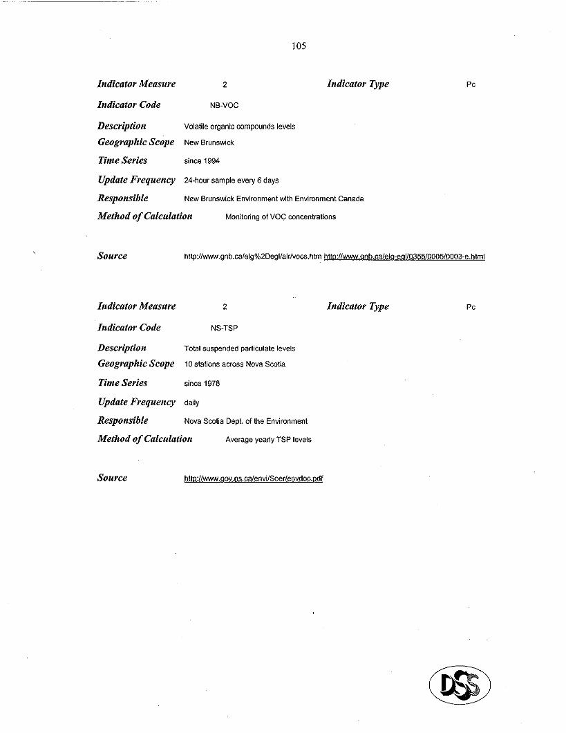
105
Indicator Type Indicator M?asure 2
Indicator Code NB-VOC
Description Volatile organic wmpounds levels
Geographic Scope New Brunswick
Tinte Series since 1994
Update Frequency 24.heur sampk? every 6 days
Responsible New Brunswick Environment with Environment Canada
Method of Calculation Monitoring of VOC concentrations
PC
Source http://www.gnb.calelg%2Degl/aidvocs.htm http://~.~nb.ca/e14-e4110355/00051000l
Indicator Measure 2 Indicator Type PC
Indicator Code NS-TSP
Description Total suspended QatiCUlate levels
Geographic Scope 10 stations across Nova Scotia
Tinte Series since 1976
Update Frequency daily
Responsible Nom Scotia Dept. of the Environment
Method of Calculation Average yearly TSP levels
Source http:/lwww.aov.ns.calenvilSoer/envdoc.odf
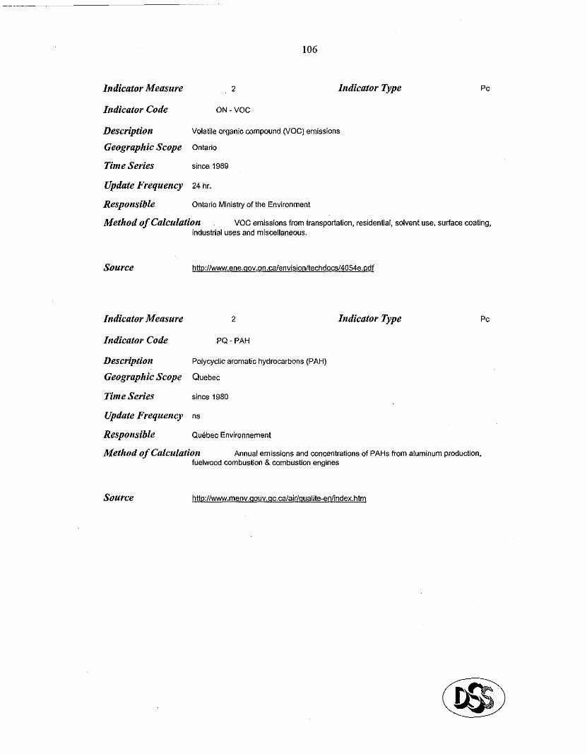
106
Indicator Measure 2 Indicator Type PC
Indicator Code ON - VOC
Description Volatile organic compound (VOC) emissions
Geographic Scope Ontario
Time Series since 1989
Update Frequency 24 hr.
Responsible Ontario Ministry of the Environment
Method of Calculation VOC emissions lrom transportation. residential. solvent use. surface cnating, industrial uses and misc&aneous.
Source htt~://www.ene.~ov.on.ca/envision/techdo~l4054e.Qdf
PC Indicator Measure 2 Indicator Type
Indicator Code Pc) PAH
Description Polycycllc aromatic hydrocarbons (PAH)
Geographîc Scope Quebec
Time Series since 1980
Update Frequency ns
Responsible Québec Environnement
Method of Calculation Annual emissions and concentrations of PAHs from aluminum production, fuelwood combustion 8 combustion engines
Source
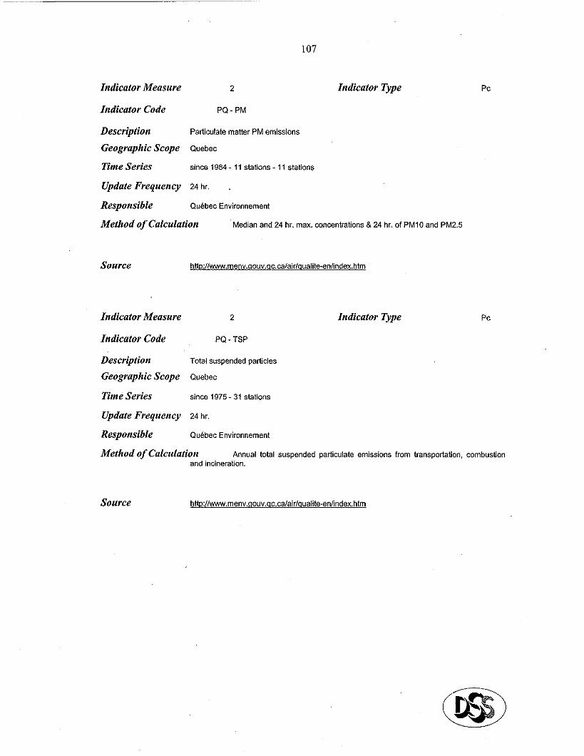
107
Indicaior Measure 2
Indicator Code PC)-PM
Indicator Type
Description Particulate matter PM emissions
Geographic Scope Quebec
Time Series since 1984 11 stations - 11 stations
Update Frequency 24 hr. .
Responsible Québec Environnement
Method of Calculation Median and 24 hr. max. concentrations & 24 hr. of PM10 and PM2.5
Indicator Measure 2
Indicator Code PQ - TSP
Description Total suspended padides
Geographic Scope Quebec
Time Series since 1975 31 stations
Update Frequency 24 hr.
Responsible Qu&bec Environnement
Indicator Type
PC
PC
Method of Calculation Annual total suspended parkulate emissions from transportation. combustion and incineration.
Source h~o:l/www.menv.aouv.~c.ca/airlaualite-enlindex.htm
Indîcator Measure 2
Indicator Code NT-GHG
108
Zndicator Type PCe
Description Greenhouse 9as emissions
Geographic Scope Northwesl Territories
Time Series sine 1990
Update Frequency ns
Responsible NWT Dept. of Resources. Wildlife & Economie Development (RWED)
Method of Calculation Greenhouse 9% emissions
Source
Indicator Measure 2 Indicator Type
Indicator Code NT-CO2
Description Carbon dioxide emissions
Geographic Scope Northwest Territories
Time Series since 1990
Update Frequency ns
Responsible NWT De@. of Resources, Wildlife & Economie Development (RWED)
Method of Calculaiion Carbon dioxide emissions
Source
Pe
109
Indicator Measure
Indicator Code
Description Geographic Scope
Time Series
Update Frequency
Responsible
3
EC (NEIS)-03D
Indicator Type PC
New supplies of ozone-depleting substances
Canada
since 1979
an!lual
National Environmental Indicator Series - Environment Canada
Method of Calculation Estimates (kilotonnes expressed as WC-11 equivalents) of the folloting ozone- depleting substances produced, imported, and expotted annually; chlorofluorocxbons bromochlorofiuoroca~ons. hydïochlorofluorocarbons. methyl bromide. Grass Domestic Product (GDP)
Source
Indicator Measure 3 Indicator Type
Indicator Code EC-NEIS-OJDG
Pc
Description Global atmospheric concentrations of ozone-depleting substances
Geographic Scope global
Time Series since 1977 eight stations covering a latitudinal range from 83% to 90”s currently provide data
Update Frequency ns
Responsible National Environmental Indicator Series - Environment Canada
Method of Calculation Concentration of WC-11 and CFC-12 (ppt) in the lower atmosphere: eight stations covering a latitudinal range from 83”N to 90’s currently provide data
~OUrCehttp:II~.ec.~c.wlind/EnalishlO~one~ech SuplstsuDB e.cfm
110
Indicator Measure 3 Indicator Type
Indicator Code EC (NEIS)-03DG
Description New supplies of ozone-depleting substances
Geographic Scope global
Time Series since 1950
Update Frequency annua~
Responsible National Environmental fndicator Series - Environment Canada
PC
Method of Calculation Annuaf estimates of CFCs (kifotonnes) wmprised of CFCs and Grass Wodd Product (GWP).
Source http:/l~.ec.~c.calInd/EnqlishlO~o~e~ech Sup/stsup2 e.cfm
111
Indicator Type
Indicator Code EPA-UV
Description Ultraviolet radiation kvels
Geographic Scope U.S.
Time Series sine 1997
Update Frequency unknown
Responsible EPA (Environmental Protection Agency)
Method of Calculaiion Measurement of UV-net
Source htl~:llwww.e[>a.qovluv-net/
Indicator Measure 4 Indicator Type I
Indicator Code HW-HD
Description Hospital discharges for respiratory illnesses
Geographic Scope Hamilton-Wentwotih Region
Time Series since 1993
Update Frequency ‘annual
Responsible Hamilton-Wentworlh Regional Council
Method of Cakulation Annual rate of hospital admissionsldischarges for respimtay illness per 100.000 peop~e.
Source
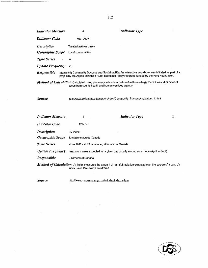
112
Indicator Measure 4
Indicator Code MG - ASM
Indicator Type I
Description Treated asthma cases
Geographic Scope LO~~I communities
Time Series ns
Update Frequency ns
Responsible Measuring Community Success and Sustainability: An Interactive Workbook was initiated as part of a project by the Aspen Institut& Rural Economie Policy Program. funded by the Ford Foundation.
Method of C&&tiOn Calculated using Qharmacy sales data (sales of asthmalallergy medicine) and number of cases fmm county health and human sewices agency.
Source htt~:ll~.a~.iaState.edu/centerslrdevlCommunitv Success/indicator4-l.html
Indicator Measure 4 Indicator Type X
Indicator Code EC-UV
Description UV index.
Geographic Scope 13 stations across Canada
Time Series sine 1992 - at 13 monitodng sites âcms~ Canada.
Update Frequency maximum value expected for a given day usually around solar noon (AQril to Sept).
Responsible Environment Canada
Method Of CUhhtiOn UV index measures the amount of harmful radiation expected over the course of a day. UV index Q-4 is low. over 9 is extreme
Source httQ:llwww.msc-smc.ec.qc.ca/uvindex/index e.htm