air quality and early-life mortality

Air Quality and Early-Life MortalityEvidence from Indonesia’s Wildfires

Seema Jayachandran

a b s t r a c t

Smoke from massive wildfires blanketed Indonesia in late 1997. This paperexamines the impact that this air pollution (particulate matter) had on fetal,infant, and child mortality. Exploiting the sharp timing and spatial patternsof the pollution and inferring deaths from ‘‘missing children’’ in the 2000Indonesian Census, I find that the pollution led to 15,600 missing children inIndonesia (1.2 percent of the affected birth cohorts). Prenatal exposure topollution drives the result. The effect size is much larger in poorer areas,suggesting that differential effects of pollution contribute to thesocioeconomic gradient in health.

I. Introduction

Between August and November 1997, forest fires engulfed largeparts of Indonesia, destroying over 12 million acres. Most of the fires were startedintentionally by logging companies and palm oil producers clearing land to plantnew crop.1 Because of the dry, windy conditions caused by El Nino, the fires burnedout of control and spread rapidly. In November, rains finally doused the fires.

Seema Jayachandran is an assistant professor of economics at Stanford University and a facultyresearch fellow at the National Bureau of Economic Research. She is grateful to Doug Almond, JanetCurrie, Erica Field, Dan Kammen, Michael Kremer, Doug McKee, Ben Olken, Sarah Reber, DuncanThomas, seminar participants at AEA, Berkeley, BREAD, Columbia, Maryland, Stanford GSB, UCLA,and Harvard/MIT/BU, and three anonymous referees for helpful comments. She also thanks Kok-HoeChan and Daniel Chen for data and Nadeem Karmali and Rika Christanto for excellent researchassistance. The data used in this article are available for purchase through the Indonesian StatisticsBureau (Badan Pusat Statistik). The author will assist other scholars who have purchased the data toreproduce the data set used here. Contact [email protected].½Submitted December 2006; accepted May 2008�ISSN 022-166X E-ISSN 1548-8004 � 2009 by the Board of Regents of the University of Wisconsin System

THE JOURNAL OF HUMAN RESOURCES d 44 d 4

1. The Indonesian Minister of Forestry estimated that ‘‘½commercial� plantations caused some 80 percent ofthe forest fires,’’ and that small farmers caused the remainder (Straits Times, September 3, 1997). Rabindran(2001), using satellite data on land use, finds that the 1997 incidence of fires on plantations was higher thanthe ‘‘natural’’ level (based on a benchmark from conservation areas), but the incidence of fires on smallfarms was at its natural level.

While the fires were burning, much of Indonesia, especially Sumatra and Kalimantanwhere the fires were concentrated, was blanketed in smoke. This paper examines fetal,infant, and child mortality caused by the episode of poor air quality (specifically,high levels of particulate matter). Daily satellite measurements of airborne smokeat locations across Indonesia provide information on the spatial and temporalpatterns of the pollution. The outcome is fetal, infant, and child mortality before agethree—hereafter called early-life mortality—and is inferred from ‘‘missing children’’in the 2000 Census, overcoming the lack of mortality records for Indonesia and thesmall samples in surveys with mortality data.

The paper finds that higher levels of pollution caused a substantial decline in thesize of the surviving cohort, and that exposure to pollution during the last trimesterin utero is the most damaging. The fire-induced increase in air pollution is associ-ated with a 1.2 percent decrease in cohort size. This estimate is the average acrossIndonesia for the five birth-month cohorts with high third-trimester exposureto pollution; it implies that 15,600 child, infant and fetal deaths are attributableto the pollution. Indonesia’s under-three mortality rate during this period was about6 percent; if the estimate is driven mainly by child and infant deaths (rather thanfetal deaths), this represents a 20 percent increase in under-three mortality.

The paper also finds a striking difference in the mortality effects of pollutionbetween richer and poorer places. Pollution has twice the effect in districts with be-low-median consumption compared to districts with above-median consumption.Individuals in poorer areas could be more susceptible to pollution because of lowerbaseline health, more limited options for avoiding the pollution, or less access tomedical care. Another possibility is that people exposed to indoor air pollution ona daily basis suffered more acute health effects from the wildfires because they re-ceived a double dose of pollution. Consistent with this view, the effects are largerin areas where more people cook with wood-burning stoves. Surprisingly, mother’seducation does not seem to play a role. While these correlations do not pin downcausal relationships, they provide suggestive evidence on why the poor are especiallyvulnerable to the health effects of pollution and add to our understanding of the so-cioeconomic (SES) gradient in health (Marmot et al. 1991; Smith 1999). An openquestion in the literature is how much of the health gradient is due to low-SES indi-viduals being more likely to suffer adverse health shocks and how much is due to agiven health shock having worse consequences for the poor (Case, Lubotsky, andPaxson 2002; Currie and. Hyson 1999). This paper provides some evidence for thesecond mechanism: People faced a common environmental-cum-health shock, andthe consequences were much worse for the poor.

This study examines an extreme episode of increased pollution, which has advan-tages for empirical identification. The abruptness and magnitude of the pollution areuseful for identifying when in early life exposure to pollution is most harmful. Inutero exposure is found to be especially important, suggesting that targeting pregnantwomen should be a priority of public health efforts concerning air pollution. Theextreme level of pollution, however, also means that one must be cautious about ex-trapolating the effect size to more typical levels of pollution.

That being said, rampant wildfires are not uncommon in Indonesia and other coun-tries, mainly in Southeast Asia and Latin America, where fire is used to clear land.Most cost estimates of the 1997 Indonesian fires have focused on destroyed timber,

Jayachandran 917

reduced worker productivity, and lost tourism and are in the range of $2 to 3 billion(Tacconi 2003). This study shows that the health costs of the fires are much larger:Assuming a value of a statistical life of $1 million, the early-life mortality costs alonewere over $15 billion.2 The costs of the fires very likely overwhelm the benefits tofirms from setting them; the annual revenue from Indonesia’s timber and palm oilindustries at this time was less than $7 billion.

The remainder of the paper is organized as follows. Section II provides back-ground on the link between pollution and health and on the Indonesian fires. SectionIII describes the data and empirical strategy. Section IV presents the results, andSection V concludes.

II. Background

A. Link between air pollution and early-life mortality

1. Related Literature

Previous related work includes that by Chay and Greenstone (2003b), who usevariation across the United States in how much the 1980–81 recession lowered pol-lution and find that better air quality reduced infant mortality. Chay and Greenstone(2003a) also find that pollution abatement after the Clean Air Act of 1970 led to adecline in infant deaths.3 Currie and Neidell (2005), in their study of California inthe 1990s, find that exposure to carbon monoxide and other air pollutants during themonth of birth is associated with infant mortality.4

In addition, there have been studies on the adult health effects of Indonesia’s 1997fires. Emmanuel (2000) finds no increase in mortality but an increase in respiratory-related hospitalizations in nearby Singapore. Sastry (2002) finds increased mortalityfor older adults on the day after a high-pollution day in Malaysia. Frankenberg,Thomas, and McKee (2004) compare adult health outcomes in 1993 and 1997for areas in Indonesia with high versus low exposure to the 1997 smoke. Theyfind that pollution reduced people’s ability to perform strenuous tasks and othermeasures of health. Their data set covers 321 of the 4,000 subdistricts in Indonesia,and only one of Kalimantan’s four provinces is in their sample. Thus, one advantageof this paper is its broader geographic coverage, which allows one to explore hetero-geneous effects and nonlinearities in the health impact of pollution, for example.

2. This value of a statistical life (VLS) is calculated using $5 million in 1996 dollars as the value for theUnited States from Viscusi and Aldy (2003), Murphy and Topel (2006), and the U.S. Environmental Pro-tection Agency (2000); an income elasticity of a VSL of 0.6 from Viscusi and Aldy (2003); and the fact thatIndonesia’s per capita gross domestic product was one tenth of U.S. GDP. Note that the total health costsfrom early-life exposure to the pollution would also include costs among those who survived. Recent worksuggests that there could be long-term consequences among surviving fetuses (Barker 1990; Almond 2006).3. Other natural experiments used to measure health effects of air pollution include the temporary closureof a steel mill in Utah during a labor dispute; the reduction in traffic during the 1996 Olympics in Atlanta;and involuntary relocation of military families (Pope, Schwartz, and Ransom 1992; Friedman et al. 2001;Lleras-Muney 2006).4. For research on pollution and infant mortality outside the United States, see, for example, Bobak andLeon (1992) on the Czech Republic, Loomis et al. (1999) on Mexico, and Her Majesty’s Public Health Ser-vice (1954) on the 1952 London ‘‘killer fog’’ episode.

918 The Journal of Human Resources

Another important advance over previous work is the use of both the sharp timingand extensive regional variation of the pollution; one can then identify causal effectswhile allowing for considerable unobserved heterogeneity across time and place.

2. Physiological Effects of Pollution

Smoke from burning wood and vegetation, or biomass smoke, consists of very fineparticles (organic compounds and elemental carbon) suspended in gas. Fine par-ticles less than 10 microns (mm) and especially less than 2.5 mm in diameter areconsidered the most harmful to health because they are small enough to be inhaledand transported deep into the lungs. For biomass smoke, the modal size of particlesis between 0.2 and 0.4 mm, and 80 to 95 percent of particles are smaller than 2.5 mm(Hueglin et al. 1997).

Prenatal and postnatal exposure to air pollution could affect fetal or infant healththrough several pathways. Postnatal exposure can contribute to acute respiratory in-fection, a leading cause of infant death. Prenatal exposure can affect fetal develop-ment, first, because pollution inhaled by the mother interferes with her health,which in turn disrupts fetal nutrition and oxygen flow, and, second, because toxicantscross the placenta. Several studies find a link between air pollution and fetal growthretardation or shorter gestation period, both of which are associated with low birth-weight (Dejmek et al. 1999; Wang et al. 1997; Berkowitz et al. 2003). The biologicalmechanisms behind these pregnancy outcomes are related to the main toxicant inparticulate matter, polycyclic aromatic hydrocarbons (PAHs). In utero exposure toparticulate matter has been associated with a greater prevalence of PAH-DNAadducts on the placenta, and PAH-DNA adducts, in turn, are correlated with low birthweight, small head circumference, preterm delivery, and fetal deaths (Perera et al.1998; Hatch, Warburton, and Santella 1990). Laboratory experiments on rats haveconfirmed most of these effects (Rigdon and Rennels 1964; MacKenzie and Ange-vine 1981). PAHs disrupt central nervous system activity of the fetus, and during crit-ical growth periods such as the third trimester, the disruption has a pronounced effecton fetal growth. PAHs are also hypothesized to reduce nutrient flow to the fetusby suppressing estrogenic and endocrine activity and by binding to placental growthfactor receptors (Perera et al. 1999).

B. Description of the Indonesian Fires

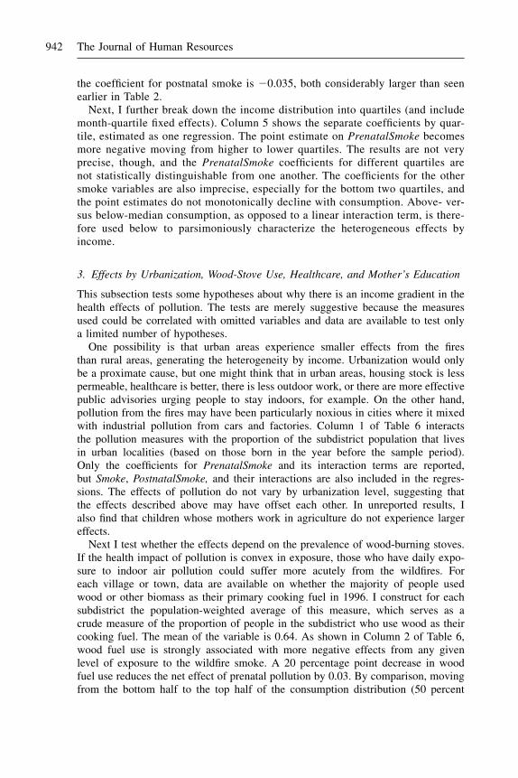
The 1997 dry season in Indonesia was particularly dry. Figure 1 shows the monthlyrainfall recorded at a meteorological station in South Sumatra in 1997 compared toprevious years. The 1997 dry season was both severe and prolonged: Rainfallamounts in June to September were lower than usual, and the rainy season wasdelayed until November. The rest of Indonesia experienced rainfall patterns similarto Sumatra’s.

Fires are commonly used in Indonesia to clear land for cultivation, and the dry sea-son is considered an opportune time to set fires because the vegetation burns quickly.Industrial farmers burn forest land in order to replant it with palm or timber trees, andsmall farmers use ‘‘slash–and–burn’’ techniques in which land is cleared with fire toready it for cultivation. In addition, logging companies are thought to have set some

Jayachandran 919

virgin forests on fire since the government would then designate the degraded land asavailable for logging.

With expansion of the timber and palm oil industries in Indonesia, many tracts offorest land have become commercially developed, and logged-over land is moreprone to fires than pristine forest.5 Roads running through forests act as conduitsfor fire to spread, and with the canopy gone, the ground cover becomes drier andmore combustible and wind speeds are higher. Also, because logging firms weretaxed on the volume of wood products that left the forest, they often left behindwaste wood, even though it had economic value as fertilizer or wood chips.The left-behind debris wood made the forest more susceptible to fast-spreading fires(Barber and Schweithhelm 2000).

In September 1997, because of the dry conditions, the fires spread out of control.The Indonesian government made some attempt to fight the fires, but the effortswere ineffective. The fires continued until the rains arrived in November. The fireswere concentrated in Sumatra and Kalimantan. About 12 million acres were burned,8 million acres in Kalimantan (12 percent of its land area) and four million in Suma-tra (4 percent of its area). The practice of clearing land with fire is used throughoutIndonesia, and El Nino affected all of Indonesia. What set Sumatra and Kalimantanapart is that Indonesia’s forests are mainly in these areas. The majority of crop plan-tations are located in Sumatra, and plantations are a fast-growing use of land in Kali-mantan. Timber operations are also primarily in these regions.

Figure 1Rainfall at Palembang Airport meteorological station, South Sumatra, 1990-97

5. In 1996 forest products accounted for 10 percent of Indonesia’s gross domestic product, and Indonesiasupplied about 30 percent of the world palm oil market (Ross 2001).


The location of the smoke generally tracked the location of the fires, thoughbecause of wind patterns, not entirely. Fires were concentrated on the southern partsof Sumatra and Kalimantan, and these two areas experienced the most pollution.On the other hand, the northern half of Sumatra was strongly affected by smokewhile Java was relatively unaffected, yet neither of these areas experienced fires,for example.

A common measure of particulate matter is PM10, the concentration of particlesless than ten mm in diameter. The U.S. Environmental Protection Agency has seta PM10 standard of 150 micrograms per cubic meter (mg/m3) as the 24-hour averagethat should not be exceeded in a location more than once a year. During the 1997fires, the pollution in the hardest hit areas surpassed 1000 mg/m3 on several daysand exceeded 150 mg/m3 for long periods (Ostermann and Brauer 2001; Heil andGoldammer 2001). The pollution levels caused by the wildfires are comparable tolevels caused by indoor use of wood-burning stoves. The daily average PM10 levelfrom wood-burning stoves, which varies depending on the dwelling and durationof use, ranges from 200 to 5000 mg/m3 (Ezzati and Kammen 2002).

III. Empirical Strategy and Data

A. Empirical Model and Outcome Variable

The goal of the empirical analysis is to measure the effect that air pollution fromthe wildfires had an on early-life mortality. Ideally, there would be data on all preg-nancies indicating which ended in fetal, infant, or child death, and the followingequation would be estimated:

Survivejt ¼ b1Smokejt + dt + aj + ejt:ð1Þ

The variable Survivejt is the probability that fetuses whose due date is month t andwhose mothers reside at the time of the fires in subdistrict j survive to a certain point,such as live birth, one year, etc. The prediction is that b1 is negative, or that exposureto smoke around the time of birth reduces the probability of survival.

In practice, mortality records are unavailable for Indonesia, and survey samplesare too small to examine the effects of month-to-month fluctuations in pollution.For example, the 2002 Demographic and Health Survey has on average one birthand 0.05 recorded child deaths per district-month for the affected cohorts.6 Therefore,the approach I take is to infer early-life mortality by measuring ‘‘missing children.’’The outcome measure is the cohort size for a subdistrict-month calculated from thecomplete 2000 Census of Population for Indonesia. The estimating equation is

ln ðCohortSizeÞjt¼b1Smokejt+b2PrenatalSmokejt + b3PostnatalSmokejt + dt + aj + ejt

ð2ÞThe dependent variable, ln(CohortSize)jt, is the natural logarithm of the number of

people born in month t who are alive and residing in subdistrict j at the time of the 2000

6. Appendix 1 verifies that population counts from the Census move one-for-one with births and deaths inthe Demographic and Health Survey sample.

Jayachandran 921

Census. Smokejt is the pollution level in the month of birth, and PrenatalSmokejt

and PostnatalSmokejt are the pollution level before and after the month of birth. Eachobservation is weighted by the subdistrict’s population (the number of people enumer-ated in the Census who were born in the two years prior to the sample period).

An advantage of the Census compared to a survey is that the data are for the entirepopulation. Also, the outcome variable measures fetal deaths in addition to infantand child deaths, albeit without distinguishing between the different outcomes; mostsurveys do not collect data on fetal deaths. Finally, population counts are often bettermeasured than infant and child mortality because of underreporting of deaths andrecall error on dates of deaths.

There are several potential concerns about inferring mortality from survivors,however. Since the data come from a cross-section of survivors in June 2000, theoutcome represents a different length of survival for individuals born at differenttimes, and the mean level of survival will differ by cohort, independent of the fires.For a cohort born in December 1997 around the time of the fires, the outcome is sur-vival until age two and a half, while for an older cohort born in December 1996,the outcome is survival until age three and a half, for example.7 The inclusion ofbirthyear-birthmonth (hereafter, month) fixed effects in the regression will controlfor any average differences in survival by cohort.

In using ln(CohortSize) as a proxy for the early-life mortality rate, an assumptionis that, conditional on subdistrict and month fixed effects, pollution is not correlatedwith ln(Births). This seems like a reasonable assumption. First, by using a shortpanel, subdistrict fixed effects absorb most variation in the number of women ofchildbearing age and other determinants of fertility. Month effects control for fertilitytrends and seasonality. Second, it seems unlikely that there were large fluctuations infertility that coincided with the air pollution both spatially and temporally. Evenarea-specific trends could not explain the patterns since the sample includes controlperiods both before and after the fires; any omitted fertility shift causing bias wouldhave to be a short-term downward or upward spike in particular regions. In addition,Section IVB provides empirical evidence that fertility is unlikely to be a confoundingfactor.

Another concern is that if pollution affects the duration of pregnancies, then miss-ing children might result from the shifting of births from certain months to othermonths. If exposure to smoke induces preterm labor, then one would expect to seean excess of births followed by a deficit of births. In Section IVB, I examine andam able to reject that the results are an artifact of changes in gestation period.

There are also potential empirical concerns not unique to using ln(CohortSize) asthe dependent variable. First, pollution might affect not only mortality but also fer-tility. This would influence the population counts for the later ‘‘control’’ cohorts andcould lead to sample selection problems even if mortality were directly measured.I therefore restrict the sample to births occurring no more than eight months afterthe outbreak of the fires, or cohorts who were conceived before the fires. Second,the empirical model assumes that exposure to pollution just before or after birthaffects mortality, an assumption motivated by previous findings. However, exposure

7. One advantage of observing survival more than two years after the due date is that for deaths that occuraround birth, the estimates are less likely to reflect simply short-term ‘‘harvesting.’’


to pollution earlier in a pregnancy or later after birth also could affect health. If thecontrol cohorts are in fact also treated, though less intensely, then the results wouldunderestimate the true effects.

A third important concern arises from the fact that individuals are identified bytheir subdistrict of residence in 2000 rather than the subdistrict where their motherresided during the end of her pregnancy or just after giving birth. If families livingin high-smoke areas with children born around the time of the fires were more likelyto leave the area (either during or after the fires), then the cohort size would besmaller in areas more affected by pollution. Fortunately, one can directly examinethis concern since the Census collects the district of birth and the district of residencein 1995. As discussed in Section IVB, the results are identical using birthplace,current location, or mother’s location in 1995.

Table 1 presents the descriptive statistics. The sample comprises monthly observa-tions between December 1996 and May 1998 (18 months) for 3,751 subdistricts(kecamatan). Of this starting sample size of 67,518 observations, 64 observationsare dropped because the cohort size for the subdistrict-month is 0.8 There are onaverage 96 surviving children per observation. The larger administrative units inIndonesia are districts (kabupaten), of which there are 324 in the sample, and prov-inces, of which there are 29.

B. Pollution Variable

The measure of air pollution is the aerosol index from the Earth Probe Total OzoneMapping Spectrometer (TOMS), a satellite-based monitoring instrument. The aero-sol index tracks the amount of airborne smoke and dust and is calculated from theoptical depth, or the amount of light that microscopic airborne particles absorb orreflect. The TOMS index has been found to quite closely track particulate levels mea-sured by ground-based pollution monitors (Hsu et al. 1999). Ground monitor data arenot available for Indonesia for this period. The aerosol index runs from 22 to 7, witha higher index indicating more smoke and dust.

The TOMS data contain daily aerosol measures (which are constructed fromobservations taken over three days) for points on a 1 degree latitude by 1.25 degreelongitude grid. Adjacent grid points are approximately 175 kilometers (km) apart.The probe began collecting data in mid-1996, and the data I use begin in September1996. For each subdistrict, I calculate an interpolated daily pollution measurethat combines data from all TOMS grid points within a 100-km radius of the geo-graphic center of the subdistrict, weighted by the inverse distance between the sub-district and the grid point. The number of TOMS grid points that fall within thecatchment area of a subdistrict ranges from one to six and is on average four. Themean distance between a subdistrict’s center and the nearest grid point is 50 km.

8. The Census covers 3,962 subdistricts that make up 336 districts. For subdistricts dropped from the sam-ple, either the latitude and longitude could not be determined or there were no enumerated children formore than 15 percent of the monthly observations due to missing data or very small subdistrict size. In ad-dition, I drop four districts that make up Madura since this area received a large influx of return migrants in1999 in response to ethnic violence against them in Kalimantan, and also Aceh province where separatistviolence is thought to have affected the quality of the Census enumeration. The results are robust to drop-ping Irian Jaya, another area where unrest could have affected data quality.

Jayachandran 923

Table 1Descriptive Statistics

Mean Std. Dev.

Cohort size variablesCohort size (for subdistrict-month) 95.6 89.7Ln(cohort size) 4.8 0.8

Pollution variablesSmoke (median daily value for month) 0.087 0.424Prenatal smoke (Smoket-1,2,3) 0.095 0.330Postnatal smoke (Smoket+1,2,3) 0.074 0.342Proportion of days with high smoke (aerosol index > 0.75) 0.047 0.154Average smoke (daily values averaged for the month) 0.120 0.445Mean of smoke for Aug-Oct 1996 0.048 0.069Mean of smoke for Aug-Oct 1997 0.578 0.791Mean of prenatal smoke for Sept 1996–Jan 1997 0.038 0.052Mean of prenatal smoke for Sept 1997–Jan 1998 0.341 0.522

Other variablesFires (any fires) 0.157 0.364Intense fires (number x duration of fires $ 10 fire-days) 0.026 0.157Rainfall for June to November 1997 relative to 1990–95 0.480 0.241Ln(median 1996 household food consumption) 10.52 0.26

75th percentile 10.7150th percentile 10.4925th percentile 10.33

Median HH food consumption in 1996 / Median HH foodconsumption in 1998

0.742 0.070

National consumer price index (for food) 1.131 0.202Urbanization 0.57 0.39Wood as primary cooking fuel 0.636 0.413Doctors per 1,000 people 0.161 0.241Maternity clinics per 1,000 people 0.031 0.050Educated mothers (completed junior high) 0.386 0.215

Note: The sample consists of 67,454 subdistrict-birthmonths from December 1996 to May 1998. Sampleaverages are weighted by population (the number of people enumerated in the Census born in the year be-fore the sample period), except for cohort size for which the unweighted mean is shown. Cohort size is thenumber of people enumerated in the 2000 Census who were born in a subdistrict in a given month. Smokeis the monthly median of the daily TOMS aerosol index which is interpolated from TOMS grid pointswithin 100 km of the subdistrict’s geographic center and weighted by the inverse distance between the gridpoint and subdistrict center. Prenatal and Postnatal Smoke are averages of Smoke for the three months be-fore and after the month of birth. Fire-days is calculated from European Space Agency hot spots within 50km of the subdistrict’s center. Rainfall is measured at the nearest grid point on a 0.5 degree latitude/longi-tude grid and is the mean of 1997 rain relative to 1990–95 for June to November. Urbanization is the sub-district’s percent of births in urban areas based on those born 1994–96 and uses an indicator in the Censusof whether the respondent’s locality is rural or urban. Educated mothers is the percent of infants whosemother has completed junior high and is based on matching infants to mothers in the Census. Median foodconsumption is a per capita measure for each district that uses data from the 1996 and 1999 SUSENAShousehold survey. Consumer price index is from the Indonesian central bank. Healthcare variables are cal-culated for each subdistrict using the 1996 PODES (survey of village facilities). PODES and SUSENASdata are available for 63,158 observations.


The monthly measure is calculated as the median of the daily values, and I also usethe mean of the daily values and the number of days that exceed a threshold value of0.75.

The data include more than 3,700 subdistricts, but only 226 unique pollution gridpoints used. Interpolation adds spatial variation at a finer grain, but uncorrected stan-dard errors would nevertheless overestimate how much independent variation thereis in the pollution measure. Moreover, the actual pollution level is spatially correlated.Therefore I allow for clustering of errors among observations within an island group bymonth. The sample has ten island groups (Sumatra, Java, Sulawesi, Kalimantan, Bali,West Nusa Tenggara, East Nusa Tenggara, Irian Jaya, Maluku, and North Maluku).9

The estimating Equation 2 includes pollution in the month of birth (Smokejt) aswell as lags of Smokejt which measure exposure to pollution in utero, and leads thatmeasure exposure after birth. Note that Smokejt measures both prenatal and postnatalexposure, with the balance depending on when in the calendar month an individual isborn (the Census did not collect the specific date of birth, only the month). Itbecomes difficult to separately identify each lag and lead with precision, so the mainspecification uses an average of the pollution level for the three months before thebirth month (PrenatalSmokejt) and after the birth month (PostnatalSmokejt). The pop-ulation-weighted mean values of Smoke, PrenatalSmoke, and PostnatalSmoke are0.09, 0.10, and 0.07, as shown in Table 1. On average, the pollution index exceeds0.75 on 5 percent of days.

During the months of the fires, August to October 1997, the mean aerosol indexfor Indonesia was 0.58. For the same months in 1996, the mean was 0.05. Similarly,the mean of PrenatalSmoke was 0.34 for the most affected cohorts (births in Septem-ber 1997 to January 1998) while during the same months a year earlier, the mean was0.04. These gaps are helpful when interpreting the regression coefficients and quan-tifying the impact of the fires.

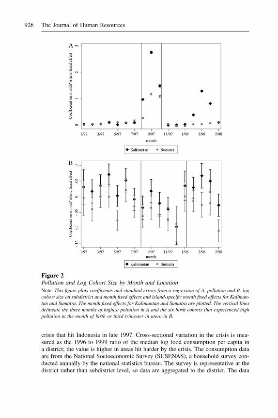
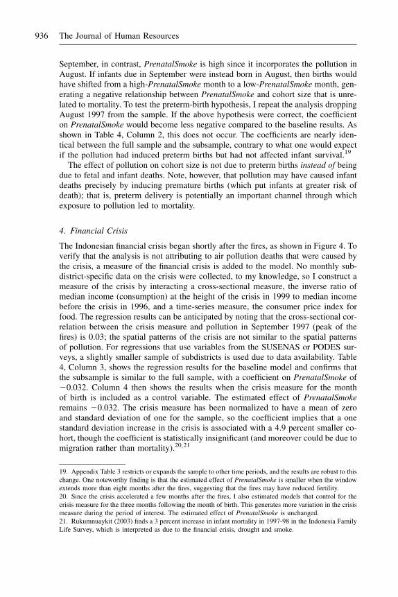
The intensity of smoke varied across Indonesia. Figure 2a shows the coefficients onisland-specific month fixed effects for Kalimantan and Sumatra, the hardest hit regions.The pollution was most severe during August to October 1997, both for Indonesia as awhole and in relative terms for Kalimantan and Sumatra, as shown. Kalimantan expe-rienced another episode of smoke in early 1998 after the rainy season ended.

Figure 2b plots the corresponding island-specific month effects using log cohortsize as the outcome variable. Intuitively, the identification strategy is to test whetherin the areas most affected by the pollution, the size of cohorts that were born aroundthe time of the pollution is abnormally low. The regression analysis uses not only thisbetween-island variation but also within-island variation. Even using just this coarsevariation, one can see in the point estimates the decline in cohort size for the affectedisland-months.

C. Other Variables

Several other variables are used either as controls or to examine differential effects ofpollution (that is, as interaction terms). First, I construct a measure of the financial

9. The standard errors are almost identical if they are clustered on island, suggesting that serial correlationis not a major concern. However, using only ten clusters is not advisable since ‘‘the cluster approach may bequite unreliable except in the case where there are many groups’’ (Donald and Lang 2007).

Jayachandran 925

crisis that hit Indonesia in late 1997. Cross-sectional variation in the crisis is mea-sured as the 1996 to 1999 ratio of the median log food consumption per capita ina district; the value is higher in areas hit harder by the crisis. The consumption dataare from the National Socioeconomic Survey (SUSENAS), a household survey con-ducted annually by the national statistics bureau. The survey is representative at thedistrict rather than subdistrict level, so data are aggregated to the district. The data

Figure 2Pollution and Log Cohort Size by Month and LocationNote: This figure plots coefficients and standard errors from a regression of A. pollution and B. log

cohort size on subdistrict and month fixed effects and island-specific month fixed effects for Kaliman-

tan and Sumatra. The month fixed effects for Kalimantan and Sumatra are plotted. The vertical lines

delineate the three months of highest pollution in A and the six birth cohorts that experienced high

pollution in the month of birth or third trimester in utero in B.


appendix (Appendix 2) describes in more detail how the consumption measure isconstructed. The national consumer price index for food is from the central bankand is used as a measure of temporal variation in the crisis. The interaction of thesetwo variables is the crisis measure.

The cross-sectional consumption measure for 1996 is interacted with the pollutionvariables to examine how the effects of pollution differ for rich and poor areas.Healthcare measures such as doctors and maternity clinics per capita, as well asthe type of fuel people cook with are from the 1996 Village Potential Statistics(PODES), a census of community characteristics. The PODES has an observationfor each of over 66,000 localities, which I aggregate to the subdistrict level. In theanalyses that use data from the PODES or SUSENAS, the sample size is 63,158 sincesome Census subdistricts could not be matched to the surveys.

To measure the extent of fires (as opposed to pollution) in an area, daily data onthe location of ‘‘hot spots’’ are used. The data are from the European Space Agency,which analyzed satellite measurements of thermal infrared radiation to locate fires.To control for rainfall, I use monthly rainfall totals from the Terrestrial Air Temperatureand Precipitation data set and match each subdistrict to the nearest node onthe rainfall data set’s 0.5 degree latitude by 0.5 degree longitude grid. Finally, Iuse additional variables from the Census including mother’s education and whethera locality is rural or urban.

IV. Results

A. Relationship Between Exposure to Smoke and Mortality

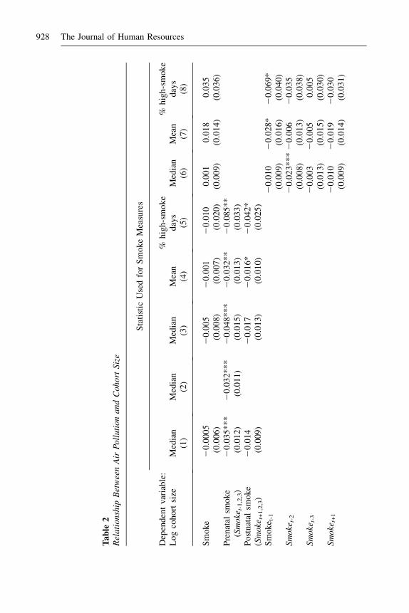
Table 2, Column 1, presents the relationship between cohort size and exposure tosmoke. The independent variables are Smoke, which is pollution in the month ofbirth, PrenatalSmoke which is pollution in the three months before birth, and Post-natalSmoke which is pollution in the three months after birth. Prenatal exposure topollution decreases the survival rate of fetuses, infants, and children: PrenatalSmokehas a coefficient of 20.035 that is statistically significant at the 1 percent level. Thecoefficient for Smoke is very close to zero, while the coefficient for PostnatalSmokeis 20.014 though statistically insignificant. Standard errors are clustered within anisland-month.10 In Column 2, when PrenatalSmoke is the only variable in the regres-sion (besides fixed effects), the coefficient is similar to that in Column 1.11

The regressions are weighted by population, but as a specification check, the un-weighted regression is shown in Column 3. The results are similar, with coefficientsand standard errors that are larger in magnitude. The larger standard errors suggestthat, given heteroskedasticity, weighting by population improves efficiency. Theother rationale for weighting is that the dependent variable measures proportionalrather than absolute changes in cohort size. Columns 4 and 5 consider alternative

10. The standard error for PrenatalSmoke is 0.014 if one clusters on island instead of island-month.11. See Appendix Table A2 for an instrumental variable estimate of the effect of PrenatalSmoke on cohortsize that uses only coarse variation in pollution. The instrument for PrenatalSmoke is a dummy for Kali-mantan or Sumatra interacted with a dummy for September 1997 to January 1998 (first stage F-statistic of45.6). The IV coefficient is 20.037.

Jayachandran 927

Ta

ble

2R

ela

tio

nsh

ipB

etw

een

Air

Po

llu

tio

na

nd

Co

ho

rtS

ize

Sta

tist

icU

sed

for

Sm

ok

eM

easu

res

Dep

end

ent

vari

able

:L

og

coh

ort

size

Med

ian

Med

ian

Med

ian

Mea

n%

hig

h-s

mo

ke

day

sM

edia

nM

ean

%h

igh

-sm

ok

ed

ays

(1)

(2)

(3)

(4)

(5)

(6)

(7)

(8)

Sm

ok

e2

0.0

00

52

0.0

05

20

.00

12

0.0

10

0.0

01

0.0

18

0.0

35

(0.0

06

)(0

.00

8)

(0.0

07

)(0

.02

0)

(0.0

09

)(0

.01

4)

(0.0

36

)P

ren

atal

smo

ke

(Sm

oke

t-1

,2,3

)2

0.0

35

**

*2

0.0

32

***

20

.04

8*

**

20

.03

2*

*2

0.0

85

**

(0.0

12

)(0

.01

1)

(0.0

15

)(0

.01

3)

(0.0

33

)P

ost

nat

alsm

ok

e2

0.0

14

20

.01

72

0.0

16

*2

0.0

42

*(S

mo

ket+

1,2

,3)

(0.0

09

)(0

.01

3)

(0.0

10

)(0

.02

5)

Sm

ok

e t-1

20

.01

02

0.0

28

*2

0.0

69

*(0

.00

9)

(0.0

16

)(0

.04

0)

Sm

oke

t-2

20

.02

3*

**

20

.00

62

0.0

35

(0.0

08

)(0

.01

3)

(0.0

38

)S

mo

ket-

32

0.0

03

20

.00

50

.00

5(0

.01

3)

(0.0

15

)(0

.03

0)

Sm

oke

t+1

20

.01

02

0.0

19

20

.03

0(0

.00

9)

(0.0

14

)(0

.03

1)


Sm

oke

t+2

20

.00

52

0.0

03

20

.03

4(0

.00

8)

(0.0

14

)(0

.03

4)

Sm

oke

t+3

0.0

01

20

.00

10

.01

0(0

.00

9)

(0.0

12

)(0

.03

1)

Ob

serv

atio

ns

67

,45

46

7,4

54

67

,45

46

7,4

54

67

,45

46

7,4

54

67

,45

46

7,4

54

Wei

gh

ted

?Y

YN

YY

YY

YS

ub

dis

tric

tan

dm

on

thF

Es?

YY

YY

YY

YY

Note

:E

ach

obse

rvat

ion

isa

subdis

tric

t-m

onth

.S

tandar

der

rors

,in

par

enth

eses

bel

owth

eco

effi

cien

ts,

allo

wfo

rcl

ust

erin

gat

the

isla

nd-m

onth

lev

el.*

**

indic

ates

p<

0.0

1;

**

indic

ates

p<

0.0

5,

*in

dic

ates

p<

0.1

0.

Obse

rvat

ions

are

wei

ghte

dby

the

num

ber

of

indiv

idual

sen

um

erat

edin

the

Cen

sus

who

resi

de

inth

esu

bdis

tric

tan

dw

ere

born

inth

eyea

rbef

ore

the

sam

ple

per

iod,

exce

pt

inC

olu

mn

3w

hic

his

unw

eighte

d.

Jayachandran 929

monthly pollution measures, first, the mean rather than median of the daily pollutionvalues and, second, the proportion of days with high pollution (aerosol index above0.75). Mean pollution gives nearly identical results as the median value, with post-natal exposure now having a negative impact on cohort size that is marginally signif-icant. For the proportion of days with high pollution, the point estimate implies thatwhen there are three additional high-smoke days in a month (an increase of ten per-centage points), cohort size decreases by 0.85 percent.

Exposure to pollution in utero is associated with a decrease in fetal, infant, and childsurvival. To assess the aggregate magnitude of the effect, note that PrenatalSmoke washigher by 0.30 during September 1997 to January 1998 compared to the same calendarmonths a year earlier; this five-month period are the cohorts for whom PrenatalSmokeincludes a month during the fires. Multiplying that gap by the coefficient of 20.035implies that the fires led to a 1.1 percent decrease in cohort size. A more precise wayto estimate the total effect is to use the coefficient for PrenatalSmoke and calculate whatthe population would have been for each subdistrict if during the period during and im-mediately after the fires, PrenatalSmoke had taken on its value from 12 months earlier.Aggregated over the five months for the 3,751 subdistricts, this calculation similarlyimplies a population decline of 1.2 percent, or 15,600 missing children.12 Indonesia’sbaseline under-3 mortality rate was roughly 60 per 1,000 live births at this time.13 If theeffect of pollution was due exclusively to infant and child deaths, the estimates wouldrepresent a 20 percent effect; if half of the effect was due to fetal deaths, the coefficientwould imply a 10 percent effect on under-three mortality.14

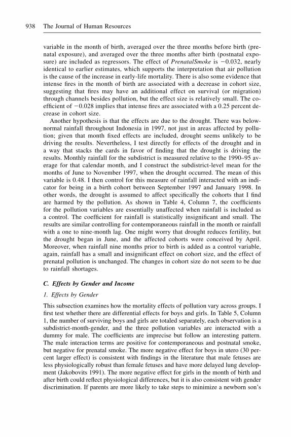
Figure 3 shows the nonparametric relationship between third-trimester exposureand cohort size. The effect of pollution is linear for the most part. There appearsto be a somewhat steeper relationship at high levels of pollution, but the nonlinear-ities are statistically insignificant when estimated parametrically with a spline or qua-dratic term.

The next regressions use the pollution level in each of the three months preceding andfollowing birth, rather than aggregated for a quarter. Table 2, Column 6, reports theresults using the median pollution level. For prenatal exposure (lags of Smoke), the ef-fect is strongest two months before the month of birth. For postnatal exposure (leads ofSmoke), the effect is strongest immediately after birth, though the estimates are impre-cise. The next two columns repeat the exercise using the month’s mean pollution andthe proportion of days that have high pollution. The general pattern of the coefficientsfor postnatal pollution remains the same, but the pattern for prenatal exposure changes.For the mean pollution level or number of high-smoke days (Columns 7 and 8), expo-sure in the month immediately before the month of birth now has the strongest negative

12. The estimates using high-smoke days imply a 1.0 percent aggregate effect. (The mean of the prenatalhigh-smoke variable is 0.131 during the 1997-98 episode and 0.006 for the same calendar months a yearearlier, and the coefficient in Table 2, Column 4, is 20.085.)13. The government estimates of under-one and under-five mortality rates at this time are 5 percent and 7percent, respectively. I assume that half of deaths between age one and five occur before age three.14. The welfare implications of pollution-induced mortality depend on how long individuals otherwisewould have lived. One can calculate using the child mortality rate that in the extreme ‘‘havesting’’ scenario,all deaths between ages three and six or seven would have to have been pushed forward to the time of thefires. Moreover, by most standards, the shortening of children’s lives by even a few years is a significantwelfare loss.


relationship with cohort size. One interpretation is that at different points during ges-tation, fetuses are more vulnerable to sustained exposure to pollution versus extremelevels of pollution. A more likely interpretation is that there is not enough precisionto determine at this level of detail how the timing of exposure affects survival.15 Thus,for the rest of the analysis, I focus on the three-month measures of prenatal and post-natal exposure. The results are similar using two-month measures.

B. Effect of Smoke on Mortality versus Alternative Hypotheses

The results in Table 2 suggest that exposure to smoke in utero causes early-life mor-tality. This section considers other possible explanations for the results.

1. Migration

The Census identifies respondents by their subdistrict of current residence, but expo-sure to pollution depends on where one resided during the fires. Migration could be a

Figure 3Kernel Regression of Log Cohort Size on Prenatal Exposure to PollutionNote: The solid line is the estimated relationship between log cohort size and pollution (PrenatalS-

moke). The dashed lines are the bootstrapped 95 percent confidence interval, with errors clustered

within an island-month. The model estimated is a locally weighted nonparametric regression of

log cohort size on pollution conditional on year and district fixed effects, following Robinson

(1988). Log cohort size has been offset by a constant so that its value is one at an aerosol index

of zero.

15. The month-by-month patterns, unlike the results with the three-month measures, are also somewhatsensitive to using a different sample period or a different threshold for high-smoke days.

Jayachandran 931

reason that cohorts with the highest prenatal exposure to pollution are smaller ifwomen in the third trimester of pregnancy were especially likely to migrate awayfrom high-pollution areas, either while pregnant or after giving birth. Fortunately,the Census collects data on the district (though not subdistrict) where an individualwas born and where he or she lived five years earlier, which enable one to probe thisconcern.16

To examine the extent of pollution-induced migration that occurs after birth, I re-peat the main analysis by district of birth. Cohort size is aggregated to the districtlevel, and the pollution measure for the district is a population-weighted averageof the subdistrict measure. The regression is weighted by the district population inthe two years prior to the sample period. For comparison, Column 1 of Table 3presents results by district of residence, and Column 2 presents results by districtof birth. The results are nearly identical to each other, as well as to the subdis-trict-level analysis, in terms of both point estimates and precision. Between-districtmigration after the birth of the infant is not the likely explanation for the relationshipbetween pollution and cohort size.

Pollution-induced migration also may take place before the infant is born. If somewomen spent most of their third trimester of pregnancy in the hardest-hit areas butmigrated away before giving birth, then neither place of residence in 2000 nor placeof birth would accurately reflect the fetus’s location during the fires. While the Cen-sus did not ask respondents where they resided in August to October 1997, it did askwhere they lived in 1995. As long as people do not migrate across districts repeat-edly, this measure should be a good proxy for where pollution-induced migrantslived at the time of the fires. To test for migration that occurs before birth, I matchinfants to their mothers as described in the data appendix and repeat the estimate bythe district where the mother resided in 1995. The results, shown in Column 3, areunchanged from the earlier estimates. In sum, migration, either before or after birth,does not seem to account for the negative relationship between exposure to pollutionand cohort size.17

2. Fertility

The empirical approach interprets decreases in ln(CohortSize) as increases in early-lifedeaths, but there would also be fewer survivors if the number of births decreased. Itseems unlikely that conceptions declined nine months before the fires with a spatialpattern matching the pollution, but this concern also can be tested more directly byconstructing a measure of predicted births. First, I measure the percentage of womenof each age who give birth, using a time period not in the sample (namely, the youn-gest cohorts in the Census, those born in 1999 and 2000). I then apply these birthrates to the demographic composition of each district-month in the sample. This

16. For 9 percent of the sample, district of residence differs from district of birth, for 7 percent it differsfrom mother’s residence five years earlier, and for 12 percent it differs from one or the other.17. Within-district migration is unlikely to be driving the results since there is very little within-districtvariation in pollution, and most of it derives from interpolation so is noisy. In a model with district-month fixed effects, the coefficient for PrenatalSmoke is 20.013, smaller than in the main specification(Table 2, Column 1), and imprecise, suggesting that between-district variation is dominant in the mainestimates.


gives a predicted number of births based on demographic shifts. (See the data appen-dix for further details.) Table 4, Column 1, shows the results when ln(PredictedBirths)is included as a control variable. The coefficient of survivors on births is predicted tobe slightly less than 1. Because the measure is noisy especially after conditioning onsubdistrict and month indicators, the estimate is likely to suffer from attenuation bias.The estimated coefficient on predicted births is less than but statistically indistinguish-able from 1. More importantly, the coefficients on the pollution variables are essen-tially unchanged with this control variable included. Fluctuations in fertility causedby demographic shifts do not appear to be a confounding factor in the analysis.18

3. Preterm Births

Another concern is that the missing children are not deaths but instead are an artifactof changes in gestation length. Exposure to pollution may have induced preterm de-livery which is often associated with traumatic pregnancies. The reason this mech-anism could conceivably generate the results is that it is prenatal exposure that has astrong negative relationship with cohort size. Consider August 1997, the month thefires started. Pollution levels were high in August, and the value of PrenatalSmokefor August is low since there was no significant smoke in May, June, or July. In

Table 3Distinguishing Between Mortality and Migration

District of Residence VersusBirthplace Versus Mother’s 1995 Residence

Dependent variable:Log cohort size Residence Birthplace

Mother’s 1995residence

(1) (2) (3)

Smoke 20.002 0.002 0.002(0.006) (0.006) (0.006)

Prenatal smoke 20.035*** 20.037*** 20.038***(0.012) (0.012) (0.012)

Postnatal smoke 20.013 20.015 20.016(0.010) (0.010) (0.010)

Observations 5,829 5,829 5,829Fixed effects month, district month, district month, district

Note: Each observation is a district-month. Standard errors, in parentheses below the coefficients, allow forclustering at the island-month level. *** indicates p < 0.01; ** indicates p < 0.05, * indicates p < 0.10.Observations are weighted by the number of individuals enumerated in the Census who reside in the districtand were born in the year before the sample period.

18. Appendix Table A3 addresses another potential concern about fertility, namely that the seasonality ofbirths or deaths could differ for areas more affected by the pollution, generating a spurious result. Theresults are robust to restricting the sample to the months with high PrenatalSmoke plus the same calendarmonths one year earlier.

Jayachandran 933

Ta

ble

4A

lter

nati

veH

ypoth

eses

Dep

end

ent

vari

able

:L

og

coh

ort

size

Co

ntr

ol

for

Pre

dic

ted

Fer

tili

tyE

xcl

ud

ing

Au

gu

st1

99

7

SU

SE

NA

San

dP

OD

ES

sub

sam

ple

Co

ntr

ol

for

Fin

anci

alC

risi

s

Ex

clu

din

gA

reas

wit

hF

ires

Co

ntr

ol

for

Fir

esC

on

tro

lfo

rR

ain

fall

(1)

(2)

(3)

(4)

(5)

(6)

(7)

Sm

ok

e0

.00

10

.00

10

.00

20

.00

20

.00

30

.00

40

.00

1(0

.00

6)

(0.0

06

)(0

.00

6)

(0.0

06

)(0

.01

1)

(0.0

06

)(0

.00

6)

Pre

nat

alS

mo

ke

20

.03

5*

**

20

.03

6*

**

20

.03

2*

**

20

.03

2*

**

20

.03

5*

*2

0.0

32

**

20

.03

2**

(0.0

12

)(0

.01

2)

(0.0

11

)(0

.01

1)

(0.0

18

)(0

.01

4)

0.0

13

Po

stn

atal

smo

ke

20

.01

42

0.0

09

20

.01

22

0.0

12

0.0

16

20

.00

52

0.0

14

(0.0

09

)(0

.01

0)

(0.0

09

)(0

.00

9)

(0.0

14

)(0

.01

1)

(0.0

09

)L

n(p

red

icte

db

irth

s)0

.87

5(0

.69

6)

Fin

anci

alcr

isis

20

.04

9(0

.03

8)

Any

fire

s2

0.0

04

(0.0

10

)P

ren

atal

any

fire

s0

.00

7(0

.01

7)

Po

stn

atal

any

fire

s2

0.0

04

(0.0

14

)In

ten

sefi

res

20

.02

8*

(0.0

16

)P

ren

atal

inte

nse

fire

s2

0.0

17

(0.0

25

)


Po

stn

atal

inte

nse

fire

s2

0.0

21

(0.0

29

)R

ain

fall

20

.02

3(0

.03

3)

Ob

serv

atio

ns

67

,45

46

3,7

03

63

,15

86

3,1

58

52

,64

66

7,4

54

67

,45

4S

ub

dis

tric

tan

dm

on

thF

Es?

YY

YY

YY

Y

Note

:E

ach

obse

rvat

ion

isa

subdis

tric

t-m

onth

.S

tandar

der

rors

,in

par

enth

eses

bel

owth

eco

effi

cien

ts,a

llow

for

clust

erin

gat

the

isla

nd-m

onth

leve

l.***

indic

ates

p<

0.0

1;

**

indic

ates

p<

0.0

5,

*in

dic

ates

p<

0.1

0.

Obse

rvat

ions

are

wei

ghte

dby

the

num

ber

of

indiv

idual

sen

um

erat

edin

the

Cen

sus

who

resi

de

inth

esu

bdis

tric

tan

dw

ere

born

inth

eyea

rbef

ore

the

sam

ple

per

iod.

Pre

dic

ted

Bir

ths

isco

nst

ruct

edusi

ng

the

fert

ilit

yra

teby

age

and

the

num

ber

of

wom

enof

dif

fere

nt

chil

d-b

eari

ng

ages

wit

hin

adis

tric

t,as

des

crib

edin

the

dat

aap

pen

dix

.T

he

finan

cial

cris

isva

riab

leis

stan

dar

diz

edto

hav

ea

mea

nof

0an

dst

andar

ddev

iati

on

of

1fo

rth

esa

mple

.A

reas

wit

hout

fire

sar

eth

ose

wit

hfe

wer

than

20

fire

-day

sov

erth

een

tire

per

iod.

Any

fire

sis

anin

dic

ator

of

any

fire

san

din

tense

fire

sis

anin

dic

ator

of

atle

ast

10

fire

-day

sin

the

month

.T

he

rain

fall

vari

able

issu

bdis

tric

t-le

vel

rain

fall

for

the

1997

dro

ught

month

sof

June

toN

ove

mber

div

ided

by

the

1990–95

aver

age

for

those

cale

ndar

month

s,in

tera

cted

wit

ha

dum

my

for

bei

ng

ina

bir

thco

hort

bet

wee

nS

epte

mber

1997

and

Januar

y1998.

Jayachandran 935

September, in contrast, PrenatalSmoke is high since it incorporates the pollution inAugust. If infants due in September were instead born in August, then births wouldhave shifted from a high-PrenatalSmoke month to a low-PrenatalSmoke month, gen-erating a negative relationship between PrenatalSmoke and cohort size that is unre-lated to mortality. To test the preterm-birth hypothesis, I repeat the analysis droppingAugust 1997 from the sample. If the above hypothesis were correct, the coefficienton PrenatalSmoke would become less negative compared to the baseline results. Asshown in Table 4, Column 2, this does not occur. The coefficients are nearly iden-tical between the full sample and the subsample, contrary to what one would expectif the pollution had induced preterm births but had not affected infant survival.19

The effect of pollution on cohort size is not due to preterm births instead of beingdue to fetal and infant deaths. Note, however, that pollution may have caused infantdeaths precisely by inducing premature births (which put infants at greater risk ofdeath); that is, preterm delivery is potentially an important channel through whichexposure to pollution led to mortality.

4. Financial Crisis

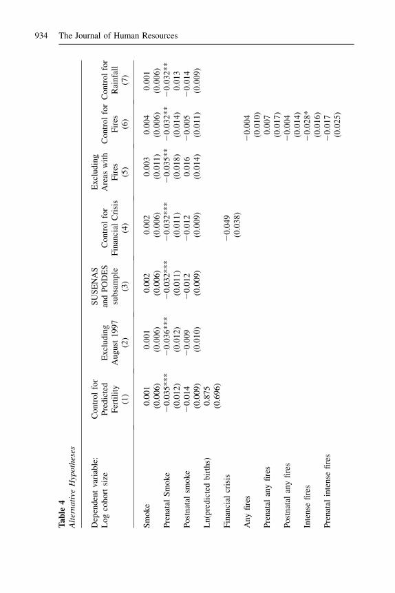
The Indonesian financial crisis began shortly after the fires, as shown in Figure 4. Toverify that the analysis is not attributing to air pollution deaths that were caused bythe crisis, a measure of the financial crisis is added to the model. No monthly sub-district-specific data on the crisis were collected, to my knowledge, so I construct ameasure of the crisis by interacting a cross-sectional measure, the inverse ratio ofmedian income (consumption) at the height of the crisis in 1999 to median incomebefore the crisis in 1996, and a time-series measure, the consumer price index forfood. The regression results can be anticipated by noting that the cross-sectional cor-relation between the crisis measure and pollution in September 1997 (peak of thefires) is 0.03; the spatial patterns of the crisis are not similar to the spatial patternsof pollution. For regressions that use variables from the SUSENAS or PODES sur-veys, a slightly smaller sample of subdistricts is used due to data availability. Table4, Column 3, shows the regression results for the baseline model and confirms thatthe subsample is similar to the full sample, with a coefficient on PrenatalSmoke of20.032. Column 4 then shows the results when the crisis measure for the monthof birth is included as a control variable. The estimated effect of PrenatalSmokeremains 20.032. The crisis measure has been normalized to have a mean of zeroand standard deviation of one for the sample, so the coefficient implies that a onestandard deviation increase in the crisis is associated with a 4.9 percent smaller co-hort, though the coefficient is statistically insignificant (and moreover could be due tomigration rather than mortality).20;21

19. Appendix Table 3 restricts or expands the sample to other time periods, and the results are robust to thischange. One noteworthy finding is that the estimated effect of PrenatalSmoke is smaller when the windowextends more than eight months after the fires, suggesting that the fires may have reduced fertility.20. Since the crisis accelerated a few months after the fires, I also estimated models that control for thecrisis measure for the three months following the month of birth. This generates more variation in the crisismeasure during the period of interest. The estimated effect of PrenatalSmoke is unchanged.21. Rukumnuaykit (2003) finds a 3 percent increase in infant mortality in 1997-98 in the Indonesia FamilyLife Survey, which is interpreted as due to the financial crisis, drought and smoke.


5. Effect of Pollution versus Effect of Fires or Drought

Another interpretation of the results is that they represent reduced-form effects ofthe fires rather than effects of specifically air pollution. The regressor is the pol-lution level, but the smoke affected places nearby the sites of fires, and the firescould have caused mortality through income effects, degraded food supply, andother channels. To separate the effect of pollution from other effects of the fires,I use data on where the fires occurred. I calculate the number of fire-days occur-ring in or near a subdistrict based on satellite data on ‘‘hot spot’’ locations anddurations. Firedays is the duration of each fire summed over all fires within 50km of the subdistrict center. First, I examine the effects of pollution in areas thatdid not experience extensive fires. In essence, the identification comes from firesin neighboring areas and the direction that the winds blew the pollution. In Table4, Column 5, the sample is restricted to subdistricts where fewer than 20 fire-daysoccurred over the sample period, which eliminates 22 percent of subdistricts, pre-dominantly in Kalimantan and Sumatra.22 The coefficient on PrenatalSmoke onlog cohort size remains 20.035 for these areas that experienced only the pollutionfrom the fires. Next, I include measures of fire prevalence as regressors. The fire-days variable is highly skewed, so I use two indicator variables, one for whetherthere were any fire-days in the subdistrict-month (sample mean of 0.16) and a sec-ond for whether there were intense fires, defined as at least ten fire-days during themonth (sample mean of 0.03). In Column 6, the fires variable and intense fires

Figure 4Timing of the Fires and the Financial Crisis

22. Because of measurement error in the hotspot data, eliminating any subdistrict with at least one fire-daywould eliminate more than two-thirds of subdistricts, which is inconsistent with the actual geographic ex-tent of the fires. Fewer than 22 percent of subdistricts were probably affected, so the results shown are con-servative. They are similar if other thresholds are chosen.

Jayachandran 937

variable in the month of birth, averaged over the three months before birth (pre-natal exposure), and averaged over the three months after birth (postnatal expo-sure) are included as regressors. The effect of PrenatalSmoke is 20.032, nearlyidentical to earlier estimates, which supports the interpretation that air pollutionis the cause of the increase in early-life mortality. There is also some evidence thatintense fires in the month of birth are associated with a decrease in cohort size,suggesting that fires may have an additional effect on survival (or migration)through channels besides pollution, but the effect size is relatively small. The co-efficient of 20.028 implies that intense fires are associated with a 0.25 percent de-crease in cohort size.

Another hypothesis is that the effects are due to the drought. There was below-normal rainfall throughout Indonesia in 1997, not just in areas affected by pollu-tion; given that month fixed effects are included, drought seems unlikely to bedriving the results. Nevertheless, I test directly for effects of the drought and ina way that stacks the cards in favor of finding that the drought is driving theresults. Monthly rainfall for the subdistrict is measured relative to the 1990–95 av-erage for that calendar month, and I construct the subdistrict-level mean for themonths of June to November 1997, when the drought occurred. The mean of thisvariable is 0.48. I then control for this measure of rainfall interacted with an indi-cator for being in a birth cohort between September 1997 and January 1998. Inother words, the drought is assumed to affect specifically the cohorts that I findare harmed by the pollution. As shown in Table 4, Column 7, the coefficientsfor the pollution variables are essentially unaffected when rainfall is included asa control. The coefficient for rainfall is statistically insignificant and small. Theresults are similar controlling for contemporaneous rainfall in the month or rainfallwith a one to nine-month lag. One might worry that drought reduces fertility, butthe drought began in June, and the affected cohorts were conceived by April.Moreover, when rainfall nine months prior to birth is added as a control variable,again, rainfall has a small and insignificant effect on cohort size, and the effect ofprenatal pollution is unchanged. The changes in cohort size do not seem to be dueto rainfall shortages.

C. Effects by Gender and Income

1. Effects by Gender

This subsection examines how the mortality effects of pollution vary across groups. Ifirst test whether there are differential effects for boys and girls. In Table 5, Column1, the number of surviving boys and girls are totaled separately, each observation is asubdistrict-month-gender, and the three pollution variables are interacted with adummy for male. The coefficients are imprecise but follow an interesting pattern.The male interaction terms are positive for contemporaneous and postnatal smoke,but negative for prenatal smoke. The more negative effect for boys in utero (30 per-cent larger effect) is consistent with findings in the literature that male fetuses areless physiologically robust than female fetuses and have more delayed lung develop-ment (Jakobovits 1991). The more negative effect for girls in the month of birth andafter birth could reflect physiological differences, but it is also consistent with genderdiscrimination. If parents are more likely to take steps to minimize a newborn son’s


exposure to pollution or to seek medical treatment for his respiratory infection, forexample, then one would expect the effects of postnatal pollution to be strongerfor girls. However, these interpretations should be treated with caution since the gen-der differences are not statistically significant.

2. Effects by Income

The next estimates test whether the effects of pollution are more pronounced inpoorer places. This type of heterogeneity could arise if the poor effectively are ex-posed to more pollution, for example, because they spend more time outdoors do-ing strenuous work or are less likely to evacuate the area. It could also arise if thesame amount of effective pollution leads to bigger health effects for the poor, forexample, because they have lower baseline health, making them more sensitive topollution, or have less access to healthcare to treat the health problems caused bythe pollution.

Column 2 of Table 5 uses food consumption as a proxy for income to examinethis hypothesis, interacting the pollution measures with a dummy variable forwhether the district’s median log consumption in 1996 is above the 50th percen-tile among all subdistricts. All three of Smoke, PrenatalSmoke, and Postnatal-Smoke are associated with smaller cohorts for the bottom half of theconsumption distribution, and the interaction terms for the top half of the distri-bution are large and positive. The weighted average of the coefficients for thebottom and top halves of the distribution would be more negative than the aver-age effect found earlier, however. The reason is that month effects vary with in-come. As has been documented in the demography literature, seasonality infertility tends to be stronger and qualitatively different in poorer areas (Lamand Miron 1991). Thus, Column 3 includes separate month fixed effects for thetop and bottom halves of the consumption distribution. The results are qualita-tively similar to those in Column 2. The effect of prenatal exposure is largeand negative when consumption is below the median. In these areas, postnatal ex-posure is also statistically significant, with an effect size about 60 percent that ofprenatal exposure. Each of the interaction coefficients for districts with abovemedian consumption is positive, and in the case of PrenatalSmoke, significantat the 1 percent level. The effect of a one unit change in PrenatalSmoke is20.06 for the top half of the distribution and 20.13, or over twice as large,for the bottom half. Average log consumption is 0.4 log points larger in thetop half of the distribution compared to the bottom half, so another way to viewthe results is that when consumption increases by 50 percent (e0.4), the effect sizedecreases by 50 percent.

The dependence of seasonal patterns on income suggests that including separatemonth effects for the two halves of the consumption distribution might be the pre-ferred specification even for estimating the average effect. In addition, for the rea-sons explained by Deaton (1995), given the heterogeneous effects, the averageeffect should be calculated by separately estimating the effect by consumptionlevel and then averaging. This amounts to averaging the coefficients in Column3, weighted by the population in each half of the consumption distribution. Asshown in Column 4, the average effect for prenatal smoke is then 20.090 and

Jayachandran 939

Ta

ble

5E

ffec

tsb

yG

end

era

nd

Inco

me

By

gen

der

By

inco

me

(lo

gco

nsu

mp

tio

n)

of

the

dis

tric

t

To

pq

uar

tile

3rd

qu

arti

le2

nd

qu

arti

leB

ott

om

qu

arti

leD

epen

den

tva

riab

le:

Lo

gco

ho

rtsi

ze(1

)(2

)(3

)(4

)(5

)

Sm

ok

e2

0.0

08

20

.06

0*

**

20

.02

42

0.0

13

20

.00

42

0.0

11

20

.02

80

.00

2(0

.00

7)

(0.0

21

)(0

.01

6)

(0.0

17

)(0

.00

9)

(0.0

10

)(0

.02

4)

(0.0

45

)P

ren

atal

smo

ke

20

.03

0**

20

.15

8*

**

20

.12

9*

**

20

.09

0**

*2

0.0

58

**

*2

0.0

76

**

*2

0.0

94

**2

0.1

21

**

(0.0

12

)(0

.03

7)

(0.0

28

)(0

.01

5)

(0.0

18

)(0

.01

7)

(0.0

47

)(0

.06

1)

Po

stn

atal

smo

ke

20

.01

9*

20

.15

8*

**

20

.04

7*

20

.03

5**

20

.02

52

0.0

40

**

*2

0.0

46

0.0

09

(0.0

10

)(0

.02

7)

(0.0

24

)(0

.01

9)

(0.0

16

)(0

.01

4)

(0.0

32

)(0

.05

2)

Mal

e0

.01

4**

*(0

.00

3)

Sm

ok

e*

mal

e0

.01

6**

*(0

.00

5)

Pre

nat

alsm

ok

e*

mal

e2

0.0

09

(0.0

07

)P

ost

nat

alsm

ok

e*

mal

e0

.01

0(0

.00

6)

Sm

ok

e*

hig

hco

nsu

mp

tio

n0

.06

6*

**

(0.0

21

)0

.01

7(0

.01

4)

Pre

nat

alsm

ok

e*

hig

hco

nsu

mp

tio

n0

.12

7*

**

(0.0

38

)0

.07

2*

**

(0.0

27

)


Po

stn

atal

smo

ke

*h

igh

con

sum

pti

on

0.1

61

**

*(0

.02

6)

0.0

17

(0.0

14

)

Ob

serv

atio

ns

13

4,7

34

63

,15

86

3,1

58

63

,15

86

3,1

58

Fix

edef

fect

sin

clu

ded

sub

dis

tric

t,m

on

thsu

bd

istr

ict,

mo

nth

sub

dis

tric

t,m

on

th*

hig

hco

ns.

sub

dis

tric

t,m

on

th*

hig

hco

ns.

sub

dis

tric

t,m

on

th*

qu

arti

leo

flo

gco

nsu

mp

tio

n

Note

:E

ach

obse

rvat

ion

isa

subdis

tric

t-m

onth

.S

tandar

der

rors

,in

par

enth

eses

bel

owth

eco

effi

cien

ts,

allo

wfo

rcl

ust

erin

gat

the

isla

nd-m

onth

leve

l.***

indic

ates

p<

0.0

1;

**

indic

ates

p<

0.0

5,

*in

dic

ates

p<

0.1

0.

Hig

hco

nsu

m.

isan

indic

ator

that

equal

s1

ifth

edis

tric

t’s

med

ian

log

food

consu

mpti

on

isab

ove

the

sam

ple

med

ian.

Obse

r-va

tions

are

wei

ghte

dby

the

num

ber

of

indiv

idual

sen

um

erat

edin

the

Cen

sus

who

resi

de

inth

esu

bdis

tric

tan

dw

ere

born

inth

eyea

rbef

ore

the

sam

ple

per

iod.

Colu

mn

4re

port

sth

eav

erag

eof

the

coef

fici

ents

inC

olu

mn

3,w

eighte

dby

the

popula

tion

inea

chhal

fof

the

consu

mpti

on

dis

trib

uti

on;

the

stan

dar

der

ror

and

the

join

tsi

gnifi

cance

of

the

linea

rco

mbin

atio

nof

coef

fici

ents

issh

own.

Jayachandran 941

the coefficient for postnatal smoke is 20.035, both considerably larger than seenearlier in Table 2.

Next, I further break down the income distribution into quartiles (and includemonth-quartile fixed effects). Column 5 shows the separate coefficients by quar-tile, estimated as one regression. The point estimate on PrenatalSmoke becomesmore negative moving from higher to lower quartiles. The results are not veryprecise, though, and the PrenatalSmoke coefficients for different quartiles arenot statistically distinguishable from one another. The coefficients for the othersmoke variables are also imprecise, especially for the bottom two quartiles, andthe point estimates do not monotonically decline with consumption. Above- ver-sus below-median consumption, as opposed to a linear interaction term, is there-fore used below to parsimoniously characterize the heterogeneous effects byincome.

3. Effects by Urbanization, Wood-Stove Use, Healthcare, and Mother’s Education

This subsection tests some hypotheses about why there is an income gradient in thehealth effects of pollution. The tests are merely suggestive because the measuresused could be correlated with omitted variables and data are available to test onlya limited number of hypotheses.

One possibility is that urban areas experience smaller effects from the firesthan rural areas, generating the heterogeneity by income. Urbanization would onlybe a proximate cause, but one might think that in urban areas, housing stock is lesspermeable, healthcare is better, there is less outdoor work, or there are more effectivepublic advisories urging people to stay indoors, for example. On the other hand,pollution from the fires may have been particularly noxious in cities where it mixedwith industrial pollution from cars and factories. Column 1 of Table 6 interactsthe pollution measures with the proportion of the subdistrict population that livesin urban localities (based on those born in the year before the sample period).Only the coefficients for PrenatalSmoke and its interaction terms are reported,but Smoke, PostnatalSmoke, and their interactions are also included in the regres-sions. The effects of pollution do not vary by urbanization level, suggesting thatthe effects described above may have offset each other. In unreported results, Ialso find that children whose mothers work in agriculture do not experience largereffects.

Next I test whether the effects depend on the prevalence of wood-burning stoves.If the health impact of pollution is convex in exposure, those who have daily expo-sure to indoor air pollution could suffer more acutely from the wildfires. Foreach village or town, data are available on whether the majority of people usedwood or other biomass as their primary cooking fuel in 1996. I construct for eachsubdistrict the population-weighted average of this measure, which serves as acrude measure of the proportion of people in the subdistrict who use wood as theircooking fuel. The mean of the variable is 0.64. As shown in Column 2 of Table 6,wood fuel use is strongly associated with more negative effects from any givenlevel of exposure to the wildfire smoke. A 20 percentage point decrease in woodfuel use reduces the net effect of prenatal pollution by 0.03. By comparison, movingfrom the bottom half to the top half of the consumption distribution (50 percent


Ta

ble

6E

ffec

tsB

yU

rbaniz

ati

on,

Wood

Fuel

Use

,and

Hea

lthca

reSec

tor

Dep

enden

tva

riab

le:

log

cohort

size

(1)

(2)

(3)

(4)

(5)

Pre

nat

alsm

ok

e2

0.1

21

**

*0

.01

52

0.1

15

**

*2

0.1

13

**

*2

0.0

07

(0.0

28

)(0

.03

2)

(0.0

27

)(0

.02

8)

(0.0

25

)P

ren

atal

smo

ke

*u

rban

izat

ion

20

.01

3(0

.01

3)

Pre

nat

alsm

ok

e*

wo

od

fuel

use

20

.15

5*

**

20

.12

0*

**

(0.0

36

)(0

.02

6)

Pre

nat

alsm

ok

e*

mat

ern

ity

clin

ic0

.03

0*

**

0.0

11

**

(0.0

09

)(0

.00

5)

Pre

nat

alsm

ok

e*

do

cto

rs0

.04

8*

**

0.0

16

(0.0

15

)(0

.01

3)

Pre

nat

alsm

ok

e*

hig

hco

nsu

mp

tio

n0

.07

1*

**

0.0

48

*0

.05

8*

*0

.05

2*

*0

.04

4*

(0.0

27

)(0

.02

5)

(0.0

25

)(0

.02

5)

(0.0

25

)O

bse

rvat

ion

s6

3,1

58

63

,15

86

3,1

58

63

,15

86

3,1

58

Subdis

tric

tan

dm

onth

FE

s?Y

YY

YY

Note

:E

ach

obse

rvat

ion

isa

subdis

tric

t-m

onth

.S

tandar

der

rors

,in

par

enth

eses

bel

owth

eco

effi

cien

ts,a

llow

for

clust

erin

gat

the

isla

nd-m

onth

leve

l.***

indic

ates

p<

0.0

1;

**

indic

ates

p<

0.0

5,

*in

dic

ates

p<

0.1

0.

All

regre

ssio

ns

also

incl

ude

Sm

oke

and

Post

nat

alS

moke

and

thei

rin

tera

ctio

ns

wit

hth

ere

leva

nt

vari

able

sfo

rea

chco

lum

n.

Urb

aniz

atio

nis

the

pro

port

ion

of

the

popula

tion

inurb

anlo

cali

ties

and

isbas

edon

1994

to1996

bir

thco

hort

s.W

ood

fuel

use

isan

appro

xim

ate

mea

sure

of

the

pro

port

ion

of

peo

ple

inth

esu

bdis

tric

tw

ho

cook

wit

hw

ood

fuel

rath

erth

anker

ose

ne

and

gas

.H

ealt

hva

riab

les

are

norm

aliz

edto

be

mea

nze

ro,st

andar

ddev

iati

on

one

for

the

sam

ple

.H

igh

consu

mpti

on

isan

indic

ator

that

equal

sone

ifth

edis

tric

t’s

med

ian

log

food

consu

mpti

on

isab

ove

the

sam

ple

med

ian.

Obse

rvat

ions

are

wei

ghte

db

yth

enum

ber

of

indiv

idual

sen

um

erat

edin

the

Cen

sus

who

resi

de

inth

esu

bdis

tric

tan

dw

ere

born

inth

eyea

rbef

ore

the

sam

ple

per

iod.

Jayachandran 943

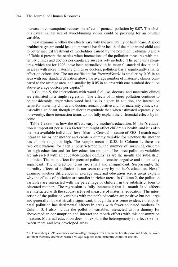
increase in consumption) reduces the effect of prenatal pollution by 0.07. The obvi-ous caveat is that use of wood-burning stoves could be proxying for an omittedvariable.

I next examine whether the effects vary with the availability of healthcare. A goodhealthcare system could lead to improved baseline health of the mother and child andto better medical treatment of morbidities caused by the pollution. Columns 3 and 4of Table 6 present the results when interactions of the pollution measures with ma-ternity clinics and doctors per capita are successively included. The per capita meas-ures, which are for 1996, have been normalized to be mean 0, standard deviation 1.In areas with more maternity clinics or doctors, pollution has a significantly smallereffect on cohort size. The net coefficient for PrenatalSmoke is smaller by 0.03 in anarea with one standard deviation above the average number of maternity clinics com-pared to the average area, and smaller by 0.05 in an area with one standard deviationabove average doctors per capita.23

In Column 5, the interactions with wood fuel use, doctors, and maternity clinicsare estimated in a single regression. The effects of in utero pollution continue tobe considerably larger when wood fuel use is higher. In addition, the interactionterms for maternity clinics and doctors remain positive and, for maternity clinics, sta-tistically significant, though smaller in magnitude than when estimated separately. Asnoteworthy, these interaction terms do not fully explain the differential effects by in-come.

Table 7 examines how the effects vary by mother’s education. Mother’s educa-tion is important per se as a factor that might affect children’s health, and it is alsothe best available individual-level (that is, Census) measure of SES. I match eachinfant to his or her mother and create a dummy variable for whether the motherhas completed junior high. The sample mean is 0.38. In Column 1, there aretwo observations for each subdistrict-month, the number of surviving childrenfor high-education and for low-education mothers. The three pollution variablesare interacted with an educated-mother dummy, as are the month and subdistrictdummies. The main effect for prenatal pollution remains negative and statisticallysignificant. The interaction terms are small and insignificant. Surprisingly, themortality effects of pollution do not seem to vary by mother’s education. Next Iexamine whether differences in average maternal education across areas explainwhy the effects of pollution are smaller in richer areas. In Column 2, the pollutionvariables are interacted with the percentage of children in the subdistrict born toeducated mothers. The regression is fully interacted; that is, month fixed effectsare interacted with the subdistrict-level measure of maternal education. The inter-action of the pollution variables with mother’s education are positive but not largeand generally not statistically significant, though there is some evidence that post-natal pollution has detrimental effects in areas with fewer educated mothers. InColumn 3, I also include the pollution variables interacted with a dummy forabove-median consumption and interact the month effects with this consumptionmeasure. Maternal education does not explain the heterogeneity in effect size be-tween more and less developed areas.

23. Frankenberg (1995) examines within-village changes over time in the health sector and finds that over-all infant mortality decreases when a village acquires more maternity clinics or doctors.


Table 7Effects by Mother’s Education

Measure of Mother’s Education

Dependent variable:Log cohort size

Individual-Specific

Subdistrict Average

(1) (2) (3)

Smoke 0.002 20.004 20.0130.007 0.012 (0.017)

Prenatal smoke 20.041*** 20.054*** 20.113***(0.013) (0.018) (0.029)

Postnatal smoke 20.010 20.036** 20.044(0.012) (0.018) (0.028)

Smoke * educated mother 20.007(0.005)

Prenatal smoke *educated mother

0.007(0.008)

Postnatal smoke *educated mother

20.010(0.009)

Smoke * percenteducated mothers

0.003(0.020)

20.009(0.020)

Prenatal smoke *percent educated mothers

0.021(0.029)

20.034(0.028)

Postnatal smoke *percent educated mothers

0.057*(0.034)

0.053*(0.034)

Smoke * highconsumption

0.018(0.014)

Prenatal smoke *high consumption

0.099***(0.026)

Postnatal smoke *high consumption

0.011(0.034)

Observations 134,908 63,158 63,158Fixed effects

includedsubdistrict *

educatedmother,month *educatedmother

subdistrict,month * %educatedmothers

subdistrict,month *

high consum.,month *

% educatedmothers

Note: Standard errors, in parentheses below the coefficients, allow for clustering at the island-month level.*** indicates p < 0.01; ** indicates p < 0.05, * indicates p < 0.10. In Column 1, each observation is a subdis-trict-month-education category. Educated mothers are defined as those who have completed junior high. In Col-umns 2 and 3, each cell is a subdistrict-month, and percent educated mothers is the subdistrict average over thesample period. When interacted with month fixed effects, percent educated is standardized to mean 0. High con-sumption is an indicator that equals 1 if the district’s median log food consumption is above the sample median.

Jayachandran 945

The factors examined are unable to fully explain why prenatal exposure to pol-lution has a smaller effect on mortality in higher income areas. Even after control-ling for wood-stove pollution, access to healthcare, and maternal education, thereremains a positive coefficient for the interaction of pollution and high consumption.With better measures of indoor pollution, healthcare, and parental education, onemight be able to explain more of the heterogeneity by income. There are also sev-eral channels not tested here. Mothers and newborns in poor areas might be lesshealthy to begin with because of poor nutrition. Dwellings in poor areas mightbe more permeable to smoke, allowing pollution from the wildfires to contaminateindoor air quality. Behavioral responses might differ by income, with those inricher areas being more likely to stay indoors, avoid strenuous activity, or tempo-rarily evacuate to less affected areas, for example.24 But regardless of the underly-ing causes, the findings suggest that the mortality costs of pollution aredisproportionately borne by the poor.25

V. Conclusion

Air pollution from land fires that engulfed Indonesia in late 1997 ledto over 15,600 child, infant, and fetal deaths, or a 1.2 percentage point decrease insurvival for the affected cohorts. This paper uses the abrupt timing of the pollutionand the spatial variation across Indonesia to identify these effects. The paper presentsevidence on the timing of exposure that is most harmful: in utero exposure to pollu-tion has the largest effect on survival. At levels that are common both indoors andoutdoors in many poor countries, particulate matter has a sizeable effect on early-lifemortality.

Questions in developing countries sometimes go unstudied because data are notavailable. Research on infant mortality effects of air pollution in the United Statesmakes use of linked natality-mortality records and ground-based pollution moni-tors. No such data exist for Indonesia. To overcome this obstacle, this paper usesan unconventional methodology. First, child, infant and fetal death are inferredfrom ‘‘missing children’’ in the 2000 Indonesian Census. While the indirectmethod could introduce potential problems, the paper is able to show that migra-tion, changes in gestation length, and other potential concerns do not seem to be

24. In unreported results, the effect of prenatal smoke is smaller in areas where more houses are con-structed with bricks and concrete (compared to wood, palm leaves, etc.). Worse road quality, which couldbe a proxy for higher costs of evacuating, is also associated with larger mortality effects of pollution. An-other approach to measuring evacuation would be to use distance to the nearest low-smoke area, but in prac-tice this variable is too highly correlated with the pollution level to be useful as an interaction term. Use ofsurgical masks might also vary with income. Kunii et al. (2002) surveyed 532 people during the fires andfound that use of surgical masks was associated with fewer respiratory problems, but most medical expertsbelieve that surgical masks are ineffective at blocking out fine particles.25. The income gradient in health for survivors could go in the same direction or, if the weakest individ-uals were ‘‘harvested,’’ in the opposite direction. Also, note that if richer people have less severe healtheffects because they are spending more money on healthcare or smokeless cooking stoves, then the in-come gradient in the welfare effects of pollution might be smaller than the income gradient in the healtheffects.


driving the results. Second, smoke data from a satellite-based spectrometer areused in lieu of ground-monitor pollution data. Because of the satellite’s global cov-erage, proxy measures of particulate matter are available for even remote, underde-veloped areas.

There are at least two broader lessons about environmental issues in developingcountries worth highlighting. First, environmental damage—and the accompanyinghealth effects—are yet another consequence of weak governance. Corruption, whichis prevalent in Indonesia as in many low–income countries, was an important factorbehind the catastrophic fires. The Suharto government turned a blind eye when largefirms started fires in violation of the law. The Minister of Forestry did try to holdfirms accountable. In September 1997 he named 176 firms suspected of illegally sett-ing fires. However, he quickly lost his job. Suharto, in a move that was brazen evenby his formidable standards of crony capitalism, installed his golfing partnerBob Hasan—a timber magnate—as the new Minister of Forestry in early 1998.Hasan was outspoken in blaming small farmers for the fires and exonerating largefirms, including his own. In virtually no cases were firms punished for starting illegalblazes.

The findings of the paper highlight a second link between the environment andeconomic development: the health burden from pollution seems to fall disproportion-ately on the poor. The estimated effect size is much larger in poorer areas than inricher areas. There is suggestive evidence that the heterogeneity could be due to peo-ple in underdeveloped areas using wood-burning stoves and facing a compoundedeffect of indoor plus outdoor air pollution. Differences in access to healthcare alsoseem to play a part. An interesting direction for further research would be to comparethe early-life mortality effects in richer neighboring countries that were affected byIndonesia’s pollution such as Malaysia and Singapore. Why the health effects of pol-lution vary with income remains an open question—and an area to pursue to betterunderstand how environmental degradation creates unique challenges in developingcountries.

Appendix 1

Verification That Census Counts Track Infant Mortality

This section verifies that population counts from the Census track data on births andinfant deaths from the 2002 Demographic and Health Survey (DHS). The log of thenumber of surviving children should increase one-for-one with the log of total birthsand decrease one-for-one with the infant mortality rate (as can be derived with a fewsteps of algebra). Thus, I estimate

lnðCohortSizeÞJT ¼ a + g1lnðBirthsÞJT + g2IMRJT + eJTð3Þ

where J is a province and T is a quarter, Births is the number of children born in theprovince-quarter, and IMR (infant mortality rate) is the fraction of those children whodied by June 2000 when the Census was taken. Very few births per subdistrict-monthare sampled in the DHS, so the validation exercise aggregates to provinces and

Jayachandran 947

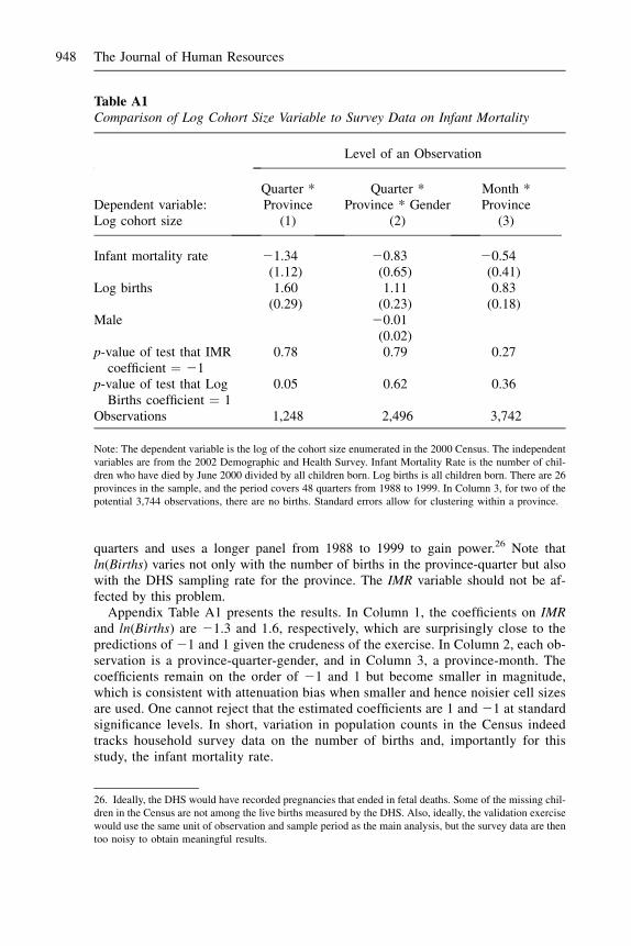
quarters and uses a longer panel from 1988 to 1999 to gain power.26 Note thatln(Births) varies not only with the number of births in the province-quarter but alsowith the DHS sampling rate for the province. The IMR variable should not be af-fected by this problem.

Appendix Table A1 presents the results. In Column 1, the coefficients on IMRand ln(Births) are 21.3 and 1.6, respectively, which are surprisingly close to thepredictions of 21 and 1 given the crudeness of the exercise. In Column 2, each ob-servation is a province-quarter-gender, and in Column 3, a province-month. Thecoefficients remain on the order of 21 and 1 but become smaller in magnitude,which is consistent with attenuation bias when smaller and hence noisier cell sizesare used. One cannot reject that the estimated coefficients are 1 and 21 at standardsignificance levels. In short, variation in population counts in the Census indeedtracks household survey data on the number of births and, importantly for thisstudy, the infant mortality rate.

Table A1Comparison of Log Cohort Size Variable to Survey Data on Infant Mortality

Level of an Observation

Dependent variable:Log cohort size

Quarter *Province

(1)

Quarter *Province * Gender

(2)

Month *Province

(3)

Infant mortality rate 21.34 20.83 20.54(1.12) (0.65) (0.41)

Log births 1.60 1.11 0.83(0.29) (0.23) (0.18)

Male 20.01(0.02)

p-value of test that IMRcoefficient ¼ 21

0.78 0.79 0.27

p-value of test that LogBirths coefficient ¼ 1

0.05 0.62 0.36

Observations 1,248 2,496 3,742

Note: The dependent variable is the log of the cohort size enumerated in the 2000 Census. The independentvariables are from the 2002 Demographic and Health Survey. Infant Mortality Rate is the number of chil-dren who have died by June 2000 divided by all children born. Log births is all children born. There are 26provinces in the sample, and the period covers 48 quarters from 1988 to 1999. In Column 3, for two of thepotential 3,744 observations, there are no births. Standard errors allow for clustering within a province.

26. Ideally, the DHS would have recorded pregnancies that ended in fetal deaths. Some of the missing chil-dren in the Census are not among the live births measured by the DHS. Also, ideally, the validation exercisewould use the same unit of observation and sample period as the main analysis, but the survey data are thentoo noisy to obtain meaningful results.


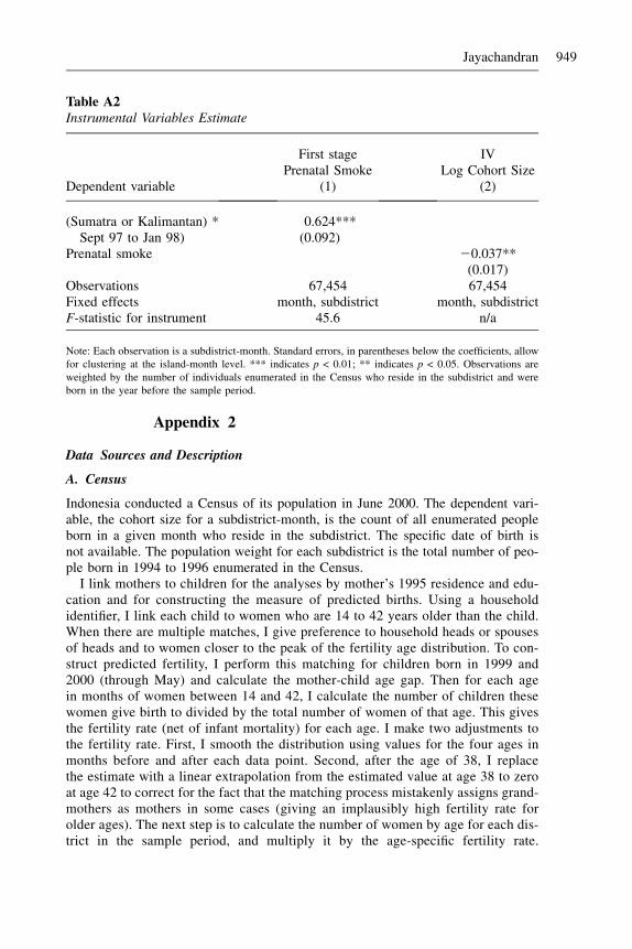
Appendix 2

Data Sources and Description

A. Census

Indonesia conducted a Census of its population in June 2000. The dependent vari-able, the cohort size for a subdistrict-month, is the count of all enumerated peopleborn in a given month who reside in the subdistrict. The specific date of birth isnot available. The population weight for each subdistrict is the total number of peo-ple born in 1994 to 1996 enumerated in the Census.

I link mothers to children for the analyses by mother’s 1995 residence and edu-cation and for constructing the measure of predicted births. Using a householdidentifier, I link each child to women who are 14 to 42 years older than the child.When there are multiple matches, I give preference to household heads or spousesof heads and to women closer to the peak of the fertility age distribution. To con-struct predicted fertility, I perform this matching for children born in 1999 and2000 (through May) and calculate the mother-child age gap. Then for each agein months of women between 14 and 42, I calculate the number of children thesewomen give birth to divided by the total number of women of that age. This givesthe fertility rate (net of infant mortality) for each age. I make two adjustments tothe fertility rate. First, I smooth the distribution using values for the four ages inmonths before and after each data point. Second, after the age of 38, I replacethe estimate with a linear extrapolation from the estimated value at age 38 to zeroat age 42 to correct for the fact that the matching process mistakenly assigns grand-mothers as mothers in some cases (giving an implausibly high fertility rate forolder ages). The next step is to calculate the number of women by age for each dis-trict in the sample period, and multiply it by the age-specific fertility rate.

Table A2Instrumental Variables Estimate

First stage IVPrenatal Smoke Log Cohort Size

Dependent variable (1) (2)

(Sumatra or Kalimantan) *Sept 97 to Jan 98)

0.624***(0.092)

Prenatal smoke 20.037**(0.017)

Observations 67,454 67,454Fixed effects month, subdistrict month, subdistrictF-statistic for instrument 45.6 n/a

Note: Each observation is a subdistrict-month. Standard errors, in parentheses below the coefficients, allowfor clustering at the island-month level. *** indicates p < 0.01; ** indicates p < 0.05. Observations areweighted by the number of individuals enumerated in the Census who reside in the subdistrict and wereborn in the year before the sample period.

Jayachandran 949

Ta

ble

A3

Dif

fere

nt

Sa

mp

leP

erio

ds

Sh

ort

erP

erio

ds

Bal

ance

dC

alen

dar

Mo

nth

sL

on

ger

Per

iod

Dep

enden

tva

riab

le:

log

cohort

size

3/9

7-

5/9

8(1

)1

2/9

6-

2/9

8(2

)3

/97

-2

/98

(3)

11

/96

-2

/97

&1

0/9

7-

2/9

8(4

)

11

/96

-2/9

7&

11

/97

-2

/98

(5)

12

/96

-5

/98

(6)

Sm

ok

e2

0.0

03

20

.00

42

0.0

09

*2

0.0

05

20

.02

12

0.0

01

(0.0

05

)(0

.00

5)

(0.0

05

)(0

.00

9)

(0.0

42

)(0

.00

6)

Pre

nat

alsm

ok

e2

0.0

43

**

*2

0.0

36

**

*2

0.0

49

**

*2

0.0

26

*2

0.0

30

**

20

.02

6*

*(0

.01

2)

(0.0

12

)(0

.01

2)

(0.0

14

)(0

.01

4)

(0.0

12

)P

ost

nat

alsm

ok

e2

0.0

23

**

*2

0.0

12

20

.02

6*

**

0.0

25

0.0

38

20

.00

6(0

.00

9)

(0.0

10

)(0

.00

8)

(0.0

30

)(0

.03

2)

(0.0

09

)O

bse

rvat

ion

s5

6,2

20

56

,20

14

4,9

67

33

,68

42

9,9

33

78

,70

3S

ubdis

tric

t&

mo

nth

FE

s?Y

YY

YY

Y

Note

:E

ach

obse

rvat

ion

isa

subdis

tric

t-m

onth

.S

tandar

der

rors

,in

par

enth

eses

bel

owth

eco

effi

cien

ts,

allo

wfo

rcl

ust

erin

gat

the

isla

nd-m

onth

leve

l.***

indic

ates

p<

0.0

1;

**

indic

ates

p<

0.0

5,

*in

dic

ates

p<

0.1

0.

Obse

rvat

ions

are

wei

ghte

dby

the

num

ber

of

indiv

idual

sen

um

erat

edin

the

Cen

sus

who

resi

de

inth

esu

bdis

tric

tan

dw

ere

born

inth

eyea

rbef

ore

the

bas

elin

esa

mple

per

iod.


Summing across all the ages of women of childbearing age gives the predictednumber of births for each district-month in the sample.

B. TOMS Pollution

In addition to the information provided in the text, further details on the Total OzoneMapping Spectrometer can be found at http://toms.gsfc.nasa.gov.

C. Fire Location and Rainfall

The European Space Agency compiles the ATSR World Fire Atlas, a list of ‘‘hot spots’’(date, time, latitude, and longitude) identified by nighttime infrared measurementsby the ATSR-2 instrument onboard the ERS-2 satellite. A hot spot corresponds to areading of > 312 Kelvins at 3.7 micron wavelength. For each subdistrict-month, hotspot-days within 50 km of the subdistrict’s center are used to calculate the numberof fire-days, or the sum over discrete fires of the duration of the fire in days.

The rainfall data set, Terrestrial Air Temperature and Precipitation: Monthly and An-nual Time Series, is from the Center for Climatic Research, University of Delaware.The rainfall measure for each node on a 0.5 degree latitude by 0.5 degree longitude gridis interpolated from 20 nearby weather stations using a spherical version of Shepard’sdistance-weighting method. The rainfall measure for a subdistrict uses the closest node.

D. SUSENAS

I use household level data from the 1996 and 1999 SUSENAS core modules, whichaggregate item-by-item consumption data to two categories, food and nonfood.For each household, per capita consumption is calculated weighting children by 0.75and infants by 0.6 compared to adults who are weighted by 1. The district log con-sumption measure is the median across all households of log food consumption percapita. The survey is representative at the district level, so I use district-level measures.

E. PODES

The PODES is a census of all villages and towns in Indonesia. I use population, fueluse, and health facilities questions for 1996. One question asks what cooking fuel themajority of the village uses, and I group the answers as wood fuel (wood plus otherbiomass) or other (kerosene and gas). The population-weighted average of this indi-cator variable across villages in a subdistrict is the fuel-use variable. Healthcaremeasures are unweighted per capita measures for the subdistrict, for the reason thatpeople have access to facilities throughout the subdistrict.

References

Almond, Douglas. 2006. ‘‘Is the 1918 Influenza Pandemic Over? Long-Term Effects of InUtero Influenza Exposure in the Post-1940 U.S. Population.’’ Journal of Political Economy114(3):672–712.

Jayachandran 951

Barber, Charles, and James Schweithhelm. 2000. Trial by Fire: Forest Fires and ForestryPolicy in Indonesia’s Era of Crisis and Reform. Washington, D.C.: World ResourcesInstitute.

Barker, David. 1990. ‘‘The Fetal and Infant Origins of Adult Disease.’’ British MedicalJournal 301, 1111.

Berkowitz, Gertrude, Mary Wolff, Teresa Janevic, Ian Holzman, Rachel Yehuda, and PhillipLandrigan. 2003. ‘‘The World Trade Center Disaster and Intrauterine Growth Restriction.’’Journal of the American Medical Association 290(5):595–96.

Bobak, Martin, and David Leon. 1992. ‘‘Air Pollution and Infant Mortality in the CzechRepublic, 1986-1988.’’ Lancet 340:1010–14.

Case, Anne, Darren Lubotsky, and Christina Paxson. 2002. ‘‘Economic Status and Healthin Childhood: The Origins of the Gradient.’’ American Economic Review 92(5):1308–34.

Chay, Kenneth, and Michael Greenstone. 2003a. ‘‘Air Quality, Infant Mortality, and theClean Air Act of 1970.’’ National Bureau of Economic Research Working Paper No.10053.

Chay, Kenneth, and Michael Greenstone. 2003b. ‘‘The Impact of Air Pollution on InfantMortality: Evidence from Geographic Variation in Pollution Shocks Induced by aRecession.’’ Quarterly Journal of Economics 118(3):1121–67.

Currie, Janet, and Rosemary Hyson. 1999. ‘‘Is the Impact of Health Shocks Cushioned bySocioeconomic Status? The Case of Low Birthweight.’’ American Economic Review89(2):245–50.

Currie, Janet, and Matthew Neidell. 2005. ‘‘Air Pollution and Infant Health: What Can WeLearn from California’s Recent Experience?’’ Quarterly Journal of Economics120(3):1003–30.

Deaton, Angus. 1995. ‘‘Data and Econometric Tools for Development Analysis.’’ inHandbook of Development Economics, Volume III, ed. Jere Berhman, and T. N. Srinivasan,1785–1882. Amsterdam: Elsevier.

Dejmek, Jan, Sherry Selevan, Ivan Benes, Ivo Solansky, and Radim Sram. 1999. ‘‘FetalGrowth and Maternal Exposure to Particulate Matter During Pregnancy.’’ EnvironmentalHealth Perspectives 107:475–80.

Donald, Stephen, and Kevin Lang. 2007. ‘‘Inference with Difference–in–Differences andOther Panel Data.’’ Review of Economics and Statistics 89(2):221–33.

Emmanuel, Shanta. 2000. ‘‘Impact to Lung Health of Haze from Forest Fires: The SingaporeExperience.’’ Respirology 5(2):175–82.

Ezzati, Majid and Daniel Kammen. 2002. ‘‘The Health Impacts of Exposure to Indoor AirPollution from Solid Fuels in Developing Countries: Knowledge, Gaps, and Data Needs.’’Environmental Health Perspectives 110(11):1–12.

Frankenberg, Elizabeth. 1995. ‘‘The Effects of Access to Health Care on Infant Mortality inIndonesia.’’ Health Transition Review 5:143–63.

Frankenberg, Elizabeth, Douglas McKee, and Duncan Thomas. 2004. ‘‘Health Consequencesof Forest Fires in Indonesia.’’ Demography 42(1):109–29.

Friedman, Michael, Kenneth Powell, Lori Hutwagner, LeRoy Graham, and W. Gerald Teague.2001. ‘‘Impact of Changes in Transportation and Commuting Behaviors During the 1996Summer Olympic Games in Atlanta on Air Quality and Childhood Asthma.’’ Journal of theAmerican Medical Association 285:897–905.

Hatch, Maureen, Dorothy Warburton, and Regina Santella. 1990. ‘‘Polycyclic AromaticHydrocarbon-DNA Adducts in Spontaneously Aborted Fetal Tissue.’’ Carcinogenesis11:1673–75.

Heil, Angelika, and Johan Goldammer. 2001. ‘‘Smoke-Haze Pollution: A Review of the 1997Episode in Southeast Asia.’’ Regional Environmental Change 2(1):24–37.


Her Majesty’s Public Health Service. 1954. ‘‘Mortality and Morbidity During the London Fogof December 1952.’’ Reports on Public Health and Medical Subjects.

Hsu, N. Christina, Jay Herman, Omar Torres, and Brent Holben. 1999. ‘‘Comparisons of theTOMS Aerosol Index with Sunphotometer Aerosol Optical Thickness: Results andApplications.’’ Journal of Geophysical Research 104:6269–80.

Hueglin, Christoph, Christian Gaegauf, Simon Kunzel, and Heinz Burtscher. 1997.‘‘Characterization of Wood Combustion Particles: Morphology, Mobility and PhotoelectricActivity.’’ Environmental Science and Technology 31:3439–47.

Jakobovits, Akos A. 1991. ‘‘Sex Ratio of Spontaneously Aborted Fetuses and DeliveredNeonates in Second Trimester.’’ European Journal of Obstetrics and Gynecology andReproductive Biology 40:211–13.

Kunii, Osamu, Shuzo Kanagawa, Iwao Yajima, Yoshiharu Hisamatsu, Sombo Yamamura,Takasi Amagai, and Ir Ismail. 2002. ‘‘The 1997 Haze Disaster in Indonesia: Its Air Qualityand Health Effects.’’ Archives of Environmental Health 57:16–22.

Lam, David, and Jeffrey Miron. 1991. ‘‘Seasonality of Births in Human Populations.’’ SocialBiology 38(1-2):51–77.

Lleras-Muney, Adriana. 2006. ‘‘The Needs of the Army: Using Compulsory Relocation in theMilitary to Estimate the Effect of Air Pollutants on Childrens Health.’’ Princeton, N.J.:Princeton University. Unpublished.

Loomis, Dana, Margarita Castillejos, Diane Gold, William McDonnell, and Victor Borja-Aburto. 1999. ‘‘Air Pollution and Infant Mortality in Mexico City.’’ Epidemiology 10:118–23.

MacKenzie, Karen, and D. Murray Angevine. 1981. ‘‘Infertility in Mice Exposed In Utero toBenzo½a�pyrene.’’ Biology of Reproduction 24:83–191.

Marmot, Michael D., George D. Smith, Stephen Stansfeld, Chandra Patel, Fiona North, J.Head, Ian White, Eric Brunner, and Amanda Feeney. 1991. ‘‘Health Inequalities amongBritish Civil Servants: The Whitehall II Study.’’ Lancet 1387–93.

Murphy, Kevin, and Robert Topel. 2006. ‘‘The Value of Health and Longevity.’’ Journal ofPolitical Economy 114(5):871–904.

Ostermann, Kathryn, and Michael Brauer. 2001. ‘‘Air Quality During Haze Episodes and ItsImpact on Health.’’ In Forest Fires and Regional Haze in Southeast Asia, ed. Peter Eatonand Miroslav Radojevic, Chap. 10. Huntington, N.Y.: Nova Science.

Perera, Frederica, Robin Whyatt, Wieslaw Jedrychowski, Virginia Raugh, David Manchester,Regigna Santella, and Ruth Ottman. 1998. ‘‘Recent Developments in MolecularEpidemiology: A Study of the Effects of Environmental Polycyclic AromaticHydrocarbons on Birth Outcomes in Poland.’’ American Journal of Epidemiology 147:309–14.

Perera, Frederica, Wieslaw Jedrychowski, Virginia Rauh, and Robin Whyatt. 1999.‘‘Molecular Epidemiologic Research on the Effects of Environmental Pollutants on theFetus.’’ Environmental Health Perspectives Supplements 107(suppl. 3):451–60.

Pope, C. Arden, Joel Schwartz, and Michael Ransom. 1992. ‘‘Daily Mortality and PM10Pollution in Utah Valley.’’ Archives of Environmental Health 15:3–23.

Rabindran, Shanti. 2001. ‘‘Essays in Empirical Environmental Economics: GIS–EconometricAnalysis of Indonesia’s Fires, Bolivia’s Deforestation and Mexico’s Trade with the UnitedStates.’’ Dissertation. Cambridge, Mass.: Massachusetts Institute of Technology.

Ridgon, Raymond, and Edward Rennels. 1964. ‘‘Effect of Feeding Benzpyrene onReproduction in the Rat.’’ Experientia 4:224–6.

Robinson, Peter. 1988. ‘‘Root-n Consistent Semiparametric Regressions.’’ Econometrica56:931–54.

Ross, Michael. 2001. Timber Booms and Institutional Breakdown in Southeast Asia.Cambridge, U.K.: Cambridge University.

Jayachandran 953

Rukumnuaykit, Pungpond. 2003. ‘‘Crises and Child Health Outcomes: The Impacts ofEconomic and Drought and Smoke Crises on Infant Mortality and Birthweight inIndonesia.’’ East Lansing, Mich.: Michigan State. Unpublished.

Sastry, Narayan. 2002. ‘‘Forest Fires, Air Pollution, and Mortality in Southeast Asia.’’Demography 39(1):1–23.

Smith, James. 1999. ‘‘Healthy Bodies and Thick Wallets: The Dual Relationship BetweenHealth and Economic Status.’’ Journal of Economic Perspectives 13(2):145–66.

Tacconi, Luca. 2003. ‘‘Fires in Indonesia: Causes, Costs and Policy Implications.’’ DiscussionPaper No. 38, Center for International Forestry Research (CIFOR).

U.S. Environmental Protection Agency. 2000. ‘‘Guidelines for Preparing EconomicAnalyses.’’ EPA Report 240-R-00-003, Office of the Administrator.

Viscusi, W. Kip, and Joseph Aldy. 2003. ‘‘The Value of a Statistical Life: A Critical Review ofMarket Estimates Throughout the World.’’ Journal of Risk and Uncertainty 27(1):5–76.

Wang, Xiaobin, Hui Ding, Louise Ryan, and Xiping Xu. 1997. ‘‘Association between AirPollution and Low Birth Weight: A Community-Based Study.’’ Environmental HealthPerspectives 105:514–20.


air quality and early-life mortality

Documents