QUANTITATIVE OBJECT RECONSTRUCTIONUSING ABEL TRANSFORM TOMOGRAPHY

AND MIXED VARIABLE OPTIMIZATION

THESIS

Kevin Robert O’Reilly, Second Lieutenant, USAF

AFIT/GSS/ENC/06-1

DEPARTMENT OF THE AIR FORCEAIR UNIVERSITY

AIR FORCE INSTITUTE OF TECHNOLOGYWright-Patterson Air Force Base, Ohio

APPROVED FOR PUBLIC RELEASE; DISTRIBUTION UNLIMITED

The views expressed in this thesis are those of the author and do not reflect the official policy orposition of the United States Air Force, Department of Defense, or the United States Government.

AFIT/GSS/ENC/06-1

QUANTITATIVE OBJECT RECONSTRUCTION USING ABEL TRANSFORMTOMOGRAPHY AND MIXED VARIABLE OPTIMIZATION

THESIS

Presented to the Faculty

Department of Mathematics and Statistics

Graduate School of Engineering and Management

Air Force Institute of Technology

Air University

Air Education and Training Command

In Partial Fulfillment of the Requirements for the

Degree of Master of Science

Kevin Robert O’Reilly, B.S

Second Lieutenant, USAF

March, 2006

APPROVED FOR PUBLIC RELEASE; DISTRIBUTION UNLIMITED

AFIT/GSS/ENC/06-1

QUANTITATIVE OBJECT RECONSTRUCTION USING ABEL TRANSFORMTOMOGRAPHY AND MIXED VARIABLE OPTIMIZATION

Kevin Robert O’Reilly, B.S

Second Lieutenant, USAF

Approved:

Mark A. Abramson (Chairman) date

James W. Chrissis (Member) date

AFIT/GSS/ENC/06-1

Abstract

Researchers at the Los Alamos National Laboratory (LANL) are interested in quantitatively

reconstructing an object using Abel transform x-ray tomography. Specifically, they obtain a ra-

diograph by x-raying an object and attempt to quantitatively determine the number and types of

materials and the thicknesses of each material layer. Their current methodologies either fail to

provide a quantitative description of the object or are generally too slow to be useful in practice.

As an alternative, the problem is modeled here as a mixed variable programming (MVP) problem,

in which some variables are nonnumeric and for which no derivative information is available. The

generalized pattern search (GPS) algorithm for linearly constrained MVP problems is applied to the

x-ray tomography problem, by means of the NOMADm MATLABr

software package. Numerical

results are provided for several test configurations of cylindrically symmetrical objects and show

that, while there are difficulties to be overcome by researchers at LANL, this method is promising

for solving x-ray tomography object reconstruction problems in practice.

iv

Acknowledgements

Considering that a master’s thesis cannot be accomplished without help from other, I have many

people that I would like to thank for their support, guidance and encouragement during my assign-

ment at AFIT.

Many thanks go to my advisor, Lieutenant Colonel Mark Abramson, for giving me insight

that I did not have in areas I knew nothing about. I was truly fortunate to have his wealth of

knowledge in the area of optimization. Throughout the year, he nudged me along the thesis route

and provided vital guidance when I stalled. Additionally, my reader, Dr. James Chrissis, lent his

particular expertise as a technical editor, keeping the document thorough and precise.

In addition to my committee, I wish to pay my thanks to several other individuals. I thank

Dr. John Dennis for his insightful ideas and for acting as a sounding board for all of my ideas. I

would also like to thank Dr. Thomas Asaki of Los Alamos National Laboratory for funding my

research and providing technical background on the problem. His involvement and excitement

about the problem was a huge motivating factor for me. Also, I would like to thank all of Dr.

Asaki’s colleagues at Los Alamos who are working in other areas of this project.

I must not leave out my companions here at AFIT. Our struggles together has made this

experience endurable. Through all the joy and pain, you stuck with me and I am a better person for

it.

Kevin Robert O’Reilly

v

Table of ContentsPage

Abstract . . . . . . . . . . . . . . . . . . . . . . . . . . . . . . . . . . . . . . . . . . iv

Acknowledgements . . . . . . . . . . . . . . . . . . . . . . . . . . . . . . . . . . . . v

List of Figures . . . . . . . . . . . . . . . . . . . . . . . . . . . . . . . . . . . . . . . viii

List of Tables . . . . . . . . . . . . . . . . . . . . . . . . . . . . . . . . . . . . . . . ix

List of Abbreviations . . . . . . . . . . . . . . . . . . . . . . . . . . . . . . . . . . . x

I. Introduction . . . . . . . . . . . . . . . . . . . . . . . . . . . . . . . . . . . 1-11.1 Tomography . . . . . . . . . . . . . . . . . . . . . . . . . . . . . 1-11.2 Mixed-Variable Los Alamos National Lab Problem . . . . . . . . . 1-21.3 Purpose of the Research . . . . . . . . . . . . . . . . . . . . . . . 1-41.4 Overview . . . . . . . . . . . . . . . . . . . . . . . . . . . . . . . 1-4

II. Background and Literature Review . . . . . . . . . . . . . . . . . . . . . . 2-12.1 Abel Inversion . . . . . . . . . . . . . . . . . . . . . . . . . . . . 2-1

2.1.1 Physical Interaction . . . . . . . . . . . . . . . . . . . . 2-12.1.2 Abel Inversion Tomography Techniques . . . . . . . . . . 2-3

2.2 Generalized Pattern Search (GPS) Methods . . . . . . . . . . . . . 2-62.2.1 Linearly Constrained GPS . . . . . . . . . . . . . . . . . 2-62.2.2 Mixed Variable GPS . . . . . . . . . . . . . . . . . . . . 2-82.2.3 GPS extensions . . . . . . . . . . . . . . . . . . . . . . . 2-9

III. Methodology . . . . . . . . . . . . . . . . . . . . . . . . . . . . . . . . . . 3-13.1 GPS for Linearly Constrained MVP Problems . . . . . . . . . . . 3-1

3.1.1 Mesh Generation . . . . . . . . . . . . . . . . . . . . . . 3-13.1.2 Local Optimality . . . . . . . . . . . . . . . . . . . . . . 3-2

3.2 GPS for MVP with Linear Constraints Algorithm . . . . . . . . . . 3-43.2.1 SEARCH Step . . . . . . . . . . . . . . . . . . . . . . . . 3-43.2.2 POLL Step . . . . . . . . . . . . . . . . . . . . . . . . . 3-43.2.3 EXTENDED POLL Step . . . . . . . . . . . . . . . . . . . 3-53.2.4 Updating the Mesh . . . . . . . . . . . . . . . . . . . . . 3-63.2.5 Treating Linear Constraints . . . . . . . . . . . . . . . . 3-7

3.3 Convergence of the GPS Algorithm for MVP Problems . . . . . . 3-93.3.1 Mesh Size Behavior and Limit Points . . . . . . . . . . . 3-11

vi

Page

3.3.2 Main Convergence Properties . . . . . . . . . . . . . . . 3-123.4 GPS Algorithm Applied to the LANL Problem . . . . . . . . . . . 3-14

3.4.1 Problem Formulation . . . . . . . . . . . . . . . . . . . 3-143.4.2 Objective Function . . . . . . . . . . . . . . . . . . . . . 3-153.4.3 Linear Constraints . . . . . . . . . . . . . . . . . . . . . 3-163.4.4 Discrete Neighbors . . . . . . . . . . . . . . . . . . . . . 3-18

IV. Numerical Results . . . . . . . . . . . . . . . . . . . . . . . . . . . . . . . 4-14.1 Algorithm Implementation . . . . . . . . . . . . . . . . . . . . . . 4-14.2 Data generation . . . . . . . . . . . . . . . . . . . . . . . . . . . 4-2

4.2.1 Experimental Conditions . . . . . . . . . . . . . . . . . . 4-24.2.2 Materials . . . . . . . . . . . . . . . . . . . . . . . . . . 4-44.2.3 Object Test Sets . . . . . . . . . . . . . . . . . . . . . . 4-44.2.4 Objective Functions . . . . . . . . . . . . . . . . . . . . 4-6

4.3 Numerical Results . . . . . . . . . . . . . . . . . . . . . . . . . . 4-84.3.1 Object Test Set 1 . . . . . . . . . . . . . . . . . . . . . . 4-84.3.2 Object Test Set 2 . . . . . . . . . . . . . . . . . . . . . . 4-94.3.3 Object Test Set 2 extensions . . . . . . . . . . . . . . . . 4-13

V. Conclusion . . . . . . . . . . . . . . . . . . . . . . . . . . . . . . . . . . . 5-15.1 Research Conclusions . . . . . . . . . . . . . . . . . . . . . . . . 5-15.2 Further Research . . . . . . . . . . . . . . . . . . . . . . . . . . . 5-2

Appendix A. Graphical Representation of Test Results . . . . . . . . . . . . . . A-1

Appendix B. MATLABr

Code . . . . . . . . . . . . . . . . . . . . . . . . . . B-1B.1 Main Function File . . . . . . . . . . . . . . . . . . . . . . . . . . B-1B.2 Parameter File . . . . . . . . . . . . . . . . . . . . . . . . . . . . B-2B.3 Initial Iterate File . . . . . . . . . . . . . . . . . . . . . . . . . . . B-4B.4 Linear Constraints File . . . . . . . . . . . . . . . . . . . . . . . . B-5B.5 Neighborhood Definition File . . . . . . . . . . . . . . . . . . . . B-6B.6 Objective Function 1 File . . . . . . . . . . . . . . . . . . . . . . B-11B.7 Objective Function 2 File . . . . . . . . . . . . . . . . . . . . . . B-12

Bibliography . . . . . . . . . . . . . . . . . . . . . . . . . . . . . . . . . . . . . . . BIB-1

Vita . . . . . . . . . . . . . . . . . . . . . . . . . . . . . . . . . . . . . . . . . . . . VITA-1

vii

List of Figures

Figure Page

1.1 Cylindrically Spherical Object being x-rayed. . . . . . . . . . . . . . . . . 1-2

2.1 Notional Radiograph Example . . . . . . . . . . . . . . . . . . . . . . . . 2-2

3.1 Construction of the Poll and Extended Poll Sets . . . . . . . . . . . . . . 3-6

3.2 MVP GPS Algorithm . . . . . . . . . . . . . . . . . . . . . . . . . . . . 3-8

3.3 Directions that Conform to the Geometry of X . . . . . . . . . . . . . . . 3-9

3.4 Algorithm for Generating Conforming Directions . . . . . . . . . . . . . 3-10

3.5 Limit Points of Iterates and Extended Poll Centers. . . . . . . . . . . . . . 3-12

4.1 Graphical Representation Recreation of Test Case 1f . . . . . . . . . . . . 4-10

4.2 Output from NOMADm for Test Case 1b . . . . . . . . . . . . . . . . . . 4-11

4.3 Graphical Representation of Test Case 2e at Different Radiograph Sizes . . 4-15

viii

List of Tables

Table Page

4.1 Possible Materials. . . . . . . . . . . . . . . . . . . . . . . . . . . . . . 4-5

4.2 Adjacency Matrix. . . . . . . . . . . . . . . . . . . . . . . . . . . . . . 4-5

4.3 Test Set 1 Object Configuration. . . . . . . . . . . . . . . . . . . . . . . 4-6

4.4 Test Set 2 Object Configuration. . . . . . . . . . . . . . . . . . . . . . . 4-7

4.5 Object Test Set 1, Single Attenuation Value Objective Function, Summation

Radiographs. . . . . . . . . . . . . . . . . . . . . . . . . . . . . . . . . 4-9

4.6 Object Test Set 2, Single Attenuation Value Objective Function, Summation

Radiographs. . . . . . . . . . . . . . . . . . . . . . . . . . . . . . . . . 4-12

4.7 Object Test Set 2, Vector Attenuation Value Objective Function, MCNP No

Scatter Radiographs. . . . . . . . . . . . . . . . . . . . . . . . . . . . . 4-12

4.8 Object Test Set 2, Vector Attenuation Value Objective Function, MCNP

Scattering Radiographs. . . . . . . . . . . . . . . . . . . . . . . . . . . . 4-14

4.9 Test Case 2e, Vector Attenuation Value Objective Function, MCNP No Scat-

tering Radiographs at Different Sizes or Radiographs Used. . . . . . . . . 4-14

ix

List of Abbreviations

Abbreviation Page

LANL Los Alamos National Laboratory . . . . . . . . . . . . . . . . . . . 1-2

MVP mixed variable programming . . . . . . . . . . . . . . . . . . . . . 1-4

GPS generalized pattern search . . . . . . . . . . . . . . . . . . . . . . . 1-4

KeV kilo-electron-volts . . . . . . . . . . . . . . . . . . . . . . . . . . . 2-1

MeV mega-electron-volts . . . . . . . . . . . . . . . . . . . . . . . . . . 2-3

KKT Karush-Kuhn-Tucker . . . . . . . . . . . . . . . . . . . . . . . . . 2-7

MADS mesh adaptive direct search . . . . . . . . . . . . . . . . . . . . . . 2-10

x

QUANTITATIVE OBJECT RECONSTRUCTION USING ABEL TRANSFORM

TOMOGRAPHY AND MIXED VARIABLE OPTIMIZATION

I. Introduction

1.1 Tomography

Tomography refers to the “cross-sectional imaging of an object from either transmission

or reflection of data collected by illuminating the object from many different directions” [34,

5]. The majority of the research in computerized tomographic techniques has been focused on

diagnostic medicine which allows doctors to quickly and safely view a patient’s internal organs.

Originally based on the x-ray attenuation coefficient (how much x-ray intensity is decreased) of

organic tissues, medical imaging computer tomography, with the help of modern computers, has

branched into different types of imaging, such as using radioisotopes, ultrasound, and magnetic

resonance.

In addition to medical imaging, tomography has been applied to qualitative object imaging

in areas outside of medicine, such as mapping of underground resources, nondestructive testing of

engineered parts such as rocket engines, brightness distribution determination of a celestial sphere,

and three-dimensional imaging using an electron microscope [34, 1-2].

Although the inversion of a cylindrically symmetric object was solved analytically by Abel

[2] in 1826, resulting in Abel inversion techniques, there did not exist a way to image the interior

an object until the discovery of the powerful uses of x-rays. In 1917, Radon discovered a way

to mathematically reconstruct any function from its projections, but his methods produce inexact

reconstructions that are only useful in qualitative analysis, such as medical imaging. With the

development of modern computers, Houndsfield invented in 1972 the first x-ray computed tomo-

graphic scanner, which could recreate an object’s image from its x-ray projections [34, 1-2].

1-1

1.2 Mixed-Variable Los Alamos National Lab Problem

Researchers at the Los Alamos National Laboratory (LANL) are interested in fast (minutes)

quantitative object reconstructions from x-ray radiographs. In particular, they wish to make use

of the Abel transform to determine the composition of a cylindrically symmetrical object made

of concentric material layers. In order to do so, the material type and thickness of each concentric

layer must be identified. Figure 1.1 shows pictorially the lateral section of a cylindrically symmetric

object composed of four material layers. The shading represents different materials, while the

concentric circles denote the outer edge of each material layer. The dashed lines represent the

x-rays, while the horizontal line at the bottom of the picture represents the detector.

Figure 1.1: Cylindrically Spherical Object being x-rayed.

Current work at LANL includes computation of Abel transform inverses, but this approach

has some inherent difficulties. As an alternative, researchers at LANL have turned to mathematical

1-2

optimization techniques in an attempt to minimize the error between x-ray radiograph data and

likely object configurations.

Many engineering design problems involve minimizing or maximizing a measure of system

performance by changing values of the design variables subject to some set of design constraints.

For example, a structural engineer may need to find the minimum width of a beam subject to a

maximum expected load. Many optimization problems can be solved numerically, using a gradient

or Newton-based algorithm, but these will not work for the LANL problem due to the lack of

derivative information.

Some problems have design variables that can only take on integer values. For example,

suppose the structural engineer can only obtain steel beams in 2, 3, 4, or 5 foot widths from a

foundry. This class of problems can be treated by temporarily relaxing the integrality of these

variables during portions of the algorithm, but which reinforce this restriction in the final solution.

Even more challenging are problems with discrete variables that can only be set to certain

values, and for which temporary relaxation makes no physical sense. These variables are cate-

gorical, meaning that their values must always be chosen for a pre-defined list and may even be

nonnumeric. For example, the structural engineer may be able to choose between multiple types of

metals for the beam. Categorical design variables with nonnumeric values can be assigned discrete

values, based on index numbers in the list, such as 1 = iron, 2 = steel, 3 = titanium, etc. However,

it is not possible to perform meaningful calculations on the assigned values. For example, material

2 may not be twice as strong as material 1. Additionally, solution approaches that temporarily relax

the integer restrictions break down in the face of categorical variables. For example, in the case

described, a value of 1.5 has no physical meaning in terms of the materials. Parametric studies are

often conducted with categorical variables in which specific fixed values of the categoric variables

are compared against each other. Although effective for a small number of design variables, this

method is impractical for problems with even a moderate number of design variables, as in the

LANL problem. Finally, various meta-heuristics can also be applied to improve the design, but

they do not typically possess convergence properties that could even guarantee local optimality.

1-3

Problems with continuous and categorical variables are known as mixed variable program-

ming (MVP) problems. The LANL problem belongs to this class of problems. In order to describe

the composition of the cylindrically symmetrical object in the LANL problem, the design variable,

x = (xc,xd), is partitioned into two parts. The first part contains the layer edge location information

as a continuous variable, xc ∈ Rnc, while the second part contains the material type as a discrete

variable, xd ∈ Znd. This partitioning of the solution leads to an MVP of the following form

minx∈X

f (x) (1.1)

where f : X → R and the domain X = Xc×Xd is also partitioned, with Xc = x ∈ X : l ≤ Axc ≤

u ⊆ Rncand Xd ⊆ Znd

. The material type is selected from a predefined material library, while the

thicknesses of the materials, as determined from the material edge locations, are subject to linear

constraints with A ⊆Qm×n and l,u ∈ (R∪∞)m. More detail is provided in Chapter III.

1.3 Purpose of the Research

Algorithms for solving MVP problems are scarce. However, a class of algorithms, known

as generalized pattern search (GPS) methods, has developed over the past ten years that can solve

MVP problems with linear constraints. The purpose of the research in this thesis is to apply a

MVP GPS algorithm to the LANL problem, and to establish a methodology for determining the

composition of cylindrically symmetrical objects made of concentric material layers from x-ray

radiograph data.

1.4 Overview

The remainder of this document is laid out as follows. Chapter II contains a review of appro-

priate literature covering the physics of x-ray tomography and approaches that have been taken to

overcome difficulties inherent in Abel inversion. Additionally, the literature containing the devel-

opment GPS algorithms is reviewed. Chapter III describes the LANL x-ray tomography problem

1-4

in detail, as well as the GPS algorithm for MVP problems with linear constraints. Chapter IV de-

scribes the numerical implementation used to solve the object reconstruction problem, followed by

numerical results on test problems provided by LANL, as well as an analysis of the effectiveness of

the approach. Finally, Chapter V discusses conclusions and recommendations for future research.

1-5

II. Background and Literature Review

In order to appropriately apply the generalized pattern search (GPS) algorithm with linear con-

straints to the x-ray tomography problem, it is necessary to identify the physical interactions in-

herent in x-ray radiography and how they cause difficulties in object reconstruction tomography.

Literature on previous work utilizing Abel inversion techniques as a way to preform object re-

construction is also reviewed. Additionally, through the review of GPS, the evolution of the GPS

algorithm from its initial development used to solve unconstrained nonlinear programs to its exten-

sion to MVP problem is traced.

2.1 Abel Inversion

2.1.1 Physical Interaction. Although the Radon transform is generally used in x-ray

tomography, the Radon transform reduces to the Abel transform, which exactly reconstructs a

cylindrically symmetrical object from a single x-ray radiograph. However, difficulties in utilizing

the Abel transform arise for several reasons that include the physics of x-ray radiography, as well

as properties of the Abel transform itself, as it applies to this problem.

X-rays are electromagnetic waves propagating through space, forming beams of photons.

When these beams interact with electrons or protons within the atoms of a material, they accelerate

in different directions, due to one of three types of photon scattering. Both [34, 114] and [13]

address the difficulties invoked by the physics of x-ray scattering on the recreation of an object, al-

though discussion in [34, 114] is limited to problems commonly encountered in medical diagnostic

imaging (from 20 to 150 kilo-electron-volts (KeV)).

At the simplest level, an x-ray radiograph can be thought of as a projection of an object onto

a radiography formed by the attenuation or disturbance of the x-ray beams as they pass through a

certain amount of material between the x-ray source and the detector. If several radiographs are

taken from different viewing directions, it may be possible to recreate the shape of the original

object. Figure 2.1 [34, 2] shows how this could be accomplished. The objects being x-rayed are

2-1

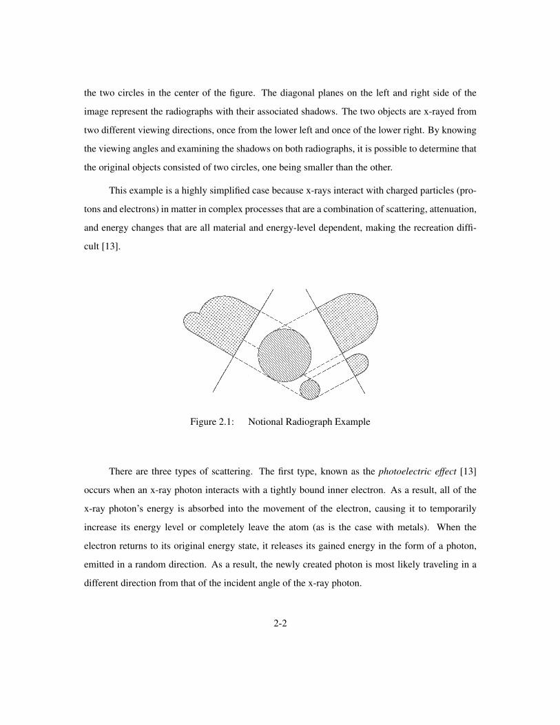
the two circles in the center of the figure. The diagonal planes on the left and right side of the

image represent the radiographs with their associated shadows. The two objects are x-rayed from

two different viewing directions, once from the lower left and once of the lower right. By knowing

the viewing angles and examining the shadows on both radiographs, it is possible to determine that

the original objects consisted of two circles, one being smaller than the other.

This example is a highly simplified case because x-rays interact with charged particles (pro-

tons and electrons) in matter in complex processes that are a combination of scattering, attenuation,

and energy changes that are all material and energy-level dependent, making the recreation diffi-

cult [13].

Figure 2.1: Notional Radiograph Example

There are three types of scattering. The first type, known as the photoelectric effect [13]

occurs when an x-ray photon interacts with a tightly bound inner electron. As a result, all of the

x-ray photon’s energy is absorbed into the movement of the electron, causing it to temporarily

increase its energy level or completely leave the atom (as is the case with metals). When the

electron returns to its original energy state, it releases its gained energy in the form of a photon,

emitted in a random direction. As a result, the newly created photon is most likely traveling in a

different direction from that of the incident angle of the x-ray photon.

2-2

The second type of scattering is referred to as Compton scattering [13]. In this case, the

x-ray photon interacts with a loosely bound outer electron and scatters off at an angle, while im-

parting some of its energy to the electron. Unlike the photoelectric effect, there is a strong angular

correlation between the incoming angle and the scattered angle. As a result, the reduced energy

photon is much more likely to be traveling in, or close to, its original path, parallel to the other

x-ray photons, than to bounce back in the direction from which it came from.

The final type of scattering, called pair production, occurs with photons with energies higher

than 1.022 mega-electron-volts (MeV). When high energy photons interact with an atom, they

temporarily produce an electron/positron pair that immediately destroy each other, producing two

photons of 0.511 MeV traveling in random but opposite directions. If the energy of the original

photon is higher than 1.022 MeV, the remaining energy would stay with the original photon [13].

As previously stated, these scattering processes are energy dependent. For medical imaging

as well as field deployed x-ray radiography devices, it is impractical to use x-rays that contain

mono-energetic (one energy level) photons because high intensities and high energies are difficult

to obtain from mono-energetic sources and are generally limited to laboratory applications. As

a result, polychromatic (multi-energetic) x-ray sources, which produce x-rays of varying photon

levels, are used because they are inexpensive and portable compared to monochromatic sources.

However, polychromatic sources only exacerbate the scattering issues addressed above because

x-ray photons of different energy levels scatter differently.

Another physical phenomenon, known as beam hardening, makes x-ray tomography difficult

when using a polychromatic source. It occurs because the linear attenuation coefficient (the amount

the x-ray’s intensity is reduced) is energy dependent. As a result, the beam’s spectral content (the

distribution of the x-ray beam’s energy) is different at the detector than at the source [34, 118].

2.1.2 Abel Inversion Tomography Techniques. Despite the difficulties identified in Sec-

tion 2.1.1, researchers at LANL believe that the Abel transform is useful for describing the tomo-

graphic measurement operator. In simplest terms, this operator is a linear transform P that maps

2-3

the object’s properties µ to the measured quantities d, obtained from the radiograph.

Pµ = d (2.1)

Ideally, (2.1) could be solved simply by taking the inverse P−1 of the linear transform. How-

ever, in x-ray tomography problems for cylindrically symmetric objects, such as in [14], detectors

measure photon intensity, and in order to determine the object’s density properties, intensity data

must be converted to the attenuation coefficient. This is accomplished through the use of the in-

verse Abel transform. In [14], the authors consider a one-dimensional recreation of the object from

a single radiograph with a single property description, µ(r), where r is the radial distance from the

center of the object. Neglecting the physical interactions of scattering, the continuous inverse Abel

transform for this case may be expressed as

µ(r) =− 1πr

ddr

Z∞

r

xd(x)√x2− r2

, (2.2)

where the attenuation coefficient µ is a line integral relative to the intensity d and x is the distance

on the radiograph.

However, direct inversion of the Abel transform is difficult because there is a singularity in

(2.2) at the lower limit of the integral. In order to address this difficulty, Asaki et al. [14] suggest

using the Abel transform,

d(x) = 2Z

∞

|x|

rµ(r)√r2− x2

dr, (2.3)

and not its inverse. The Abel transform is then discretized and formulated as a non-sparse matrix

P ∈ Rm×n with µ ∈ Rn and d ∈ Rm.

Other methods of performing indirect Abel inversion include fitting simple polynomial func-

tions (up to twelfth-order) to the data, or performing least-squares curve fitting methods and then

2-4

directly inverting [24]. In [49] the data is filtered using its Fourier Transform, while in [46] the

Abel transform is fit to the data by expanding the inverse with respect to a chosen basis.

Although the formulation of P as a matrix avoids the integral singularity in (2.2), discretiza-

tion produces poor results for several reasons [14]. First (2.3) is highly simplified and does not take

into account the physical interactions of scattering and polychromatic effects. Second, if m < n,

P is singular and thus cannot be inverted. Third, even when n ≈ m and P−1 exists, P becomes ill-

conditioned, meaning that small changes in d will lead to large deviations in µ, resulting in noise

amplification.

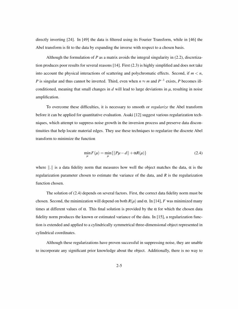
To overcome these difficulties, it is necessary to smooth or regularize the Abel transform

before it can be applied for quantitative evaluation. Asaki [12] suggest various regularization tech-

niques, which attempt to suppress noise growth in the inversion process and preserve data discon-

tinuities that help locate material edges. They use these techniques to regularize the discrete Abel

transform to minimize the function

minµ

F(µ) = minµ‖Pµ−d‖+αR(µ) (2.4)

where ‖.‖ is a data fidelity norm that measures how well the object matches the data, α is the

regularization parameter chosen to estimate the variance of the data, and R is the regularization

function chosen.

The solution of (2.4) depends on several factors. First, the correct data fidelity norm must be

chosen. Second, the minimization will depend on both R(µ) and α. In [14], F was minimized many

times at different values of α. This final solution is provided by the α for which the chosen data

fidelity norm produces the known or estimated variance of the data. In [15], a regularization func-

tion is extended and applied to a cylindrically symmetrical three-dimensional object represented in

cylindrical coordinates.

Although these regularizations have proven successful in suppressing noise, they are unable

to incorporate any significant prior knowledge about the object. Additionally, there is no way to

2-5

quantitatively determine the object’s material composition or even the number of layers in the ob-

ject. As a result of these difficulties, LANL researchers are turning to optimization methods that

avoid relying on regularization functions in order to find a quantitative solution to object recon-

struction that can take advantage of all prior knowledge of the object. In the next chapter, the

mixed variable pattern search algorithm is presented as a suitable approach to solving x-ray Abel

transform tomography object reconstruction problems.

2.2 Generalized Pattern Search (GPS) Methods

2.2.1 Linearly Constrained GPS. Generalized pattern search falls into the category of

direct search methods, which do not compute or approximate derivatives of the objective function

f . In a 1997 paper, Torczon [51] presents the class of GPS methods for solving unconstrained

minimization problems as a generalization of some other well-known methods, such as coordinate

search with fixed step sizes, evolutionary operation using factorial design [21], Hooke and Jeeves’

original direct search algorithm [33], and the multidirectional search algorithm [27]. In doing

so, she included a unifying convergence theory that does not require derivative information or a

sufficient decrease conditions.

At each iteration, the objective function f is evaluated at points lying on a mesh or lattice.

The mesh is defined as the set of all nonnegative integer combinations of vectors that form a positive

spanning set (see Definition 2.2.1). During each iteration, the mesh points lying adjacent to the

current iterate are evaluated. If improvement is found, the point is accepted and the mesh is either

retained or coarsened; otherwise, the mesh is refined by decreasing the mesh size. By limiting the

search to points on the mesh, Torczon [51] was able to show that if all iterates lie in a compact set

and the function f is continuously differentiable, then the mesh size becomes arbitrarily small. As a

result, there exists a subsequence of iterates that converges to a point x∗ that satisfies the first-order

necessary condition, ∇ f (x∗) = 0. More detail is given in Chapter III.

Lewis and Torczon [40] improved the efficiency of the algorithm in [51] by applying the

theory of a positive linear dependence [25]. In doing so, they were able to lower the worst case

2-6

cost of an iteration from 2n to n + 1 function evaluations while maintaining existing convergence

properties.

The following key definition and theorem come from [25]:

Definition 2.2.1 A finite set of vectors W = wiri=1 forms a positive spanning set for Rn, if every

v ∈ Rn can be expressed as v = ∑αiwi for some αi, i = 1,2, . . . ,r. The set of vectors W is said

to positively span Rn. The set W is said to be a positive basis for Rn if no proper subset of W

positively spans Rn.

Theorem 2.2.2 A set D positively spans Rn if and only if, for all nonzero v ∈Rn, vT d > 0 for some

d ∈ D.

Theorem 2.2.2 ensures that if ∇ f (x) exists at x and is nonzero, then (by choosing v = −∇ f (x))

there exists a d ∈ D, such that ∇ f (x)T d < 0. Thus, at least one d ∈ D is a direction of descent. In

pattern search, two very common choices for a positive basis include the columns of D = [I,−I]

and D = [I,−e], where I ∈ Rn×n is the identity matrix and e ∈ Rn is the vector of ones [40]. If

derivative information is available, Abramson, Audet, and Dennis [8] show how Theorem 2.2.2

can be applied to D = −1,0,1n to reduce the set of points to be evaluated to a singleton.

In subsequent papers, Lewis and Torczon extended GPS to bound [41] and linearly con-

strained [42] optimization problems of the form,

minx∈Rn

f (x)

s. t. l ≤ Ax ≤ u,(2.5)

where f : Rn → R, A ∈Qm×n, and l ≤ u.

They prove that if f is continuously differentiable and search directions include a set of

generators of the cone of feasible directions (with respect to all nearby constraints), then there

exists a subsequence of iterates that converges to a point x∗ satisfying the Karush-Kuhn-Tucker

(KKT) first-order necessary conditions for optimality.

2-7

The KKT conditions for linear equality constraints, originally published in 1952 by Kuhn

and Tucker [39], but also proved independently by Karush [35] nearly 15 years prior, are given in

Theorem 2.2.3 [47, 441] for the linearly constrained case. The first three conditions are referred to

as the first-order necessary conditions, while the last is the second-order necessary condition.

Theorem 2.2.3 If x∗ is a local minimizer of f over the set x : Ax ≥ b, then for some vector λ∗ of

Lagrange multipliers

• ∇ f (x∗) = AT λ∗, or equivalently, ZT ∇ f (x∗) = 0,

• λ∗ ≥ 0,

• λT∗ (Ax∗−b) = 0, and

• ZT ∇2 f (x∗)Z is positive semi-definite,

where Z is a matrix whose columns form a basis for the null-space of the active constraints at x∗.

Convergence behavior of GPS with respect to second-order stationary points is studied in [6] while

local convergence rates of GPS are studied in [28]. A thorough review of the more general class of

generating set search methods for linearly constrained nonlinear programming problems is given

in [38].

2.2.2 Mixed Variable GPS. In [16], Audet and Dennis extend GPS to problems that con-

tain both continuous and categorical variables with bound constraints on the continuous variables;

i.e., MVP problems of the form given in (1.1), in which A is the identity matrix. The algorithm they

present assumes the objective function f is continuously differentiable when the discrete variables

in Xd are fixed. As a result, their algorithm is a generalization of the basic GPS algorithm pre-

sented by Lewis and Torczon and reduces to such when the dimension nd = 0 (i.e. in the absence

of discrete variables).

Kokkolaras, Audet and Dennis [37] apply the MVP algorithm to the design of a thermal

insulation system, first considered by Hilal and Boom [32]. They demonstrate a 65% reduction in

2-8

the objective function value over previous results that applied other optimization methods. This

demonstration shows that the MVP algorithm is highly effective in solving a broad class of engi-

neering problems that were difficult to solve using earlier methods without incorporating engineer-

ing intuition into the problem. The Audet-Dennis GPS method for MVP problems was extended

further in [50] to problems with random noise in the objective function by adding a ranking and

selection scheme.

Two other methods for solving mixed variable problems, one derivative-based and one derivative-

free, were developed by Lucidi and Piccialli [44] and Lucidi, Piccialli, and Sciandrone [45], respec-

tively. In their more general framework, trial points are not restricted to lie on a mesh. This allows

any suitably chosen derivative-free method (in the case of [45]) to be used instead of pattern search

to guarantee convergence to a first-order stationary point. However, it requires a sufficient decrease

instead of the simple decrease requirement by pattern search.

2.2.3 GPS extensions. Motivated by the derivative-free nature of GPS, Audet and Den-

nis [17] introduced a new convergence analysis for linearly constrained problems, in which less

smoothness is required on the objective function f . They provide a hierarchy of results that depend

on the smoothness of f . Other extension of GPS include the use of a subprocedure that adap-

tively controls the precision of an approximating objective function [48] and the incorporation of a

user-provided scheme to generate points leading to potential objective function decrease [11].

GPS has also been extended to problems with nonlinear constraints. Lewis and Torczon

[43] adapt a bound constrained augmented Lagrangian method, first proposed in [23], as way to

apply a pattern search algorithm to optimization problems with general constraints and simple

bounds. They solve the bound constrained subproblem by replacing the stopping conditions pro-

posed in [23], which require derivatives, with stopping criteria based on mesh size. They demon-

strate convergence to a KKT point by linking the size of the pattern in the bound constrained pattern

search with the amount of local feasible descent.

2-9

Audet and Dennis [19] take a different approach to problems with nonlinear constraints

through the development of a filter method [19]. First developed by Fletcher and Leyffer in [29] as

a way to globalize sequential linear and quadratic programming, a filter algorithm accepts a step if

the objective function or a function measuring aggregate constraint violation is reduced. Audet and

Dennis’ GPS implementation of a filter method [19] only requires simple decrease in the objective

or constraint violation function, but does not guarantee convergence to a first-order KKT point.

The extension of [19] to mixed variable problems is presented in [4] which generalizes all of the

previous work of Audet and Dennis with convergence results that reduce to previously presented

results for the specific class of problems it covers. This approach is applied to a modified version

of the problem in [37], in which realistic nonlinear constraints have been added [5].

Motivated by the weaknesses in the convergence theory for the filter GPS algorithm, Audet

and Dennis generalize GPS for nonlinearly constrained problems by introducing a new direct search

method, known as mesh adaptive direct search (MADS) [18]. Unlike GPS, the MADS algorithm

does not limit the local exploration of the variable space to a finite number of directions. Instead,

MADS ensures an asymptotically dense set of directions. As the convergence theory demonstrates,

MADS iterates converge to a limit point satisfying both first-order [18] and second-order [7] nec-

essary or sufficient optimality conditions.

In the following chapters, a detailed description of the mixed variable GPS algorithm is

presented, along with its associated convergence theory. Implementation of the algorithm on the

LANL problem is discussed, followed by the numerical results and analysis of the algorithm on

several test cases of objects.

2-10

III. Methodology

This chapter describes the Audet-Dennis [16] class of pattern search algorithms for mixed vari-

able problems with linear constraints, including a summary of convergence results. Much of the

description comes from [4, 61-82] and [16]. The algorithm is then applied to the Los Alamos Na-

tional Laboratory (LANL) quantitative object reconstruction optimization problem and a detailed

discussion of the linear constraints and discrete neighbors is presented. Numerical results of this

application are discussed in Chapter IV.

As discussed in Chapter I, the LANL object reconstruction problem contains categorical

variables. recall, the vector of design variables x is partitioned into its continuous and categorical

components; namely, the continuous layer edge boundaries and the discrete number of types of

materials. Material types must be selected from a pre-defined list. The number of layers of materi-

als is also treated as a categorical variable, and a change in its value changes the linear constraints

and even the dimension of the problem. Because non-integer values of these variables do not make

physical sense, temporary relaxations can not be performed. This restriction results is not often

seen in other optimization problems.

3.1 GPS for Linearly Constrained MVP Problems

Pattern search is an iterative method that generates a sequence of feasible points with nonin-

creasing objective function values. At each iteration, the objective function is evaluated at a finite

number of points on a mesh in an attempt to find one that decreases the objective function value.

The mesh Mk at each iteration is a subset of the domain Ω ⊂ Rnc ×Znd.

3.1.1 Mesh Generation. At each iteration, the mesh can be formed as the direct product

of the union of a finite number of lattices in Rncwith the integer space Znd

, as follows. For each

combination i = 1,2, . . . , imax of values that the discrete variables may take on, a set of positive

3-1

spanning directions Di is formed by the product

Di = GiZi, (3.1)

where Gi ∈Rnc×ncis a nonsingular generating matrix and Zi ∈ Znc×|Di|. Then the mesh is the direct

product of Xd with a union of a finite number of lattices in Xc centered at the continuous part of

the current iterate:

Mk = Xd ×imax[i=1

xc +∆kDiz : z ∈ Z|Di|

+ . (3.2)

In this formulation the number of lattice points is finite and the minimum distance between

two distinct mesh points points is proportional to the mesh size parameter ∆k > 0. The mesh size

parameter controls the resolution (fineness or coarseness) of the mesh.

3.1.2 Local Optimality. To accommodate both continuous and categorical variables, the

GPS algorithm for bound [41] and linearly constrained [42] minimization was extended in [16]

and [4], respectively. In doing so, a concept of local optimality was introduced that accounts for

variations of both the continuous and categorical variables, but reduces to basic GPS in the absence

of categorical variables.

For problems consisting of only continuous variables, local optimality is well-defined: x∗ ∈

Rn is a local minimizer of f : Ω → R if there exists an ε > 0 such that f (x∗) ≤ f (v) for all v ∈

B(x∗,ε)∩Ω, where B(x∗,ε) is a ball of radius ε centered at x∗. For mixed variable problems,

this definition must be augmented to account for discrete variables. This is done by adding the

condition [4], f (x∗) ≤ f (y) for all y ∈ N (x∗), where N (x∗) is the set of discrete neighbors of x∗.

This is formally stated in Definition 3.1.1.

3-2

Definition 3.1.1 A point x∗ = (xc∗,x

d∗) ∈ X is said to be a local minimizer of f with respect to the

set of neighbors N (x)⊂ X if there exists an ε > 0 such that f (x)≤ f (v) for all v in the set

X ∩[

y∈N (x)

(B(yc,ε)× yd

). (3.3)

Definition 3.1.1 not only requires this additional condition, but it also requires that, if f (y) = f (x∗),

for all y ∈ N (x∗), then f (y) ≤ f (w) for all w ∈ B(y,ε)∩Ω. In order to guarantee convergence in

the mixed variable case, which is formally defined in Definition 3.1.2, a notion of continuity with

respect to the set of discrete neighbors is required for the set-valued function N : X → 2X , where

2X is the power set (or set of all possible subsets) of X. This is given in Definition 3.1.3 [4].

Definition 3.1.2 Let X ⊆ (Rnc ×Znd) be a mixed variable domain. A sequence xi ⊂ X is said

to converge to x ∈ X if, for every ε > 0, there exists a positive integer N such that xdi = xd and

‖xci − xc‖< ε for all i > N. The point x is said to be the limit point of the sequence xi.

Definition 3.1.3 The set-valued function N : X ⊆ (Rnc ×Znd)→ 2X is said to be continuous at x∈

X if, for every ε > 0, there exists δ > 0 such that, whenever u∈X satisfies ud = xd and ‖uc−xc‖< δ,

the following two conditions hold:

1. If y ∈ N (x), then there exists v ∈ N (u) satisfying vd = yd and ‖vc− yc‖< ε,

2. If v ∈ N (u), then there exists y ∈ N (x) satisfying yd = vd and ‖yc− vc‖< ε.

Note that each lattice in (3.2) is expressed as a translation from xck, instead of yc

k, for some yk ∈

N (xk). Additionally, the function N must also be constructed so that every discrete neighbor of

the current iterate lies on the current mesh Mk. Both of these conditions are necessary to ensure

convergence of the algorithm.

This concept of local optimality requires the user to decide how to define the neighborhood

function N . The algorithm will then produce a solution x, that, under certain conditions, will be

locally optimal with respect to its discrete neighbors N (x).

3-3

3.2 GPS for MVP with Linear Constraints Algorithm

With a newly constructed mesh and local optimality for the mixed variable case defined, it

is possible to discuss the algorithm for mixed variable problems with linear constraints given by

Abramson [4]. The goal of each iteration of the algorithm is to find a point on the current mesh

whose objective value is less than that of the current incumbent. In order to find such a point, the

mesh is explored in three phases.

3.2.1 SEARCH Step. The first phase, the SEARCH, is simply a search of a finite number

of trial points Sk on the mesh Mk where the objective function is evaluated at each point in Sk.

This phase is typically more global in nature, and it is free of any any other rules imposed by

the algorithm and can be performed anywhere on the mesh. The flexibility in this step allows

any strategy (including none) to be specified by the user. One choice is a meta-heuristic such

as simulated annealing [36], tabu search [30, 31], or genetic algorithms [26]. Additionally, if f

is computationally expensive to evaluate, one common approach is to construct and optimize an

inexpensive surrogate function [20] at each SEARCH step. In fact, any other ad/hoc search could be

used to improve upon the incumbent.

3.2.2 POLL Step. The second phase in the algorithm is the POLL step. Polling occurs

whenever the SEARCH step is unsuccessful in finding a point on the current mesh that decreased

the objective function value. Polling is done in two steps:

1. polling with respect to the continuous variables at xk

2. polling on the current set of discrete neighbors N (xk).

The first step is identical to that of pattern search algorithms for continuous variables only [17,

51, 41, 42, 40]. Polling with respect to continuous variables requires use of positive spanning sets

in Rnc. Let Di

k ⊆ Di denote the set of poll directions corresponding to the i-th set of discrete vari-

ables for each iteration k. The poll set Pk(xk), centered at xk, is the set of neighboring mesh points

3-4

in the directions Dik, while holding the discrete variables fixed; i.e.,

Pk(xk) = xk∪xk +∆k(d,0) ∈ X : d ∈ Dik ⊂ Mk ⊂ X . (3.4)

The notation (d,0) accounts for the partitioning into continuous and discrete variables, where 0

represents no change in the discrete variables. Therefore, xck +∆k(d,0) = (xc

k +∆kd,xdk ). If polling

with respect to the continuous variables fails to find a point in Pk(xk) that lowers the objective

function value, polling on the current set of discrete neighbors N (xk) is performed. The objective

function f is evaluated at each of the points in Pk(xk) until a lower objective function is found or

until all points have been evaluated.

3.2.3 EXTENDED POLL Step. In the event that both the poll set and set of discrete

neighbors fails to find improvement in the objective function value, the algorithm performs the

third step, called EXTENDED POLL, before declaring the iteration unsuccessful [16]. In this step,

additional polling is performed around each discrete neighbor point y ∈ N (xk), whose objective

function value was only a small amount greater than that of the incumbent. This is done because

y ∈ N (xk) is a promising point and a poll around y may produce a better objective function value

than the incumbent. The EXTENDED POLL step is performed whenever f (yk) < f (xk)+ξk, where

the extended poll trigger ξk satisfies ξk ≥ ξ for a fixed ξ > 0. The values for ξk are often set as

a percentage of the objective function value at the current iterate [4]. Large ξ values should yield

a better local minimizer, but would generate more EXTENDED POLLs, resulting in an increase of

function evaluations.

For each iteration k, the set of extended poll points for a discrete neighbor y ∈ Nk, denoted

εy, is evaluated and forms the extended poll set given by

Nk =[

y∈N ξ

k

ε(y) (3.5)

3-5

where N ξ

k = y ∈ N (xk) : f (xk)≤ f (y)≤ f (xk)+ξk. Polling then begins around the continuous

neighbors of yk in a sequence y jk

Jkj=1 and continues until either all continuous neighbors have been

evaluated or until a point is found that decreases the objective function value. The endpoint of the

EXTENDED POLL step, is denoted as zk.

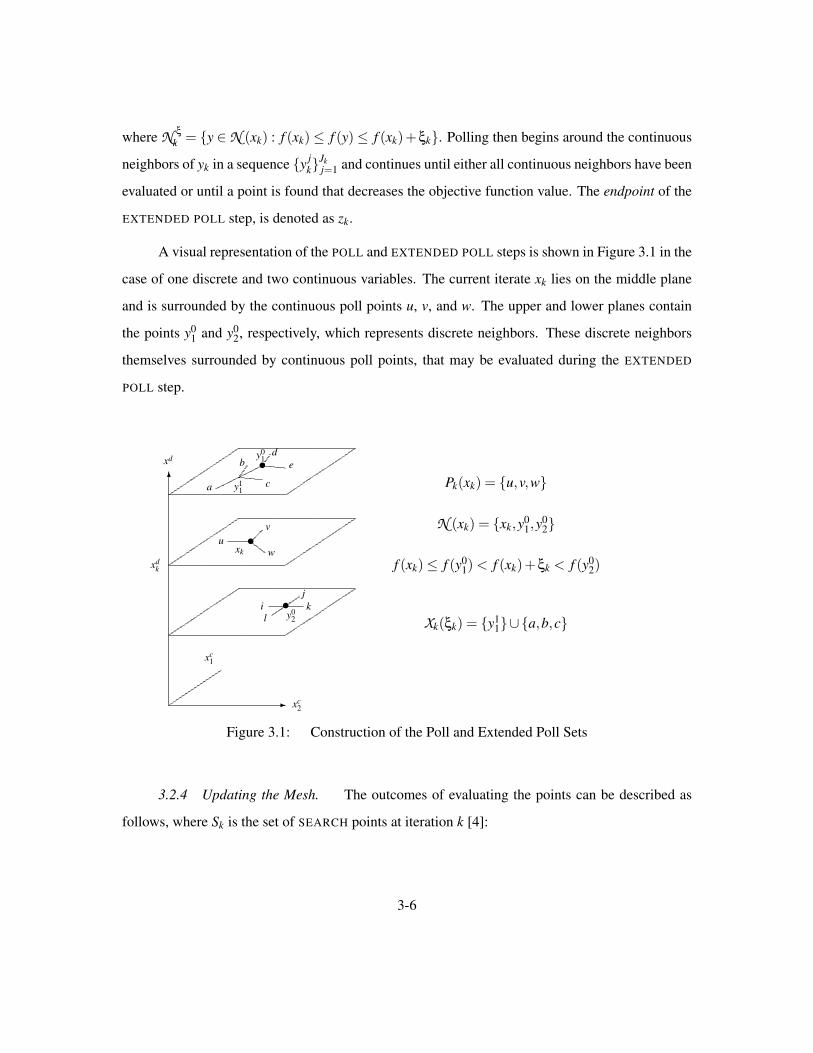
A visual representation of the POLL and EXTENDED POLL steps is shown in Figure 3.1 in the

case of one discrete and two continuous variables. The current iterate xk lies on the middle plane

and is surrounded by the continuous poll points u, v, and w. The upper and lower planes contain

the points y01 and y0

2, respectively, which represents discrete neighbors. These discrete neighbors

themselves surrounded by continuous poll points, that may be evaluated during the EXTENDED

POLL step.

-

6

xc1

xc2

xd

xdk

•

•

•

y01

xk

y02

y11

de

a

b

c

uv

w

ijk

l

Pk(xk) = u,v,w

N (xk) = xk,y01,y

02

f (xk)≤ f (y01) < f (xk)+ξk < f (y0

2)

Xk(ξk) = y11∪a,b,c

Figure 3.1: Construction of the Poll and Extended Poll Sets

3.2.4 Updating the Mesh. The outcomes of evaluating the points can be described as

follows, where Sk is the set of SEARCH points at iteration k [4]:

3-6

Definition 3.2.1 If f (y) < f (xk) for some y ∈ Sk ∪Pk(xk)∪N (xk)∪X (ξk), then y is said to be an

improved mesh point.

Definition 3.2.2 If f (xk) ≤ f (y) for all y ∈ Pk(xk)∪N (xk)∪Xk(ξk), then xk is said to be a mesh

local optimizer.

If the SEARCH, POLL, or EXTENDED POLL step is successful in finding an improved mesh point, it

becomes the new incumbent xk+1, in which case, the mesh is either retained or coarsened according

to the following rule [9],

∆k+1 = τm+

k ∆k, (3.6)

where m+k ∈ 0,1, . . . ,mmax for some mmax ∈ Z+ and τ > 1 is rational and fixed over all iterations.

This formulation allows the mesh to be retained at the same size when m+k = 0. Mesh coarsening

does not affect theoretical convergence properties. It can slow or speed convergence, but it can also

cause the algorithm to skip over a local minimum and find a better one [9] .

If the SEARCH, POLL, and EXTENDED POLL steps are unsuccessful, then the incumbent is a

mesh local optimizer and is retained (i.e. xk+1 = xk) and the mesh must be refined by the rule [9],

∆k+1 = τm−

k ∆k, (3.7)

where m−k ∈ mmin,mmin+1, . . . ,−1. The GPS algorithm is for linearly constrained MVP problems

is fully described in Figure 3.2.

3.2.5 Treating Linear Constraints. To treat linear constraints, infeasible points are sim-

ply ignored and not evaluated by the objective function. To guarantee convergence, the only ad-

ditional requirement is that polling directions must be chosen that conform to the geometry of

the linear constraint boundaries and that these directions are used an infinite number of times [4].

Definition 3.2.3 [17] abstracts the idea of conforming directions.

3-7

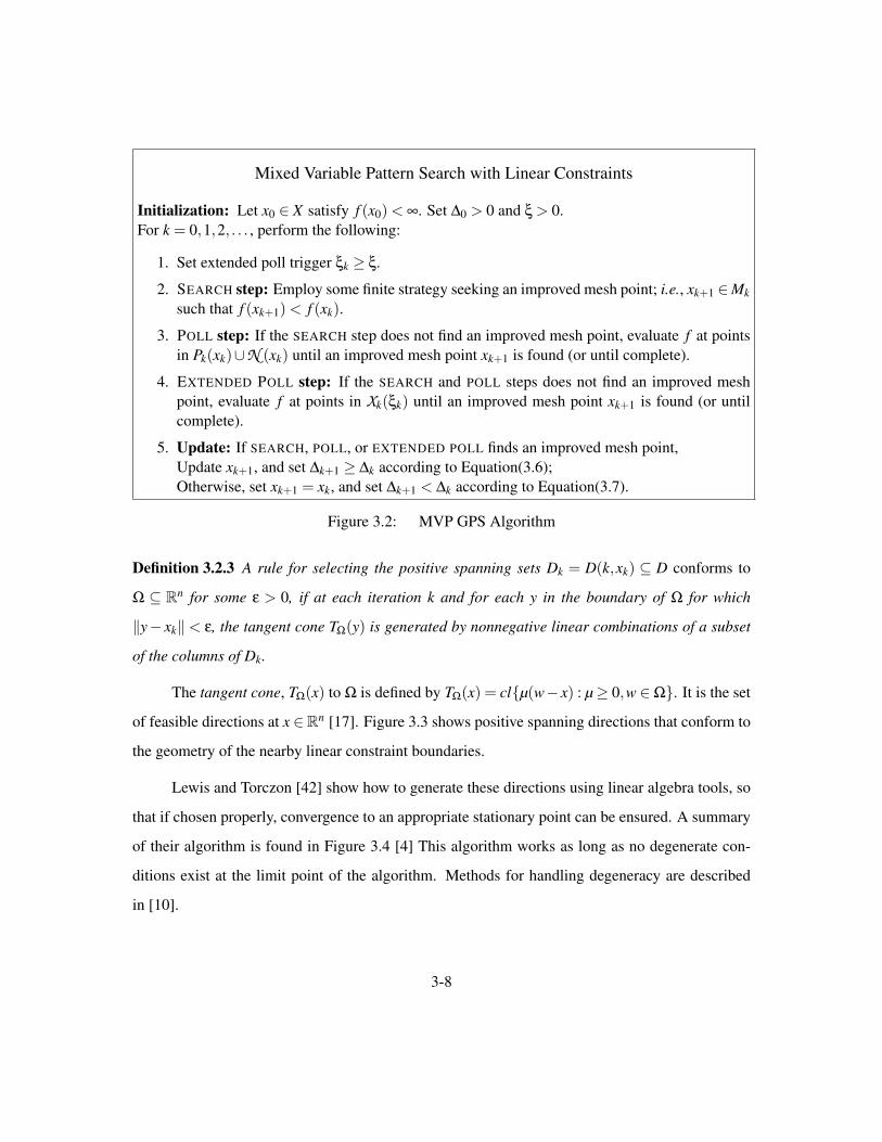
Mixed Variable Pattern Search with Linear Constraints

Initialization: Let x0 ∈ X satisfy f (x0) < ∞. Set ∆0 > 0 and ξ > 0.For k = 0,1,2, . . . , perform the following:

1. Set extended poll trigger ξk ≥ ξ.

2. SEARCH step: Employ some finite strategy seeking an improved mesh point; i.e., xk+1 ∈Mksuch that f (xk+1) < f (xk).

3. POLL step: If the SEARCH step does not find an improved mesh point, evaluate f at pointsin Pk(xk)∪N (xk) until an improved mesh point xk+1 is found (or until complete).

4. EXTENDED POLL step: If the SEARCH and POLL steps does not find an improved meshpoint, evaluate f at points in Xk(ξk) until an improved mesh point xk+1 is found (or untilcomplete).

5. Update: If SEARCH, POLL, or EXTENDED POLL finds an improved mesh point,Update xk+1, and set ∆k+1 ≥ ∆k according to Equation(3.6);Otherwise, set xk+1 = xk, and set ∆k+1 < ∆k according to Equation(3.7).

Figure 3.2: MVP GPS Algorithm

Definition 3.2.3 A rule for selecting the positive spanning sets Dk = D(k,xk) ⊆ D conforms to

Ω ⊆ Rn for some ε > 0, if at each iteration k and for each y in the boundary of Ω for which

‖y− xk‖ < ε, the tangent cone TΩ(y) is generated by nonnegative linear combinations of a subset

of the columns of Dk.

The tangent cone, TΩ(x) to Ω is defined by TΩ(x) = clµ(w−x) : µ≥ 0,w ∈Ω. It is the set

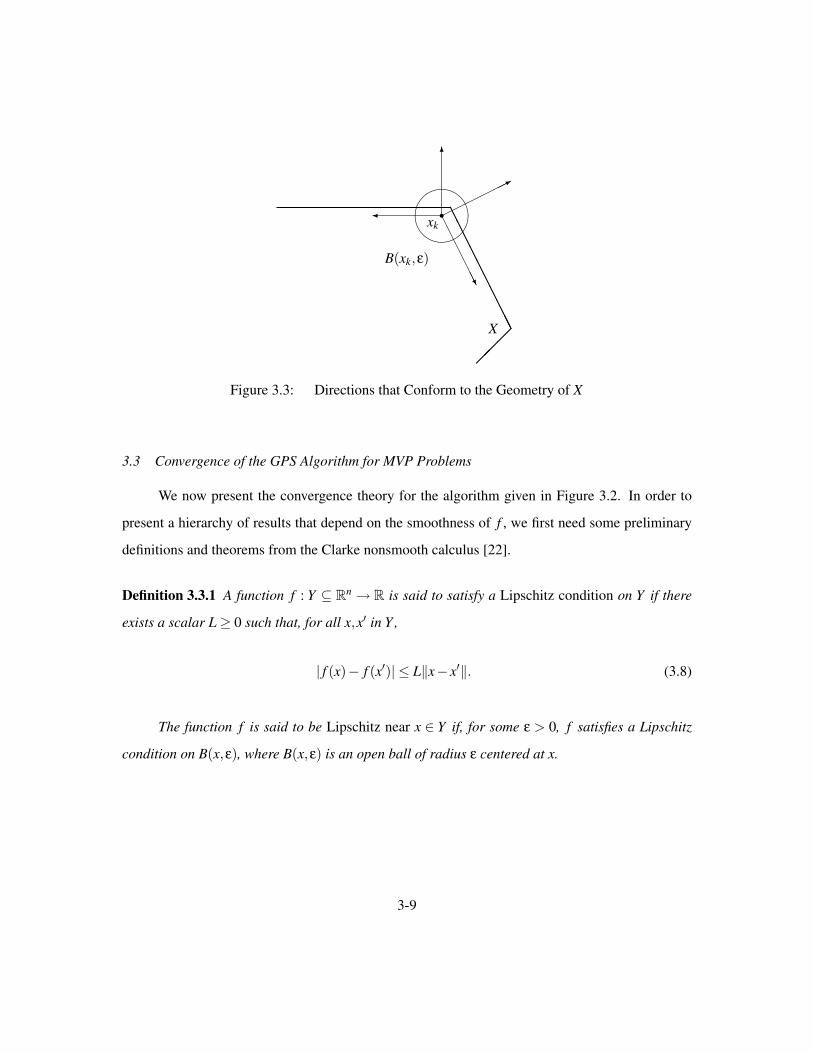
of feasible directions at x ∈Rn [17]. Figure 3.3 shows positive spanning directions that conform to

the geometry of the nearby linear constraint boundaries.

Lewis and Torczon [42] show how to generate these directions using linear algebra tools, so

that if chosen properly, convergence to an appropriate stationary point can be ensured. A summary

of their algorithm is found in Figure 3.4 [4] This algorithm works as long as no degenerate con-

ditions exist at the limit point of the algorithm. Methods for handling degeneracy are described

in [10].

3-8

AAAAAAAAAA

X

rxk

AAAAAAU

6

*

&%'$

B(xk,ε)

Figure 3.3: Directions that Conform to the Geometry of X

3.3 Convergence of the GPS Algorithm for MVP Problems

We now present the convergence theory for the algorithm given in Figure 3.2. In order to

present a hierarchy of results that depend on the smoothness of f , we first need some preliminary

definitions and theorems from the Clarke nonsmooth calculus [22].

Definition 3.3.1 A function f : Y ⊆ Rn → R is said to satisfy a Lipschitz condition on Y if there

exists a scalar L ≥ 0 such that, for all x,x′ in Y ,

| f (x)− f (x′)| ≤ L‖x− x′‖. (3.8)

The function f is said to be Lipschitz near x ∈ Y if, for some ε > 0, f satisfies a Lipschitz

condition on B(x,ε), where B(x,ε) is an open ball of radius ε centered at x.

3-9

Algorithm for Computing Conforming Directions Dk

• Set εk ≥ ε > 0. Assume the current iterate xk satisfies `≤ Axk ≤ u.• While εk ≥ ε, do the following:

1. Let I`(xk,εk) = i : Ax− `≤ εk2. Let Iu(xk,εk) = i : u−Ax ≤ εk3. Set V denote the matrix whose columns are formed by all the members of the

set −ai : i ∈ I`(xk,εk)∪ai : i ∈ Iu(xk,εk), where aTi denotes the i-th row of

A.

4. If V does not have full column rank, then reduce εk just until |I`(xk,εk)|+|Iu(xk,εk)| is decreased, and return to step 1.

• Set B = V (V TV )V−1 and N = I−V (V TV )V−1V T .• Set Dk = [N,−N, B,−B].

Figure 3.4: Algorithm for Generating Conforming Directions

Definition 3.3.2 (Clarke) Let f : Rn → R be Lipschitz near a given point x. The generalized

directional derivative of f at x in the direction v is given by

f (x;v) := limsupy→x,t↓0

f (y+ tv)− f (y)t

, (3.9)

where t is a positive scalar.

Definition 3.3.3 The function f : Rn → R is said to be strictly differentiable at x if, for all v ∈ Rn,

limy→x,t↓0

f (y+ tv)− f (y)t

= ∇ f (x)T v. (3.10)

3-10

Additionally, to ensure convergence, the following assumptions are made.

A1: All iterates xk produced by the algorithm lie in a compact set.

A2: For each fixed set of discrete variable values xd , the corresponding set of directions Di = GiZi,

includes tangent cone generators for every point in Xc(xd).

A3: The rule for selecting directions Dk conforms to Xc for some ε > 0.

A4: The discrete neighbors always lie on the mesh; i.e., N (xk)⊂Mk for all k

3.3.1 Mesh Size Behavior and Limit Points. Torczon [51] shows that, under Assumption

A1 and the additional assumptions of a continuously differentiable objective function, the mesh size

becomes arbitrarily small and the mesh size parameters are bounded above by a positive constant

that is independent of the iteration. This idea is formally presented in Theorem 3.3.4 and reproved

in [16] and [4] for MVP problems.

Theorem 3.3.4 The mesh size parameters satisfy liminfk→+∞

∆k = 0.

The following definitions, adapted from Audet and Dennis [17] are needed in order redefine

the concept of a limit direction for mixed variable spaces.

Definition 3.3.5 A subsequence of GPS mesh local optimizers xkk∈K (for some subset of indices

K) is said to be a refining subsequence if ∆kk∈K converges to zero.

Definition 3.3.6 Let vkk∈K be either a refining subsequence or a corresponding subsequence of

extended poll endpoints, and let v be a limit point of the subsequence. A direction d ∈ D is said to

be a refining direction of v if wk = vk +∆k(d,0) ∈ X and f (vk)≤ f (wk) for infinitely many k ∈ K.

Additionally, Theorem 3.3.7 [16] establishes the existence of limit points of interest. This demon-

strates the existence of a limit point of subsequences of interest. Finally, they establish the local

optimality conditions the limit point x satisfies with respect to the discrete variables.

3-11

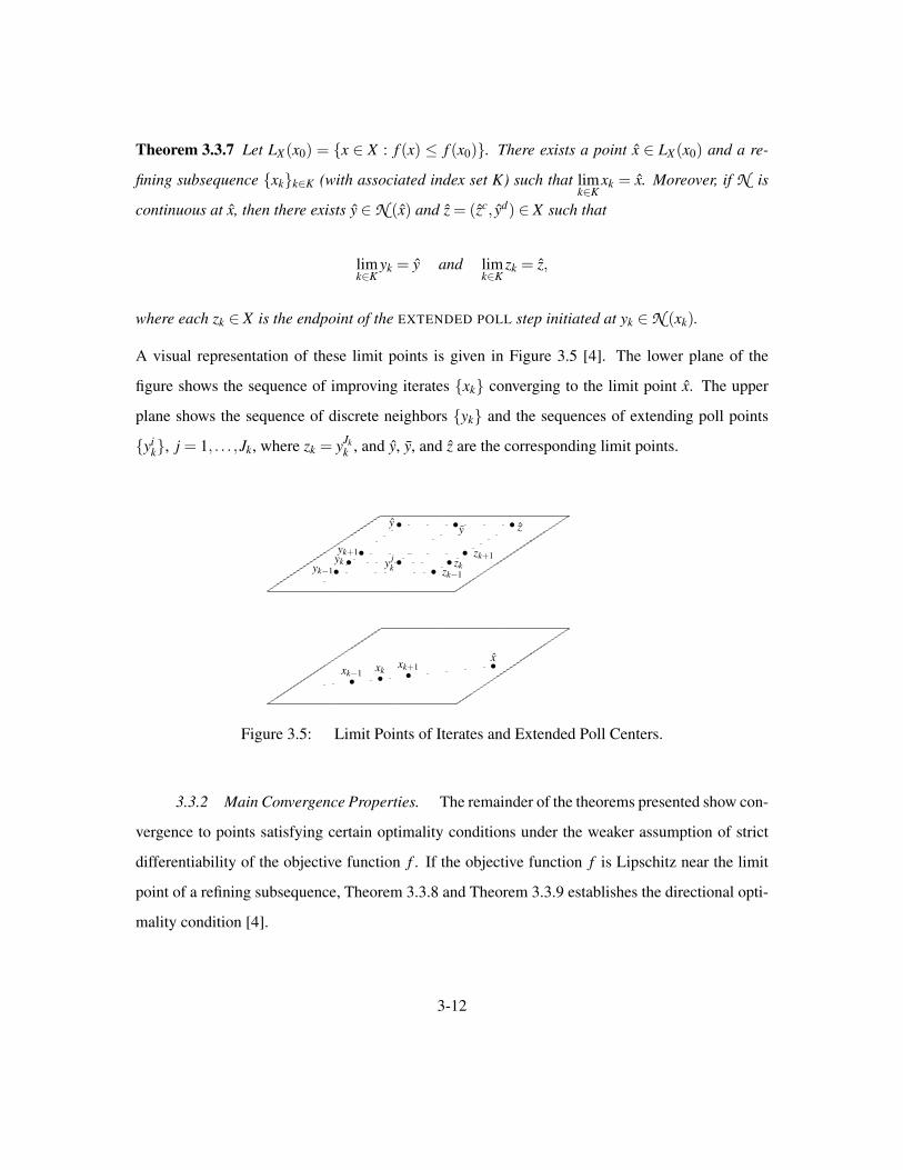
Theorem 3.3.7 Let LX(x0) = x ∈ X : f (x) ≤ f (x0). There exists a point x ∈ LX(x0) and a re-

fining subsequence xkk∈K (with associated index set K) such that limk∈K

xk = x. Moreover, if N is

continuous at x, then there exists y ∈ N (x) and z = (zc, yd) ∈ X such that

limk∈K

yk = y and limk∈K

zk = z,

where each zk ∈ X is the endpoint of the EXTENDED POLL step initiated at yk ∈ N (xk).

A visual representation of these limit points is given in Figure 3.5 [4]. The lower plane of the

figure shows the sequence of improving iterates xk converging to the limit point x. The upper

plane shows the sequence of discrete neighbors yk and the sequences of extending poll points

yik, j = 1, . . . ,Jk, where zk = yJk

k , and y, y, and z are the corresponding limit points.

• • ••xk−1 xk

xk+1x

•••

•

yk−1ykyk+1

y

••

•

•

zk−1zk

zk+1

z

•y jk

•y

Figure 3.5: Limit Points of Iterates and Extended Poll Centers.

3.3.2 Main Convergence Properties. The remainder of the theorems presented show con-

vergence to points satisfying certain optimality conditions under the weaker assumption of strict

differentiability of the objective function f . If the objective function f is Lipschitz near the limit

point of a refining subsequence, Theorem 3.3.8 and Theorem 3.3.9 establishes the directional opti-

mality condition [4].

3-12

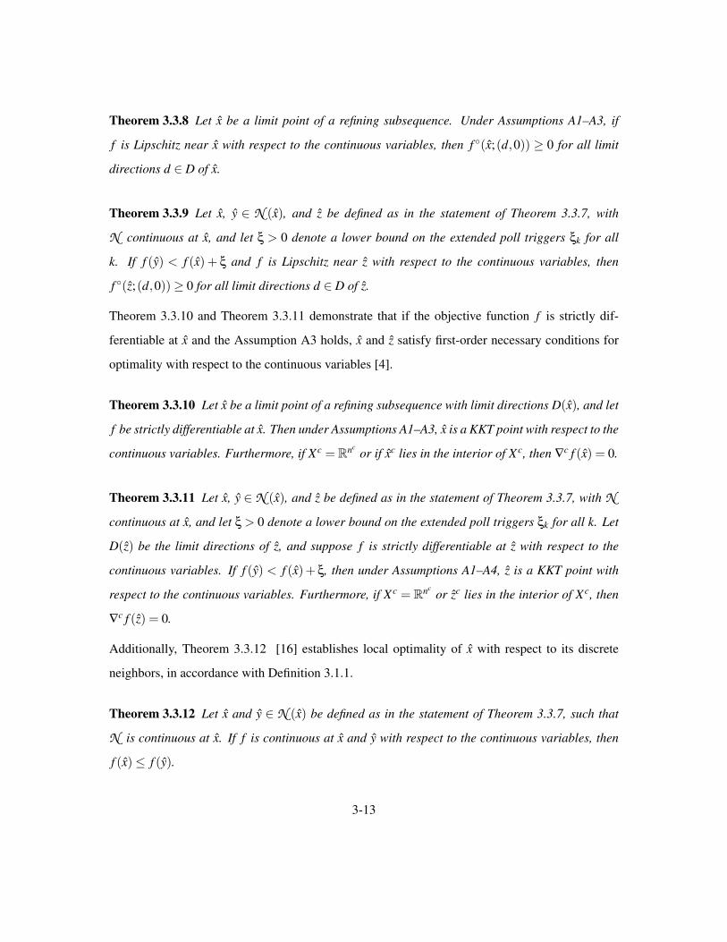
Theorem 3.3.8 Let x be a limit point of a refining subsequence. Under Assumptions A1–A3, if

f is Lipschitz near x with respect to the continuous variables, then f (x;(d,0)) ≥ 0 for all limit

directions d ∈ D of x.

Theorem 3.3.9 Let x, y ∈ N (x), and z be defined as in the statement of Theorem 3.3.7, with

N continuous at x, and let ξ > 0 denote a lower bound on the extended poll triggers ξk for all

k. If f (y) < f (x) + ξ and f is Lipschitz near z with respect to the continuous variables, then

f (z;(d,0))≥ 0 for all limit directions d ∈ D of z.

Theorem 3.3.10 and Theorem 3.3.11 demonstrate that if the objective function f is strictly dif-

ferentiable at x and the Assumption A3 holds, x and z satisfy first-order necessary conditions for

optimality with respect to the continuous variables [4].

Theorem 3.3.10 Let x be a limit point of a refining subsequence with limit directions D(x), and let

f be strictly differentiable at x. Then under Assumptions A1–A3, x is a KKT point with respect to the

continuous variables. Furthermore, if Xc = Rncor if xc lies in the interior of Xc, then ∇c f (x) = 0.

Theorem 3.3.11 Let x, y ∈ N (x), and z be defined as in the statement of Theorem 3.3.7, with N

continuous at x, and let ξ > 0 denote a lower bound on the extended poll triggers ξk for all k. Let

D(z) be the limit directions of z, and suppose f is strictly differentiable at z with respect to the

continuous variables. If f (y) < f (x)+ ξ, then under Assumptions A1–A4, z is a KKT point with

respect to the continuous variables. Furthermore, if Xc = Rncor zc lies in the interior of Xc, then

∇c f (z) = 0.

Additionally, Theorem 3.3.12 [16] establishes local optimality of x with respect to its discrete

neighbors, in accordance with Definition 3.1.1.

Theorem 3.3.12 Let x and y ∈ N (x) be defined as in the statement of Theorem 3.3.7, such that

N is continuous at x. If f is continuous at x and y with respect to the continuous variables, then

f (x)≤ f (y).

3-13

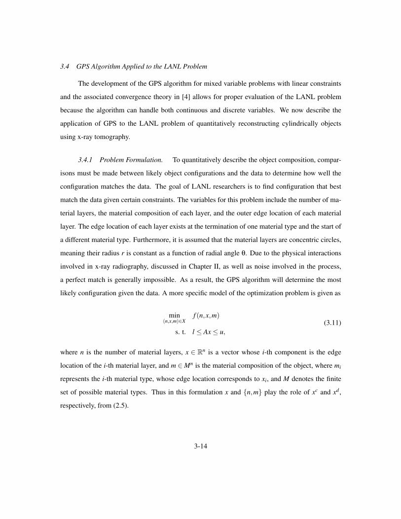
3.4 GPS Algorithm Applied to the LANL Problem

The development of the GPS algorithm for mixed variable problems with linear constraints

and the associated convergence theory in [4] allows for proper evaluation of the LANL problem

because the algorithm can handle both continuous and discrete variables. We now describe the

application of GPS to the LANL problem of quantitatively reconstructing cylindrically objects

using x-ray tomography.

3.4.1 Problem Formulation. To quantitatively describe the object composition, compar-

isons must be made between likely object configurations and the data to determine how well the

configuration matches the data. The goal of LANL researchers is to find configuration that best

match the data given certain constraints. The variables for this problem include the number of ma-

terial layers, the material composition of each layer, and the outer edge location of each material

layer. The edge location of each layer exists at the termination of one material type and the start of

a different material type. Furthermore, it is assumed that the material layers are concentric circles,

meaning their radius r is constant as a function of radial angle θ. Due to the physical interactions

involved in x-ray radiography, discussed in Chapter II, as well as noise involved in the process,

a perfect match is generally impossible. As a result, the GPS algorithm will determine the most

likely configuration given the data. A more specific model of the optimization problem is given as

min(n,x,m)∈X

f (n,x,m)

s. t. l ≤ Ax ≤ u,

(3.11)

where n is the number of material layers, x ∈ Rn is a vector whose i-th component is the edge

location of the i-th material layer, and m ∈ Mn is the material composition of the object, where mi

represents the i-th material type, whose edge location corresponds to xi, and M denotes the finite

set of possible material types. Thus in this formulation x and n,m play the role of xc and xd ,

respectively, from (2.5).

3-14

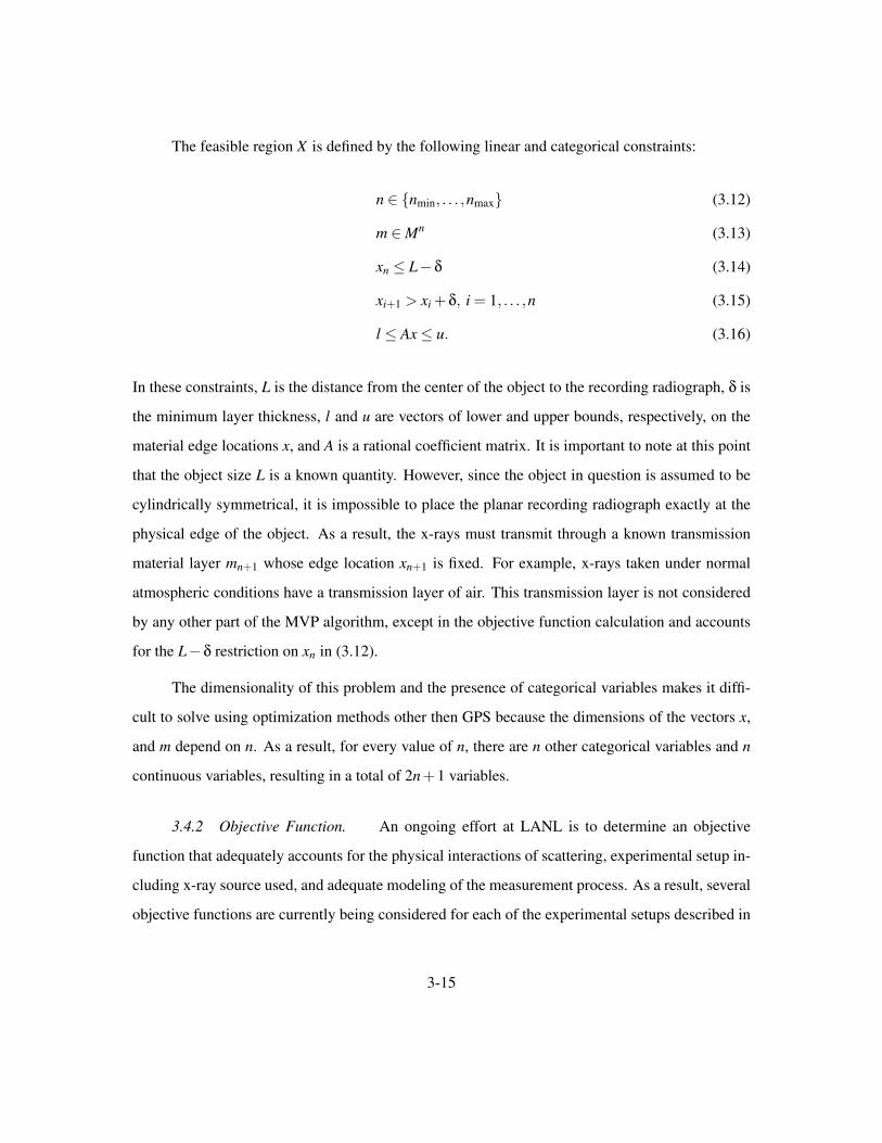
The feasible region X is defined by the following linear and categorical constraints:

n ∈ nmin, . . . ,nmax (3.12)

m ∈ Mn (3.13)

xn ≤ L−δ (3.14)

xi+1 > xi +δ, i = 1, . . . ,n (3.15)

l ≤ Ax ≤ u. (3.16)

In these constraints, L is the distance from the center of the object to the recording radiograph, δ is

the minimum layer thickness, l and u are vectors of lower and upper bounds, respectively, on the

material edge locations x, and A is a rational coefficient matrix. It is important to note at this point

that the object size L is a known quantity. However, since the object in question is assumed to be

cylindrically symmetrical, it is impossible to place the planar recording radiograph exactly at the

physical edge of the object. As a result, the x-rays must transmit through a known transmission

material layer mn+1 whose edge location xn+1 is fixed. For example, x-rays taken under normal

atmospheric conditions have a transmission layer of air. This transmission layer is not considered

by any other part of the MVP algorithm, except in the objective function calculation and accounts

for the L−δ restriction on xn in (3.12).

The dimensionality of this problem and the presence of categorical variables makes it diffi-

cult to solve using optimization methods other then GPS because the dimensions of the vectors x,

and m depend on n. As a result, for every value of n, there are n other categorical variables and n

continuous variables, resulting in a total of 2n+1 variables.

3.4.2 Objective Function. An ongoing effort at LANL is to determine an objective

function that adequately accounts for the physical interactions of scattering, experimental setup in-

cluding x-ray source used, and adequate modeling of the measurement process. As a result, several

objective functions are currently being considered for each of the experimental setups described in

3-15

Chapter IV; however, all of the objective functions are currently of the form,

f (u) =‖Pu−d‖2√

Lw

, (3.17)

where the operator P is the discretized Abel projection matrix, w is the radiograph pixel width

(square pixels are assumed), u ∈ R Lw is a pixelized version of the object and is a function of the

edge locations x and material types m, and d ∈ R Lw is the data from the radiograph. The P operator

is scaled to the unit radiograph data pixel width w. Therefore, P is an Lw ×

Lw matrix that reconstructs

the object from u at the maximum resolution that can be ascertained from the radiograph data and is

a linear geometric projection of a circularly discretized object. Regardless of the form the objective

function takes, the goal is to find the most likely recreation of the object’s composition that matches

the data from radiograph.

3.4.3 Linear Constraints. Although the constraints from (3.11) only apply to the contin-

uous variables, the material layer edge locations x, they are also functions of the number of material

layers n, a categorical variable. As a result, changes in the categorical variables may necessitate

a change in the continuous variables. The linear constraints on material edge layer locations are

specified in each problem by the user through a fixed minimum thickness δ of each material layer,

as well as the maximum edge location of the outermost material layer L−δ.

In order to obey the linear constraints, it is useful to compare the edge locations of adjacent

layers. The thickness of material layer mi is computed simply as the difference in edge locations;

namely xi− xi−1, i = 1,2, . . . ,n, where x0 = 0 and xn ≤ L− δ. Additionally, the lower and upper

bound on the innermost and outermost materials layer must be be taken into account. This results in

the formation of a rational coefficient matrix A ∈ R(n+1)×n with ones on the diagonal and negative

ones on the sub-diagonal, and with the n + 1 row containing all zeroes except for a one in the last

3-16

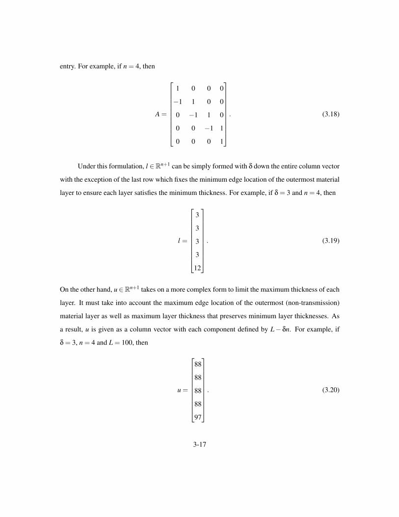
entry. For example, if n = 4, then

A =

1 0 0 0

−1 1 0 0

0 −1 1 0

0 0 −1 1

0 0 0 1

. (3.18)

Under this formulation, l ∈Rn+1 can be simply formed with δ down the entire column vector

with the exception of the last row which fixes the minimum edge location of the outermost material

layer to ensure each layer satisfies the minimum thickness. For example, if δ = 3 and n = 4, then

l =

3

3

3

3

12

. (3.19)

On the other hand, u∈Rn+1 takes on a more complex form to limit the maximum thickness of each

layer. It must take into account the maximum edge location of the outermost (non-transmission)

material layer as well as maximum layer thickness that preserves minimum layer thicknesses. As

a result, u is given as a column vector with each component defined by L− δn. For example, if

δ = 3, n = 4 and L = 100, then

u =

88

88

88

88

97

. (3.20)

3-17

3.4.4 Discrete Neighbors. Recall from Definition 3.1.1 that a set of discrete neighbors

must be defined by the user. Thus, when a solution to a MVP problem is found, it is always with

respect to this set of discrete neighbors. A general neighborhood structure where every set of

discrete variable is a neighbor of all other sets of discrete neighbors may result in a more global

solution, but at a very high computational cost [4]. However, underlying knowledge of the physical

processes involved in the problem allows restriction of the size of the set of neighbors that must

be examined at each iteration. As a result, there exists the possibility of significant savings in

computational cost and time, but may result in a more localized optimizer with a higher objective

function value.

The neighborhood structure of the discrete neighbors is perhaps the most interesting aspect

of the MVP GPS application to the LANL problem. It takes into account inherent properties of

Abel transform x-ray tomography, as well as known properties of the material types. Three types

of neighbors were permitted:

1. Swapping any layer with a material of a different type

2. The deletion of any single material layer

3. The addition of a single material layer between two existing layers

These neighbors were chosen to limit the size of the set of discrete neighbors and to ensure that

each neighbor was a mesh point. Otherwise, if the set of neighbors is not restricted in this way,

then it would containnmax

∑n=1

mn points at a given point, which would need to be evaluated during every

unsuccessful iteration. This number grows very fast, even for modest values of m and n.

In order to take advantage of underlying knowledge of the physical processes involved in

the problem, a user-defined adjacency matrix was utilized. The matrix, is square and binary, and

each row or column represents a material type. A value of 1 in the (i, j)th element means that

material i is adjacent to material j. It is likely that a user would desire an adjacency matrix that

is fully connected. A fully connected matrix implies that any material can be reached from any

other material either directly or through other materials [1]. Adjacent materials may be thought of

3-18

as materials that may be confused for one another in the current object configuration. To prevent

redundant neighbors, a material is not considered adjacent to itself. For example, lead and iron

affect the scattering and attenuation of x-ray photons as they pass through these materials in similar

manners. Thus, it is easy to confuse lead and iron when analyzing the results of a radiograph. As

a result, these materials may be considered adjacent; however, since lead is not easily confused

with air, they are not considered adjacent to each other. Information in the adjacency matrix was

utilized in each of the three types of neighbors examined in order to limit the size of the set of

discrete neighbors.

In addition to an adjacency matrix, information about the process of Abel transform x-ray

tomography was used to determine the order in which the neighbors that were evaluated. Changes

to the outside material layers affect more of the data than the inside layers. As a result, neighbors

with changes to the outside material layers were always evaluated before those with changes to

internal material layers because more change in the objective function is expected. For each type

of neighbor examined, there are unique considerations, which are due to the adjacency matrix, the

presence of the transmission material, and the minimum and maximum number layers permitted.

As such, each type of neighbor considered will be discussed in detail.

A swap of a material involves replacing one material in a layer with another material from

the material library M while layer thicknesses remain fixed. It is the simplest of neighbor types and

has the least restrictions. The only restriction on the swap is that the new material must be adjacent

to that of the old material, as defined by the adjacency matrix. Additionally, if the outermost layer

mn is to be swapped, the material of the transmission layer mn+1 cannot be considered.

The deletion of a material layer is slightly more complex than a simple material swap. Any

layer mi maybe considered for deletion if either the interior or exterior material layer, mi−1 or mi+1,

respectively, is adjacent to the material layer being considered, and provided that the current num-

ber of material layers n is greater than the minimum number of material layers nmin. However, if

outermost material layer mn is considered and the interior material layer mn−1 is of the same ma-

terial type as the transmission layer, both the outermost material layer mn and the interior material

3-19

layer mn−1 will be deleted. In the case of deletion of material layer mi, the corresponding edge

location xi will also be deleted. The material layer exterior mi+1 simply absorbs the thickness of

the deleted material layer. Again, material layer deletion is considered first at material layer mn and

works interior to material layer m1.

The addition of a material layer is the most complex type of neighbor because it requires the

addition of an edge location. All materials in the library M are considered for addition exterior

to material layer mi, as long as the material being considered is adjacent to either material layer

mi or mi+1, and provided that the current number of material layers n is less than the maximum

number of material layers mmax. The new edge location is simply located halfway between the edge

locations of the interior and exterior layers, xi and xi+1, respectively. If the material layer being

added is exterior to the outermost layer mn, the transmission material layer mn+1 is considered for

adjacency, and L is considered for the exterior layer location.

Although specific values were used in this section as demonstrative examples to further the

understanding the linear constraints and the adjacency matrix, Chapter IV contains descriptions

of the various test cases examined, the parameters specified by LANL for these test cases, and the

associated numerical results provided by the NOMADm implementation of the algorithm described

in this chapter.

3-20

IV. Numerical Results

To demonstrate the effectiveness of the GPS on the linearly constrained MVP LANL problem is

demonstrated by testing the approach on several sets of data using a MATLABr

implementation

of the algorithm from Chapter III . Each data test set was generated using a simulation of a ra-

diograph with simplifications and assumptions made on the test conditions. With each successive

simulation model, these simplifications were relaxed. By slowly increasing the “realism” of the

data, adjustments to parameters were made and the effects of adding back in realistic conditions on

the performance of the GPS algorithm were examined.

Since a large majority of the simulated conditions were common among the test sets, it is

appropriate to first discuss these common conditions and note the differences in the assumptions

for each test set examined only when necessary.

4.1 Algorithm Implementation

The algorithm described in Chapter III was executed using a MATLABr

implementation

of the GPS algorithm, called NOMADm, that can accommodate mixed variables and linear con-

straints [3]. NOMADm requires up to five MATLABr

function files as follows:

1. a function defining the objective function f ,

2. a function that specifies the initial iterate,

3. a function that returns the bound vectors l and u and coefficient matrix A that define the linear

constraints l ≤ Axc ≤ u,

4. a function defining the set of discrete neighbors, and

5. a function that stores any user-defined parameters needed by the other files.

The functions constructed for the LANL problem are given in Appendix B. Researchers at LANL

developed the function files needed to specify the objective function given in (3.11). In setting up

these files, the following was provided by LANL;

4-1

• object test cases

• discretized Abel transform P

• radiograph data d

• radiograph pixel size w

• objective function to be used,

• library of possible materials M and associated material parameters needed by the objective

function

• adjacency matrix used to define neighboring materials

• minimum number of material layers permitted nmin

• maximum number of material layers permitted nmax

• minimum thickness of a material layer

• initial iterate guess, consisting of layer materials and edge locations

4.2 Data generation

4.2.1 Experimental Conditions. Simulated radiograph data were used to allow for sim-

plifications and assumptions made to test the effectiveness of the algorithm at different levels of

realism. A x-ray source’s intensity and photon energies are a function of beam and experimental

condition geometry making material identification difficult. As a result, a simulated idealized case

of a cygnus x-ray source was used; this produces a planar parallel beam of uniform intensity and

photon energies. Additionally, a 4 centimeter (cm) wide perfect radiograph detector located 10

cm from the center of the object was assumed with a detector pixel size of 200 microns (µm). (A

perfect radiograph detector is one that is 100% efficient at collecting photons at any energy level.)

These assumptions allow the simulations to be independent of beam and experimental setup geom-

etry. Additionally, as discussed in Chapter II, particles subject to scattering and changes in energy

can make object reconstruction difficult. As a result, these particles were initially ignored. Finally,

4-2

all simulations assumed that the objects were x-rayed in normal atmospheric conditions, resulting

in a transmission layer of air.

A cygnus x-ray source was used for the simulated radiographs because the energy spectrum

and how it is attenuated by materials is well understood. However, the cygnus x-ray source is

polychromatic and produces photons in energy levels that vary over a spectrum from 0 to 2.4 MeV.

For this problem, relative beam intensity energy level is used to generate the radiographs, and

the polychromatic x-ray beam is represented as a linear combination of relative intensities of 23

monochromatic beams.

Radiographs for the polychromatic cygnus x-ray source were generated in one of two ways.

Under the simplifying assumptions, a 1-dimensional radiograph of transmission values for a partic-

ular energy level of the x-ray source can be directly calculated. These monochromatic radiographs

are produced at several energy levels, and the polychromatic radiograph is formed from the sum-

mation of the monochromatic beam radiographs [14]. Simulated Poisson noise was then added,

based on particle count estimates from other experiments [14] and was used to generate simulated

radiographs.

Another way to produce simulated radiographs is to use a Monte Carlo approach of sending

one x-ray photon through the object at a time. To generate these radiographs, the Monte Carlo

Particle Transport Code (MCNP), developed at LANL, was used. This code is capable of handling

detailed physical treatments of the interactions of the x-ray photons and charged particles in the

material layers of the object. As a result, high-fidelity simulated radiographs of actual experimental

conditions, that include scattering, an accurate model of the x-ray source, and experiment geometry,

can be obtained. Two sets of radiographs were generated using MCNP; one that includes scattered

photons and one that does not. In the second case, photons which underwent a scattering event

between the simulated cygnus x-ray source and the 100% effective detector were simply removed,

producing a false radiograph with no scattering.

4-3

The MCNP simulations provide a 2-dimensional integrated energy radiograph. One dimen-

sional data was extracted from the radiographs by considering only a horizontal slice of the data

centered on the object. The values are then converted to a relative transmission value based on the

background level estimate from the radiographs that did not include scattering. These radiographs

naturally contain Poisson-like noise. The noise is not exactly Poisson because the transmission

values are integrated energy values that depend on the source.

From these test sets, each object optimization test case is generated. Each case includes

the radiograph data d, the pixel size w, and the discetized Abel transform P, which is the linear

geometric projection for a circularly symmetric discretized object, subject to a plane parallel photon

beam from the cygnus x-ray source.

4.2.2 Materials. To keep the dimensionality of the problem manageable, researchers at

LANL limited the possible number of material types to nine. Seven of these materials were selected

to be representative of a larger group of materials that all possess similar physical attributes and

will interact with x-ray photons in a similar manner. Table 4.1 shows the materials selected, their

abbreviations which will be used throughout this section, and the material class they represent.

Copper (Cu) and Iron (Fe) were deliberately chosen to represent very similar material groups in

order to test the algorithm’s ability to distinguish between two different materials with very similar

physical attributes.

The adjacency matrix used to help define the discrete neighborhood function was provided by

LANL. Shown in Table 4.2, this matrix was developed based on prior experience of the researchers

who are familiar with the behavior of the materials exposed to x-ray photons and helps to limit the

size of the set of discrete neighbors at each trial point.

4.2.3 Object Test Sets. Two test sets of object configurations were examined. The first

test set included six objects, each with three layers of materials whose composition consisted of

Fe, Be, and Peth with material edge locations at 1.0, 2.0, and 3.0 cm, surrounded by a transmission

4-4

Table 4.1: Possible Materials.

Material Abbreviation Representative class

Air Air Voids and unpressurized gasesPolyethylene Peth Light plastics and organic materialsBeryllium Be Specifically berylliumTeflon Teflon Dense plasticsAluminum Al Specifically aluminumStainless Steel Fe Iron-like medium density metalsCopper Cu Other medium density metalsLead Pb Heavy metalsUranium U Very heavy metals

Table 4.2: Adjacency Matrix.

Air Peth Be Teflon Al Fe Cu Pb UAir 0 1 1 1 1 0 0 0 0Peth 1 0 1 1 1 0 0 0 0Be 1 1 0 1 1 0 0 0 0Teflon 1 1 1 0 1 1 1 0 0Al 1 1 1 1 0 1 1 0 0Fe 0 0 0 1 1 0 1 1 1Cu 0 0 0 1 1 1 0 1 1Pb 0 0 0 0 0 1 1 0 1U 0 0 0 0 0 1 1 1 0

4-5

Table 4.3: Test Set 1 Object Configuration.

Test Case Material Edge Location (cm)

1a. [Fe, Be, Peth] [1.0, 2.0, 3.0]1b. [Fe, Peth, Be] [1.0, 2.0, 3.0]1c. [Be, Fe, Peth] [1.0, 2.0, 3.0]1d. [Be, Peth, Fe] [1.0, 2.0, 3.0]1e. [Peth, Fe, Be] [1.0, 2.0, 3.0]1f. [Peth, Be, Fe] [1.0, 2.0, 3.0]

layer of Air. All six possible combinations of these materials in different order (see Table 4.3) were

tested. These objects are ideal for testing the GPS algorithm because Fe, Be and Peth are signif-

icantly different from each other in the way they attenuate a cygnus x-ray source. Additionally,

the equal spacing of material edge locations at 1.0, 2.0, and 3.0 cm makes the discrete neighbors

formed by adding a material highly effective. For example, if the algorithm is able to accurately

locate the edge of material located at or near 2.0 cm, the addition of a material would place the

edge locations at or near 1.0 and 3.0 cm. Because of this, results from this test set were used to

tune the algorithm parameters values in the NOMADm software.

The second test set includes ten objects whose composition was randomly generated. The

number of material layers was randomly selected between nmin and nmax and each layer’s material

was randomly selected from the material library, in a way that ensured no two adjacent layers

had the same materials. Edge locations were randomly generated between 0.1 and 3.9 cm, with

a safeguard to prevent any layer’s thickness from falling below the threshold of δ = 0.1cm. The

resulting test set is described in Table 4.4 and is representative of the composition on an unknown

object.

4.2.4 Objective Functions. A single objective function is used but two different material

descriptions are utilized. The first material description uses a single material attenuation coeffi-

cient value, a(m), for the entire spectrum of the x-ray energy source to describe each material type.

Recall that, the x-ray source produced photons over a spectrum of energy levels and each mate-

4-6

Table 4.4: Test Set 2 Object Configuration.

Test Case Material Edge Location (cm)

2a. [Fe, Teflon, Fe] [1.3973, 1.7028, 2.7225]2b. [Be] [2.4927]2c. [Be, Fe] [1.7136, 2.4441]2d. [Air, Al] [3.6109, 3.8152]2e. [Be, Air, Teflon, Be] [0.2379, 0.8433, 1.9587, 3.4136]2f. [Al, Teflon, Be] [0.2151, 2.6260, 3.7330 ]2g. [Fe, Be] [1.4035, 2.8271]2h. [Peth, Al, Air, Fe] [1.7489, 2.4271, 3.0819, 3.6769]2i. [Air, Al, Teflon] [0.8161, 1.8739, 2.0518, 3.7236]2j. [Be, Peth, Fe] [1.3628, 1.9025, 3.6278]

rial attenuates the x-ray photons differently. For ease of calculation, the x-ray source spectrum

was discretized because, for the materials examined, the attenuation at each of the energy levels

is known. A single attenuation coefficient value for each material was calculated by taking the

intensity-weighted average of the attenuations at each energy level. A second way to find a(m) is

to use the discretized energy levels of the x-ray source, but not average the attenuations at each

energy level. Instead a vector of material coefficient values for each of the discretized is passed

used in the objective function. For each object configuration, the objective function

f (µ) =1L‖Pµ−w2 ln(d)‖2 (4.1)

is evaluated to determine how well the current configuration matches the data in the radiograph

where P is the discretized Abel transform matrix, d is the attenuation data from the radiograph, L is

the size of the radiograph, and w is the radiograph pixel size. The variable µ is actually a function

µ = µ(n,x,a(m)) of the number of material layers n, material edge locations x, and the attenuation

coefficients (single or vector form) a(m) of the material layers m.

4-7

4.3 Numerical Results

4.3.1 Object Test Set 1. In order to demonstrate the effectiveness of this implementation

of the GPS algorithm with NOMADm [3], the algorithm was first tested on the object test set

with the six combinations of Fe, Be, and Peth whose radiographs were generated using the single

attenuation coefficient. To keep computational time down, the minimum and maximum number of

allowable material layers were set to nmin = 1 and nmax = 6, respectively, and the minimum layer

thickness was set at δ = 0.1 cm. The initial guess which was a single layer of Fe with a thickness

of 2.7 cm, was used because it is a reasonable representation of an unknown object.

GPS parameters were set as follows. The extended poll trigger was set at 0.99. At this value,

extended polling occurred whenever a neighboring object’s configuration resulted in an objective

function value that was less than 99% higher than that of the current best configuration. The initial

mesh size was set at 0.25 cm and doubled (τ = 2,wk = 1) whenever an improved mesh point was

found. If not, the mesh size was divided in half (wk =−1).

Table 4.5 shows the numerical results from NOMADm. The first column contains the object

number from Table 4.3, while the second column contains the number of function values required to

obtain an approximate solution. The third and fourth columns contain the material edge locations x

and the material layer composition m, respectively. The fifth column contains the objective function

values of each configuration, while the final column contains the objective function for the actual

object composition from Table 4.3. Graphical representations of these object reconstructions can

be found in Appendix A. Since it is bounded below by zero, the objective function value gives a

numerical value for how well the object’s composition matches the radiograph data. As column six

demonstrates, even with the actual object, a perfect match to the radiograph data is not possible.

This is due to the Poisson noise introduced into the radiograph simulation.

The GPS algorithm terminated when the mesh size dropped below the convergence tol-

erance of 0.001. This value was originally set at 0.02 to match the pixel size on the radio-

graph; however, we discovered that the objective function was highly sensitive to material edge

4-8

Table 4.5: Object Test Set 1, Single Attenuation Value Ob-jective Function, Summation Radiographs.

Object f Evals x(cm) m f Truth f

1a. 5588 [1.000, 1.997, 3.002] [Fe, Be, Peth] .018 .0181b. 5046 [0.998, 1.999, 3.000] [Fe, Peth, Be] .020 .0201c. 4492 [1.004, 2.001, 3.002] [Be, Fe, Peth] .026 .0261d. 5331 [0.920, 2.000, 3.001] [Be, Peth, Fe] .039 .0401e. 5686 [0.999, 1.999, 2.998] [Peth, Fe, Be] .028 .0281f. 9813 [1.252, 1.244, 2.004, 2.991, 3.091] [Peth, Teflon, Be, Fe, Peth] .040 .037

location for this test set. For example, in Test Case 1b, if the algorithm tested the configura-

tion x = [.9801,1.9801,2.9801] and m = [Fe, Peth, Be], the resulting objective function value

would be 0.0370. The edge locations are all within .02 of the truth and the configuration x =

[1.000,2.000,3.000] would not be considered because the convergence tolerance was set at .02.

Although no formal testing was performed on these parameters, higher extended poll trigger val-

ues or coarsening factors and lower convergence tolerances or refinement factors resulted in many

more objective function evaluations.

As Table 4.5 shows, the algorithm successfully reconstructed five out of six of the test ob-

jects. Even though the algorithm was not able to accurately reconstruct test case 1f, it found

another object whose configuration is also highly likely given the data. The actual object produced

an objective function that was only .003 lower than that of the object found by GPS algorithm. A

graphical representation of the case is displayed in Figure 4.1.

Figure 4.2 shows the graphical output from NOMADm for Test Case 1b. The number of

function evaluations are plotted against the objective function value of the object the algorithm has

found that most closely matches the radiograph data. It shows a rapid decrease of the objective

function value early followed by a long plateau with limited improvement. This is consistent with

observed behavior of derivative-free methods [37].

4.3.2 Object Test Set 2. With the success of the algorithm demonstrated on Object Test

1 and the GPS parameters of initial mesh size, mesh coarsening and refining factors, extended

4-9

Figure 4.1: Graphical Representation Recreation of Test Case 1f

polling trigger values, and the convergence tolerance appropriately determined, the algorithm was

then tested on Object Test Set 2 with these same parameters using the single averaged attenuation

coefficient value for each of the materials. As Table 4.6 shows, the algorithm was only able to

accurately reconstruct 4 out of the 10 objects. Graphical representations of these reconstructions

can be found in Appendix A. Because of poor performance using the single attenuation coefficient

for each material, Object Test Set 2 was tested using the vector of attenuation coefficients for each

material.

The results for these runs are summarized in Table 4.7 and graphical representations are also

found in Appendix A. Although these runs performed better than those using the single attenuation

4-10

Figure 4.2: Output from NOMADm for Test Case 1b

coefficient, the algorithm was still only able to accurately reconstruct 5 out of the 10 objects in

Object Test Set 2. However, the five failures show us a great deal about the behavior of the GPS

algorithm on the LANL problem and avenues for improvement.

In test cases 2f and 2i using the vector of attenuation coefficients, GPS actually found a

material configuration with a lower objective function value than that of the actual object, meaning

that the configuration found numerically more closely matched the radiograph data than the actual

object did. This is most likely the result of the natural occurring Poisson noise that is present in the

x-ray radiograph process, and it shows that GPS can find incorrect object configurations due solely

to this noise. The important point here is that the GPS algorithm actually performed as desired and

reconstructed an object with the lowest objective function value.

In Test Cases 2a, 2h, and 2j, the incorrect configurations found were local approximate

solutions, as defined by the choice of discrete neighbors. In each case, the number of material

layers found was two less that the true number of layers because the discrete neighborhood function

4-11

Table 4.6: Object Test Set 2, Single Attenuation Value Ob-jective Function, Summation Radiographs.

Object f Evals x(cm) m f Truth f

2a. 306 [2.651] [Fe] .393 .0462b. 441 [2.493] [Be] .008 .0082c. 959 [1.713, 2.444] [Be, Fe] .014 .0142d. 650 [3.432, 3.578, 3.700] [Air, Peth, Al] .075 .0072e. 3333 [0.229, 0.084, 1.966, 3.413] [Be, Air, Teflon, Be] .008 .0082f. 876 [2.631, 3.733] [Teflon, Be] .011 .0102g. 2046 [1.403, 2.8273] [Fe, Be] .0140 .01402h. 1650 [3.899] [Al] .746 .0172i. 537 [1.972, 3.271] [Teflon, Al] .107 .0122j. 1869 [1.922, 3.626] [Be, Fe] .058 .043

Table 4.7: Object Test Set 2, Vector Attenuation Value Ob-jective Function, MCNP No Scatter Radiographs.

Object f Evals x(cm) m f Truth f

2a. 139 [2.672] [Fe] .210 .0212b. 463 [2.493] [Be] .009 .0102c. 959 [1.705, 2.442] [Be, Fe] .014 .0142d. 475 [3.596, 3.800] [Air, Al] .016 .0092e. 8873 [0.245, 0.850, 1.934, 3.413] [Be, Air, Teflon, Be] .011 .0112f. 450 [2.573, 3.730] [Teflon, Be] .015 .0182g. 1770 [1.406, 2.836] [Fe, Be] .0121 .01402h. 1650 [1.626, 3.137, 3.673] [Peth, Be, Fe] .114 .0212i. 1268 [0.852, 3.719] [Peth, Al] .019 .0472j. 3752 [0.399, 1.922, 3.627] [Peth, Be, Fe] .033 .026

4-12

only considers the addition of only layer at a time. As a result, adding one of the missing material

layers produced a higher objective function value, and there was no opportunity to add the second

missing material layer.

In addition to missing two material layers, Test Case 2a was also sensitive to the initial guess

which was set to x = [2.7] and m = [Fe] for all cases. However, Test Case 2a was also tested

with a initial (equivalent) guess of x = [1.0,2.0,2.7] and m = [Fe, Fe, Fe]. Although this initial

guess has the same objective function value, the GPS algorithm was able to accurately reconstruct

Test Case 2a in this case, because the algorithm started with the correct number (3) of materials.

This case demonstrates that the solution space is relatively flat and consists of several local optima,

and utilizing any prior knowledge of the object will be helpful. Finding the correct local optima

was dependent of starting location. This is the result of the fact that, with Fe on the outermost

material layer, materials interior have less of an effect on the attenuation. Further examination of

this occurrence should be considered in future research.

4.3.3 Object Test Set 2 extensions. In all the previous test cases, the effects of scattering

discussed in Chapter II were ignored in order to test the effectiveness of the GPS algorithm. An

additional set of radiographs were generated that included the effects of scattering and the results

of the algorithm using the vector of attenuation coefficients are found in Table 4.8. As comparison

of the objective functions show, the algorithm found incorrect object configurations in 9 out of 10

cases that more closely matched the data than the actual object. This result is not surprising, but it

verifies the need to correct for scattering prior to utilizing the GPS algorithm, either in the data or

in the objective function.

In addition to testing cases that experience scattering, we also studied the case where the

object x-rayed was larger in size than the radiograph. To avoid requiring new radiographs, this

scenario was simulated by simply truncating the end of the radiograph data. This method was

applied on Test Case 2e, using the vector attenuation value objective function with no scattering

4-13

Table 4.8: Object Test Set 2, Vector Attenuation Value Ob-jective Function, MCNP Scattering Radiographs.

Object f Evals x(cm) m f Truth f

2a. 3237 [1.310, 1.431, 1.553, 1.766, 2.706] [Fe, Al, Be, Teflon, Be] .081 .1442b. 3273 [0.532, 0.634, 2.470] [Be, Peth, Be] .013 .0182c. 4167 [1.504, 1.625, 1.730, 2.430] [Be, Peth, Be, Fe] .030 .0532d. 358 [3.611, 3.799] [Air, Al] .014 .0132e. 8563 [0.213, 0.871, 1.464, 3.268, 3.413] [Be, Air, Teflon, Be, Peth] .023 .0612f. 2505 [1.234, 1.987, 3.696] [Be, Teflon, Be] .030 .2892g. 2440 [1.368, 2.777] [Fe, Be] .047 .0652h. 1004 [1.704, 3.800] [Peth, Al] .353 .1182i. 1829 [0.910, 2.790] [Peth, Teflon, Al] .030 .0982j. 1035 [2.127, 3.595] [Be, Fe] .144 .242

Table 4.9: Test Case 2e, Vector Attenuation Value ObjectiveFunction, MCNP No Scattering Radiographs at Different Sizesor Radiographs Used.

% f Evals x(cm) m f Truth f

Full 8873 [0.245, 0.850, 1.934, 3.413] [Be, Air, Teflon, Be] .011 .01195% 6034 [0.245, 0.850, 1.933, 3.415] [Be, Air, Teflon, Be] .011 .01185% 8870 [0.243, 0.850, 1.929, 3.417] [Be, Air, Teflon, Be] .010 .01175% 7229 [0.241, 0.852, 1.917, 3.425] [Be, Air, Teflon, Be] .010 .01070% 19610 [0.241, 0.850, 1.042, 1.873, 2.905, 3.775] [Be, Air, Be, Teflon, Be Peth] .010 .010

considered. Table 4.9 shows the results of considering on a certain percentage (see Column 1) of

the radiograph data while Figure 4.3 shows this graphically.

The algorithm was able to accurately reconstruct the object using only 75% of the radiograph

data, but produced inaccurate reconstructions when using less data. The end of the radiograph

contains information about the x-ray photons that passed through the transmission layer and the

outermost material layer. It contains the most accurate data for the outermost material layer because

some of the x-rays pass through only one material layer and do not experience complex attenuations

due to passing through multiple layers as is seen near the center of the object.

In Test Case 2e, the outermost material layer occupied between 50% and 85% of the full

radiograph. In this case, reducing the radiograph to 70% of its original size, which correlates to the

4-14

Figure 4.3: Graphical Representation of Test Case 2e at Different Radiograph Sizes

location of half the thickness of the outermost material layer, produced an incorrect reconstruction.

Reducing the radiograph data below 75% removed valuable information about the outermost ma-

terial that the algorithm needed in order to correctly identify the object’s composition. As a result,

this implies that GPS can be applied to objects that are smaller than the radiograph, but will begin

to produce incorrect reconstructions if too much (in this case half) of the outermost material layer

is not x-rayed.

In the next chapter, a summary of the research conclusions is provided. Additionally, fur-

ther areas of research are identified as ways that may improve the accuracy of the GPS object

reconstructions from x-ray radiographs of cylindrically symmetrical objects.

4-15

V. Conclusion

5.1 Research Conclusions

Quantitative reconstruction of cylindrically symmetrical objects normally requires LANL

researchers an excessive amount of time to accomplish and fast methods (regularization) fail to

produce a quantitative description. This work represents the first real success in this area, in which

computational time is reasonable and the result is a quantitative description of the object. GPS

is able to rapidly reconstruct an unknown object’s composition from x-ray radiographs because

of its ability to handle mixed variable problems and incorporate prior knowledge about the object.

Although the GPS algorithm was not able to accurately construct the composition of all the objects,

its success should not be judged solely on this fact. The algorithm only guarantees convergence to a

local optimal point with respect to the discrete neighbors so the rules that govern the choices of the

discrete neighbors will have a serious impact. Also, the initial guess chosen to test the algorithm

was extremely poor. The methodology for solving the LANL problem shows promise. Better data,

cost functions, discrete neighbor constructions and a more realistic initial guess will likely result in

a more accurate reconstructions of an object.

The results from Chapter IV show that the algorithm generally finds an object whose com-

position closely matches the radiograph data. The closeness of the match is given by how low

the objective function value is. A high objective function value is a clear indicator that the object

composition found by the algorithm is most likely not the composition of the actual object. In

some cases, the object reconstructed by the algorithm as a match to the radiograph data was not the

same object that generated the data. In fact, using the vector of attenuation coefficients for each

material in the objective function yielded some solutions that were better than the actual object,

due to measurement noise. This represents a serious limitation to solving this type of problem if

tight accuracy in object reconstruction is desired.

The failures of the GPS algorithm to reconstruct an object’s composition actually provide

more insight into the problem than the successful reconstructions. For example, in Test Set 2, the

5-1

single attenuation coefficient was found to be inadequate when trying to reconstruct objects that

contained materials other than Peth, Be, and Fe. Additionally, the GPS algorithm will only solve

the problem it is given. Testing with radiographs that included the effects of scattering shows that if

the objective function does not accurately model the physical effects of the problem, the algorithm

actually solves a different problem, whose solution may be quite different from the object that was

x-rayed. Also, truncating the radiograph in Test Case 2e shows that the algorithm can find correct

reconstructions from objects larger than the radiograph, but the accuracy of the reconstruction

degrades, and will ultimately produce an incorrect reconstruction if not enough of the object is

x-rayed.

5.2 Further Research

The reasons for the failure of the GPS algorithm to accurately reconstruct objects 2a, 2h, and

2j when using the vector of attenuation coefficients for each material supports the need to perform

further research in several areas. The first involves the setting of the NOMADm parameters, specif-

ically the extended poll trigger, the initial mesh size, the convergence tolerance, and the coarsening

and refinement factors. Informal testing was performed on these parameters using objects from

Test Set 1. The values were chosen in order to reduce the number of function evaluations required

to accurately reconstruct the objects from Test Set 1. Formal design and analysis testing should

be performed on these parameters with the objects in Test Set 2 to determine if they have an ef-

fect on the accuracy of the reconstruction of the objects and their effect on the number of function

evaluations required.

In addition to parameter testing, the discrete neighborhood rules need to be examined. The

rules for swapping, adding, and deleting a material layers were chosen in order to limit the number

of function evaluations required. The fact that the object reconstructions often lacked two material

layers suggests that a less restrictive rule for adding a material layer should be examined, perhaps

one that allows for two layers of materials to be added at a time. This would result in a more

global neighborhood structure and would require more function evaluations. To overcome the

5-2

computational cost of more function evaluations, a surrogate could be used to make the function

evaluations cheaper. Also, the fact that the algorithm accurately reconstructed the composition of

Test Case 2a when using a different starting point suggests that if the solutions space is indeed

relatively flat and contains many local optima, a multi-point initial guess strategy may be effective.

Also, incorporating any prior information about the object’s composition, no matter how minor,

could help the algorithm more accurately reconstruct objects.

Since the algorithm only guarantees convergence to a local minimizer, a meta-search heuris-

tic, such as Tabu Search or Simulated Annealing, integrated into the GPS algorithm might prove

to be effective at escaping local minima in the hopes of finding a better one, while preserving the

convergence properties of the GPS algorithm. The GPS algorithm applied to the LANL problem

has demonstrated to be a viable method for reconstructing cylindrically symmetrical objects from

x-ray radiograph data and incorporating the results of further research will likely result in better

solutions to these problems.

5-3

Appendix A. Graphical Representation of Test Results

The following figures give graphical representations for each object reconstruction in the test runs

performed in Section 4.3. Pages A-2 and A-3 show the six Test Set 1 results using the single

attenuation coefficient. In each case, the reconstructed object (Summation) is on the left, while

the object that produced the x-ray radiograph (Truth) is on the right. Pages A-4 through A-13

show the Test Set 2 results. The x-rayed object (Truth) is on the far right, followed right-to-left by

the reconstruction using the vector of attenuation coefficients from the radiographs with scattering

(Scattering) and the scattering removed (No Scattering). The object reconstruction on the far left

(Summation) is the one that used the single attenuation coefficient. The final figure shows the

reconstruction of Test Case 2e using truncated radiographs. The percentages at the bottom of the

figure indicate how much of the radiograph was used.

A-1

A-2

A-3

A-4

A-5

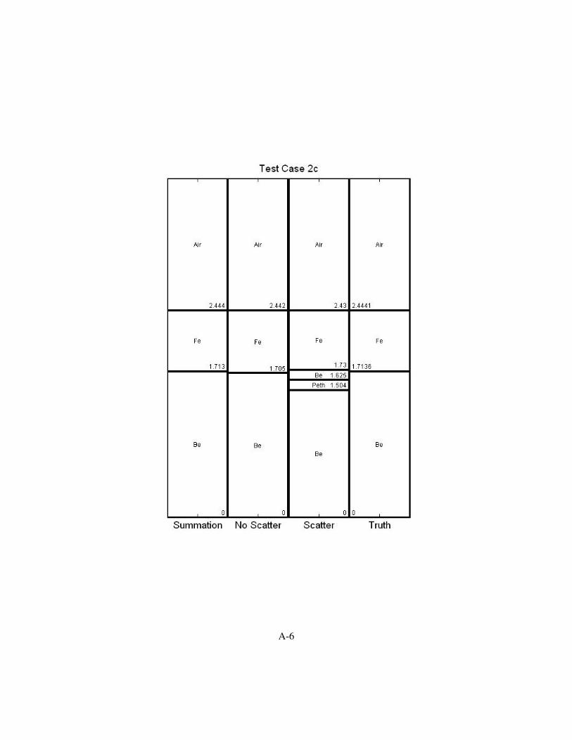
A-6

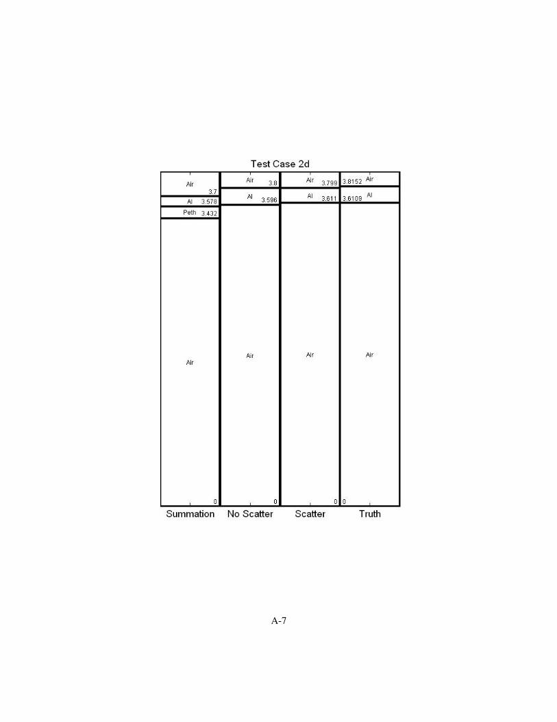
A-7

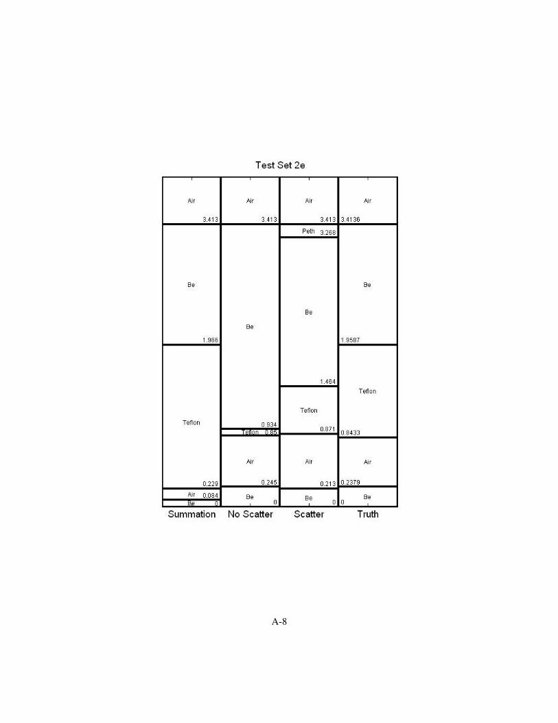
A-8

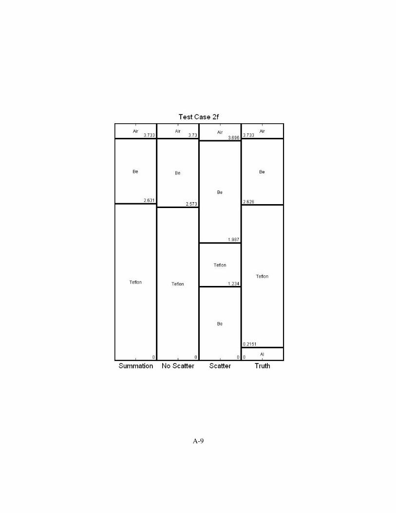
A-9

A-10

A-11

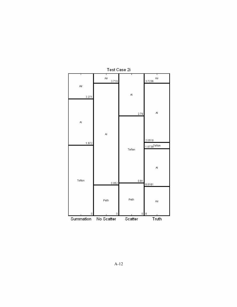
A-12

A-13

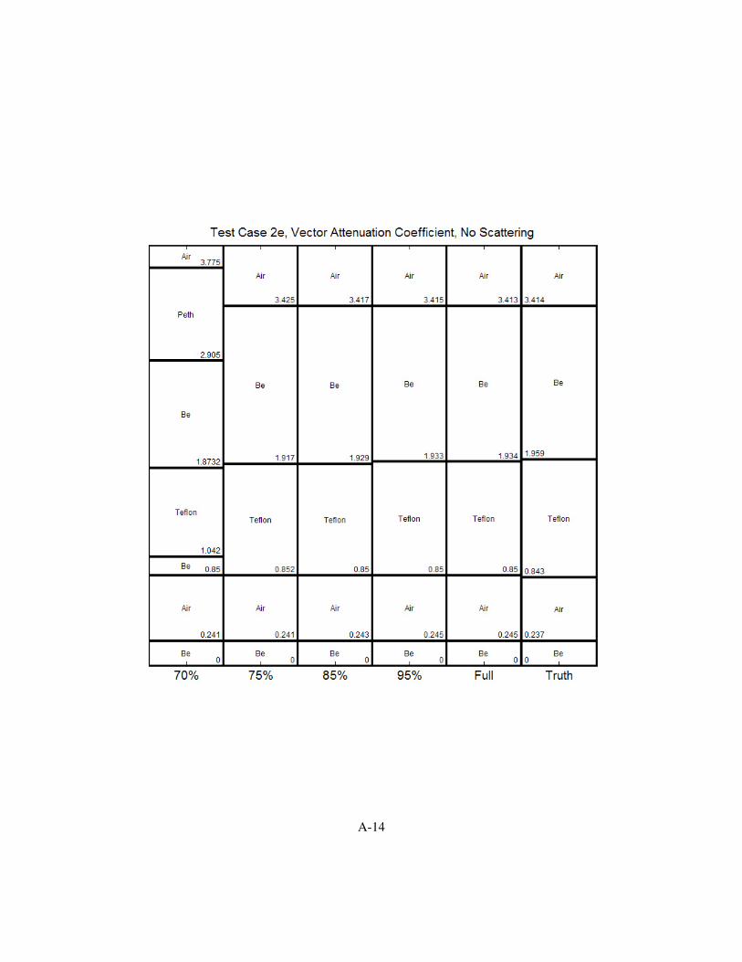
A-14

Appendix B. MATLABr

Code

The following contains the MATLABr

code used to implement the GPS algorithm on LANL

reconstruction problem. The first five files are required by the NOMADm software, while the

last two implement the objective function using the single attenuation coefficient and the vector of

attenuation coefficients, respectively, for each material.

B.1 Main Function File

%**************************************************************************% x_ray: Computes the objective function value for the X-Ray mixed% variable optimization problem% -------------------------------------------------------------------------% Variables:% cx = unused% fx = objective function value% x = layer edge locations (continuous variables)% p = layer materials (catgorical variables)% material = layer materials (polychromatic numerical% values)% n = number of layers% Param = structure containing all paramaters for the% optimization problem% .C = continuous case flag% .cost = cost function being used% .EndEdgeLocation = location of outer edge of last layer% .EndEdgeMaterial = material of last layer (usually air)% .Materials = array of possible material% .mu = array of attenuation coefficients for% possible materials% .Q = Discrete Abel Matrix, data, and coefficient%**************************************************************************

function [fx,cx] = x_ray(x,p);

Param = getappdata(0,’PARAM’);n=p1;

% Set up Cost Function for Continous Caseif Param.C==1;

% Add back removed layer of outer edge materialmaterial = [x(n+1:end); Param.EndEdgeMaterial];x=[x(1:n); Param.EndEdgeLocation];

% Set up Cost Function for Discrete Caseelse

B-1

material=[];p(1)=[];for k=1:n

value=p(k);index=strmatch(value,Param.Materials,’exact’);material = [material; Param.mu(index)];

end

% Add back removed layer of outer edge materialmaterial=[material; Param.mu(strmatch(Param.EndEdgeMaterial,...

Param.Materials,’exact’))];x=[x; Param.EndEdgeLocation];

end

% Increase number of layers to account for adding back removed outer layern=n+1;fx = feval(Param.cost,n,x,material, Param.Q)cx = [];

return

B.2 Parameter File

%**************************************************************************% x_ray_Param: Storage of global data for the optimization problem.% -------------------------------------------------------------------------% Variables:% Materials = cell array of all possible materials that can% be used% MaterialIndex = vector of indices of Materials that will be used% in the run% Param = structure of optimization problem data% .Materials = cell array list of possible layer material% property values for this run% .MaxNumLayers = maximum number of layers allowed% .MinNumLayers = minimum number of layers allowed% .MinLayerWidth = minimum width of each layer% .P_Min = minimum value for x_ray return% .P_Max = maximum value for x_ray return% .L = radiograph size% .C = continuous case flag% .EndEdgeLocation = location of outer edge of last layer% .Materials = array of possible materials% .MaxNumLayers = maximum number of layers% .MinLayerWidth = minimum layer width constraint% .MinNumLayers = minimum number of layers% .P_max = maximum attenuation value, used in continuous% case only% .P_min = minimum attenuation value, used in continuous

B-2

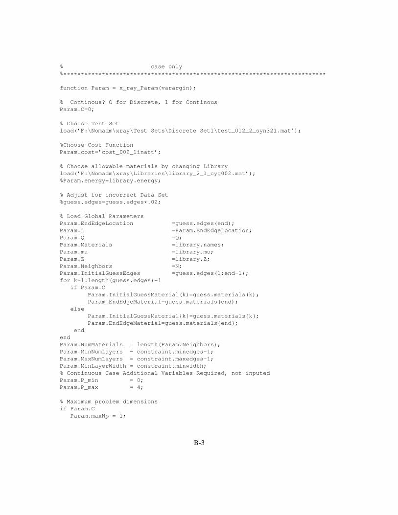
% case only%***************************************************************************

function Param = x_ray_Param(varargin);

% Continous? O for Discrete, 1 for ContinousParam.C=0;

% Choose Test Setload(’F:\Nomadm\xray\Test Sets\Discrete Set1\test_012_2_syn321.mat’);

%Choose Cost FunctionParam.cost=’cost_002_linatt’;

% Choose allowable materials by changing Libraryload(’F:\Nomadm\xray\Libraries\library_2_1_cyg002.mat’);%Param.energy=library.energy;

% Adjust for incorrect Data Set%guess.edges=guess.edges*.02;

% Load Global ParametersParam.EndEdgeLocation =guess.edges(end);Param.L =Param.EndEdgeLocation;Param.Q =Q;Param.Materials =library.names;Param.mu =library.mu;Param.Z =library.Z;Param.Neighbors =N;Param.InitialGuessEdges =guess.edges(1:end-1);for k=1:length(guess.edges)-1

if Param.CParam.InitialGuessMaterial(k)=guess.materials(k);Param.EndEdgeMaterial=guess.materials(end);

elseParam.InitialGuessMaterialk=guess.materialsk;Param.EndEdgeMaterial=guess.materialsend;

endendParam.NumMaterials = length(Param.Neighbors);Param.MinNumLayers = constraint.minedges-1;Param.MaxNumLayers = constraint.maxedges-1;Param.MinLayerWidth = constraint.minwidth;% Continuous Case Additional Variables Required, not inputedParam.P_min = 0;Param.P_max = 4;

% Maximum problem dimensionsif Param.C

Param.maxNp = 1;

B-3

Param.maxNx = 2*Param.MaxNumLayers;else

Param.maxNp = Param.MaxNumLayers;Param.maxNx = Param.MaxNumLayers;

end

% Allow for different initial parameters (Debugging only)!Param.InitialGuessMaterial = ’Fe’;Param.InitialGuessEdges=[2.7];

return

B.3 Initial Iterate File

%**************************************************************************% x_ray_x0: Contains the initial guess information for the X-Ray mixed% variable optimization problem% -------------------------------------------------------------------------% Variables:% iterate = structure of current iterate data% .x = current iterate layer edge locations% (continuous variables)% .p = current iterate layer materials% (catgorical variables)% Param = structure containing all paramaters for% the optimization% .C = continuous case flag% .InitialGuessEdges = layer edge locations initial guess% .InitialGuessMaterial = layer material initial guess%**************************************************************************

function iterate = x_ray_x0

Param = getappdata(0,’PARAM’);

% Original Starting Point Continous Caseif Param.C==1

iterate.x = [Param.InitialGuessEdges’; Param.InitialGuessMaterial’];iterate.p1=length(Param.InitialGuessEdges);

else

% Original starting point Discrete Caseiterate.x = [Param.InitialGuessEdges’];iterate.p1=length(Param.InitialGuessEdges);for k=1:length(Param.InitialGuessEdges);

iterate.pk+1 = Param.InitialGuessMaterialk;end

end

B-4

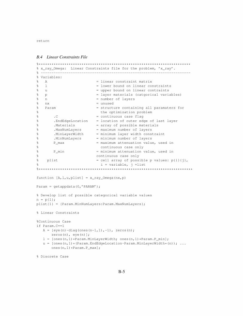
return

B.4 Linear Constraints File

%***********************************************************************% x_ray_Omega: Linear Constraints file for the problem, ’x_ray’.% ----------------------------------------------------------------------% Variables:% A = linear constraint matrix% l = lower bound on linear constraints% u = upper bound on linear contraints% p = layer materials (catgorical variables)% n = number of layers% nx = unused% Param = structure containing all paramaters for% the optimization problem% .C = continuous case flag% .EndEdgeLocation = location of outer edge of last layer% .Materials = array of possible materials% .MaxNumLayers = maximum number of layers% .MinLayerWidth = minimum layer width constraint% .MinNumLayers = minimum number of layers% P_max = maximum attenuation value, used in% continuous case only% P_min = minimum attenuation value, used in% continuous case only% plist = cell array of possible p values: pij,% i = variable, j =list%************************************************************************

function [A,l,u,plist] = x_ray_Omega(nx,p)

Param = getappdata(0,’PARAM’);

% Develop list of possible categorical variable valuesn = p1;plist1 = Param.MinNumLayers:Param.MaxNumLayers;

% Linear Constraints

%Continuous Caseif Param.C==1

A = [eye(n)-diag(ones(n-1,1),-1), zeros(n);zeros(n), eye(n)];

l = [ones(n,1)*Param.MinLayerWidth; ones(n,1)*Param.P_min];u = [ones(n,1)*(Param.EndEdgeLocation-Param.MinLayerWidth*(n)); ...

ones(n,1)*Param.P_max];

% Discrete Case

B-5

elseA = [eye(n)-diag(ones(n-1,1),-1); zeros(1,n-1), 1];l = [ones(n,1)*Param.MinLayerWidth; n*Param.MinLayerWidth];u = [ones(n,1)*(Param.EndEdgeLocation-Param.MinLayerWidth*(n));...

Param.EndEdgeLocation-n*Param.MinLayerWidth];[plist2:n+1] = deal(Param.Materials);

end

return

B.5 Neighborhood Definition File

%**************************************************************************% x_ray_N: User-supplied function defining set of neighbors for a% a given vector of categorical variables p.% -------------------------------------------------------------------------% Variables:% add = addition of layer flag% delete = deletion of layer flag% delta = unused% index = adjacentcy matrix index of material being% considered% innerindex = adjacentcy matrix index of material layer to% the inside of current layer considered% iterate = current iterate for whom discrete neighbor% point will be found.% .p = current iterate layer materials (catgorical% variables)% .x = current iterate layer edge locations(continuo% us variables)% neighbor = iterate who is a neighbor of p% .p = layer materials of iterate who is a neighbor% of p% .x = layer edge location of iterate who is a% neighbor of p% N = vector of iterates who are neighbors of p% NumLayers = number of layers in current iterate% outerindex = adjacentcy matrix index of material layer to% the outside of current layer considered% outerlayerindex = adjacentcy matrix index of outside layer% material (usually 1)% p = temporary iterate layer materials, used for% calculations% Param = structure containing all paramaters for the% optimization% .C = continuous case flag% .Materials = array of possible materials% .MaxNumLayers = maximum number of layers allowed% .MinNumLayers = minimum number of layers

B-6

% .P_max = maximum attenuation value, used in continuous% case only% .P_min = minimum attenuation value, used in continuous% case only% plist = cell array of possible p values: pij,% i = variable, j = list% Problem = unused% x = temporary layer edge locations used for% calculation% y = temporary value used in calculations%%*************************************************************************

function N = x_ray_N(Problem,iterate,plist,delta);

Param = getappdata(0,’PARAM’);NumLayers = iterate.p1;N= [];outerlayerindex=strmatch(Param.EndEdgeMaterial,Param.Materials,’exact’);

% Neighbor Definition for the Continous Caseif Param.C==1

% Include neighbors in which a Layer is addedif (NumLayers < Param.MaxNumLayers)

x=iterate.x;

% Determine value of added layersif x(1) <= Param.P_max/2

x=[0;x(1:NumLayers); Param.P_min; x(NumLayers+1:end)];else

x=[0;x(1:NumLayers); Param.P_max; x(NumLayers+1:end)];end

% Calculate adjacent layer averagesy=[(x(2:NumLayers+1)+x(1:NumLayers))/2; (x(NumLayers+3:end)+...

x(NumLayers+2:end-1))/2];

% Insert Added Layersfor k = NumLayers:-1:1

x=iterate.x;x=[x(1:k-1); y(k); x(k:NumLayers); x(NumLayers+1:...

NumLayers+k-1); y(NumLayers+k); x(NumLayers+k:end)];neighbor.x = x;neighbor.p = iterate.p;neighbor.p1 = NumLayers + 1;N = [N neighbor];

endend

B-7

% Include neighbors in which one edge is removedif (NumLayers > Param.MinNumLayers)

for k = NumLayers:-1:1x=iterate.x;x(NumLayers+k)=[(iterate.x(NumLayers+k)+iterate.x(NumLayers+...

(k+1)))/2];x(NumLayers+k+1)=[];x(k)=[];neighbor.x = x;neighbor.p = iterate.p;neighbor.p1 = NumLayers - 1;N = [N neighbor];

endend

% Neighbor Definitions for the Discrete Caseelse

% Include neighbors in which one material layer is removedif NumLayers > Param.MinNumLayers

for k = NumLayers:-1:1p=iterate.p;delete=0;p(1)=[];index=strmatch(p(k),Param.Materials,’exact’);

% Case if outermost layerif k==NumLayers

innerindex=strmatch(p(k-1),Param.Materials,’exact’);if (Param.Neighbors(index, innerindex)==1 && innerindex=...

=outerlayerindex)if NumLayers > 2

delete=2;end

elseif (Param.Neighbors(index, innerindex)==1 | ...Param.Neighbors(index, outerlayerindex)==1)

delete=1;end

% Case if inner most layerelseif k==1

outerindex=strmatch(p(k+1),Param.Materials,’exact’);if Param.Neighbors(index, outerindex)==1

delete=1;end

% Other caseselse

innerindex=strmatch(p(k-1),Param.Materials,’exact’);outerindex=strmatch(p(k+1),Param.Materials,’exact’);

B-8

if Param.Neighbors(index, outerindex)==1 | Param.Neighbors...(index, innerindex)==1

delete=1;end

end

% Delete a layerif delete==1

x=iterate.x;x(k)=[];neighbor.x=x;neighbor.p = iterate.p;neighbor.p1 = NumLayers - 1;neighbor.p(k+1) = [];N = [N neighbor];

elseif delete==2x=iterate.x;x(k-1:k)=[];neighbor.x=x;neighbor.p=iterate.p;neighbor.p1=NumLayers - 2;neighbor.p(k:k+1)=[];N= [N neighbor];

endend

end

% Include neighbors in which 1 material layer is swapedfor k = NumLayers:-1:1

x=iterate.x;p=iterate.p;p(1)=[];index=strmatch(p(k),Param.Materials,’exact’);% Check all materialsfor i=1:Param.NumMaterials

%Prevent outermost layer from being duplicatedif (˜(k==NumLayers) | ˜(i==outerlayerindex))

if Param.Neighbors(index, i)==1neighbor.x = iterate.x;neighbor.p = iterate.p;neighbor.pk+1 = Param.Materialsi;N = [N neighbor];

endend

endend

% Include neighbors in which 1 material layer is addedif NumLayers < Param.MaxNumLayers

B-9

% Calculate adjacent layer averagesx=iterate.x;p=iterate.p;x=[0;x(1:NumLayers);Param.EndEdgeLocation];y=[(x(2:NumLayers+2)+x(1:NumLayers+1))/2];

% Check for all layersfor k = NumLayers+1:-1:1

x=iterate.x;p=iterate.p;x=[x(1:k-1);y(k);x(k:NumLayers)];% Check all materialsfor i=1:Param.NumMaterials

add=0;

% Outermost Layer caseif k==NumLayers+1

innerindex=strmatch(p(k),Param.Materials,’exact’);if (Param.Neighbors(i, innerindex)==1 | ...

Param.Neighbors(i, outerlayerindex)==1)add=1;

end

% Innermost Layer caseelseif k==1

outerindex=strmatch(p(k+1),Param.Materials,’exact’);if Param.Neighbors(i, outerindex)==1

add=1;end

% Other caseselse

innerindex=strmatch(p(k),Param.Materials,’exact’);outerindex=strmatch(p(k+1),Param.Materials,’exact’);if Param.Neighbors(i, outerindex)==1 | ...

Param.Neighbors(i, innerindex)==1add=1;

endend

% Add a layerif add==1;

neighbor.x = x;neighbor.p = iterate.p;neighbor.p=NumLayers+1, iterate.p2:k, ...

Param.Materialsi, iterate.pk+1:end;N = [N neighbor];

endend

end

B-10

endend

return

B.6 Objective Function 1 File

%*************************************************************************% cost_002_linatt is a cost functional evaluation for% use with the mixed-variable optimization X-ray inversion% project. It assumes an attenuation reconstruction% from normalized transmission data. The norm assumes% Guassian additive noise.%% This function differs from cost_001_linatt only in the% last line -- here we use a data fidelity norm on the% logarithm of the data%% USAGE:% [cost] = cost_002_linatt(n,e,p,Q)%% INPUTS:% [The inputs constitute an object description]% Q1 = P is the Abel projection operator scaled to% unit data pixel size% Q2 = data is the vector of transmission data values% ordered from inside outward. Values are assumed% to be normalized to unity for zero attenuation.% Q3 = w is the pixel width (and height) on the% detector in real units.% n is the integer number of edges in the object% The edge of the data is included as an edge location.% e is a vector of ring edge locations ordered from% inside outward. The units are pixels. The last% value must be equal to the number of data pixels.% p is a vector of ring material property values (one% for each ring). In this case, p is a vector of% attenuation values.%% OUTPUTS:% cost is the function evaluation or cost.%*************************************************************************

function [cost] = cost_002_linatt(n,e,p,Q)

% set up some stuffP=Q1;data=Q2(:);w=Q3;

B-11

nd=length(data);

% Contstruct a pixelized version of the object (u)% (convert (n,t,p) into a vector of length nd)

edges=[0;e(:)]/w;temp=repmat(1:nd,n+1,1)-repmat(edges,1,nd);x=-diff(min(max(temp,0),1));uparts=x.*repmat(p(:),1,nd);u=(sum(uparts))’;

% Compute the costcost = norm(-P*u/wˆ2-log(data),2)/sqrt(nd);

return

B.7 Objective Function 2 File

%*************************************************************************% cost_004_linatt is a cost functional evaluation for% use with the mixed-variable optimization X-ray inversion% project. It assumes an attenuation reconstruction% from normalized energy transmission data. The norm assumes% Guassian additive noise.%% This function differs from cost_001_linatt only in the% last line -- here we use a data fidelity norm on the% logarithm of the data%% USAGE:% [cost] = cost_004_linatt(n,e,p,Q)%% INPUTS:% [The inputs constitute an object description]% Q1 = P is the Abel projection operator scaled to% unit data pixel size% Q2 = data is the vector of transmission data values% ordered from inside outward. Values are assumed% to be normalized to unity for zero attenuation.% Q3 = w is the pixel width (and height) on the% detector in real units.% Q4 = energy is a vector of intensity normalized% energy values describing the source spectrum% n is the integer number of edges in the object% The edge of the data is included as an edge location.% e is a vector of ring edge locations ordered from% inside outward. The units are pixels. The last% value must be equal to the number of data pixels.% mu is a matrix of material property values (one row

B-12

% for each ring). In this case, p is a matrix of% attenuation values such that p(i,j) is the attenuation% factor for ring j at the ith energy.% energy is a vector of energy values corresponding to% the attenuation value columns in mu. The energy is% spectrum intensity normalized so that sum(energy)=1.%% OUTPUTS:% cost is the function evaluation or cost.%*************************************************************************

function [cost] = cost_004_linatt(n,e,mu,energy,Q)

% set up some stuffP=Q1;data=Q2(:);w=Q3;nd=length(data);

%%%%% Construct the material ID object %%%%%e=e/w;temp=repmat(1:nd,n+1,1)-repmat([0;e(:)],1,nd);objMID=-diff(min(max(temp,0),1));

%%% Construct attenuation objects for each energyfor j=1:length(energy)

objMU(j,:)=sum(repmat(mu(:,j),1,nd).*objMID);end

%%% Calculate the projectionE=zeros(nd,1);for j=1:length(energy)

E=E+energy(j)*exp(-(P*objMU(j,:)’/wˆ2));end

% Compute the costcost = norm(log(E)-log(data),2)/sqrt(nd);

return

B-13

Bibliography

[1] Aarts, E. and J. K. Lenstra (editors). Local Search in Combinatorial Optimization. PrincetonUniversity Press, New York, 1991.

[2] Abel, N. H. “Auflosung einer mechanischen Aufgabe”. Math, 1:153–157, 1826.

[3] Abramson, M. A. “NOMADm optimization software”. http://www.afit.edu/en/ENC/Faculty/-MAbramson/NOMADm.html.

[4] Abramson, M. A. Pattern Search Algorithms for Mixed Variable General Constrained Op-timization Problems. Ph.D. thesis, Department of Computational and Applied Mathematics,Rice University, August 2002.

[5] Abramson, M. A. “Mixed variable optimization of a load-bearing thermal insulation systemusing a filter pattern search algorithm”. Optimization and Engineering, 5(2):157–177, 2004.

[6] Abramson, M. A. “Second-Order Behavior of Pattern Search”. SIAM Journal on Optimiza-tion, 16(2):315–330, 2005.

[7] Abramson, M. A. and C. Audet. Second-order convergence of mesh adaptive direct search.Technical Report TR05-09, Department of Computational and Applied Mathematics, RiceUniversity, Houston Texas, 2005.

[8] Abramson, M. A., C. Audet, and J. E. Dennis, Jr. “Generalized Pattern Searches with Deriva-tive Information”. Mathematical Programming, Series B, 100(1):3–25, 2004.

[9] Abramson, M. A., C. Audet, and J. E. Dennis, Jr. On the convergence of filter pattern searchalgorithms for mixed variable constrained optimization problems. Technical Report TR04-09, Department of Computational and Applied Mathematics, Rice University, Houston Texas,2004.

[10] Abramson, M. A., O. A. Brezhneva, and J.E. Dennis Jr. Pattern Search in the Presence ofDegeneracy. Technical Report TR03-09, Department of Computational and Applied Mathe-matics, Rice University, Houston Texas, 2005.

[11] Alberto, P., F. Nogueira, U. Rocha, and L. N. Vicente. “Pattern Search Methods for user-provided points: application to molecular geometry problems”. SIAM Journal on Optimiza-tion., 14(4):1216–1236, 2004.

[12] Asaki, T. J. Inverse Abel Transform Regularization. Technical Report LA–UR–04–4100, LosAlamos National Laboratory, Los Alamos National Laboratory, Los Alamos, New Mexico87545, 2004.

[13] Asaki, T. J. Optimization-Based Forward Measurement Operator Tomography. Technical Re-port LA–UR–05–2658, Los Alamos National Laboratory, Los Alamos National Laboratory,Los Alamos, New Mexico 87545, 2005.

BIB-1

[14] Asaki, T. J., P. R. Campbell, R. Chartrand, C. Powell, K. R. Vixie, and B. Wohlberg. AbelInversion Using Total Variation Regularization: Applications. Technical Report LA-UR-05-2657, Los Alamos National Laboratory, Los Alamos National Laboratory, Los Alamos, NewMexico 87545, April 2005.

[15] Asaki, T. J., R. Chartrand, K. R. Vixie, and B. Wohlerg. “Abel Iversion using Total-VariationRegularization”. Inverse Problems, 21:1895–1903, 2005.

[16] Audet, C. and J. E. Dennis, Jr. “Pattern Search Algorithms for Mixed Variable Programming”.SIAM Journal on Optimization, 11(3):573–594, 2000.

[17] Audet, C. and J. E. Dennis, Jr. “Analysis of Generalized Pattern Searches”. SIAM Journal onOptimization, 13(3):889–903, 2003.

[18] Audet, C. and J. E. Dennis, Jr. “Mesh Adaptive Direct Search Algorithms for ConstrainedOptimization”. SIAM Journal on Optimization, To appear, 2004.

[19] Audet, C. and J. E. Dennis, Jr. “A Pattern Search Filter Method for Nonlinear ProgrammingWithout Derivatives”. SIAM Journal on Optimization, 14(4):980–1010, 2004.

[20] Booker, A. J., J. E. Dennis, Jr., P. D. Frank, D. B. Serafini, V. Torczon, and M. W. Trosset.“A Rigorous Framework for Optimization of Expensive Functions by Surrogates”. StructuralOptimization, 17(1):1–13, February 1999.

[21] Box, G. E. P. “Evolutionary Operation: A Method for Increasing Industrial Productivity”.Applied Statistics, 6(2):81–101, 1957.

[22] Clarke, F. H. Optimization and Nonsmooth Analysis. Wiley, New York, 1983. Reissued in1990 by SIAM Publications, Philadelphia, as Vol. 5 in the series Classics in Applied Mathe-matics.

[23] Conn, A. R., N. I. M. Gould, and P. L. Toint. “A Globally Convergent Augmented LagrangianAlgorithm for Optimization With General Constraints and Simple Bounds”. SIAM Journalon Numerical Analysis, 28(2):545–572, April 1991.

[24] Cremers, C. J. and R. C. Birkebak. “Application of the Abel Integral Equation to Spectro-graphic Data”. Applied Optics, 5(6):1057–1063, 1966.

[25] Davis, C. “Theory of Positive Linear Dependence”. American Journal of Mathematics,76(4):733–746, 1954.

[26] De Jong, Kenneth A. An Analysis of the Behavior of a Class of Genetic Adaptive Systems.Ph.D. thesis, University of Michigan, Ann Arbor, 1975.

[27] Dennis, Jr., J. E. and V. Torczon. “Direct Search Methods on Parallel Machines”. SIAMJournal on Optimization, 1(4):448–474, 1991.

[28] Dolan, E. D., R. M. Lewis, and V. Torczon. “On the Local Convergence Properties of PatternSearch”. SIAM Journal on Optimization, 14(4):567–583, 2004.

BIB-2

[29] Fletcher, R. and S. Leyffer. “Nonlinear Programming Without a Penalty Function”. Mathe-matical Programming, Series A, 91(2):239–269, 2002.

[30] Glover, F. “Tabu Search–Part I”. ORSA Journal on Computing, 1(3):190–206, 1989.

[31] Glover, F. “Tabu Search–Part II”. ORSA Journal on Computing, 2(1):4–32, 1990.

[32] Hilal, M. A. and R. W. Boom. “Optimization of Mechanical Supports for Large Supercon-ductive Magnets”. Advances in Cryogenic Engineering, 22:224–232, 1977.

[33] Hooke, R. and T. A. Jeeves. “Direct Search Solution of Numerical and Statistical Problems”.Journal of the Association for Computing Machinery, 8(2):212–229, 1961.

[34] Kak, A. C. and M. Slaney. Principles of Computerized Tomographic Imaging. IEEE Press,Inc., New York, 1991.

[35] Karush, W. Minima of Functions of Several Variables with Inequalities as side conditions.Master’s thesis, Department of Mathematics, University of Chicago, 1939.

[36] Kirkpatrick, S., C. D. Gelatt, and M. P. Vecchi. “Optimization by Simulated Annealing”.Science, 220(4598):671–680, 1983.

[37] Kokkolaras, M., C. Audet, and J. E. Dennis, Jr. “Mixed variable optimization of the num-ber and composition of heat intercepts in a thermal insulation system”. Optimization andEngineering, 2(1):5–29, 2001.

[38] Kolda, T. G., R. M. Lewis, and V. Torczon. “Optimization by direct search: new perspectiveson some classical and modern methods”. SIAM Review, 45(3):385–482, 2003.

[39] Kuhn, H. W. and A.W. Tucker. “Nonlinear Programmming”. University of California Press,Berkely, CA, 1951.

[40] Lewis, R. M. and V. Torczon. Rank Ordering and Positive Bases in Pattern Search Algorithms.Technical Report 96–71, Institute for Computer Applications in Science and Engineering,Mail Stop 132C, NASA Langley Research Center, Hampton, Virginia 23681–2199, 1996.

[41] Lewis, R. M. and V. Torczon. “Pattern Search Algorithms for Bound Constrained Minimiza-tion”. SIAM Journal on Optimization, 9(4):1082–1099, 1999.

[42] Lewis, R. M. and V. Torczon. “Pattern Search Methods for Linearly Constrained Minimiza-tion”. SIAM Journal on Optimization, 10(3):917–941, 2000.

[43] Lewis, R. M. and V. Torczon. “A Globally Convergent Augmented Lagrangian Pattern SearchAlgorithm for Optimization With General Constraints and Simple Bounds”. SIAM Journalon Optimization, 12(4):1075–1089, 2002.

[44] Lucidi, S. and V. Piccialli. “A Derivative-Based Algorithm for a Particular Class of MixedVariable Optimization Problems”. Optimization Methods and Software, 17(3–4):317–387,2004.

BIB-3

[45] Lucidi, S., V. Piccialli, and M. Sciandrone. “An Algorithm Model for Mixed Variable Pro-gramming”. SIAM Journal on Optimization, 15(4):1057–1084, 2005.

[46] Maldonado, C. D., A. P. Caron, and H. N. Olsen. “New Method for Obtaining EmissionCoefficients from Emitted Intensities: Circularly Symmetric Light Sources”. Journal of OpticSociety of America, 55:1247–1254, 1965.

[47] Nash, S. G. and A. Sofer. Linear and Nonlinear Programming. McGraw–Hill, New York,1996.

[48] Polak, E. and M. Wetter. “Precision Control for Generalized Pattern Search Algorithms withAdaptive Precision Function Evaluations”. SIAM Journal on Optimization, 16(3):650–669,2006.

[49] Smith, L. M., D. R. Keefer, and S. I. Sudharsanan. “Abel Inversion using Transform Tech-niques”. Journal of Quantitative Spectroscopy and Radiation Transfer, 39:367–373, 1988.

[50] Sriver, T. A., J. W. Chrissis, and M.A. Abramson. “Pattern Search Ranking and SelectionAlgorithms for Mixed Variable Stochastic Optimization”. 2004. Preprint.

[51] Torczon, V. “On the Convergence of Pattern Search Algorithms”. SIAM Journal on Opti-mization, 7(1):1–25, February 1997.

BIB-4

Vita

Second Lieutenant Kevin R. O’Reilly graduated from East Brunswick High School in East

Brunswick, New Jersey. He entered undergraduate studies at the United States Air Force Academy

in Colorado Springs, Colorado where he graduated with a Bachelor of Science degree in Space

Operations in June 2004 and was recognized as a Distinguished Graduate. Following graduation he

was commissioned an officer in the United States Air Force and was assigned to Wright-Patterson

AFB where he entered the Graduate School of Engineering and Management, Air Force Institute

of Technology to pursue a Masters of Science degree in Space Systems. Upon graduation, he will

be assigned to Vandenberg AFB, California where he will receive technical training in the Space

and Missile career field in order to become a space and missile operator.

VITA-1

REPORT DOCUMENTATION PAGE Form Approved OMB No. 074-0188

The public reporting burden for this collection of information is estimated to average 1 hour per response, including the time for reviewing instructions, searching existing data sources, gathering and maintaining the data needed, and completing and reviewing the collection of information. Send comments regarding this burden estimate or any other aspect of the collection of information, including suggestions for reducing this burden to Department of Defense, Washington Headquarters Services, Directorate for Information Operations and Reports (0704-0188), 1215 Jefferson Davis Highway, Suite 1204, Arlington, VA 22202-4302. Respondents should be aware that notwithstanding any other provision of law, no person shall be subject to an penalty for failing to comply with a collection of information if it does not display a currently valid OMB control number. PLEASE DO NOT RETURN YOUR FORM TO THE ABOVE ADDRESS. 1. REPORT DATE (DD-MM-YYYY) 23-03-2006

2. REPORT TYPE Master’s Thesis

3. DATES COVERED (From – To) 24-08-2004 – 23-03-2006

5a. CONTRACT NUMBER

5b. GRANT NUMBER

4. TITLE AND SUBTITLE Quantitative Object Reconstruction using Abel Transform Tomography and Mixed Variable Optimization

5c. PROGRAM ELEMENT NUMBER

5d. PROJECT NUMBER 2005-159 5e. TASK NUMBER

6. AUTHOR(S) O’Reilly, Kevin, R., Second Lieutenant, USAF

5f. WORK UNIT NUMBER

7. PERFORMING ORGANIZATION NAMES(S) AND ADDRESS(S) Air Force Institute of Technology Graduate School of Engineering and Management (AFIT/EN) 2950 Hobson Way WPAFB OH 45433-7765

8. PERFORMING ORGANIZATION REPORT NUMBER AFIT/GSS/ENC/06-1

10. SPONSOR/MONITOR’S ACRONYM(S) LANL

9. SPONSORING/MONITORING AGENCY NAME(S) AND ADDRESS(ES) Los Alamos National Laboratory Attn: Dr. Thomas J. Asaki CCS-2, Mail Stop D413 Los Alamos NM 87545 Comm: (505)-667-5787

11. SPONSOR/MONITOR’S REPORT NUMBER(S)

12. DISTRIBUTION/AVAILABILITY STATEMENT APPROVED FOR PUBLIC RELEASE; DISTRIBUTION UNLIMITED.

13. SUPPLEMENTARY NOTES 14. ABSTRACT Researchers at the Los Alamos National Laboratory (LANL) are interested in quantitatively reconstructing an object using Abel transform x-ray tomography. Specifically, they obtain a radiograph by x-raying an object and attempt to quantitatively determine the number and types of materials and the thickness of each material layer. Their current methodologies either fail to provide a quantitative description of the object or are generally too slow to be useful in practice. As an alternative, the problem is model here as a mixed variable programming (MVP) problem, in which some variables are nonnumeric and for which no derivative information is available. The generalized pattern search (GPS) algorithm for linearly constrained MVP problems is applied to the x-ray tomography problem, by means of the NOMADm MATLAB® software package. Numerical results are provided for several test configurations of cylindrically symmetrical objects and show that, while there are difficulties to be overcome by researchers at LANL, this method is promising for solving x-ray tomography object reconstruction problems in practice. 15. SUBJECT TERMS X-ray Tomography, Abel Transform, Mixed Variable Programming, Pattern Search Algorithms, Constrained Optimization, Quantitative Object Reconstruction 16. SECURITY CLASSIFICATION OF:

19a. NAME OF RESPONSIBLE PERSON LtCol Mark A. Abramson

REPORT

U ABSTRACT

U c. THIS PAGE

U

17. LIMITATION OF ABSTRACT UU

18. NUMBER OF PAGES 97 19b. TELEPHONE NUMBER (Include area code)

(937) 255-3636, ext 4524;mark.abramson@afit.edu Standard Form 298 (Rev: 8-98) Prescribed by ANSI Std. Z39-18