air force institute of technology · alkali laser; a three level numerical approach ......
TRANSCRIPT

SIMULATION OF A DIODE PUMPEDALKALI LASER; A THREE LEVEL
NUMERICAL APPROACH
THESIS
Shawn W. Hackett, Second Lieutenant, USAF
AFIT/GAP/ENP/10-M06
DEPARTMENT OF THE AIR FORCEAIR UNIVERSITY
AIR FORCE INSTITUTE OF TECHNOLOGY
Wright-Patterson Air Force Base, Ohio
APPROVED FOR PUBLIC RELEASE; DISTRIBUTION UNLIMITED.

The views expressed in this thesis are those of the author and do not reflect theofficial policy or position of the United States Air Force, Department of Defense, orthe United States Government.

AFIT/GAP/ENP/10-M06
SIMULATION OF A DIODE PUMPED ALKALI LASER; A THREE LEVEL
NUMERICAL APPROACH
THESIS
Presented to the Faculty
Department of Engineering Physics
Graduate School of Engineering and Management
Air Force Institute of Technology
Air University
Air Education and Training Command
in Partial Fulfillment of the Requirements for the
Degree of Master of Science in Applied Physics
Shawn W. Hackett, BS
Second Lieutenant, USAF
March 2010
APPROVED FOR PUBLIC RELEASE; DISTRIBUTION UNLIMITED.

AFIT/GAP/ENP/10-M06
SIMULATION OF A DIODE PUMPED ALKALI LASER; A THREE LEVEL
NUMERICAL APPROACH
Shawn W. Hackett, BSSecond Lieutenant, USAF
Approved:
Jeremy C. Holtgrave (Chairman) Date
Glen P. Perram (Member) Date
Kevin C. Gross (Member) Date

AFIT/GAP/ENP/10-M06
Abstract
This paper develops a three level model for a continuous wave diode pumped alkali
laser by creating rate equations based on a three level system. The three level system
consists of an alkali metal vapor, typically Rb or Cs, pumped by a diode from the 2S 12
state to the 2P 32, a collisional relaxation from 2P 3
2to 2P 1
2, and then lasing from 2P 1
2
to 2S 12. The hyperfine absorption and emission cross sections for these transitions are
developed in detail. Differential equations for intra-gain pump attenuation and intra-
gain laser growth are developed in the fashion done by Rigrod. Using Mathematica
7.0, these differential equations are solved numerically and a diode pumped alkali laser
system is simulated. The solutions of the differential equations are then utilized to
characterize the inversion, the gain profile, the output laser intensity, and the pump
intensity absorption profile for many different diode pumped alkali laser systems.
The results of the simulation are compared to previous experimental results and
to previous computational results for similar systems. The absorption profile for
the three level numerical model is shown to have excellent agreement with previous
absorption models. The lineshapes of the three level numerical model are found to
be nearly identical to previous developments excepting those models assumptions.
The three level numerical model provides results closer to experimental results than
previous systems and provides results which observe effects not previously modeled,
such as the effects of lasing on pump attenuation.
iv

Table of Contents
Page
Abstract . . . . . . . . . . . . . . . . . . . . . . . . . . . . . . . . . . . . . . . . . . . . . . . . . . . . . . . . . . . . . . . iv
Table of Contents . . . . . . . . . . . . . . . . . . . . . . . . . . . . . . . . . . . . . . . . . . . . . . . . . . . . . . . . v
List of Figures . . . . . . . . . . . . . . . . . . . . . . . . . . . . . . . . . . . . . . . . . . . . . . . . . . . . . . . . . vii
List of Tables . . . . . . . . . . . . . . . . . . . . . . . . . . . . . . . . . . . . . . . . . . . . . . . . . . . . . . . . . . . ix
List of Symbols . . . . . . . . . . . . . . . . . . . . . . . . . . . . . . . . . . . . . . . . . . . . . . . . . . . . . . . . . . x
I. INTRODUCTION . . . . . . . . . . . . . . . . . . . . . . . . . . . . . . . . . . . . . . . . . . . . . . . . . . . 1
II. BACKGROUND . . . . . . . . . . . . . . . . . . . . . . . . . . . . . . . . . . . . . . . . . . . . . . . . . . . . 4
2.1 Overview . . . . . . . . . . . . . . . . . . . . . . . . . . . . . . . . . . . . . . . . . . . . . . . . . . . . . . . 42.2 Experimental DPAL Development . . . . . . . . . . . . . . . . . . . . . . . . . . . . . . . . . 62.3 Hager Model . . . . . . . . . . . . . . . . . . . . . . . . . . . . . . . . . . . . . . . . . . . . . . . . . . . . 72.4 Lewis Model . . . . . . . . . . . . . . . . . . . . . . . . . . . . . . . . . . . . . . . . . . . . . . . . . . . . 8
III. DPAL Theory and Model . . . . . . . . . . . . . . . . . . . . . . . . . . . . . . . . . . . . . . . . . . . . 10
3.1 Overview . . . . . . . . . . . . . . . . . . . . . . . . . . . . . . . . . . . . . . . . . . . . . . . . . . . . . . 103.2 Three Level System . . . . . . . . . . . . . . . . . . . . . . . . . . . . . . . . . . . . . . . . . . . . . 103.3 Cross sections and Lineshapes for DPALs . . . . . . . . . . . . . . . . . . . . . . . . . . 143.4 Alkali and Collision Partner Properties . . . . . . . . . . . . . . . . . . . . . . . . . . . . 233.5 Lasing and Pump Intensities . . . . . . . . . . . . . . . . . . . . . . . . . . . . . . . . . . . . . 25
IV. Simulation Description . . . . . . . . . . . . . . . . . . . . . . . . . . . . . . . . . . . . . . . . . . . . . . 28
4.1 Overview . . . . . . . . . . . . . . . . . . . . . . . . . . . . . . . . . . . . . . . . . . . . . . . . . . . . . . 284.2 Assumptions . . . . . . . . . . . . . . . . . . . . . . . . . . . . . . . . . . . . . . . . . . . . . . . . . . . 284.3 Simulation Input Parameters . . . . . . . . . . . . . . . . . . . . . . . . . . . . . . . . . . . . . 294.4 Simulation Outline . . . . . . . . . . . . . . . . . . . . . . . . . . . . . . . . . . . . . . . . . . . . . 304.5 Simulation Outputs . . . . . . . . . . . . . . . . . . . . . . . . . . . . . . . . . . . . . . . . . . . . . 31
V. Results and Simulation Comparisons . . . . . . . . . . . . . . . . . . . . . . . . . . . . . . . . . . 34
5.1 Chapter Overview . . . . . . . . . . . . . . . . . . . . . . . . . . . . . . . . . . . . . . . . . . . . . . 345.2 Comparison to Lewis Model . . . . . . . . . . . . . . . . . . . . . . . . . . . . . . . . . . . . . 34
5.2.1 Inputs . . . . . . . . . . . . . . . . . . . . . . . . . . . . . . . . . . . . . . . . . . . . . . . . . . 345.2.2 Cross Section Broadening Comparison . . . . . . . . . . . . . . . . . . . . . . . 355.2.3 Absorption Profile Comparison . . . . . . . . . . . . . . . . . . . . . . . . . . . . . 36
v

Page
5.3 Comparison to Hager Model . . . . . . . . . . . . . . . . . . . . . . . . . . . . . . . . . . . . . 415.3.1 Spectral Profile Comparison . . . . . . . . . . . . . . . . . . . . . . . . . . . . . . . 41
5.4 CW Simulation of a Pulsed System . . . . . . . . . . . . . . . . . . . . . . . . . . . . . . . 465.5 Simulation of a System Near Threshold . . . . . . . . . . . . . . . . . . . . . . . . . . . . 50
VI. Conclusions . . . . . . . . . . . . . . . . . . . . . . . . . . . . . . . . . . . . . . . . . . . . . . . . . . . . . . . 53
6.1 Comparison to Other Models . . . . . . . . . . . . . . . . . . . . . . . . . . . . . . . . . . . . 536.2 Use as a Research Tool . . . . . . . . . . . . . . . . . . . . . . . . . . . . . . . . . . . . . . . . . . 536.3 Future Model Development . . . . . . . . . . . . . . . . . . . . . . . . . . . . . . . . . . . . . . 54
6.3.1 Mode Volume . . . . . . . . . . . . . . . . . . . . . . . . . . . . . . . . . . . . . . . . . . . . 546.3.2 Pulsed DPAL Systems . . . . . . . . . . . . . . . . . . . . . . . . . . . . . . . . . . . . 54
A. Mathematica Code to Solve Rate Equations . . . . . . . . . . . . . . . . . . . . . . . . . . . 55
B. Three Level DPAL Model Notebook for RbSample Input and Without Sample Output . . . . . . . . . . . . . . . . . . . . . . . . . . . . 64
Bibliography . . . . . . . . . . . . . . . . . . . . . . . . . . . . . . . . . . . . . . . . . . . . . . . . . . . . . . . . . . . 97
vi

List of Figures
Figure Page
1. The three level chemical kinetics used for thedevelopment of the DPAL model . . . . . . . . . . . . . . . . . . . . . . . . . . . . . . . . . . 12
2. The D1 manifold for 133Cs without possible transitionslisted . . . . . . . . . . . . . . . . . . . . . . . . . . . . . . . . . . . . . . . . . . . . . . . . . . . . . . . . . 17
3. The D2 manifold for 133Cs without possible transitionslisted . . . . . . . . . . . . . . . . . . . . . . . . . . . . . . . . . . . . . . . . . . . . . . . . . . . . . . . . . 18
4. The D1 manifold for 85Rb without possible transitionslisted . . . . . . . . . . . . . . . . . . . . . . . . . . . . . . . . . . . . . . . . . . . . . . . . . . . . . . . . . 19
5. The D2 manifold for 85Rb without possible transitionslisted . . . . . . . . . . . . . . . . . . . . . . . . . . . . . . . . . . . . . . . . . . . . . . . . . . . . . . . . . 20
6. The D1 manifold for 87Rb without possible transitionslisted . . . . . . . . . . . . . . . . . . . . . . . . . . . . . . . . . . . . . . . . . . . . . . . . . . . . . . . . . 21
7. The D2 manifold for 87Rb without possible transitionslisted . . . . . . . . . . . . . . . . . . . . . . . . . . . . . . . . . . . . . . . . . . . . . . . . . . . . . . . . . 22
8. The architecture used to develop the simulation of theDPAL model . . . . . . . . . . . . . . . . . . . . . . . . . . . . . . . . . . . . . . . . . . . . . . . . . . . 32
9. σ31 for 100 Torr helium and 100 Torr methane fromthe Lewis model [5] . . . . . . . . . . . . . . . . . . . . . . . . . . . . . . . . . . . . . . . . . . . . . 36
10. σ31 for 1000 Torr helium and 1000 Torr methane fromthe Lewis model [5] . . . . . . . . . . . . . . . . . . . . . . . . . . . . . . . . . . . . . . . . . . . . . 37
11. σ31 for 100 Torr helium and 100 Torr methane fromthe three level numerical model . . . . . . . . . . . . . . . . . . . . . . . . . . . . . . . . . . . 37
12. σ31 for 1000 Torr helium and 1000 Torr methane fromthe three level numerical model . . . . . . . . . . . . . . . . . . . . . . . . . . . . . . . . . . . 38
13. The Lewis model 3D absorption profile without lasingfor inputs of Table 6 . . . . . . . . . . . . . . . . . . . . . . . . . . . . . . . . . . . . . . . . . . . . 39
14. The three level numerical model 3D absorption profilewithout lasing for inputs of Table 6 . . . . . . . . . . . . . . . . . . . . . . . . . . . . . . . 40
vii

Figure Page
15. The Lewis model 3D absorption profile with QTLAlasing inputs of Table 6 . . . . . . . . . . . . . . . . . . . . . . . . . . . . . . . . . . . . . . . . . . 42
16. The three level numerical model 3D absorption profilewith lasing for inputs of Table 6 . . . . . . . . . . . . . . . . . . . . . . . . . . . . . . . . . . 43
17. The three level numerical model determination of γ(z)for inputs of Table 6 within the lasing region . . . . . . . . . . . . . . . . . . . . . . . 44
18. The hyperfine absorption profile for the Rb. D1manifold offset by ν21 [3] . . . . . . . . . . . . . . . . . . . . . . . . . . . . . . . . . . . . . . . . . 45
19. The three level numerical model lineshape for the Rb.D1 manifold offset by ν21 . . . . . . . . . . . . . . . . . . . . . . . . . . . . . . . . . . . . . . . . 45
20. The lineshape g31 with the pump lineshape gp overlayedto show the degree of area matching . . . . . . . . . . . . . . . . . . . . . . . . . . . . . . . 48
21. The intensity of the pump (IP ) as it propagates throughthe cell . . . . . . . . . . . . . . . . . . . . . . . . . . . . . . . . . . . . . . . . . . . . . . . . . . . . . . . 48
22. The gain γ as a function of z. . . . . . . . . . . . . . . . . . . . . . . . . . . . . . . . . . . . . 49
23. The Integrated Plus Wave Intensity(upper) and MinusWave Intensity(lower) as functions of z . . . . . . . . . . . . . . . . . . . . . . . . . . . . 49
24. The laser output intensity’s spectral width within thepump profile . . . . . . . . . . . . . . . . . . . . . . . . . . . . . . . . . . . . . . . . . . . . . . . . . . . 52
viii
List of Tables
Table Page
1. S(species, F ′′, F ′, iso) for 133Cs for Hyperfine Structure . . . . . . . . . . . . . . 24
2. S(species, F ′′, F ′, iso) for 85Rb for Hyperfine Structure . . . . . . . . . . . . . . 24
3. S(species, F ′′, F ′, iso) for 87Rb for Hyperfine Structure . . . . . . . . . . . . . . 24
4. 133Cs, 85Rb, and 87Rb Material Properties . . . . . . . . . . . . . . . . . . . . . . . . . . 25
5. Simulation Input Parameters . . . . . . . . . . . . . . . . . . . . . . . . . . . . . . . . . . . . . 30
6. Simulation Input Parameters from Lewis Model . . . . . . . . . . . . . . . . . . . . . 35
7. Simulation Input Parameters for CW Simulation of aPulsed System . . . . . . . . . . . . . . . . . . . . . . . . . . . . . . . . . . . . . . . . . . . . . . . . . 46
8. Simulation Outputs Characteristics for CW Simulationof a Pulsed System . . . . . . . . . . . . . . . . . . . . . . . . . . . . . . . . . . . . . . . . . . . . . 50
9. Simulation Input Parameters for a Threshold System . . . . . . . . . . . . . . . 51
10. Simulation Outputs Characteristics for a ThresholdSystem . . . . . . . . . . . . . . . . . . . . . . . . . . . . . . . . . . . . . . . . . . . . . . . . . . . . . . . 51
ix

List of Symbols
Symbol Page
2S 12
The ground state term symbol of the three level alkaliatom . . . . . . . . . . . . . . . . . . . . . . . . . . . . . . . . . . . . . . . . . . . . . . . . . . . . . . . . . 2
2P 32
The upper excited state term symbol of the three level
alkali atom . . . . . . . . . . . . . . . . . . . . . . . . . . . . . . . . . . . . . . . . . . . . . . . . . . . . 2
2P 12
The lower excited stateterm symbol of the three level
alkali atom . . . . . . . . . . . . . . . . . . . . . . . . . . . . . . . . . . . . . . . . . . . . . . . . . . . . 2
IP The intensity in Wm−2 of the pump wave . . . . . . . . . . . . . . . . . . . . . . . . . 7
IL The intensity in Wm−2 of the intra-cavity lasing wave . . . . . . . . . . . . . . . 7
gji The lineshape of the transitions from i to j in Hz−1 . . . . . . . . . . . . . . . . 7
σij The absorption or emission cross section depending onthe order of i and j in m2 . . . . . . . . . . . . . . . . . . . . . . . . . . . . . . . . . . . . . . . 7
N3 The population or number density in the upperexcited state, 2P 3
2, of the alkali atom in m−3 . . . . . . . . . . . . . . . . . . . . . . 10
N2 The population or number density in the lower excitedstate, 2P 1
2, of the alkali atom in m−3 . . . . . . . . . . . . . . . . . . . . . . . . . . . . . 10
N1 The population or number density in the groundstate, 2S 1
2, of the alkali atom in m−3 . . . . . . . . . . . . . . . . . . . . . . . . . . . . . 10
A31 The Einstein coefficient for spontaneous emission fromN3 to N1 in s−1. The subscripts denote the initialsublevel and the sublevel transitioned to. Thesubscripts follow the same numeration scheme as isutilized for population density (Ni). . . . . . . . . . . . . . . . . . . . . . . . . . . . . . 10
B13 The Einstein coefficient for absorption from N1 to N3
in m/Kg. The subscripts denote the initial subleveland the sublevel transitioned to. The subscripts followthe same numeration scheme as is utilized forpopulation density (Ni). . . . . . . . . . . . . . . . . . . . . . . . . . . . . . . . . . . . . . . . . 11
x

Symbol Page
B31 The Einstein coefficient for stimulated emission from 3to 1 in m/Kg. The subscripts denote the initialsublevel and the sublevel transitioned to. Thesubscripts follow the same numeration scheme as isutilized for population density (Ni). . . . . . . . . . . . . . . . . . . . . . . . . . . . . . 11
kij The rate of collisional relaxation from the i level tothe j level in m3s−1. Where i and j may be 1, 2, or 3. . . . . . . . . . . . . . 11
gp(νp) The input lineshape of the diode pump as a functionof diode pump frequency νp . . . . . . . . . . . . . . . . . . . . . . . . . . . . . . . . . . . . . 11
νp The diode pump frequency centered at νd with aFWHM of νpfwhm
. . . . . . . . . . . . . . . . . . . . . . . . . . . . . . . . . . . . . . . . . . . . . . 13
Mspecies The concentration of a particular buffer gas in m−3 . . . . . . . . . . . . . . . . 13
h Planck’s constant in m2Kgs−1 . . . . . . . . . . . . . . . . . . . . . . . . . . . . . . . . . . 13
νl The output frequency at which the laser operates inHz, which is a single frequency in this model. . . . . . . . . . . . . . . . . . . . . 14
fji(F′′, F ′) The statistical distribution between hyperfine
structure levels for F ′′ and F ′ between fine structurelevels j and i out of one . . . . . . . . . . . . . . . . . . . . . . . . . . . . . . . . . . . . . . . . 14
S The relative intensity of a hyperfine transition fromF ′′ to F ′ for an isotope out of one . . . . . . . . . . . . . . . . . . . . . . . . . . . . . . . 14
iso Particular isotope of the alkali . . . . . . . . . . . . . . . . . . . . . . . . . . . . . . . . . . 14
species Collision partner or buffer gas. Typically methane,ethane, helium, or the alkali itself . . . . . . . . . . . . . . . . . . . . . . . . . . . . . . . 15
fiso The relative natural abundance of each isotope of analkali . . . . . . . . . . . . . . . . . . . . . . . . . . . . . . . . . . . . . . . . . . . . . . . . . . . . . . . . 15
∆νhji The homogenous broadened FWHM for transitionsbetween j and i in Hz . . . . . . . . . . . . . . . . . . . . . . . . . . . . . . . . . . . . . . . . . 15
kb Boltzmann’s constant . . . . . . . . . . . . . . . . . . . . . . . . . . . . . . . . . . . . . . . . . . 15
xi

Symbol Page
∆νdji The Doppler broadened FWHM for transitionsbetween j and i in Hz . . . . . . . . . . . . . . . . . . . . . . . . . . . . . . . . . . . . . . . . 15
F ′′ The initial total spin state of the lower hyperfine state . . . . . . . . . . . . . 16
F ′ The final total spin state of the upper hyperfine state . . . . . . . . . . . . . . 16
νhyji The frequency of a certain hyperfine transitionbetween fine structure levels j and i and F ′′ and F ′ inHz . . . . . . . . . . . . . . . . . . . . . . . . . . . . . . . . . . . . . . . . . . . . . . . . . . . . . . . . . . 16
νhysplitj The hyperfine spacing within a certain fine structurelevel j for a particular total spin of F ′′ or F ′ . . . . . . . . . . . . . . . . . . . . . . 16
I The spin of the nucleus . . . . . . . . . . . . . . . . . . . . . . . . . . . . . . . . . . . . . . . . 25
g3 The degeneracy of the 2P 32state . . . . . . . . . . . . . . . . . . . . . . . . . . . . . . . . . 25
g2 The degeneracy of the 2P 12state . . . . . . . . . . . . . . . . . . . . . . . . . . . . . . . . . 25
g1 The degeneracy of the 2S 12state . . . . . . . . . . . . . . . . . . . . . . . . . . . . . . . . . 25
γHe The collisional broadening rate of the lineshape in aparticular manifold for helium in HzPa−1 . . . . . . . . . . . . . . . . . . . . . . . . 25
δHe The collisionally induced shift in hyperfine line centerfrequencies for helium in HzPa−1 . . . . . . . . . . . . . . . . . . . . . . . . . . . . . . . 25
I+ The intensity of the intra-cavity lasing wave in theforward direction in Wm−2 . . . . . . . . . . . . . . . . . . . . . . . . . . . . . . . . . . . . . 25
I− The intensity of the intra-cavity lasing wave in thebackward direction in Wm−2 . . . . . . . . . . . . . . . . . . . . . . . . . . . . . . . . . . . 25
Isat The saturation intensity in Wm−2 . . . . . . . . . . . . . . . . . . . . . . . . . . . . . . . 25
νd The line center frequency of the diode’s spectralprofile in Hz . . . . . . . . . . . . . . . . . . . . . . . . . . . . . . . . . . . . . . . . . . . . . . . . . 26
z0 The position of the beginning of the alkali gain cell inm, where z is the position in the gain cell . . . . . . . . . . . . . . . . . . . . . . . . 26
zf The position of the end of the alkali gain cell in m,where z is the position in the gain cell . . . . . . . . . . . . . . . . . . . . . . . . . . . 26
xii

Symbol Page
γν The gain coefficient in m−1 . . . . . . . . . . . . . . . . . . . . . . . . . . . . . . . . . . . . . 27
α The loss coefficient in m−1 . . . . . . . . . . . . . . . . . . . . . . . . . . . . . . . . . . . . . . 27
∆νfsr The spacing between modes supported by the lasercavity in Hz . . . . . . . . . . . . . . . . . . . . . . . . . . . . . . . . . . . . . . . . . . . . . . . . . . 27
n The index of refraction of the cavity medium assumedto be one . . . . . . . . . . . . . . . . . . . . . . . . . . . . . . . . . . . . . . . . . . . . . . . . . . . . . 27
c The speed of light in ms−1 . . . . . . . . . . . . . . . . . . . . . . . . . . . . . . . . . . . . . 27
Iout The output lasing intensity beyond the cavity in Wm−2 . . . . . . . . . . . . 28
T Temperature of cell in K . . . . . . . . . . . . . . . . . . . . . . . . . . . . . . . . . . . . . . . 30
Tmeth Temperature of methane in K . . . . . . . . . . . . . . . . . . . . . . . . . . . . . . . . . . 30
THe Temperature of helium in K . . . . . . . . . . . . . . . . . . . . . . . . . . . . . . . . . . . . 30
Talk Temperature of alkali in K . . . . . . . . . . . . . . . . . . . . . . . . . . . . . . . . . . . . . 30
Mmeth Partial pressure of methane in Pa . . . . . . . . . . . . . . . . . . . . . . . . . . . . . . . 30
MHe Partial pressure of helium in Pa . . . . . . . . . . . . . . . . . . . . . . . . . . . . . . . . . 30
Malk Partial pressure of alkali in Pa . . . . . . . . . . . . . . . . . . . . . . . . . . . . . . . . . . 30
Nt Total population or number density of alkali in m−3 . . . . . . . . . . . . . . . 30
lg Length of the gain medium in m . . . . . . . . . . . . . . . . . . . . . . . . . . . . . . . . 30
Tg Transmission coeffcient for alkali gain cell windows . . . . . . . . . . . . . . . . 30
R1 High reflector reflectivity . . . . . . . . . . . . . . . . . . . . . . . . . . . . . . . . . . . . . . . 30
R2 Output coupler reflectivity . . . . . . . . . . . . . . . . . . . . . . . . . . . . . . . . . . . . . 30
Ip0 The pump intensity in Wm−2 at line center frequencyof the pump diode νd . . . . . . . . . . . . . . . . . . . . . . . . . . . . . . . . . . . . . . . . . . 30
νpfwhmDiode pump FWHM in Hz . . . . . . . . . . . . . . . . . . . . . . . . . . . . . . . . . . . . . 30
dmirror The seperation distance between the cavity lasingmirrors in m . . . . . . . . . . . . . . . . . . . . . . . . . . . . . . . . . . . . . . . . . . . . . . . . . . 30
xiii

SIMULATION OF A DIODE PUMPED ALKALI LASER; A THREE LEVEL
NUMERICAL APPROACH
I. INTRODUCTION
The purpose of this work is to develop a model for the propagation of a Diode
Pumped Alkali Laser (DPAL) within a cavity and to use computer modeling software
to implement a simulation of this model. The model will be developed to aid in the
research and design of new DPAL systems. A DPAL is a relatively new type of laser
which relies on laser transitions occurring within an alkali metal. These lasers use
electrically driven diodes to create pump photons, which are incident on a gaseous
alkali metal. In a process described by Krupke [4], these photons create a population
inversion which leads to lasing. Therefore, DPALs are neither solid state not gas
phase laser but rather a hybrid.
The vast majority of past and current research within the Air Force has centered
around chemical laser systems like the Chemical Oxygen-Iodine Laser (COIL) and
Hydrogen Fluoride (HF) lasers. These systems offer high output powers of at least a
megawatt or more, but chemical lasers have a finite magazine associated with their
reactants and usually require large facilities to create and sustain the conditions
needed for lasing. Because of the difficulty in deploying chemical laser systems, the
Air Force is studying other types of laser systems to characterize their abilities and
their potential to be used in future weapon systems. DPAL systems are attractive
as one possible alternative to chemical lasers as they are pumped by electrically
driven diodes, and therefore are capable of being powered by a conventional electrical
generator or an aircraft’s onboard power plant. To date, DPAL systems are not well
1

characterized compared to other laser systems. Most of the research and development
on DPAL modeling has focused on relatively simplistic theoretical models used to
make rough estimates and trial and error lab characterization of DPAL systems.
In general, the alkali metal chosen for a DPAL is either cesium (Cs) or rubidium
(Rb); however, other alkali metals have been used to successfully create a DPAL. Most
DPAL systems currently are three level lasers whereby the ground 2S 12
state is pumped
to the excited 2P 32. This is then collisionally relaxed to the 2P 1
2state by a buffer gas,
which is usually helium or a hydrocarbon such as methane or ethane. Photons in
the 2P 12
state proceed to lase to the ground state. The 2P 32
state and 2P 12
state are
the analogous features in any alkali corresponding to the well-known doublet in Na.
Other, more novel, DPAL systems based on other possible transitions within the alkali
metals have been proposed, but have not yet been published. DPAL systems offer a
much higher stimulated emission cross section than most laser species, and therefore,
have the possibility of delivering sufficient output intensities and power needed for a
weapon system. A major drawback to DPAL systems is that they require the ground
state to be depopulated by at least half to create an inversion. This is true with
any three level laser. To create the required inversion demands that approximately
half of the atoms in the 2S 12
be pumped into one of the two upper states. The
required inversion will only occur when fewer atoms are in the 2S 12
than in the 2P 12.
With modern diode pumping sources this is achievable albeit somewhat difficult.
Currently, the theoretical models used by researchers at the Air Force Institute of
Technology were developed by Lewis [5] and Hager [3]. The Lewis and Hager models
offer many benefits, but do not completely characterize a DPAL system. So, a model
has been developed which takes into account a greater amount of parameters and
phenomena than [5] and [3]. Throughout this document, “simulation” refers to a
computer construct of a “model”, which is a theoretical construct of a physical system.
2

Simulation and model are not interchangeable. The model developed will provide the
output power of a DPAL system based on the characteristics of the pump diodes
and the lasing cavity. However, this model will not be capable of developing all the
necessary physics for the engagement of a target with the DPAL system. Instead this
model focuses on developing the output characteristics of a DPAL system which then
might be added to current target engagement scenarios or could be used as a research
tool to direct the flow of future DPAL research.
3

II. BACKGROUND
2.1 Overview
DPAL systems are gas electric hybrid lasers. In general, a gaseous cell of an alkali
metal has photons incident on it from a narrow banded diode. Alkali atoms are used
because of their large absorption cross sections, well-known properties, and similarity
to atomic hydrogen [5]. In most current DPAL systems, the diode pumps the 2S 12
→ 2P 32
transition (the D2 manifold). The incident light from the diode must have
spectral broadening of less than approximately 20 GHz to pump only the 2S 12→ 2P 3
2
and to ensure that the majority of the pump energy is absorbed by the alkali. A
buffer gas is also present in the gaseous cell. This gas serves to collisionally de-excite
atoms from the state 2P 32
to the 2P 12
state [3]. This transition is optically forbidden,
so the buffer gas is required for a DPAL to operate. Most often, the gas chosen is
ethane, methane, helium or some combination of the three. These gases are generally
selected because of their large collisional cross sections with alkali atoms. The alkali
metals currently used most often are Rb and Cs. These metals are generally chosen
as they have large energy gaps between the 2P 32
and 2P 12
states [5]. Usually, the
laser transition occurs between the 2P 12
and the 2S 12. The DPAL scheme previously
mentioned is the most common method used, but other systems have been theorized
and a few have been tested [6]. One such system uses collisional excitation of the
alkali to the 2P 32
state by a collision of multiple noble gas and alkali pairings. These
pairings then dissociate after excitation, and the alkali is then induced to lase by the
same process aforementioned [6]. Other proposed systems include pumping to upper
states beyond 2P 32
with double photon absorption and creating laser transitions in
the upper manifold of the alkali atoms. No working demonstration of such a system
has been published.
4

To date, most work on the simulation of DPAL systems has focused on modeling
the attenuation of the diode pump upon entering the alkali gain medium and on de-
termining the output lasing intensity of DPAL systems under Continuous Wave (CW)
conditions. Two of these simulations were developed by Hager [3] and one by Lewis
[5]. In general, the key to developing the output lasing intensity is ascertaining the
number densities of each of the three levels in the DPAL system, and then calculating
the resulting attenuation of the pump intensity. The intra-cavity lasing intensity is
deduced by the attenuation of the pump wave based upon the conservation of energy.
To determine these number densities and intensities, a simplifying assumption known
as the quasi-two level system is used to some degree by both models. However, later
developments of the Hager model are three level and not quasi-two level.
The quasi-two level model approximates that the transition rate between the 2P 32
and 2P 12
level due to the buffer gas is fast enough that no other excitation or de-
excitation processes occur to atoms in the 2P 32
state. That is, the number density
of the atoms in the 2P 32
level is assumed to maintain an equilibrium distribution in
relation to the 2P 12
level based upon statistical mechanics. Thus, the 2P 32
state and
the 2P 12
state are essentially one state. This approximation is not completely valid,
but vastly simplifies the problem. The Lewis model works under the quasi-two level
approximation, but attempts to achieve better fidelity by simulating the effect of the
lasing waves in the cavity after threshold have been reached. To actually simulate
the true effect of lasing, one must assume that lasing can always effect the number
densities. Without this effect the model is not completely accurate. The Hager model
assumes that the number density along the alkali cell can be longitudinally averaged,
and this number density can be used to formulate the rate equations and the intra-
cavity pump and lasing intensities. This is known as Longitudinally Averaged Number
Density (LAND). This also, is not a wholly accurate approximation and under certain
5

conditions will be inaccurate. Indeed, in most cases the LAND approximation is valid.
Only in certain regimes near threshold does the LAND approximation begin to fail
[3]. Also, the Hager model does not account for spectrally broadband pumping. It is
assumed that all pump photons have the same frequency. Therefore, both the Lewis
and Hager models are able to give the user of the simulation an idea of how certain
systems will perform. Both models offer a great deal of insight into the operation of
DPAL systems under many circumstances and regimes. Physical systems cannot be
tested to sufficient fidelity to replicate the results of laboratory experiments. Further,
these models have been unable to produce results which describe a three level DPAL
system to the fidelity required to perform testing and investigation of new systems
without the creation of an experimental apparatus. Hence, to better characterize
DPAL systems a more accurate model of the DPAL system must be simulated.
2.2 Experimental DPAL Development
One of the earliest developments of a laser system similar to DPAL was done by
Beach in 2004 [1]. Beach suggested the use of diodes to pump an optically emitting Rb
or Cs laser similar to a diode pumped solid state laser, but using a gas phase alkali.
In this paper, Beach used a Ti:S laser to pump a Cs system. Beach then showed
that a diode could also be used as a pump source if the diode was able to emit an
output sufficiently narrow in frequency to limit the pumping of the lasing transition.
To achieve this a diode’s pump output must have a lineshape of approximately 10
GHz at 400 Torr of He to successfully pump the Cs D2 line [3]. In practice, this
is somewhat difficult to achieve but diodes have been successfully used to pump low
power systems [10]. Beach further suggested that such lasers could produce powers
comparable to solid state pumped diode lasers in CW operation [1]. A quasi-CW
power of 48 W with a 52 percent slope efficiency have been achieved by Zhdanov
6

by pumping with diode systems [9]. It is believed that DPAL systems can produce
even higher output powers as diode technology improves. DPAL systems under pulsed
operation have the potential to be the basis of a megawatt class laser system [5] So, as
DPAL technology improves it would be extremely advantageous and cost effective to
use computer modeling to characterize DPAL systems prior to building such systems.
2.3 Hager Model
The Hager model can be either quasi-two level or three level. The LAND method
is utilized to determine the number densities used in the three level rate equations.
A two level model cannot create the inversion needed for a laser [8]. The earlier
quasi-two level model discussed by Hager assumes that the collisional relaxation rate
between 2P 32
and 2P 12
is fast enough that the two populations are statistically dis-
turbed as aforementioned. This model is, therefore, not a truly 2-level model, but an
approximation to simplify analysis. The rate equations are then developed based on
these assumptions. It is assumed that the laser is operating in CW conditions. The
rate equations are used to develop the pump intensity IP and the laser intensity IL as
functions of cavity position via Rigrod analysis [3]. The equation for IP is inherently
transcendental. The set of differential equations is solved numerically.
Hager also develops the lineshape gji of the transitions and their absorption cross
sections σij. The gji(ν) and σji derived include the effects from hyperfine structure.
The order of the subscripts determines whether σ and g are related to absorption or
emission. If i is first then it is absorption; if j is first then it is emission. The effects of
hyperfine structure on IL and IP are not examined. As IL and IP are the main pieces
of information required to characterize a DPAL system, IL and IP are the focus of this
development [3]. Quenching or collisional de-excitation from levels above the ground
state to the ground state are not examined. Cavity reflectivities are input parameters
7

and are utilized to determine loss. The later three-level model developed by Hager
assumes that the number densities are still given by LAND, but that the 2P 32
and 2P 12
levels are not given by their statistical relation. Each of these populations must be
found independently [3]. Both models developed by Hager assume single frequency
pumping, which is, in general, not valid for modern diodes. Hager also assumes that
multiple isotopes of the alkali may be present in the gain medium in the quasi-two
level and three level cases. The Hager model does simulate the operation of a DPAL
system under most cases well. However, the Hager model is not accurate in all cases
and can be improved. Further, in some systems the processes not examined by Hager
can come to dominate the operation of the DPAL system and must be handled if a
complete three level model is to be developed [3].
2.4 Lewis Model
Lewis’s model is a quasi-two level model. As mentioned previously this assumes
that the 2P 32
state and the 2P 12
state are statistically distributed only. For simplicity,
it is assumed that many of the optical transitions are much less likely than the pump
and lasing transition. Quenching can be examined, but is not because of a lack of
data on the quenching. Several isotopes of common alkalis are examined simulta-
neously. Lewis also handles the effects of hyperfine structure on g(ν)ij and σij [5].
Lewis develops the three level rate equations and proceeds to solve them for the CW
case based upon the quasi-two level approximation. The equation developed for IP
is, again, transcendental. Lewis uses an analytic solution based upon the Product
Log function. This is the main benefit of the Lewis model. Because it develops an
analytic solution for Ip, Lewis is able to provide the equation for the pump intensity
as a function of position for any system. It should be noted that the pump intensity
does not account for lasing or the shifting of population densities due to pump in-
8

tensity. For simplicity it is assumed that lasing is not achievable in general. Lewis
modeled lasing as a phenomena that would occur only well above threshold and af-
fected the pump attenuation globally not with any frequency dependence of the input
photons. Lewis used this method to show how lasing effects the pump intensity by
drastically increasing the attenuation of the pump. The assumptions made to develop
this model hinder it from working accurately in regimes near threshold and in cases
when processes other than those assumed to occur come to dominate the operation
of the DPAL system [5]. Currently, no model has handled the effects of pulsed laser
operation, the effects of all possible three level optical and collisional transitions, and
the effects of the intra-cavity pump and lasing intensity on the number densities of
the populations within the system.
9

III. DPAL Theory and Model
3.1 Overview
This chapter outlines the theoretical equations and chemical kinetics required to
model a DPAL system. The three level system of alkali atoms used by DPAL is
explained in detail and the hyperfine structure of the 2P 32
and 2P 12
manifolds of Rb
and Cs is shown. Chemical kinetics are discussed to develop the three level rate
equations and their dependencies. A lineshape for the 2P 32
and 2P 12
transitions is
developed using a Voigt profile. The lineshape is used to determine the stimulated
emission cross sections and absorption cross sections. The relative intensities of each
hyperfine transition are given to find the total stimulated emission cross section. The
rate equations are then solved for the population number densities known as N1, N2,
N3. For a CW system the differential equations which govern attenuation and growth
of lasing and pump intensities in the cavity are given. The gain coefficient for the
DPAL is explored, and the cavity mode spacing is given. The combination of these
effects and equations constitute a complete picture of a CW DPAL system.
3.2 Three Level System
The three level DPAL system encompasses many possible optical and collisional
transitions. For this model, the transitions considered are given in Figure 1 and
involve the number densities N3, N2, and N1 of these levels respectively. These
transitions are all of those between the 2P 32, 2P 1
2, and 2S 1
2levels which have population
number densities N3, N2, and N1. For the remainder of this thesis, a subscript i or
j denotes the fine structure energy level. i and j can take on values of 3, 2, or 1
each corresponding to 2P 32, 2P 1
2, and 2S 1
2levels respectively. A31 and A21 are the
spontaneous emission Einstein coefficients (EC) for the 2P 32→ 2S 1
2transition and
10

2P 12→ 2S 1
2transition respectively. B13 and B12 are the ECs of absorption for 2S 1
2→
2P 32
transition and 2S 12→ 2P 1
2transition respectively. B13 corresponds to the pump
transition. B31 and B21 are the ECs for the stimulated emission. B21 corresponds
to the lasing transition. All kij-coefficients are the rates in cycles per second (Hz)
of excitation or de-excitation between an alkali and some collision partner (methane,
ethane, helium or an alkali) an intitial level indicated by the first subscript and a
final level indicated by the second subscript kij [5]. The kij-coefficients for excitation
k13 and k12 are approximately 4 orders of magnitude smaller than the corresponding
quenching rates k31 and k21 [5]. The k32 and k23 rates are the most important for
DPAL systems and represent the collisional relaxation between 2P 32
and 2P 12, which
allows for lasing to occur. k32 and k23 are approximately 4 orders of magnitude larger
than the quenching rates [5]. Transitions to other atomic states not listed in Figure
1 can occur, but they are much less likely than those listed for a pump source whose
wavelength closely matches the wavelength of the 2P 32→ 2S 1
2transition for a given
alkali. Note that the transition from 2P 32→ 2P 1
2is optically forbidden, and hence, no
ECs are listed on Figure 1. Henceforth “population” and “number density” are used
interchangeably
From Figure 1, rate equations for the rate of change in time of each of the number
densities N3, N2, and N1 can be constructed in the same manner as done by Lewis
[5]. An in depth treatment is given in [8]. For the CW case, these rate equations
are set equal to zero [8]. The integrals in Equations (1), (2),and (3) arise from the
different possible wavelengths for the pump and laser transitions due to lineshape and
hyperfine structure. The sums over species are present to allow for the possibility of
different alkali collision partners, such as methane, ethane, and helium, being present
simultaneously. Each species corresponds to a different collisional excitation and
de-excitation rate and each must be handled separately. gp(νp) is the lineshape of
11

Figure 1. The three level chemical kinetics used for the development of the DPALmodel. N1 corresponds to the population in the 2S 1
2state. N2 corresponds to the
population in the 2P 12
state. N3 corresponds to the population in the 2P 32
state. Thepump transition corresponds to B13. The laser transition corresponds to B21.
12

the input pump as a function of νp. The concentration of a given collision partner is
Mspecies. Also, the excitation rate coeffcients k13 and k12 are neglected because of their
extremely small size under normal temperatures for operation of a DPAL system (less
than approximately 1000 K) and for most collision partners typically used (methane,
ethane, and helium). However, if one were to use another gas as a collision partner
these terms might need to be reinserted. It is suggested that the reader use the list
of symbols provided at the outset of this document while reading these equations to
avoid confusion. h is Planck’s constant.
dN1(z, t)
dt=
∑species
[N3(z, t)A31 +N2(z, t)A21 +N3(z, t)k31speciesMspecies
+N2(z, t)k21speciesMspecies] +
∞∫−∞
[−N1(z, t)IP (ν, z, t)σ31(νp)
hνp(1)
+N3(z, t)IP (ν, z, t)σ31(νp)
hνp+IL(ν, z, t)σ21(νl)
hνl[N2(z, t)−
g2g1N1(z, t)]]dν
dN2(z, t)
dt=
∑species
[N3(z, t)k32speciesMspecies −N2(z, t)k23speciesMspecies −
A21N2(z, t)−N2(z, t)k21speciesMspecies] (2)
+
∞∫−∞
[−IL(ν, z, t)σ21(νl)
hνl[N2(z, t)−
g2g1N1(z, t)]]dν
dN3(z, t)
dt=
∑species
[−N3(z, t)k32speciesMspecies +N2(z, t)k23speciesMspecies −
A31N3(z, t)−N3(z, t)k31speciesMspecies] + (3)∞∫−∞
[N1(z, t)IP (ν, z, t)σ31(νp)
hνp− N3(z, t)IP (ν, z, t)σ31(νp)
hνp]dν
13
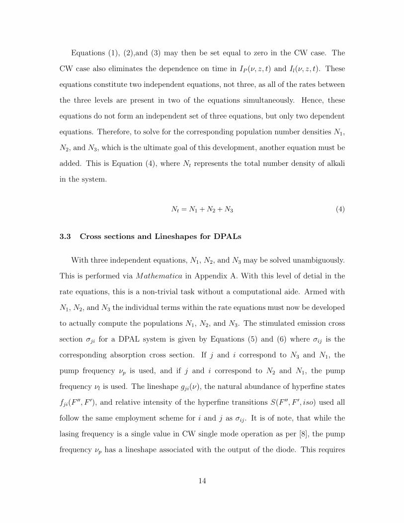
Equations (1), (2),and (3) may then be set equal to zero in the CW case. The
CW case also eliminates the dependence on time in IP (ν, z, t) and Il(ν, z, t). These
equations constitute two independent equations, not three, as all of the rates between
the three levels are present in two of the equations simultaneously. Hence, these
equations do not form an independent set of three equations, but only two dependent
equations. Therefore, to solve for the corresponding population number densities N1,
N2, and N3, which is the ultimate goal of this development, another equation must be
added. This is Equation (4), where Nt represents the total number density of alkali
in the system.
Nt = N1 +N2 +N3 (4)
3.3 Cross sections and Lineshapes for DPALs
With three independent equations, N1, N2, and N3 may be solved unambiguously.
This is performed via Mathematica in Appendix A. With this level of detial in the
rate equations, this is a non-trivial task without a computational aide. Armed with
N1, N2, and N3 the individual terms within the rate equations must now be developed
to actually compute the populations N1, N2, and N3. The stimulated emission cross
section σji for a DPAL system is given by Equations (5) and (6) where σij is the
corresponding absorption cross section. If j and i correspond to N3 and N1, the
pump frequency νp is used, and if j and i correspond to N2 and N1, the pump
frequency νl is used. The lineshape gji(ν), the natural abundance of hyperfine states
fji(F′′, F ′), and relative intensity of the hyperfine transitions S(F ′′, F ′, iso) used all
follow the same employment scheme for i and j as σij. It is of note, that while the
lasing frequency is a single value in CW single mode operation as per [8], the pump
frequency νp has a lineshape associated with the output of the diode. This requires
14
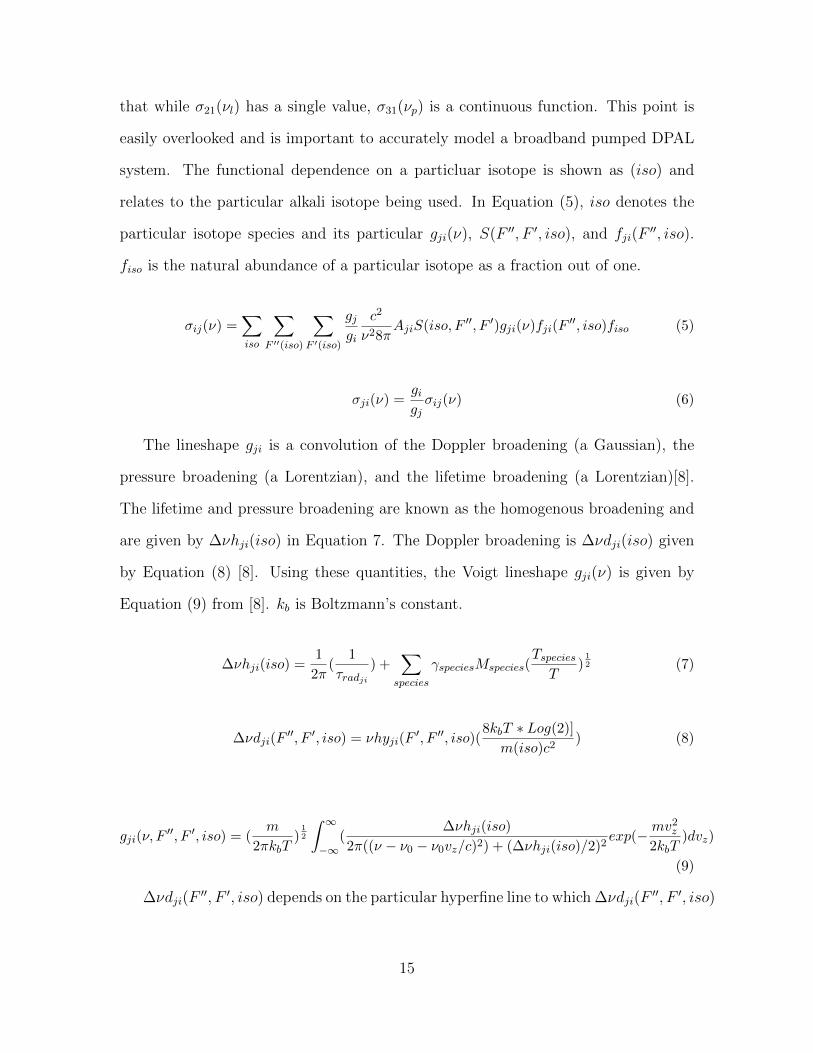
that while σ21(νl) has a single value, σ31(νp) is a continuous function. This point is
easily overlooked and is important to accurately model a broadband pumped DPAL
system. The functional dependence on a particluar isotope is shown as (iso) and
relates to the particular alkali isotope being used. In Equation (5), iso denotes the
particular isotope species and its particular gji(ν), S(F ′′, F ′, iso), and fji(F′′, iso).
fiso is the natural abundance of a particular isotope as a fraction out of one.
σij(ν) =∑iso
∑F ′′(iso)
∑F ′(iso)
gjgi
c2
ν28πAjiS(iso, F ′′, F ′)gji(ν)fji(F
′′, iso)fiso (5)
σji(ν) =gigjσij(ν) (6)
The lineshape gji is a convolution of the Doppler broadening (a Gaussian), the
pressure broadening (a Lorentzian), and the lifetime broadening (a Lorentzian)[8].
The lifetime and pressure broadening are known as the homogenous broadening and
are given by ∆νhji(iso) in Equation 7. The Doppler broadening is ∆νdji(iso) given
by Equation (8) [8]. Using these quantities, the Voigt lineshape gji(ν) is given by
Equation (9) from [8]. kb is Boltzmann’s constant.
∆νhji(iso) =1
2π(
1
τradji) +
∑species
γspeciesMspecies(TspeciesT
)12 (7)
∆νdji(F′′, F ′, iso) = νhyji(F
′, F ′′, iso)(8kbT ∗ Log(2)]
m(iso)c2) (8)
gji(ν, F′′, F ′, iso) = (
m
2πkbT)12
∫ ∞−∞
(∆νhji(iso)
2π((ν − ν0 − ν0vz/c)2) + (∆νhji(iso)/2)2exp(−mv
2z
2kbT)dvz)
(9)
∆νdji(F′′, F ′, iso) depends on the particular hyperfine line to which ∆νdji(F
′′, F ′, iso)
15

corresponds as each hyperfine transition has its own associate FWHM. The FWHM
depends upon F ′′, the original transition state in either N1, N2, or N3, and F ′, the
final state in N1, N2, or N3 [5]. Note, νhyji(F′, F ′′, iso) is the hyperfine frequency,
in Hz, for a transition from one state to another for a particular F ′, F ′′, and iso-
tope. νhyji(F′, F ′′, iso) is not the splitting between hyperfine levels within a single
fine level. That is νhysplitj(F′′, iso). Figures 2, 3, 4, 5, 6, and 7 show the transitions
between each of the hyperfine states of the D1 and D2 transitions for Cs, 85Rb, and
87Rb. The selection rule for F ′′ to F ′ is ∆F= +1,−1, or 0 with F ′′ = 0 to F ′ = 0
being forbidden. Figures 2, 3, 4, 5, 6, and 7 are taken from [5].
In practice, Equation (9) is difficult to use. An approximation using an error
function can be made as is employed as per [7]. The intermediate quantities given by
Equations (10), (11), and (12) are developed in this process. In Equation (12), the i
in front of uji(ν, F′′, F ′, iso) is the square root of negative one. For the remainder of
this thesis, Equation (13) will be used for gji(ν, F′′, F ′, iso), not Equation (9).
aji(ν, F′′, F ′, iso) = Log(2)
12
∆νhji(iso)
∆νdji(iso)(10)
uji(ν, F′′, F ′, iso) = 2Log(2)
12
(ν − νhyji(F ′′, F ′, iso))∆νdji(F ′′, F ′, iso)
(11)
zji(ν, F′′, F ′, iso) = aji(ν, F
′′, F ′, iso) + ı ∗ uji(ν, F ′′, F ′, iso) (12)
gji(ν, F′′, F ′, iso) =
4Log(2)
π
1/2 1
∆νdji(F ′′, F ′, iso)Re(ezji(ν,F
′′,F ′,iso)2Erfc(zji(ν, F′′, F ′, iso)))
(13)
To calculate the lineshape, the relative strength S(species, F ′′, F ′, iso) of a tran-
sition between hyperfine levels must be known [5]. The relative intensities of each of
16

Figure 2. The D1 manifold for 133Cs without possible transitions listed. The frequencyspacing of each hyperfine state is listed [5].
17

Figure 3. The D2 manifold for 133Cs without possible transitions listed. The frequencyspacing of each hyperfine state is listed [5].
18

Figure 4. The D1 manifold for 85Rb without possible transitions listed. The frequencyspacing of each hyperfine state is listed [5].
19

Figure 5. The D2 manifold for 85Rb without possible transitions listed. The frequencyspacing of each hyperfine state is listed [5].
20
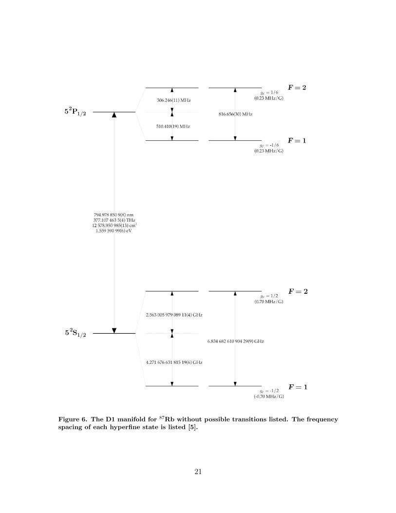
Figure 6. The D1 manifold for 87Rb without possible transitions listed. The frequencyspacing of each hyperfine state is listed [5].
21

Figure 7. The D2 manifold for 87Rb without possible transitions listed. The frequencyspacing of each hyperfine state is listed [5].
22

the transitions for the D1 and D2 transitions may be found in Tables 1, 2, and 3.
The data in Tables 1, 2, and 3 comes from [5].
The relative natural abundance of each hyperfine state as a fraction of one is
fji(F′′, iso). fji(F
′′, iso) is given by Equation (14). The relative natural abundance
is the fraction of atoms in each of the initial hyperfine states F ′′. It is of note that
νhysplitj(F′′, iso) is not equal to νhyji(F
′′, F ′, iso). νhysplitj(F′′, iso) is the frequency in
Hz of the splitting between a particular hyperfine level and the center frequency of
the fine structure level which the hyperfine level is in. While, νhyji(F′′, F ′, iso) is the
frequency in Hz of a F ′′ → F ′ hyperfine transition between two fine structure levels.
Simply put, νhysplitj(F′′, iso) is an energy splitting in Hz given on Figures 2, 3, 4, 5,
6, and 7 and νhyji(F′′, F ′, iso) is the absolute difference between two hyperfine levels
in different fine structure levels.
fji(F′′, iso) =
(2F ′′ + 1)exp(h(νji−νhysplitj (F
′′,iso))
kbT)∑
iso
∑F ′′
(2F ′′ + 1)exp(hνhysplitj (F
′′,iso)
kbT)
(14)
3.4 Alkali and Collision Partner Properties
Several other important material quantities are needed to calculate Equation (6).
Table 4 provides these quantities for Cs and Rb.
From the numbers in Table 4 and using equations from [8], several more needed
quantities are developed. These include Bji and kji.
Bji(ν, iso) =c3Aji(iso)
n38πhν3(15)
Bij(ν, iso) =gjgiBji(ν, iso) (16)
23

Table 1. S(species, F ′′, F ′, iso) for 133Cs for Hyperfine Structure
D1 Manifold D2 ManifoldF ′′ → F ′ or 2S 1
2→ 2P 1
2S(species, F ′′, F ′, iso) F ′′ → F ′ or 2P 1
2→ 2P 3
2S(species, F ′′, F ′, iso)
3→ 3 1/4 3→ 2 5/143→ 4 3/4 3→ 3 3/84→ 3 7/12 3→ 4 15/564→ 4 5/12 4→ 3 7/72
- - 4→ 4 7/24- - 4→ 5 7/18
Table 2. S(species, F ′′, F ′, iso) for 85Rb for Hyperfine Structure
D1 Manifold D2 ManifoldF ′′ → F ′ or 2S 1
2→ 2P 1
2S(species, F ′′, F ′, iso) F ′′ → F ′ or 2P 1
2→ 2P 3
2S(species, F ′′, F ′, iso)
2→ 2 2/9 2→ 1 3/102→ 3 7/9 2→ 2 7/183→ 2 5/9 2→ 3 14/453→ 3 4/9 3→ 2 5/63
- - 3→ 3 5/18- - 3→ 4 9/14
Table 3. S(species, F ′′, F ′, iso) for 87Rb for Hyperfine Structure
D1 Manifold D2 ManifoldF ′′ → F ′ or 2S 1
2→ 2P 1
2S(species, F ′′, F ′, iso) F ′′ → F ′ or 2P 1
2→ 2P 3
2S(species, F ′′, F ′, iso)
1→ 1 1/6 1→ 0 1/61→ 2 5/6 1→ 1 5/122→ 1 1/2 1→ 2 5/122→ 2 1/2 2→ 1 1/20
- - 2→ 2 1/4- - 2→ 3 7/10
24
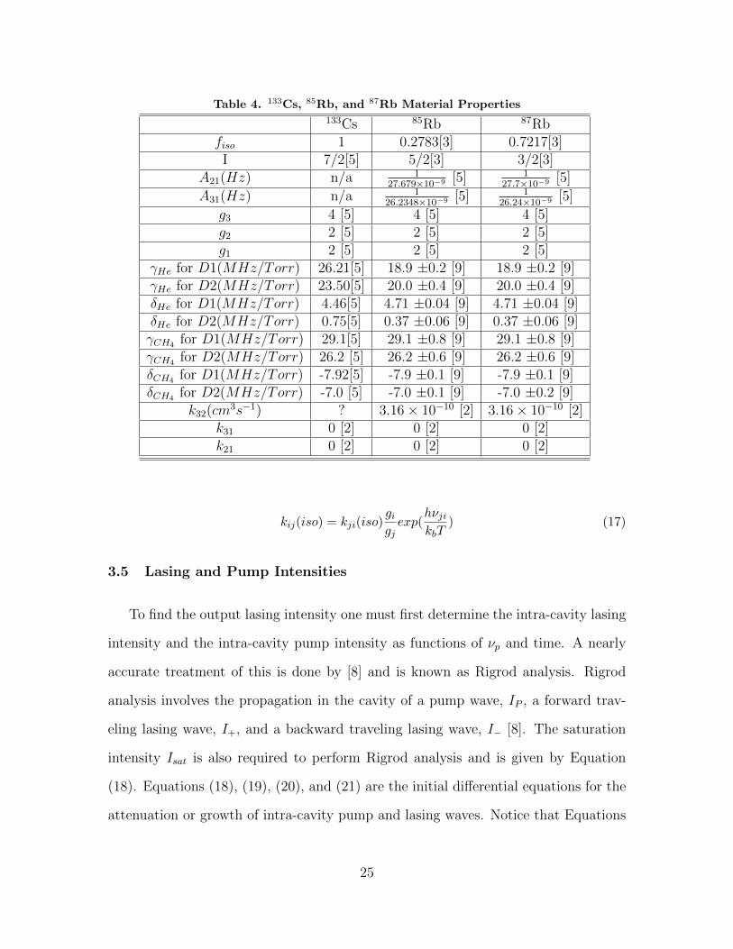
Table 4. 133Cs, 85Rb, and 87Rb Material Properties
133Cs 85Rb 87Rbfiso 1 0.2783[3] 0.7217[3]I 7/2[5] 5/2[3] 3/2[3]
A21(Hz) n/a 127.679×10⁻⁹ [5] 1
27.7×10⁻⁹ [5]
A31(Hz) n/a 126.2348×10⁻⁹ [5] 1
26.24×10⁻⁹ [5]
g3 4 [5] 4 [5] 4 [5]g2 2 [5] 2 [5] 2 [5]g1 2 [5] 2 [5] 2 [5]
γHe for D1(MHz/Torr) 26.21[5] 18.9 ±0.2 [9] 18.9 ±0.2 [9]γHe for D2(MHz/Torr) 23.50[5] 20.0 ±0.4 [9] 20.0 ±0.4 [9]δHe for D1(MHz/Torr) 4.46[5] 4.71 ±0.04 [9] 4.71 ±0.04 [9]δHe for D2(MHz/Torr) 0.75[5] 0.37 ±0.06 [9] 0.37 ±0.06 [9]γCH4 for D1(MHz/Torr) 29.1[5] 29.1 ±0.8 [9] 29.1 ±0.8 [9]γCH4 for D2(MHz/Torr) 26.2 [5] 26.2 ±0.6 [9] 26.2 ±0.6 [9]δCH4 for D1(MHz/Torr) -7.92[5] -7.9 ±0.1 [9] -7.9 ±0.1 [9]δCH4 for D2(MHz/Torr) -7.0 [5] -7.0 ±0.1 [9] -7.0 ±0.2 [9]
k32(cm3s−1) ? 3.16× 10⁻¹⁰ [2] 3.16× 10⁻¹⁰ [2]
k31 0 [2] 0 [2] 0 [2]k21 0 [2] 0 [2] 0 [2]
kij(iso) = kji(iso)gigjexp(
hνjikbT
) (17)
3.5 Lasing and Pump Intensities
To find the output lasing intensity one must first determine the intra-cavity lasing
intensity and the intra-cavity pump intensity as functions of νp and time. A nearly
accurate treatment of this is done by [8] and is known as Rigrod analysis. Rigrod
analysis involves the propagation in the cavity of a pump wave, IP , a forward trav-
eling lasing wave, I+, and a backward traveling lasing wave, I− [8]. The saturation
intensity Isat is also required to perform Rigrod analysis and is given by Equation
(18). Equations (18), (19), (20), and (21) are the initial differential equations for the
attenuation or growth of intra-cavity pump and lasing waves. Notice that Equations
25

(19), (20), and (21) are transcendental. Also, remember that N1, N2, and N3 depend
on IP , I+, and I−. This dependence is extremely lengthy and is shown in Appendix
A. These two facts greatly increase the solution difficulty of these differential equa-
tions. Equations (19), (20), and (21) require numerical differential equation solution
techniques to solve. Equations (20) and (21) appear without the terms which go as
the inverse of I+ plus I− divided by Isat because the population densities (N1, N2,
and N3) maintain their dependence on IP , I+, and I− [8].
Isat(νp) =hνp
σ31(νp)
∑iso
(1
τrad(iso)fiso) (18)
dIP (z, νl, νp)
dz= σ31(νp)[N3(z, νl, νp)−
g3g1N1(z, νl, νp)]IP (z, νl, νp) (19)
dI+(z, νl, νp)
dz= σ21(νl)[N2(z, νl, νp)−
g2g1N1(z, νl, νp)]I+(z, νl, νp) (20)
dI−(z, νl, νp)
dz= −σ21(νl)[N2(z, νl, νp)−
g2g1N1(z, νl, νp)]I+(z, νl, νp) (21)
The crux of the simulation lies in solving Equations (19), (20), and (21). The
solution to these differential equations requires three boundary conditions. Initial
conditions are not used as the solution is time-independent for the CW case. Equa-
tions (22), (23), and (24) provide these boundary conditions as given by [8] for Rigrod
analysis, where νd is the line center of the diode’s spectral profile in Hz. z0 is the po-
sition of the beginning of the gain cell and zf is the position of the end of the gain cell.
Note, that z denotes the functional dependence of an equation upon longitundinal
position in m in the alkali gain cell.
IP (z0, νl, νp) = IP 0g31(νp)
g31(νd)(22)
26
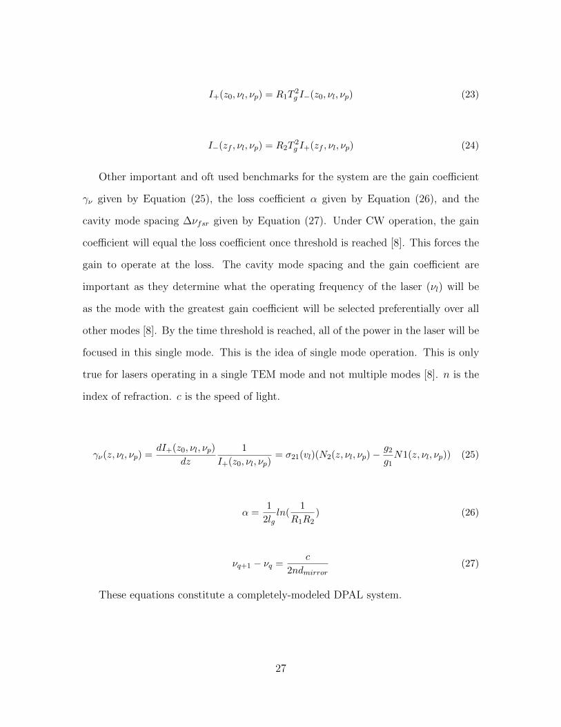
I+(z0, νl, νp) = R1T2g I−(z0, νl, νp) (23)
I−(zf , νl, νp) = R2T2g I+(zf , νl, νp) (24)
Other important and oft used benchmarks for the system are the gain coefficient
γν given by Equation (25), the loss coefficient α given by Equation (26), and the
cavity mode spacing ∆νfsr given by Equation (27). Under CW operation, the gain
coefficient will equal the loss coefficient once threshold is reached [8]. This forces the
gain to operate at the loss. The cavity mode spacing and the gain coefficient are
important as they determine what the operating frequency of the laser (νl) will be
as the mode with the greatest gain coefficient will be selected preferentially over all
other modes [8]. By the time threshold is reached, all of the power in the laser will be
focused in this single mode. This is the idea of single mode operation. This is only
true for lasers operating in a single TEM mode and not multiple modes [8]. n is the
index of refraction. c is the speed of light.
γν(z, νl, νp) =dI+(z0, νl, νp)
dz
1
I+(z0, νl, νp)= σ21(vl)(N2(z, νl, νp)−
g2g1N1(z, νl, νp)) (25)
α =1
2lgln(
1
R1R2) (26)
νq+1 − νq =c
2ndmirror(27)
These equations constitute a completely-modeled DPAL system.
27

IV. Simulation Description
4.1 Overview
The simulation of the model developed in Chapter III is performed in Mathematica
7.0 for Windows XP on a 2.0 GHz AMD processor. The simulation reads in a list of
input parameters, then uses all of the equations developed in Chapter III to simulate
a DPAL system. Then using the differential equation solving, data analysis, and visu-
alizations packages in Mathematica the system is characterized as detailed in Chap-
ter III. The outputs required of the system are Ip(z, νl, νp), I+(z, νl, νp), I−(z, νl, νp),
γν(z, νl, νp), α, N1(z, νl, νp), N2(z, νl, νp), N3(z, νl, νp), and the output laser intensity,
Iout, which is the output at the single laser frequency, νl
4.2 Assumptions
Without simplifying assumptions simulating the DPAL model discussed in Chap-
ter III would not be practical as a single threaded process on a desktop computer.
Assumptions were made to simplify the problem, but these assumptions were chosen
such that a high degree of fidelity is maintained in the simulation’s outputs. The
DPAL system is assumed to be CW in its pump and response. Hence, all time depen-
dence is eliminated. For any system which runs for longer than approximately one
ms this is an adequate assumption because the population densities will reach their
equilibrium values within that time. Only transitions within the three level system
shown in Figure 1 are assumed to occur. All other transitions within the alkali atom
are ignored. This assumption is somewhat valid as the absorption and emission cross
section for the 2S 12→ 2P 3
2and 2P 1
2→ 2S 1
2are much larger (approximately 104 times
larger) than any of the other transitions.
It is assumed that no forbidden hyperfine transitions occur within or between the
28

sublevels. The effects of the hyperfine structure beyond its effects on the lineshape
gji(ν) are neglected. The hyperfine structure in a physical system does play a part in
the rate between each sublevel. Hence, a fully complete model would need to create
rate equations, such as Equations (1),(2), and (3), for each possible (including the
forbidden transitions) hyperfine transition. The populations of each hyperfine level
would also have to be independent of one another. Transitions between hyperfine
levels due to collisions, absorption, and emission would also have to be tracked. Fur-
ther, the lasing intensity would not be single quantity but a set of intensities each
associated with a transition on the D1 manifold. Each intensity would require an in-
dividual plus wave and minus wave differential equation like Equations (20) and (21).
Thus, the system would contain not three coupled non-linear ODEs, but instead 13.
Also, the collisional excitation and de-excitation rates between hyperfine levels are
unknown. Adding this complexity to the model is both extremely complicated and
computationally difficult without the use of multi-threading. The laser modeled is as-
sumed to operate only in the TEM(0,0) mode and to not operate in any other modes.
The mode volume is assumed to be completely filled. The energy lost because of
unfilled mode volume is not considered. This assumption is only somewhat valid, but
it is difficult to simulate the effects of partially filling the mode volume of a DPAL
because these effects are not yet fully characterized in the literature.
4.3 Simulation Input Parameters
The inputs to the simulation are listed in Table 5. Each parameter is given with
its normal range of values. The input parameters are not physical constants, but
are rather variables which are dynamic between different DPAL systems. Collisional
relaxation rate coefficients such as k32 are not considered input parameters. These
are considered physical constants of the system and are not input by the user. The
29
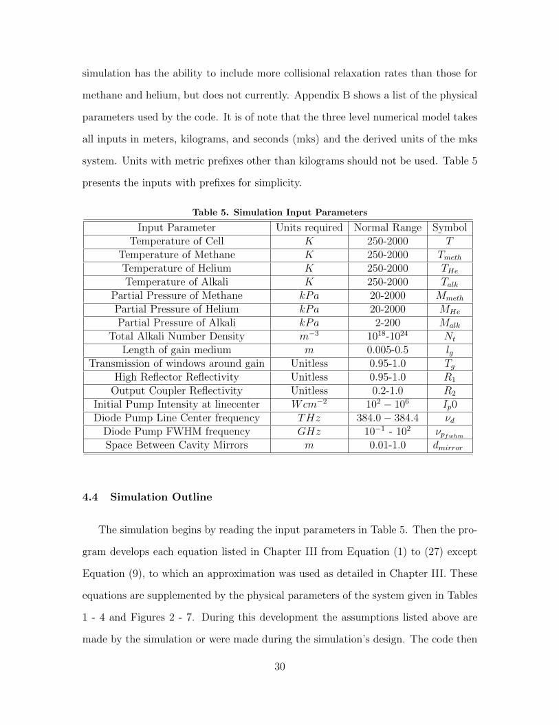
simulation has the ability to include more collisional relaxation rates than those for
methane and helium, but does not currently. Appendix B shows a list of the physical
parameters used by the code. It is of note that the three level numerical model takes
all inputs in meters, kilograms, and seconds (mks) and the derived units of the mks
system. Units with metric prefixes other than kilograms should not be used. Table 5
presents the inputs with prefixes for simplicity.
Table 5. Simulation Input Parameters
Input Parameter Units required Normal Range SymbolTemperature of Cell K 250-2000 T
Temperature of Methane K 250-2000 TmethTemperature of Helium K 250-2000 THeTemperature of Alkali K 250-2000 Talk
Partial Pressure of Methane kPa 20-2000 Mmeth
Partial Pressure of Helium kPa 20-2000 MHe
Partial Pressure of Alkali kPa 2-200 Malk
Total Alkali Number Density m−3 1018-1024 Nt
Length of gain medium m 0.005-0.5 lgTransmission of windows around gain Unitless 0.95-1.0 Tg
High Reflector Reflectivity Unitless 0.95-1.0 R1
Output Coupler Reflectivity Unitless 0.2-1.0 R2
Initial Pump Intensity at linecenter Wcm−2 102 − 106 Ip0Diode Pump Line Center frequency THz 384.0− 384.4 νd
Diode Pump FWHM frequency GHz 10−1 - 102 νpfwhm
Space Between Cavity Mirrors m 0.01-1.0 dmirror
4.4 Simulation Outline
The simulation begins by reading the input parameters in Table 5. Then the pro-
gram develops each equation listed in Chapter III from Equation (1) to (27) except
Equation (9), to which an approximation was used as detailed in Chapter III. These
equations are supplemented by the physical parameters of the system given in Tables
1 - 4 and Figures 2 - 7. During this development the assumptions listed above are
made by the simulation or were made during the simulation’s design. The code then
30

constitutes a fully-developed model of a DPAL system. If the differntial equations
(19), (20), and (21) can be solved numerically for this system, then all of the pa-
rameters needed to characterize the system can be developed from that solution. In
practice, the solution of Equations (19), (20), and (21) is difficult and requires the
use of Mathematica’s innate numerical differential equation solver. The differential
equation solver is utilized with a shooting method and the boundary conditions of
Equations (22), (23), and (24). To solve Equations (19), (20), and (21) requires that
a shooting method be performed for different initial values for I+ and I− at z0. Each
shot is then solved by the numerical differential equation solver for a solution to the
differential equations in z or position. An algorithm then assigns the best starting I+
and I− values based upon the occurrence of gain above loss and on the degree of ad-
herence to Equation (24). This solution architecture is then utilized for a select set of
pump frequencies spanning three times the pump’s full width at half max (FWHM).
The solutions which best match the boundary condition for each discrete pump fre-
quency are then interpolated between by Mathematica’s data analysis software and
are plotted. This architecture is detailed in Figure 8. The complete Mathematica
notebook can be found in Appendix B.
4.5 Simulation Outputs
The outputs of the simulation are the way in which the model is both com-
pared to other models such as [2],[3], and [5], and then, the outputs are compared
to experimental results. To achieve these comparisons several different outputs are
provided. A profile of the pump intensity IP (z, νp) is shown throughout the entire
cell. I+(z, νp, νl) and I−(z, νp, νl) are plotted. The population densities, N1(z, νp),
N2(z, νp), and N3(z, νp) are plotted. The output lasing intensity (Iout) is determined.
The simulation selects the lasing mode with the greatest gain and outputs its fre-
31

Figure 8. The architecture used to develop the simulation of the DPAL model. Oc-tagons are output plots or printed output system characteristics. Rectangles are algo-rithms.
32

quency, as this is the frequency of the laser’s output. γν(z) is plotted for the system.
The average value of γν over z is compared to α and should be found to be roughly
equivalent. A determination of the degree to which the chosen solution matches the
boundary conditions is provided.
33

V. Results and Simulation Comparisons
5.1 Chapter Overview
To validate the model this thesis develops, which is henceforth known as the three
level numerical model; it must be tested against similar previously vetted systems
like the Lewis model and the Hager model. If the outputs of the model developed are
comparable to those developed by Lewis and Hager in the regime where those models
are known to operate well, then the model’s output outside of those regimes is more
believable. The model will also be tested against experimental results. Further,
the model will be shown to simulate a DPAL with an extremely high initial pump
intensity and other features typically found only during pulsed operation. The model
will also perform Rigord analysis for a general DPAL case. Together these outputs
will show the effectiveness and utility of the model and its simulation.
5.2 Comparison to Lewis Model
5.2.1 Inputs.
The inputs of Table 6 are derived from the DPAL quasi two level regime of Lewis’s
thesis [5]. The inputs are listed in the units used by Lewis in [5] rather than units used
by the three level numerical model. If an input was not listed by Lewis, a suitable
value was devised. This applies specifically to the temperature of the alkali for plots
provided in [5]. The alkali used for this comparison was Rb, which is used throughout
the comparison between the three level numerical model and the Lewis model. These
inputs will be used throughout the comparison to Lewis’s model and the three level
numerical model for the remainder of this section unless otherwise noted. Lewis lists
one of his buffer gases as ethane in [5]. However, his theortical development and plots
list methane as the buffer gas used. Further [5] lists methane, not ethane, as his
34
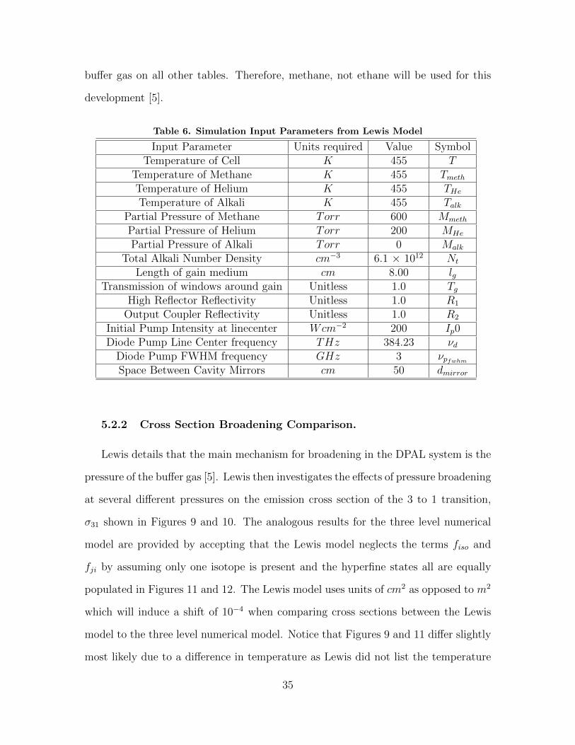
buffer gas on all other tables. Therefore, methane, not ethane will be used for this
development [5].
Table 6. Simulation Input Parameters from Lewis Model
Input Parameter Units required Value SymbolTemperature of Cell K 455 T
Temperature of Methane K 455 TmethTemperature of Helium K 455 THeTemperature of Alkali K 455 Talk
Partial Pressure of Methane Torr 600 Mmeth
Partial Pressure of Helium Torr 200 MHe
Partial Pressure of Alkali Torr 0 Malk
Total Alkali Number Density cm−3 6.1 × 10¹² Nt
Length of gain medium cm 8.00 lgTransmission of windows around gain Unitless 1.0 Tg
High Reflector Reflectivity Unitless 1.0 R1
Output Coupler Reflectivity Unitless 1.0 R2
Initial Pump Intensity at linecenter Wcm−2 200 Ip0Diode Pump Line Center frequency THz 384.23 νd
Diode Pump FWHM frequency GHz 3 νpfwhm
Space Between Cavity Mirrors cm 50 dmirror
5.2.2 Cross Section Broadening Comparison.
Lewis details that the main mechanism for broadening in the DPAL system is the
pressure of the buffer gas [5]. Lewis then investigates the effects of pressure broadening
at several different pressures on the emission cross section of the 3 to 1 transition,
σ31 shown in Figures 9 and 10. The analogous results for the three level numerical
model are provided by accepting that the Lewis model neglects the terms fiso and
fji by assuming only one isotope is present and the hyperfine states all are equally
populated in Figures 11 and 12. The Lewis model uses units of cm2 as opposed to m2
which will induce a shift of 10−4 when comparing cross sections between the Lewis
model to the three level numerical model. Notice that Figures 9 and 11 differ slightly
most likely due to a difference in temperature as Lewis did not list the temperature
35

he used to create Figure 9. Figures 10 and 12 are identical. This implies that the
lineshapes and cross sections developed by the three level numerical model agree well
with those of the Lewis model especially at high pressures. Note Figures 9, 10, 11,
and 12 are all offset in frequency space by ν31.
Figure 9. σ31 for 100 Torr helium and 100 Torr methane from the Lewis model [5]
5.2.3 Absorption Profile Comparison.
The absorption profiles for the DPAL regime from the Lewis model are given by
Figure 13 from [5]. The same inputs were provided to the three level numerical model
and the comparable output is given by Figure 14. Notice that the frequency axis in
Figure 13 is offset based on pump line center frequency νd, the intensity is in Wcm−2,
and the position within the gain medium (z) is in cm. Figure 13’s units are based
on the MKS system. Figure 14 shows similar features to Figure 13, however, small
changes from the more complete rate equation analysis and the use of the terms fiso
and fji are noticeable at the far end of the cell. Hence, the Lewis model captures a
36

Figure 10. σ31 for 1000 Torr helium and 1000 Torr methane from the Lewis model [5]
Figure 11. σ31 for 100 Torr helium and 100 Torr methane from the three level numericalmodel
37

Figure 12. σ31 for 1000 Torr helium and 1000 Torr methane from the three levelnumerical model
great deal of the absorption effects within the gain medium, but it does not develop
a wholly accurate picture of the attenuation of the pump wave.
The Lewis model also develops the attenuation of the pump intensity under the
quasi-two level approach (QTLA), and based upon the QTLA assumption, is able
to develop the amount of attenuation of the pump intensity due to lasing. This
development is somewhat ad− hoc, and will not work properly at threshold and will
not give a spectral profile for the occurrence of lasing. That is, the pump is assumed
to cause lasing to occur and then will be attenuated to a greater degree based upon
an assumed lasing intensity which will occur over all pump frequencies to an equal
degree. This effect can be seen in Figure 15 with the inputs of Table 6. In actuality
only those pump photons which cause lasing to occur in the gain medium will see
this effect. Hence, only certain pump frequencies will exhibit this effect; those that
induce lasing to occur. Those pump frequencies which do not provide enough energy
38

Figure 13. The Lewis model 3D absorption profile without lasing for inputs of Table6. Note the units of the plot are not MKS and the frequency is offset by νd [5].
39
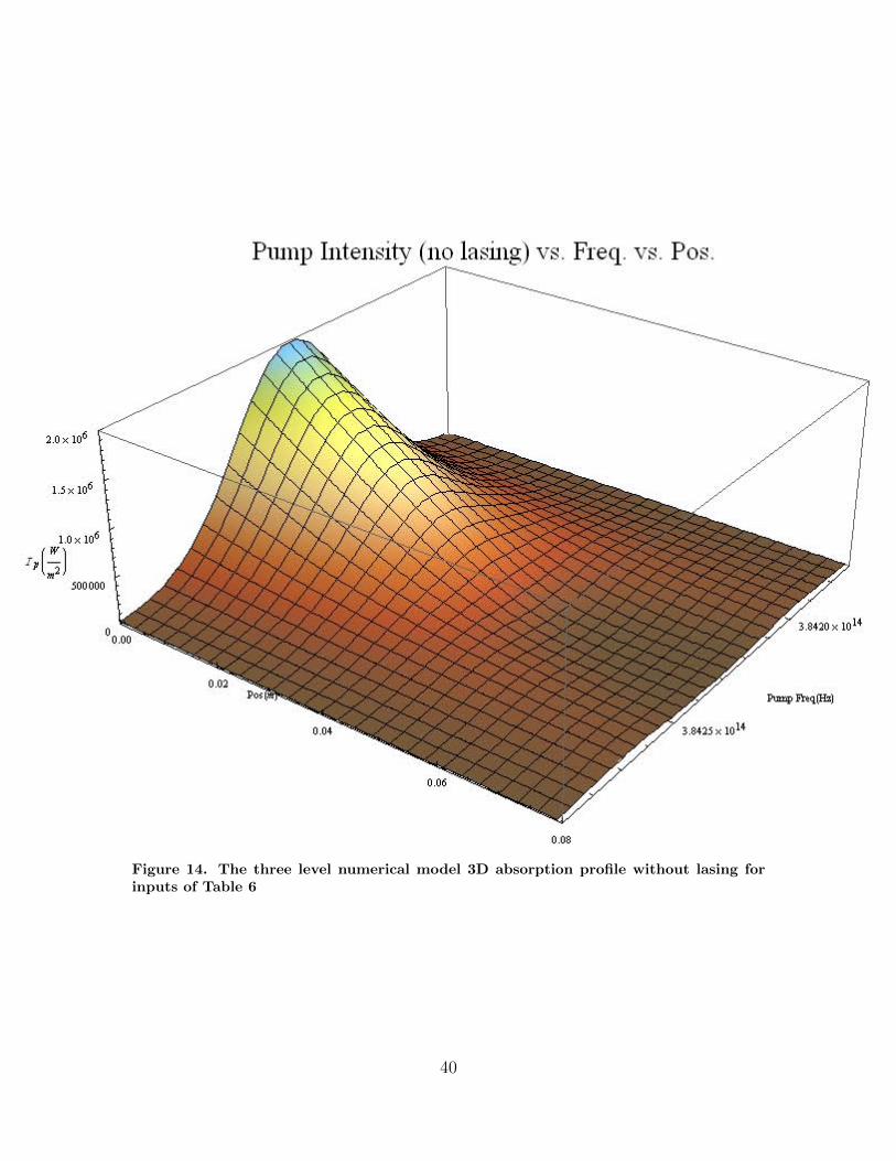
Figure 14. The three level numerical model 3D absorption profile without lasing forinputs of Table 6
40
to maintain gain above loss will not observe this effect. This can be seen in Figure
16, created with the inputs of Table 6 by the three level numerical model. Lasing
is observed to occur in the frequency domain between the two peak features which
propagate through to the end of the cell. Also, note that it appears that the pump
intensity in the area without lasing has grown between Figures 14 and 16. This
is simply an optical illusion due to the degree to which a discontinuity appears in
frequency space due to achieving threshold inversion. A close inspection of Figures
14 and 16 will reveal this fact. By comparing Figures 15 and 16, one can see that the
Lewis model is able to only approximate the effect of the attenuation of the pump due
to intra-cavity lasing. This effect is negligible well above threshold (30 times Isat).
The three level numerical model also simulated γ(z) for the lasing region of Figure
16 given in Figure 17. Figure 17 only shows the area with positive gain. An effective
laser should end when gain dips below zero as the intra-cavity lasing waves will be
absorbed beyond this point.
5.3 Comparison to Hager Model
5.3.1 Spectral Profile Comparison.
In [3], Hager develops a spectral line profile of the absorption of the D1 transition
for all hyperfine states of Rb. The data Hager presents is based upon experimental
data and is then fit to his development of the Voigt profile. The absorption profile
calculated by Hager is given in Figure 18. The analogous emission spectra is provided
for the three level numerical model in Figure 19. Figure 18’s absorption features are
shown to be exactly mirrored in the emission profile given by Figure 19. Thus, the
three level model is able to fit both experimental lineshape data and the Hager model
lineshape for a spectra including all of the naturally occurring isotopes of Rb and all
of the hyperfine transitions of the D1 manifold.
41

Figure 15. The Lewis model 3D absorption profile with QTLA lasing inputs of Table6. Note the units of the plot are not MKS and the frequency is offset by νd [5].
42

Figure 16. The three level numerical model 3D absorption profile with lasing for inputsof Table 6. Lasing is only occurring, in frequency space, in the region between the twopeak features which propagate throughout the cell.
43

Figure 17. The three level numerical model determination of γ(z) for inputs of Table 6within the lasing region. Notice that the gain is only provided while γ is above zero.
44

Figure 18. The hyperfine absorption profile for the Rb. D1 manifold offset by ν21 [3]
Figure 19. The three level numerical model lineshape for the Rb. D1 manifold offsetby ν21
45

5.4 CW Simulation of a Pulsed System
Pulsed DPAL systems typically operate at extremely high intensities compared to
CW systems, however, as long as the population densities reach their equilibrium val-
ues a CW simulation is apt for a pulsed system. Even in systems which do not achieve
equilibrium, the rate equations for the population concentrations remain unchanged
from Chapter II. So, if the rate at which populations change with time is small with
respect to the time scale of the pulse width of the diode and the populations are
assumed to reach semi-equilibrium quickly after interaction with the pulse, then, this
development is still at least somewhat valid. Hence, the three level numerical model
can be applied to high intensity systems and may be used to give rough estimates of
the characteristics of some pulsed DPAL systems. Typical inputs for the operation
of a pulsed DPAL system can be found in Table 7.
Table 7. Simulation Input Parameters for CW Simulation of a Pulsed System
Input Parameter Units required Value SymbolTemperature of Cell K 500 T
Temperature of Methane K 500 TmethTemperature of Helium K 500 THeTemperature of Alkali K 500 Talk
Partial Pressure of Methane Torr 1000 Mmeth
Partial Pressure of Helium Torr 1000 MHe
Partial Pressure of Alkali Torr 0 Malk
Total Alkali Number Density m−3 3.79 × 10¹⁹ Nt
Length of gain medium m 0.01 lgTransmission of windows around gain Unitless 1.0 Tg
High Reflector Reflectivity Unitless 1.0 R1
Output Coupler Reflectivity Unitless 0.5 R2
Initial Pump Intensity GWm−2 5 Ip0Diode Pump Line Center frequency THz 384.23 νd
Diode Pump FWHM frequency GHz 50 νpfwhm
Space Between Cavity Mirrors m 0.1 dmirror
The outputs of the three level numerical model for the inputs of Table 7 are
46
given in Figures 20 - 23 and Table 8. Figure 20 provides the degree to which the
diode pump lineshape was matched with the lineshape of the alkali atom. In this
case, the areas overlap about 80 percent. In general, the pump lineshape should be
well matched to the transition it is attempting to pump, otherwise energy will be
lost. Based on Figure 21 most of the pump’s input intensity is still present at the
output coupler, implying that the gain cell should be extended if possible. Unlike in
Figure 16, the pump intensity in Figure 21 is not observed to have a region which
is being attenuated by laser operation and a region which is not. This is due to
lasing occurring across the entire pump spectrum provided in Figure 21. Figure 22
shows the gain as a function of z. The gain can be seen to decrease as the pump
attenuates. However, the gain does not decrease linearly with position, which implies
that approximations such as LAND may not be valid in this case. The total gain
in Table 8 is the average value of the gain in Figure 22. In Table 8 γ(total)/α is a
measure to how well the system followed the approximation that gain equals loss. At
infinite fidelity γ(total)/α should equal unity. So, γ(total)/α is a measure of merit
of how well the system performed. The average residual in solutions listed in Table
8 is the of average of all residuals of the routine which chose the best adherence to
the boundary condition at the output coupler, i.e. Equation (24). This average is
only computed for those cases in which lasing is determined by the simulation to be
occurring. Figure 23 shows the forward traveling wave (upper) and the backward
traveling wave (lower). Notice that difference between the upper wave and the lower
wave at the end of the cell is equal to the reflectivity of the output coupler times the
square of the transmissivity of the gain cell, which in this case is 0.5.
47

Figure 20. The lineshape g31 with the pump lineshape gp overlayed to show the degreeof area matching. Note the frequency is offset by νd [5].
Figure 21. The intensity of the pump (IP ) as it propagates through the cell
48

Figure 22. The gain γ as a function of z.
Figure 23. The Integrated Plus Wave Intensity(upper) and Minus Wave Inten-sity(lower) as functions of z. The output coupling is the space between the upperwave and lower wave at the edge of the graph.
49

Table 8. Simulation Outputs Characteristics for CW Simulation of a Pulsed System
Input Parameter Units Value SymbolOutput Laser Intensity MWm−2 63.7 Iout
Output Laser Frequency THz 377.107 νlIout/Ip Out of 1 0.128 n/aIp/Isat n/a 5002. n/a
γ(total)/α n/a 1.001 n/aAverage residual in solutions n/a 0.0094 n/a
5.5 Simulation of a System Near Threshold
One of the more difficult regimes to model in most cases is the regime at or near
threshold. The three level numerical model is able to simulate threshold systems
effectively. The inputs for three level numerical model for a threshold system are
given by Table 9. Under these conditions, only a the center bandwidth of the pump
wave can induce a population inversion, and thus lasing. This effect is visible in Figure
24. The outputs of the three level numerical model are provided in Table 10. Near
threshold the three level numerical model had difficulty obtaining an interpolation
for γ(total) so it is not listed. The difficulty seems to arise from the sharpness of the
gain profile for a threshold case.
50

Table 9. Simulation Input Parameters for a Threshold System
Input Parameter Units required Value SymbolTemperature of Cell K 450 T
Temperature of Methane K 450 TmethTemperature of Helium K 450 THeTemperature of Alkali K 450 Talk
Partial Pressure of Methane Torr 500 Mmeth
Partial Pressure of Helium Torr 500 MHe
Partial Pressure of Alkali Torr 0 Malk
Total Alkali Number Density m−3 6.1 × 10¹⁸ Nt
Length of gain medium m 0.02 lgTransmission of windows around gain Unitless 1.0 Tg
High Reflector Reflectivity Unitless 1.0 R1
Output Coupler Reflectivity Unitless 0.9999 R2
Initial Pump Intensity kWm−2 600 Ip0Diode Pump Line Center frequency THz 384.23 νd
Diode Pump FWHM frequency GHz 5 νpfwhm
Space Between Cavity Mirrors m 0.1 dmirror
Table 10. Simulation Outputs Characteristics for a Threshold System
Input Parameter Units Value SymbolOutput Laser Intensity Wm−2 11.2 Iout
Output Laser Frequency THz 377.109 νlIout/Ip Out of 1 0.000020 n/aIp/Isat n/a 1.25 n/a
γ(total)/α n/a n/a n/aAverage residual in solutions n/a 0.35 n/a
51
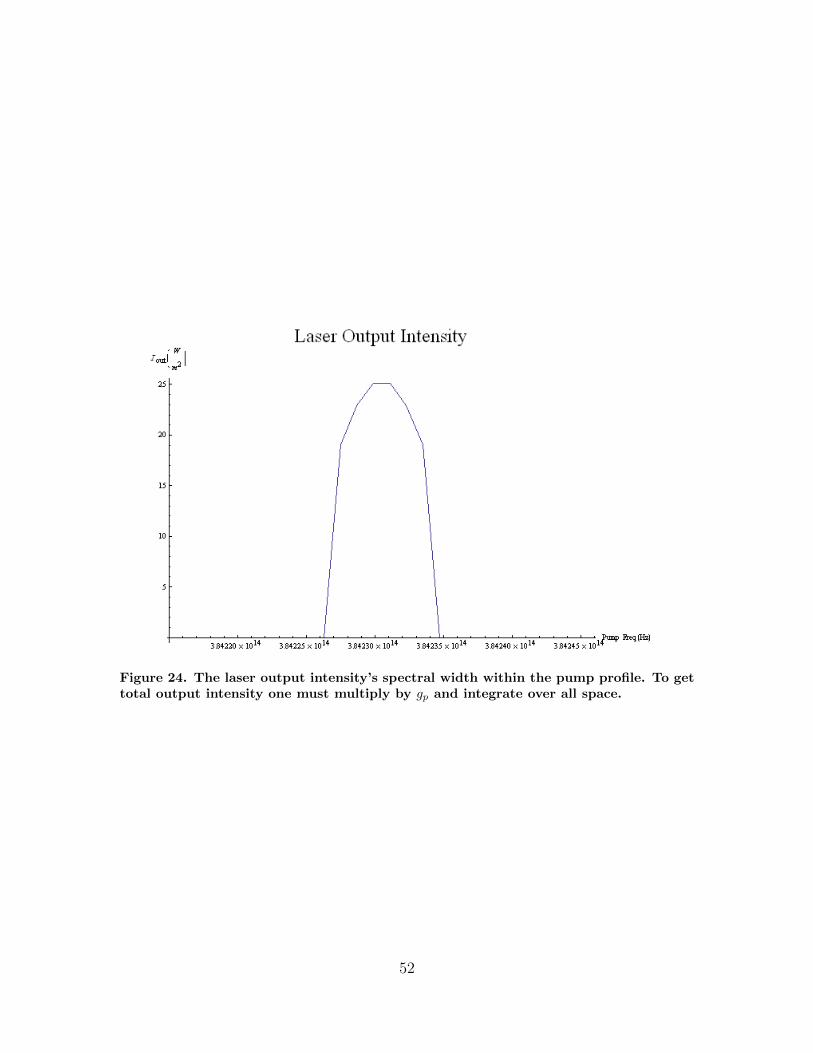
Figure 24. The laser output intensity’s spectral width within the pump profile. To gettotal output intensity one must multiply by gp and integrate over all space.
52

VI. Conclusions
6.1 Comparison to Other Models
The three level numerical model is able to replicate the results of both the Lewis
model and the Hager model and to produce expected results that neither of these
models are able to. The three level numerical model offers a much higher fidelity under
many circumstances, but with that added fidelity comes a much more cumbersome
development and a lack of intuitive understanding of the problem, which is a hallmark
of the Lewis and Hager models. Hence, the three level numerical model provides
another option for the simulation of DPAL systems, but does not supersede previous
developments.
6.2 Use as a Research Tool
Though the three level numerical model can be somewhat difficult to utilize and
to interpret, it provides a great deal of fidelity for research into many areas which no
other DPAL simulation can provide. The three level numerical model handles broad-
band pumping, produces a complete analysis of the rate equations for the three level
DPAL system, selects preferential gain from cavity mode spacing, develops the hy-
perfine lineshape for multiple isotopes, allows the use of multiple buffer gases, allows
for quenching to be simulated, and solves a set of three coupled non-linear transcen-
dental differential equations to characterize any three level CW DPAL system under
any regime to high fidelity. Hence, the three level numerical model is an excellent
tool for the simulation and characterization of any CW DPAL system. Further, the
three level numerical model can be used as a tool to approximate the parameters of
many pulsed systems.
53

6.3 Future Model Development
6.3.1 Mode Volume.
The three level numerical model does not account for the incomplete filling of
cavity mode volumes by the pump and currently does not have the ability to simulate
the lost energy from this effect. Any further iteration of the three level numerical
model should include this effect as it is a persistent issue for DPAL systems and
without its effects a model cannot hope to completely capture the effects observed
experimentally. The main hurdle to implementation is the lack of references on the
subject of mode volume characterization for DPAL systems.
6.3.2 Pulsed DPAL Systems.
Probably the most important addition to the three level numerical model would
be the addition of time dependence. Though this would add a great deal of com-
plexity any high power system will most likely utilize pulsed operation. Much of the
current research in DPAL systems involves the use of pulse operated DPAL system.
Therefore, any further development of the model should include the ability for pulsed
operation. While theoretical models do exist for the pulsed operation of lasers the
inherent complexity of a time dependent laser system forces super-computing as a
near necessity for any high fidelity systems.
54

Appendix A. Mathematica Code to Solve Rate Equations
55

DPAL 3-Level Modeling Rate Equation Solution
I. Rate Equations
ClearAll@N1, N2, N3, Reqn1, Reqn2, Reqn3, Reqn4, f, zDReqn1@N1_, N2_, N3_D := N3 * A31@isoD + N2 * A21@isoD + N3 * k31 + N2 * k21 +
-B13@Νpump, isoD * N1 *Ip@zD * gIp0loop
c � ng+ B31@Νpump, isoD * N3 *
Ip@zD * gIp0loop
c � ng+
B21@Νlaser, isoD *Il@zD * gapproxfixtotal21loop
c � ng* N2 -
g2
g1N1
Reqn2@N1_, N2_, N3_D := N3 * k32@species, isoD * M@speciesD - N2 * k23@species, isoD * M@speciesD -
N2 * A21@isoD - N2 * k21 - B21@Νlaser, isoD *Il@zD * gapproxfixtotal21loop
c � ng* N2 -
g2
g1N1
Reqn3@N1_, N2_, N3_D :=
-N3 * k32@species, isoD * M@speciesD + N2 * k23@species, isoD * M@speciesD - N3 * A31@isoD -
N3 * k31 + B13@Νpump, isoD *Ip@zD * gIp0loop
c � ng* N1 - B31@Νpump, isoD * N3 *
Ip@zD * gIp0loop
c � ng
Reqn4@N1_, N2_, N3_D := N1 + N2 + N3
f =N2
N2 + N3;
Solve@8Reqn1@N1, N2, N3D, Reqn2@N1, N2, N3D, Reqn4@N1, N2, N3D< � 80, 0, Nt<, 8N1, N2, N3<D
::N1 ® Nt + Hg2 gapproxfixtotal21loop ng Nt B21@Νlaser, isoD Il@zDL �
c g1 -k21 - A21@isoD -
gapproxfixtotal21loop ng B21@Νlaser, isoD Il@zDc
-
g2 gapproxfixtotal21loop ng B21@Νlaser, isoD Il@zDc g1
- k23@species, isoD M@speciesD +
Printed by Mathematica for Students
56

-
1
c g1g2 gapproxfixtotal21loop ng Nt B21@Νlaser, isoD Il@zD
k21 + A21@isoD +
gapproxfixtotal21loop ng B21@Νlaser, isoD Il@zDc
+
g2 gapproxfixtotal21loop ng B21@Νlaser, isoD Il@zDc g1
+
gIp0loop ng B13@Νpump, isoD Ip@zDc
+
Nt -
g2 gapproxfixtotal21loop ng B21@Νlaser, isoD Il@zDc g1
-
gIp0loop ng B13@Νpump, isoD Ip@zDc
-k21 - A21@isoD -
gapproxfixtotal21loop ng B21@Νlaser, isoD Il@zDc
-
g2 gapproxfixtotal21loop ng B21@Νlaser, isoD Il@zDc g1
-
k23@species, isoD M@speciesD �
k31 + A31@isoD +
g2 gapproxfixtotal21loop ng B21@Νlaser, isoD Il@zDc g1
+
gIp0loop ng B13@Νpump, isoD Ip@zDc
+
gIp0loop ng B31@Νpump, isoD Ip@zDc
-k21 - A21@isoD -
gapproxfixtotal21loop ng B21@Νlaser, isoD Il@zDc
-
g2 gapproxfixtotal21loop ng B21@Νlaser, isoD Il@zDc g1
- k23@species, isoD M@speciesD -
k21 + A21@isoD +
gapproxfixtotal21loop ng B21@Νlaser, isoD Il@zDc
+
g2 gapproxfixtotal21loop ng B21@Νlaser, isoD Il@zDc g1
+
gIp0loop ng B13@Νpump, isoD Ip@zDc
-
g2 gapproxfixtotal21loop ng B21@Νlaser, isoD Il@zDc g1
+
-
2 Rate Eqns Fapp.nb
Printed by Mathematica for Students
57

k32@species, isoD M@speciesD -
-
g2 gapproxfixtotal21loop ng B21@Νlaser, isoD Il@zDc g1
+ k32@species, isoD M@speciesD
-
1
c g1g2 gapproxfixtotal21loop ng Nt B21@Νlaser, isoD Il@zD
k21 + A21@isoD +
gapproxfixtotal21loop ng B21@Νlaser, isoD Il@zDc
+
g2 gapproxfixtotal21loop ng B21@Νlaser, isoD Il@zDc g1
+
gIp0loop ng B13@Νpump, isoD Ip@zDc
+
Nt -
g2 gapproxfixtotal21loop ng B21@Νlaser, isoD Il@zDc g1
-
gIp0loop ng B13@Νpump, isoD Ip@zDc
-k21 - A21@isoD -
gapproxfixtotal21loop ng B21@Νlaser, isoD Il@zDc
-
g2 gapproxfixtotal21loop ng B21@Νlaser, isoD Il@zDc g1
-
k23@species, isoD M@speciesD �
-k21 - A21@isoD -
gapproxfixtotal21loop ng B21@Νlaser, isoD Il@zDc
-
g2 gapproxfixtotal21loop ng B21@Νlaser, isoD Il@zDc g1
- k23@species, isoD M@speciesD
k31 + A31@isoD +
g2 gapproxfixtotal21loop ng B21@Νlaser, isoD Il@zDc g1
+
gIp0loop ng B13@Νpump, isoD Ip@zDc
+
gIp0loop ng B31@Νpump, isoD Ip@zDc
-k21 - A21@isoD -
gapproxfixtotal21loop ng B21@Νlaser, isoD Il@zDc
-
g2 gapproxfixtotal21loop ng B21@Νlaser, isoD Il@zDc g1
- k23@species, isoD
-
Rate Eqns Fapp.nb 3
Printed by Mathematica for Students
58

M@speciesD - k21 + A21@isoD +
gapproxfixtotal21loop ng B21@Νlaser, isoD Il@zDc
+
g2 gapproxfixtotal21loop ng B21@Νlaser, isoD Il@zDc g1
+
gIp0loop ng B13@Νpump, isoD Ip@zDc
-
g2 gapproxfixtotal21loop ng B21@Νlaser, isoD Il@zDc g1
+
k32@species, isoD M@speciesD ,
N2 ® -Hg2 gapproxfixtotal21loop ng Nt B21@Νlaser, isoD Il@zDL �
c g1 -k21 - A21@isoD -
gapproxfixtotal21loop ng B21@Νlaser, isoD Il@zDc
-
g2 gapproxfixtotal21loop ng B21@Νlaser, isoD Il@zDc g1
-
k23@species, isoD M@speciesD +
-
g2 gapproxfixtotal21loop ng B21@Νlaser, isoD Il@zDc g1
+ k32@species, isoD M@speciesD
-
1
c g1g2 gapproxfixtotal21loop ng Nt B21@Νlaser, isoD Il@zD
k21 + A21@isoD +
gapproxfixtotal21loop ng B21@Νlaser, isoD Il@zDc
+
g2 gapproxfixtotal21loop ng B21@Νlaser, isoD Il@zDc g1
+
gIp0loop ng B13@Νpump, isoD Ip@zDc
+
Nt -
g2 gapproxfixtotal21loop ng B21@Νlaser, isoD Il@zDc g1
-
gIp0loop ng B13@Νpump, isoD Ip@zDc
-k21 - A21@isoD -
gapproxfixtotal21loop ng B21@Νlaser, isoD Il@zDc
-
-
4 Rate Eqns Fapp.nb
Printed by Mathematica for Students
59

g2 gapproxfixtotal21loop ng B21@Νlaser, isoD Il@zDc g1
-
k23@species, isoD M@speciesD �
-k21 - A21@isoD -
gapproxfixtotal21loop ng B21@Νlaser, isoD Il@zDc
-
g2 gapproxfixtotal21loop ng B21@Νlaser, isoD Il@zDc g1
- k23@species, isoD M@speciesD
k31 + A31@isoD +
g2 gapproxfixtotal21loop ng B21@Νlaser, isoD Il@zDc g1
+
gIp0loop ng B13@Νpump, isoD Ip@zDc
+
gIp0loop ng B31@Νpump, isoD Ip@zDc
-k21 - A21@isoD -
gapproxfixtotal21loop ng B21@Νlaser, isoD Il@zDc
-
g2 gapproxfixtotal21loop ng B21@Νlaser, isoD Il@zDc g1
- k23@species, isoD
M@speciesD - k21 + A21@isoD +
gapproxfixtotal21loop ng B21@Νlaser, isoD Il@zDc
+
g2 gapproxfixtotal21loop ng B21@Νlaser, isoD Il@zDc g1
+
gIp0loop ng B13@Νpump, isoD Ip@zDc
-
g2 gapproxfixtotal21loop ng B21@Νlaser, isoD Il@zDc g1
+
k32@species, isoD M@speciesD ,
N3 ® - -
1
c g1g2 gapproxfixtotal21loop ng Nt B21@Νlaser, isoD Il@zD
k21 + A21@isoD +
gapproxfixtotal21loop ng B21@Νlaser, isoD Il@zDc
+
g2 gapproxfixtotal21loop ng B21@Νlaser, isoD Il@zDc g1
+
gIp0loop ng B13@Νpump, isoD Ip@zDc
+
Rate Eqns Fapp.nb 5
Printed by Mathematica for Students
60

Nt -
g2 gapproxfixtotal21loop ng B21@Νlaser, isoD Il@zDc g1
-
gIp0loop ng B13@Νpump, isoD Ip@zDc
-k21 - A21@isoD -
gapproxfixtotal21loop ng B21@Νlaser, isoD Il@zDc
-
g2 gapproxfixtotal21loop ng B21@Νlaser, isoD Il@zDc g1
-
k23@species, isoD M@speciesD �
k31 + A31@isoD +
g2 gapproxfixtotal21loop ng B21@Νlaser, isoD Il@zDc g1
+
gIp0loop ng B13@Νpump, isoD Ip@zDc
+
gIp0loop ng B31@Νpump, isoD Ip@zDc
-k21 - A21@isoD -
gapproxfixtotal21loop ng B21@Νlaser, isoD Il@zDc
-
g2 gapproxfixtotal21loop ng B21@Νlaser, isoD Il@zDc g1
- k23@species, isoD M@speciesD -
k21 + A21@isoD +
gapproxfixtotal21loop ng B21@Νlaser, isoD Il@zDc
+
g2 gapproxfixtotal21loop ng B21@Νlaser, isoD Il@zDc g1
+
gIp0loop ng B13@Νpump, isoD Ip@zDc
-
g2 gapproxfixtotal21loop ng B21@Νlaser, isoD Il@zDc g1
+
k32@species, isoD M@speciesD >>
II. Full Simplify of f
f is found to be a function of M, Ν, and z
6 Rate Eqns Fapp.nb
Printed by Mathematica for Students
61

N3 :=
- -B13 Ip -k21 - A21 - B21 Il -B21 g2 Il
g1- k23Eth MEth Nt +
B21 g2 Il H-B13 Ip + k23Eth MEthL Nt
g1�
- -k21 - A21 - B21 Il -B21 g2 Il
g1- k23Eth MEth H-k31 - A31 - B13 Ip - B31 Ip - k32Eth MEthL +
H-B13 Ip + k23Eth MEthL -B21 g2 Il
g1+ k32Eth MEth
N2 := -B13 Ip Nt
-B13 Ip + k23Eth MEth+ H-k31 - A31 - B13 Ip - B31 Ip - k32Eth MEthL
-B13 Ip -k21 - A21 - B21 Il -B21 g2 Il
g1- k23Eth MEth Nt +
B21 g2 Il H-B13 Ip + k23Eth MEthL Nt
g1� H-B13 Ip + k23Eth MEthL
- -k21 - A21 - B21 Il -B21 g2 Il
g1- k23Eth MEth H-k31 - A31 - B13 Ip - B31 Ip - k32Eth MEthL +
H-B13 Ip + k23Eth MEthL -B21 g2 Il
g1+ k32Eth MEth
N1 := -H-k21 k31 g1 Nt - k31 A21 g1 Nt - k21 A31 g1 Nt - A21 A31 g1 Nt - k31 B21 g1 Il Nt -
A31 B21 g1 Il Nt - k21 B31 g1 Ip Nt - A21 B31 g1 Ip Nt - B21 B31 g1 Il Ip Nt -
k23Eth k31 g1 MEth Nt - k21 k32Eth g1 MEth Nt - k32Eth A21 g1 MEth Nt -
k23Eth A31 g1 MEth Nt - k32Eth B21 g1 Il MEth Nt - k23Eth B31 g1 Ip MEth NtL �Hk21 k31 g1 + k31 A21 g1 + k21 A31 g1 + A21 A31 g1 + k31 B21 g1 Il + A31 B21 g1 Il +
k31 B21 g2 Il + A31 B21 g2 Il + k21 B13 g1 Ip + A21 B13 g1 Ip + k21 B31 g1 Ip + A21 B31 g1 Ip +
B13 B21 g1 Il Ip + B21 B31 g1 Il Ip + B21 B31 g2 Il Ip + k23Eth k31 g1 MEth + k21 k32Eth g1 MEth +
k32Eth A21 g1 MEth + k23Eth A31 g1 MEth + k32Eth B21 g1 Il MEth + k23Eth B21 g2 Il MEth +
k32Eth B21 g2 Il MEth + k23Eth B13 g1 Ip MEth + k32Eth B13 g1 Ip MEth + k23Eth B31 g1 Ip MEthLFullSimplify@fD
HB21 g2 Il Hk31 + A31 + B31 IpL + k32Eth HB21 g2 Il + B13 g1 IpL MEth L �HHk21 + A21L B13 g1 Ip + B21 Il HB13 g1 Ip + g2 Hk31 + A31 + B31 IpLL +
Hk23Eth + k32EthL HB21 g2 Il + B13 g1 IpL MEth L
III. Limiting Cases for f
1. Case Ip approaches 0
Limit@f, Ip ® 0D
k31 + A31 + k32Eth MEth
k31 + A31 + Hk23Eth + k32EthL MEth
Rate Eqns Fapp.nb 7
Printed by Mathematica for Students
62
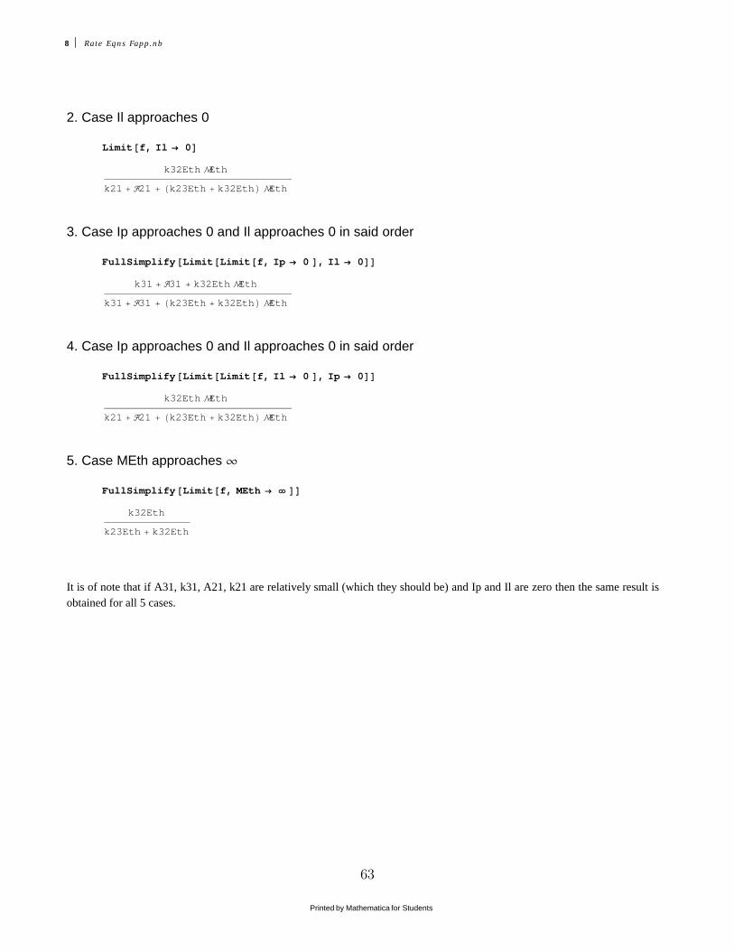
2. Case Il approaches 0
Limit@f, Il ® 0D
k32Eth MEth
k21 + A21 + Hk23Eth + k32EthL MEth
3. Case Ip approaches 0 and Il approaches 0 in said order
FullSimplify@Limit@Limit@f, Ip ® 0 D, Il ® 0DD
k31 + A31 + k32Eth MEth
k31 + A31 + Hk23Eth + k32EthL MEth
4. Case Ip approaches 0 and Il approaches 0 in said order
FullSimplify@Limit@Limit@f, Il ® 0 D, Ip ® 0DD
k32Eth MEth
k21 + A21 + Hk23Eth + k32EthL MEth
5. Case MEth approaches ¥
FullSimplify@Limit@f, MEth ® ¥ DD
k32Eth
k23Eth + k32Eth
It is of note that if A31, k31, A21, k21 are relatively small (which they should be) and Ip and Il are zero then the same result isobtained for all 5 cases.
8 Rate Eqns Fapp.nb
Printed by Mathematica for Students
63

Appendix B. Three Level DPAL Model Notebook for Rb
Sample Input and Without Sample Output
64
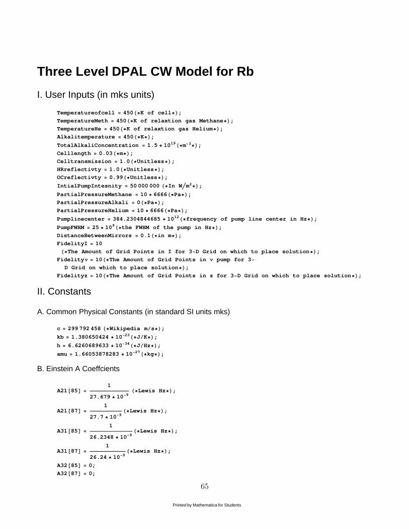
Three Level DPAL CW Model for Rb
I. User Inputs (in mks units)
Temperatureofcell = 450H*K of cell*L;TemperatureMeth = 450H*K of relaxtion gas Methane*L;TemperatureHe = 450H*K of relaxtion gas Helium*L;Alkalitemperature = 450H*K*L;TotalAlkaliConcentration = 1.5 * 1019H*m-3*L;Celllength = 0.03H*m*L;Celltransmission = 1.0H*Unitless*L;HRreflectivty = 1.0H*Unitless*L;OCreflectivty = 0.99H*Unitless*L;IntialPumpIntesnity = 50 000 000 H*In W�m2*L;PartialPressureMethane = 10 * 6666H*Pa*L;PartialPressureAlkali = 0H*Pa*L;PartialPressureHelium = 10 * 6666H*Pa*L;Pumplinecenter = 384.2304844685 * 1012H*frequency of pump line center in Hz*L;PumpFWHM = 25 * 109H*the FWHM of the pump in Hz*L;DistanceBetweenMirrors = 0.1H*in m*L;FidelityI = 10
H*The Amount of Grid Points in I for 3-D Grid on which to place solution*L;FidelityΝ = 10H*The Amount of Grid Points in Ν pump for 3-
D Grid on which to place solution*L;Fidelityz = 10H*The Amount of Grid Points in z for 3-D Grid on which to place solution*L;
II. Constants
A. Common Physical Constants (in standard SI units mks)
c = 299 792 458 H*Wikipedia m�s*L;kb = 1.380650424 * 10-23H*J�K*L;h = 6.6260689633 * 10-34H*J�Hz*L;amu = 1.66053878283 * 10-27H*kg*L;
B. Einstein A Coeffcients
A21@85D =1
27.679 * 10-9H*Lewis Hz*L;
A21@87D =1
27.7 * 10-9H*Lewis Hz*L;
A31@85D =1
26.2348 * 10-9H*Lewis Hz*L;
A31@87D =1
26.24 * 10-9H*Lewis Hz*L;
A32@85D = 0;
A32@87D = 0;
III. ParametersPrinted by Mathematica for Students
65

III. Parameters
A. Enviromental Paremeters
temp = 294.15H*K*L;tempcell = Temperatureofcell;
celloutsidepressure = 101.3 * 103 H*Pa*L;
B. Design Parameters
celllength = CelllengthH*m*L;celltransmission = CelltransmissionH*Unitless*L;hrreflectivty = HRreflectivtyH*Unitless*L;ocreflectivty = OCreflectivtyH*Unitless*L;Atomicmass@87D = 86.909180527 H*Lewis amu*L;Atomicmass@85D = 84.911789738H*Lewis amu*L;n = 1. H*index of refraction Unitless*L;ng = 1.H* group index of refraction Unitless*L;Ν21 = 377.1074635 * 1012 H*frequency 21 tranisition Lewis in Hz*L ;
Ν31 = 384.2304844685 * 1012H*Lewis Hz*L;Ν32 = 7.123020968 * 1012H*Lewis Hz*L;distance = DistanceBetweenMirrors ;
C. Laser and Cell Input Parameters
H*If you wish to add more species you must do so in II. C. , I. D., and in V. A.*LTotalAlkaliConcentration = TotalAlkaliConcentration H*In m-3*L;
tempMeth = TemperatureMethH*K*L;MMeth = PartialPressureMethane H*Partial Pressure of Methane in Pa*L;MMeth = 16.04246 * amuH*Mass of Methane Lewis kg*L;ΓMeth1 = 218 304.576H*For Rb87 and D1 manifold@iso?D in Hz�Pa Hager*L;ΓMeth2 = 196 549.137H*For Rb87 and D2 manifold@iso?Din Hz�Pa Hager*L;∆Me1 = -59 459.4595; H*Hz�Pa Collision induced shift D1 Hager*L∆Me2 = -52 552.5526; H*Hz�Pa Collision induced shift D2 Hager*L
tempAlk = AlkalitemperatureH*K*L;MAlk = PartialPressureAlkali; H*Partial Pressure of Alkali in Pa*LMAlk = 85.4678; H*Mass of Alkali function of iso? in kg*LΓAlk1 = 0H* in Hz�Pa*L;ΓAlk2 = 0H* in Hz�Pa*L;
tempHe = TemperatureHeH*K*L;MHe = PartialPressureHeliumH*Partial Pressure of Helium in Pa*L;MHe = 4.002602 * amuH*Mass of Helium in kg*L;ΓHe1 = 141 785.446H*For Rb87 and D1 manifold@iso?D in Hz�Pa Hager*L;ΓHe2 = 150 037.509H*For Rb87 and D2 manifold@iso?D in Hz�Pa Hager*L;∆He1 = 35 333.8335; H*Hz�Pa Collision induced shift D1 Hager*L∆He2 = 2775.69392; H*Hz�Pa Collision induced shift D2 Hager*L
D. Diode Input Lineshape
2 ThreelevelCWModelNDSOLVEgapproxEqnsLoopedShootingNDsolveWorkingLasingRigrodtexapp.nb
Printed by Mathematica for Students
66

D. Diode Input Lineshape
gIp0@Ν_D :=Π
2PumpFWHM 1 + ErfB
Pumplinecenter
2 PumpFWHM
F-1
ExpB-HΝ - PumplinecenterL2
2 PumpFWHM2F;
H*This is the Input Lineshape function for
gaussian distribution normalized to 1 and is unitless*LH*gIp0@Ν_D:=UnitStep@Ν-Ν31+PumpFWHM�2D*UnitStep@Ν31+PumpFWHM�2-ΝDH*This is a square wave and may be substituted*L*LIp0 = IntialPumpIntesnityH*W�m2*L;PlotAgIp0@ΝD, 8Ν, Ν31 - PumpFWHM * 3, Ν31 + PumpFWHM * 3<,PlotLabel ® "gpumpHΝL vs. Freq. ", AxesLabel ® 9gpAΝpE, Hz=E
IV. Kinetics
A. k Coeffcients (quenching rates only)
k21rate@1D = 0 � Hkb * tempMethLH* Methane Hz input the k rate in m3�s*L;k31rate@1D = 0 � Hkb * tempMethLH* Methane Hz input the k rate in m3�s*L;k21rate@2D = 0 � Hkb * tempHeLH* Helium Hz input the k rate in m3�s*L;k31rate@2D = 0 � Hkb * tempHeLH* Helium Hz input the k rate in m3�s*L;k21rate@3D = 0 � Hkb * tempAlkLH* Alkali Hz input the k rate in m3�s*L;k31rate@3D = 0 � Hkb * tempAlkLH* Alkali Hz input the k rate in m3�s*L;k21 := Sum@k21rate@speciesD * M@speciesD, 8species, 1, speciesmax, 1<D;k31 := Sum@k31rate@speciesD * M@speciesD, 8species, 1, speciesmax, 1<D;
B. Energy Differences D manifold states
DE21 = h * Ν21H*J*L;DE31 = h * Ν31H*J*L;DE32 = h * Ν32H*J*L;
C. Boltzmann Ratios
g3 = 4.H*Unitless*L;g2 = 2.H*Unitless*L;g1 = 2.H*Unitless*L;
f21 =g1
g2* ã
-DE21
kb*temp H*Unitless*L;
f31 =g1
g3* ã
-DE31
kb*temp H*Unitless*L;
f32 =g2
g3* ã
-DE32
kb*temp H*Unitless*L;
ThreelevelCWModelNDSOLVEgapproxEqnsLoopedShootingNDsolveWorkingLasingRigrodtexapp.nb 3
Printed by Mathematica for Students
67

D. k Coeffcients (for partner species on the 3 and 2 levels)
H*If you wish to add more species you must do so in II. C. , I. D., and ine V. A.*Lk32Meth@85D = 3.16 * 10-16 � Hkb * tempMethLH*Hager provided the number listed in m^3�s,but the value of the coeffcient is in Hz�Pa*L;
k32Meth@87D = 3.16 * 10-16 � Hkb * tempMethLH*Hager provided the number listed in m^3�s,but the value of the coeffcient is in Hz�Pa*L;
k23Meth@85D = k32Meth@85D * f32H*Hz�Pa*L;k23Meth@87D = k32Meth@87D * f32H*Hz�Pa*L;k32He@85D = 1.1776 * 106H*Hz�Pa*L;k32He@87D = 1.1776 * 106H*Hz�Pa*L;k23He@85D = k32He@85D * f32H*Hz�Pa*L;k23He@87D = k32He@87D * f32H*Hz�Pa*L;k32Alk@85D = 0H*Hz�Pa*L;k32Alk@87D = 0H*Hz�Pa*L;k23Alk@85D = k32Alk@85D * f32H*Hz�Pa*L;k23Alk@87D = k32Alk@87D * f32H*Hz�Pa*L;
V. Lineshape, Emission, and Absorbtion Cross Sections
A. Transition Lineshape
H*Einstein B coeffs based on the A coeff and the frequncy in Hz*L
B21@Ν_, iso_D :=c3 * A21@isoD
n2 * ng * 8 Π * h * Ν3H*m3�J*s2 or m�kg which are the same*L;
B12@Ν_, iso_D := g2 � g1 * B21@Ν, isoDH*m3�J*s2 or m�kg*L;
B31@Ν_, iso_D :=c3 * A31@isoD
n2 * ng * 8 Π * h * Ν3H*m3�J*s2 or m�kg*L;
B13@Ν_, iso_D := g3 � g1 * B31@Ν, isoDH*m3�J*s2 or m�kg*L;Τrad21@iso_D := HA21@isoDL-1H*s*L;Τrad31@iso_D := HA31@isoDL-1H*s*L;Τrad32 = ¥H*s*L;
H*Lorentzian Linewidth for transitions*L
DΝl21 @iso_D :=1
2 Π
1
Τrad21@isoD+ ΓMeth1 * MMeth *
tempMeth
temp
1�2+
ΓHe1 * MHe *tempHe
temp
1�2+ ΓAlk1 * MAlk *
tempAlk
temp
1�2H*Hz*L;
DΝl31 @iso_D :=1
2 Π
1
Τrad31@isoD+ ΓMeth2 * MMeth *
tempMeth
temp
1�2+
ΓHe2 * MHe *tempHe
temp
1�2+ ΓAlk2 * MAlk *
tempAlk
temp
1�2H*Hz*L;
Mass@85D = 84.911789738 * amuH*Lewis in kg*L;Mass@87D = 86.909180527 * amu H*Lewis in kg*L;
4 ThreelevelCWModelNDSOLVEgapproxEqnsLoopedShootingNDsolveWorkingLasingRigrodtexapp.nb
Printed by Mathematica for Students
68

H*Hyperfine corrections to frequency for 87 and 85 rb indexed
by F'' for low and F' for ups. Note:Fold is F'' or S1�2 level*LΝhyD2low@2, 87D = 2.563005979089114 * 109H*Hz*L;ΝhyD2low@1, 87D = -4.271676631815196 * 109H*Hz*L;ΝhyD2up@3, 87D = 193.740846 * 106H*Hz*L;ΝhyD2up@2, 87D = 72.911332 * 106H*Hz*L;ΝhyD2up@1, 87D = -229.851856 * 106H*Hz*L;ΝhyD2up@0, 87D = -302.073888 * 106H*Hz*L;ΝhyD1low@2, 87D = 2.563005979089114 * 109H*Hz*L;ΝhyD1low@1, 87D = -4.271676631815196 * 109H*Hz*L;ΝhyD1up@2, 87D = 306.246 * 106H*Hz*L;ΝhyD1up@1, 87D = -510.410 * 106H*Hz*L;
ΝhyD2low@3, 85D = 1.26488516325 * 109H*Hz*L;ΝhyD2low@2, 85D = -1.770843922835 * 109H*Hz*L;ΝhyD2up@4, 85D = 100.20544 * 106H*Hz*L;ΝhyD2up@3, 85D = 20.43551 * 106H*Hz*L;ΝhyD2up@2, 85D = -83.83534 * 106H*Hz*L;ΝhyD2up@1, 85D = -113.20884 * 106H*Hz*L;ΝhyD1low@3, 85D = 1.26488516325 * 109H*Hz*L;ΝhyD1low@2, 85D = -1.770843922835 * 109H*Hz*L;ΝhyD1up@3, 85D = 150.65971 * 106H*Hz*L;ΝhyD1up@2, 85D = -210.492399 * 106H*Hz*L;
ThreelevelCWModelNDSOLVEgapproxEqnsLoopedShootingNDsolveWorkingLasingRigrodtexapp.nb 5
Printed by Mathematica for Students
69

H*Line positions for hyperfine lines need several enteries 1,2,3,
4 for Fnews and Folds HThese are usually F' and F'' in literature where F is I ,
the nucler spin, + J, the angular momentum*LH*Νhy21@Fold ,Fnew ,D,isoD=:;*LH*Νhy31@Fold ,Fnew ,D,isoD=:;*LΝhy21@Fold_ , Fnew_ , D_ , iso_D := Ν21 - HΝhyD1low@Fold , isoDL + ΝhyD1up@Fnew , isoDH*Hz*L;Νhy31@Fold_ , Fnew_ , D_ , iso_D := Ν31 - HΝhyD2low@Fold , isoDL + ΝhyD2up@Fnew , isoDH*Hz*L;DΝd21 @Fold_ , Fnew_ , D_ , iso_D :=
Νhy21@Fold , Fnew , D, isoD *8 * kb * tempcell * Log@2D
Mass@isoD * c2
1
2
H*Hz*L;
DΝd31 @Fold_ , Fnew_ , D_ , iso_D := Νhy31@Fold , Fnew , D, isoD *8 * kb * tempcell * Log@2D
Mass@isoD * c2
1
2
H*Hz*L;
a21@Ν_, Fold_ , Fnew_ , D_ , iso_D := HLog@2DL1
2 *DΝl21 @isoD
DΝd21 @Fold , Fnew , D, isoDH*Unitless*L;
u21@Ν_, Fold_ , Fnew_ , D_ , iso_D := 2 * HLog@2DL1
2 *
KΝ - Νhy21@Fold , Fnew , D, isoDH*+∆Me1*MMeth*J tempMeth
tempN1�2
+∆He1*MHe*J tempHe
tempN1�2
*LO �DΝd21 @Fold , Fnew , D, isoDH*Unitless*L;
z21@Ν_, Fold_ , Fnew_ , D_ , iso_D := a21@Ν, Fold , Fnew , D, isoD + ä * u21@Ν, Fold , Fnew , D, isoDH*Unitless*L;
a31@Ν_, Fold_ , Fnew_ , D_ , iso_D := HLog@2DL1
2 *DΝl31 @isoD
DΝd31 @Fold , Fnew , D, isoDH*Unitless*L;
u31@Ν_, Fold_ , Fnew_ , D_ , iso_D := 2 * HLog@2DL1
2 *
KΝ - Νhy31@Fold , Fnew , D, isoDH*+∆Me2*MMeth*J tempMeth
tempN1�2
+∆He2*MHe*J tempHe
tempN1�2
*LO �DΝd31 @Fold , Fnew , D, isoDH*Unitless*L;
z31@Ν_, Fold_ , Fnew_ , D_ , iso_D := a31@Ν, Fold , Fnew , D, isoD + ä * u31@Ν, Fold , Fnew , D, isoDH*Unitless*L;
H*The lineshape of each transition. These functions represent
sets of functions for each transition indexed by there hyperfine
compenents F' and F'' and D the manifold or Fnew and Fold and D*L
g21@Ν_, Fold_ , Fnew_ , 1, iso_D := NIntegrateBMass@isoD
2 Π * kb * temp
1�2* 1012 *
DΝl21 @isoD � I2 Π * IHΝ - Νhy21@Fold , Fnew , 1, isoD - Νhy21@Fold , Fnew , 1, isoD * vz � cL2+
HDΝl21 @isoD � 2L2MM, 9vz, -106, 106=F � 1012H* in s*L;
g31@Ν_, Fold_ , Fnew_ , 2, iso_D := NIntegrateBMass@isoD
2 Π * kb * temp
1�2* 1012 *
DΝl31 @isoD � I2 Π * IHΝ - Νhy31@Fold , Fnew , 2, isoD - Νhy31@Fold , Fnew , 2, isoD * vz � cL2+
HDΝl31 @isoD � 2L2MM, 9vz, -1010, 1010=F � 1012H*in s*L;
6 ThreelevelCWModelNDSOLVEgapproxEqnsLoopedShootingNDsolveWorkingLasingRigrodtexapp.nb
Printed by Mathematica for Students
70

g21approx@Ν_, Fold_ , Fnew_ , 1, iso_D :=4 Log@2D
Π
1�2 1
DΝd21 @Fold , Fnew , 1, isoDReAã
Hz21@Ν,Fold ,Fnew ,1,isoDL2 Erfc@z21@Ν, Fold , Fnew , 1, isoDDEH*s*L;
g31approx@Ν_, Fold_ , Fnew_ , 2, iso_D :=4 Log@2D
Π
1�2 1
DΝd31 @Fold , Fnew , 2, isoDReAã
Hz31@Ν,Fold ,Fnew ,2,isoDL2 Erfc@z31@Ν, Fold , Fnew , 2, isoDDEH*s*L;
gapproxfix21@Ν_, Fold_ , Fnew_ , 1, iso_D :=
If@g21approx@Ν, Fold , Fnew , 1, isoD === Underflow@D,0, g21approx@Ν, Fold , Fnew , 1, isoDDH*s*L;
gapproxfix31@Ν_, Fold_ , Fnew_ , 2, iso_D := If@g31approx@Ν, Fold , Fnew , 2, isoD ===
Underflow@D, 0, g31approx@Ν, Fold , Fnew , 2, isoDDH*s*L;
H*PlotA8gapproxfix21@Ν,1,1,1,87D,gapproxfix21@Ν,1,2,1,87D,gapproxfix21@Ν,2,2,1,87D,gapproxfix21@Ν,2,1,1,87D<,9Ν,Νhy21@2,2,1,87D+2*109,Νhy21@1,1,1,87D-2*109=,
PlotRange®99Νhy21@1,2,1,87D-109,Νhy21@2,1,1,87D+109=,80,gapproxfix21@Νhy21@1,2,1,87D,2,2,1,87D*2<=E
PlotA8gapproxfix31@Ν,1,0,2,87D,gapproxfix31@Ν,1,1,2,87D,gapproxfix31@Ν,1,2,2,87D,gapproxfix31@Ν,2,2,2,87D,gapproxfix31@Ν,2,1,2,87D,gapproxfix31@Ν,2,3,2,87D<,
9Ν,Νhy31@2,2,2,87D-2*109,Νhy31@1,1,2,87D+2*109=,PlotRange®99Νhy31@2,2,2,87D+2*109,Νhy31@1,1,2,87D-2*109=,
80,gapproxfix31@Νhy31@2,2,2,87D,2,2,2,87D*2<=E*L
ThreelevelCWModelNDSOLVEgapproxEqnsLoopedShootingNDsolveWorkingLasingRigrodtexapp.nb 7
Printed by Mathematica for Students
71

B. Absorbtion Cross Section
i. Hyperfine Structure
H*S@Fold ,Fnew ,D,isoD is the relative line strength All are unitless*L
S@1, 1, 1, 87D =1
6H*Unitless*L;
S@1, 2, 1, 87D =5
6;
S@2, 2, 1, 87D =1
2;
S@2, 1, 1, 87D =1
2;
S@1, 0, 2, 87D =1
6;
S@1, 1, 2, 87D =5
12;
S@1, 2, 2, 87D =5
12;
S@1, 3, 2, 87D = 0;
S@2, 0, 2, 87D = 0;
S@2, 1, 2, 87D =1
20;
S@2, 2, 2, 87D =1
4;
S@2, 3, 2, 87D =7
10;
S@2, 2, 1, 85D =2
9;
S@2, 3, 1, 85D =7
9;
S@3, 2, 1, 85D =5
9;
S@3, 3, 1, 85D =4
9;
8 ThreelevelCWModelNDSOLVEgapproxEqnsLoopedShootingNDsolveWorkingLasingRigrodtexapp.nb
Printed by Mathematica for Students
72

S@2, 1, 2, 85D =3
10;
S@2, 2, 2, 85D =7
18;
S@2, 3, 2, 85D =14
45;
S@2, 4, 2, 85D = 0;
S@3, 1, 2, 85D = 0;
S@3, 2, 2, 85D =5
63;
S@3, 3, 2, 85D =5
18;
S@3, 4, 2, 85D =9
14;
H* *L
H*hyperfine line strengths for structure
need them for each forbidden transitions S = 0*LPlotA8gapproxfix21@Ν, 1, 1, 1, 87D * S@1, 1, 1, 87D + gapproxfix21@Ν, 1, 2, 1, 87D * S@1, 2, 1, 87D +
gapproxfix21@Ν, 2, 2, 1, 87D * S@2, 2, 1, 87D + gapproxfix21@Ν, 2, 1, 1, 87D * S@2, 1, 1, 87D<,8Ν, Νhy21@2, 2, 1, 87D + PumpFWHM, Νhy21@1, 1, 1, 87D - PumpFWHM<,PlotRange ® 88Νhy21@2, 2, 1, 87D + PumpFWHM, Νhy21@1, 1, 1, 87D - PumpFWHM<,
80, gapproxfix21@Νhy21@2, 2, 1, 87D, 2, 2, 1, 87D * 1<<,PlotLabel ® "g21HΝL vs. Freq. For 87Rb", AxesLabel ® 8Frequency @HzD, g@ΝD @unitlessD<E
PlotA8gapproxfix21@Ν, 2, 2, 1, 85D * S@2, 2, 1, 85D + gapproxfix21@Ν, 2, 3, 1, 85D * S@2, 3, 1, 85D +
gapproxfix21@Ν, 3, 3, 1, 85D * S@3, 3, 1, 85D + gapproxfix21@Ν, 3, 2, 1, 85D * S@3, 2, 1, 85D<,8Ν, Νhy21@3, 3, 1, 85D + PumpFWHM, Νhy21@2, 2, 1, 85D - PumpFWHM<,PlotRange ® 88Νhy21@3, 3, 1, 85D + PumpFWHM, Νhy21@2, 2, 1, 85D - PumpFWHM<,
80, gapproxfix21@Νhy21@2, 2, 1, 85D, 2, 2, 1, 85D * 1<<,PlotLabel ® "g21HΝL vs. Freq. For 85Rb", AxesLabel ® 8Frequency @HzD, g@ΝD @unitlessD<E
PlotA8gapproxfix31@Ν, 1, 0, 2, 87D * S@1, 0, 2, 87D + gapproxfix31@Ν, 1, 1, 2, 87D * S@1, 1, 2, 87D +
gapproxfix31@Ν, 1, 2, 2, 87D * S@1, 2, 2, 87D + gapproxfix31@Ν, 2, 2, 2, 87D * S@2, 2, 2, 87D +
+ <,
ThreelevelCWModelNDSOLVEgapproxEqnsLoopedShootingNDsolveWorkingLasingRigrodtexapp.nb 9
Printed by Mathematica for Students
73

gapproxfix31@Ν, 2, 1, 2, 87D * S@2, 1, 2, 87D + gapproxfix31@Ν, 2, 3, 2, 87D * S@2, 3, 2, 87D<,8Ν, Νhy31@2, 2, 2, 87D + PumpFWHM, Νhy31@1, 1, 2, 87D - PumpFWHM<,PlotRange ® 88Νhy31@2, 2, 2, 87D + PumpFWHM, Νhy31@1, 1, 2, 87D - PumpFWHM<,
80, gapproxfix31@Νhy31@2, 2, 2, 87D, 2, 2, 2, 87D * 1<<,PlotLabel ® "g31HΝL vs. Freq. For 87Rb", AxesLabel ® 8Frequency @HzD, g@ΝD @unitlessD<E
PlotA8gapproxfix31@Ν, 2, 1, 2, 85D * S@2, 1, 2, 85D + gapproxfix31@Ν, 2, 2, 2, 85D * S@2, 2, 2, 85D +
gapproxfix31@Ν, 2, 3, 2, 85D * S@2, 3, 2, 85D + gapproxfix31@Ν, 3, 3, 2, 85D * S@3, 3, 2, 85D +
gapproxfix31@Ν, 3, 2, 2, 85D * S@3, 2, 2, 85D + gapproxfix31@Ν, 3, 4, 2, 85D * S@3, 4, 2, 85D<,8Ν, Νhy31@3, 3, 2, 85D + PumpFWHM, Νhy31@2, 2, 2, 85D - PumpFWHM<,PlotRange ® 88Νhy31@3, 3, 2, 85D + PumpFWHM, Νhy31@2, 2, 2, 85D - PumpFWHM<,
80, gapproxfix31@Ν31, 3, 3, 2, 85D * 15<<,PlotLabel ® "g31HΝL vs. Freq. For 85Rb", AxesLabel ® 8Frequency @HzD, g@ΝD @unitlessD<E
10 ThreelevelCWModelNDSOLVEgapproxEqnsLoopedShootingNDsolveWorkingLasingRigrodtexapp.nb
Printed by Mathematica for Students
74

ii. Statistical isotope distribution
fiso@85D = 0.7217H*Unitless*L;fiso@87D = 0.2783H*Unitless*L;
Fnewmin @1, 87D = 1H*Unitless*L;Fnewmax @1, 87D = 2H*Unitless*L;Foldmin @1, 87D = 1H*Unitless*L;Foldmax @1, 87D = 2H*Unitless*L;
Fnewmin @2, 87D = 0H*Unitless*L;Fnewmax @2, 87D = 3H*Unitless*L;Foldmin @2, 87D = 1H*Unitless*L;Foldmax @2, 87D = 2H*Unitless*L;
Fnewmin @1, 85D = 2H*Unitless*L;Fnewmax @1, 85D = 3H*Unitless*L;Foldmin @1, 85D = 2H*Unitless*L;Foldmax @1, 85D = 3H*Unitless*L;
Fnewmin @2, 85D = 1H*Unitless*L;Fnewmax @2, 85D = 4H*Unitless*L;Foldmin @2, 85D = 2H*Unitless*L;Foldmax @2, 85D = 3H*Unitless*L;
isomin = 85H*Unitless*L;isomax = 87H*Unitless*L;isostep = 2H*Unitless*L;
EngD2@Fold_ , iso_D := h * HΝ31 - ΝhyD2low@Fold , isoD LH*The energy of a given F'' state in J*L;
EngD1@Fold_ , iso_D := h * HΝ21 - ΝhyD1low@Fold , isoDLH*J*L;
ftotD1@85D = âFold =Foldmin @1,85D
Foldmax @1,85DH2 Fold + 1L * ã
-EngD1@Fold ,85Dkb*temp H*Unitless*L;
ftotD1@87D = âFold =Foldmin @1,87D
Foldmax @1,87DH2 Fold + 1L * ã
-EngD1@Fold ,87Dkb*temp H*Unitless*L;
ftotD2@85D := âFold =Foldmin @2,85D
Foldmax @2,85DH2 Fold + 1L * ã
-EngD2@Fold ,85Dkb*temp H*Unitless*L;
ftotD2@87D := âFold =Foldmin @2,87D
Foldmax @2,87DH2 Fold + 1L * ã
-EngD2@Fold ,87Dkb*temp H*Unitless*L;
ff21@Fold_ , iso_D :=H2 Fold + 1L * ã
-EngD1@Fold ,isoDkb*temp
ftotD1@isoDH*stat dis among F states will need several enteries for eachH*Unitless*L*L
ff31@Fold_ , iso_D :=H2 Fold + 1L * ã
-EngD2@Fold ,isoDkb*temp
ftotD2@isoDH*stat dis among F states will need several enteries for eachH*Unitless*L*L
iii. Cross Sections (in m2M
ThreelevelCWModelNDSOLVEgapproxEqnsLoopedShootingNDsolveWorkingLasingRigrodtexapp.nb 11
Printed by Mathematica for Students
75
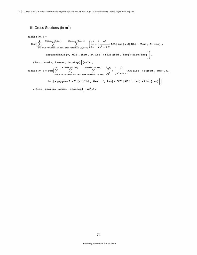
iii. Cross Sections (in m2M
Σ12abs@Ν_D =
SumBâD=1
1
âFold =Foldmin @D,isoD
Foldmax @D,isoDâ
Fnew =Fnewmin @D,isoD
Fnewmax @D,isoD g2
g1*
c2
Ν2 * 8 Π
A21@isoD * S@Fold , Fnew , D, isoD *
gapproxfix21@Ν, Fold , Fnew , D, isoD * ff21@Fold , isoD * fiso@isoD ,
8iso, isomin, isomax, isostep<FH*m2*L;
Σ13abs@Ν_D = SumBâD=2
2
âFold =Foldmin @D,isoD
Foldmax @D,isoDâ
Fnew =Fnewmin @D,isoD
Fnewmax @D,isoD g3
g1*
c2
Ν2 * 8 Π
A31@isoD * S@Fold , Fnew , D,
isoD * gapproxfix31@Ν, Fold , Fnew , D, isoD * ff31@Fold , isoD * fiso@isoD
, 8iso, isomin, isomax, isostep<FH*m2*L;
12 ThreelevelCWModelNDSOLVEgapproxEqnsLoopedShootingNDsolveWorkingLasingRigrodtexapp.nb
Printed by Mathematica for Students
76

C. Emission Cross Sections
Σ21ems@Ν_D =g1
g2Σ12abs@ΝDH*m2*L;
Σ31ems@Ν_D =g1
g3Σ13abs@ΝDH*m2*L;
H*DoAPrintAΣ21emsAΝhy21@2,2,1,87D-106+i*105EE,8i,100<E;*LH*trapend=2*1011;
trapstep=109;
trapstart=Νhy21@2,2,1,87D-109;trapend
trapend�trapstep*SumAΣ21emsAΝhy21@2,2,1,87D-1011+lE,8l,0,trapend,trapstep<E*L
H*PlotA8Σ21ems@Ν_D<,9Ν,Νhy21@2,2,1,87D-109,Νhy21@2,2,1,87D+109=,PlotRange®99Νhy21@2,2,1,87D-109,Νhy21@2,2,1,87D+109=,90,2*10-7==E*L
H*NIntegrate@Σ21ems@Ν_D,8Ν,Νhy21@2,2,1,87D,Νhy21@1,1,1,87D<,Method®"TrapezoidalRule"D*Lgapproxfixtotal21@Ν_D =
SumBâD=1
1
âFold =Foldmin @D,isoD
Foldmax @D,isoDâ
Fnew =Fnewmin @D,isoD
Fnewmax @D,isoDgapproxfix21@Ν, Fold , Fnew , D, isoD *
S@Fold , Fnew , D, isoD * fiso@isoD * ff21@Fold , isoD, 8iso, isomin, isomax, isostep<F;
gapproxfixtotal31@Ν_D = SumBâD=2
2
âFold =Foldmin @D,isoD
Foldmax @D,isoDâ
Fnew =Fnewmin @D,isoD
Fnewmax @D,isoDgapproxfix31@
Ν, Fold , Fnew , D, isoD * S@Fold , Fnew , D, isoD *
fiso@isoD ff31@Fold , isoD, 8iso, isomin, isomax, isostep<F;
PlotA8gapproxfixtotal31@Ν31 + ΝD, gIp0@Ν31 + ΝD<, 8Ν, -2 * PumpFWHM, 2 * PumpFWHM<,PlotRange ® 88-PumpFWHM * 2, PumpFWHM * 2<, 80, gapproxfixtotal31@Νhy31@2, 2, 2, 87DD * 3<<,PlotLabel ® StyleA"g31HΝLHBlueL and gpumpHΝpLHRedL for Rb vs. Freq.", 24E,LabelStyle ® Directive@LargeD, AxesLabel ® 8Frequency @HzD, g@ΝD @unitlessD<,LabelStyle ® Directive@LargeD, AxesOrigin ® 8-PumpFWHM * 2, 0<E
PlotAΣ31ems@Ν31 + ΝD, 8Ν, -2 * PumpFWHM, 2 * PumpFWHM<,PlotRange ® 88-2 * PumpFWHM, 2 * PumpFWHM<, 80, Σ31ems@Νhy31@2, 2, 2, 87DD * 3<<,PlotLabel ® Style@"Σ31ems@ΝD vs. Freq.", 24D, LabelStyle ® Directive@LargeD,AxesLabel ® 9 Frequency@ HzD , Σ31ems@ΝD Am2E=, LabelStyle ® Directive@LargeD,AxesOrigin ® 8-2 * PumpFWHM, 0<, PlotPoints ® 400E
Plot@gapproxfixtotal21@Ν21 + ΝD, 8Ν, -1 � 5 * PumpFWHM, 1 � 4 * PumpFWHM<,PlotLabel ® Style@"g21HΝL For Rb vs. Freq.", 24D,AxesLabel ® 8Frequency @HzD, g@ΝD @unitlessD<, LabelStyle ® Directive@LargeD,AxesOrigin ® 8-PumpFWHM * 1 � 5, 0<, PlotRange ®
88-PumpFWHM * 1 � 5, PumpFWHM * 1 � 4<, 80, gapproxfixtotal21@Νhy21@1, 1, 1, 87DD * 10<<DPlotAΣ21ems@Ν21 + ΝD, 8Ν, -2 * PumpFWHM, +2 * PumpFWHM<,PlotRange ® 88-PumpFWHM * 2, PumpFWHM * 2<, 80, Σ21ems@Νhy21@1, 1, 1, 87DD * 6<<,PlotLabel ® Style@"Σ21emsHΝL vs. Freq.", 24D, AxesLabel ® 9 Frequency@ HzD , Σ21ems@ΝDAm2E=,LabelStyle ® Directive@LargeD, AxesOrigin ® 8-PumpFWHM * 2, 0<, PlotPoints ® 400E
ThreelevelCWModelNDSOLVEgapproxEqnsLoopedShootingNDsolveWorkingLasingRigrodtexapp.nb 13
Printed by Mathematica for Students
77

D. Cavity-Mode Spacing
DΝfsr =c
2 * n * distance;
Νmaxgain = Ν �. LastAFindMaximumAΣ21ems@ΝD, 9Ν, Ν21 - 1010, Ν21 + 1010=EE;qmaxgain = Round@Νmaxgain � DΝfsr D;Νlaser = qmaxgain * DΝfsr ;
PlotBΝlaser
Pumplinecenter
Σ21ems@Ν21 + ΝDΣ31ems@Pumplinecenter + ΝD
, 8Ν, -2 * PumpFWHM, 2 * PumpFWHM<,
PlotLabel ® Style@"Η The effciency factor vs. Frequency in Hz", 24D,AxesLabel ® 8Freq@HzD, Η<, LabelStyle ® Directive@LargeDF
14 ThreelevelCWModelNDSOLVEgapproxEqnsLoopedShootingNDsolveWorkingLasingRigrodtexapp.nb
Printed by Mathematica for Students
78

VII. Rate Equations Analysis, ODE Solutions, and System Outputs
H* *�
L
ThreelevelCWModelNDSOLVEgapproxEqnsLoopedShootingNDsolveWorkingLasingRigrodtexapp.nb 15
Printed by Mathematica for Students
79
A. Species Setups
H*If you wish to add more species you must do so in II. C. ,
I. D., and in V. A. Also rember the species numer H1,2,3...Lmust be the same for all coeffs and pressures. @2D must always
correspond to Heane for the species, but other sums do exist*Lk23@1, iso_D := k23Meth@isoDH*Hz*L;k23@2, iso_D := k23He@isoDH*Hz*L;k23@3, iso_D := k23Alk@isoDH*Hz*L;k32@1, iso_D := k32Meth@isoDH*Hz*L;k32@2, iso_D := k32He@isoDH*Hz*L;k32@3, iso_D := k32Alk@isoDH*Hz*L;M@1D = MMeth; H*Partial Pressures in Pa*LM@2D = MHeH*Pa*L;M@3D = MAlkH*Pa*L;speciesmax = 3H*Unitless*L;
16 ThreelevelCWModelNDSOLVEgapproxEqnsLoopedShootingNDsolveWorkingLasingRigrodtexapp.nb
Printed by Mathematica for Students
80

B. Rate Equations and Populations
Nt = TotalAlkaliConcentration H*in m-3*L;Il@z_D := Iplu@zD + Iminu@zDH*W�m2*L;H*Reqn1@N1_ ,N2_ ,N3_ D:=Ù
-¥
¥ Úspecies=1speciesmax
N3 *A31+N2 *A21 +
N3 *k31+N2 *k21+J-B13@ΝD*N1 *Ip+B31@ΝD*N3 *Ip+B21@ΝD*Il*JN2 -g2
g1N1 NNâΝ;
Reqn2@N1_ ,N2_ ,N3_ D:=Ù-¥
¥ Úspecies=1speciesmax
N3 *k32Meth*MMeth-N2 *k23Meth*MMeth-
N2 *A21-N2 *k21 -B21@ΝD*Il*JN2 -g2
g1N1 NâΝ;
Reqn3@N1_ ,N2_ ,N3_ D:=Ù-¥
¥ Úspecies=1speciesmax
-N3 *k32Meth*MMeth+N2 *k23Meth*MMeth-
N3 *A31-N3 *k31 +B13@ΝD*Ip*N1 -B31@ΝD*N3 *Ip âΝ;
Reqn4@N1_ ,N2_ ,N3_ D:=N1 +N2 +N3 ;
Solve@8Reqn2@N1 ,N2 ,N3 D,Reqn3@N1 ,N2 ,N3 D,Reqn4@N1 ,N2 ,N3 D<�80,0,Nt <,8N1 ,N2 ,N3 <D;f=
N2
N2 +N3;*L
Pop3@z_, Ν_, Νpump_ D = SumBSumBfiso@isoD *1
speciesmax*
- Nt -k21 - A21@isoD - k23@species, isoD M@speciesD -Il@zD Σ21ems@ΝlaserD
h Νlaser-
g2 Il@zD Σ21ems@ΝlaserDg1 h Νlaser
-g2 Il@zD Σ21ems@ΝlaserD
g1 h Νlaser-g3 Ip@zD Σ31ems@ΝpumpD
g1 h Νpump-
1
g1 h Νlaserg2 Nt Il@zD Σ21ems@ΝlaserD k21 + A21@isoD +
Il@zD Σ21ems@ΝlaserDh Νlaser
+
g2 Il@zD Σ21ems@ΝlaserDg1 h Νlaser
+g3 Ip@zD Σ31ems@ΝpumpD
g1 h Νpump�
- k32@species, isoD M@speciesD -g2 Il@zD Σ21ems@ΝlaserD
g1 h Νlaserk21 + A21@isoD +
Il@zD Σ21ems@ΝlaserDh Νlaser
+g2 Il@zD Σ21ems@ΝlaserD
g1 h Νlaser+g3 Ip@zD Σ31ems@ΝpumpD
g1 h Νpump+
-k21 - A21@isoD - k23@species, isoD M@speciesD -Il@zD Σ21ems@ΝlaserD
h Νlaser-
g2 Il@zD Σ21ems@ΝlaserDg1 h Νlaser
k31 + A31@isoD +g2 Il@zD Σ21ems@ΝlaserD
g1 h Νlaser+
+ ,
ThreelevelCWModelNDSOLVEgapproxEqnsLoopedShootingNDsolveWorkingLasingRigrodtexapp.nb 17
Printed by Mathematica for Students
81

Ip@zD Σ31ems@ΝpumpDh Νpump
+g3 Ip@zD Σ31ems@ΝpumpD
g1 h Νpump,
8species, 1, speciesmax, 1<F, 8iso, isomin, isomax, isostep<FH*m-3*L;
Pop2@z_, Ν_, Νpump_ D = SumBSumBfiso@isoD *1
speciesmax*
-Hg2 Nt Il@zD Σ21ems@ΝlaserDL � g1 h Νlaser -k21 - A21@isoD -
k23@species, isoD M@speciesD -Il@zD Σ21ems@ΝlaserD
h Νlaser-g2 Il@zD Σ21ems@ΝlaserD
g1 h Νlaser+
k32@species, isoD M@speciesD -g2 Il@zD Σ21ems@ΝlaserD
g1 h Νlaser
Nt -k21 - A21@isoD - k23@species, isoD M@speciesD -Il@zD Σ21ems@ΝlaserD
h Νlaser-
g2 Il@zD Σ21ems@ΝlaserDg1 h Νlaser
-g2 Il@zD Σ21ems@ΝlaserD
g1 h Νlaser-g3 Ip@zD Σ31ems@ΝpumpD
g1 h Νpump-
1
g1 h Νlaserg2 Nt Il@zD Σ21ems@ΝlaserD k21 + A21@isoD +
Il@zD Σ21ems@ΝlaserDh Νlaser
+
g2 Il@zD Σ21ems@ΝlaserDg1 h Νlaser
+g3 Ip@zD Σ31ems@ΝpumpD
g1 h Νpump�
-k21 - A21@isoD - k23@species, isoD M@speciesD -Il@zD Σ21ems@ΝlaserD
h Νlaser-
g2 Il@zD Σ21ems@ΝlaserDg1 h Νlaser
- k32@species, isoD M@speciesD -g2 Il@zD Σ21ems@ΝlaserD
g1 h Νlaserk21 + A21@isoD +
Il@zD Σ21ems@ΝlaserDh Νlaser
+g2 Il@zD Σ21ems@ΝlaserD
g1 h Νlaser+g3 Ip@zD Σ31ems@ΝpumpD
g1 h Νpump+
-k21 - A21@isoD - k23@species, isoD M@speciesD -Il@zD Σ21ems@ΝlaserD
h Νlaser-
g2 Il@zD Σ21ems@ΝlaserDg1 h Νlaser
k31 + A31@isoD +g2 Il@zD Σ21ems@ΝlaserD
g1 h Νlaser+
Ip@zD Σ31ems@ΝpumpDh Νpump
+g3 Ip@zD Σ31ems@ΝpumpD
g1 h Νpump,
8species, 1, speciesmax, 1<F, 8iso, isomin, isomax,
isostep<F ;
18 ThreelevelCWModelNDSOLVEgapproxEqnsLoopedShootingNDsolveWorkingLasingRigrodtexapp.nb
Printed by Mathematica for Students
82

isostep<FH*m-3*L;
Pop1@z_, Ν_, Νpump_ D = SumBSumBfiso@isoD *1
speciesmax*
Nt + Hg2 Nt Il@zD Σ21ems@ΝlaserDL � g1 h Νlaser -k21 - A21@isoD -
k23@species, isoD M@speciesD -Il@zD Σ21ems@ΝlaserD
h Νlaser-g2 Il@zD Σ21ems@ΝlaserD
g1 h Νlaser+
Nt -k21 - A21@isoD - k23@species, isoD M@speciesD -Il@zD Σ21ems@ΝlaserD
h Νlaser-
g2 Il@zD Σ21ems@ΝlaserDg1 h Νlaser
-g2 Il@zD Σ21ems@ΝlaserD
g1 h Νlaser-g3 Ip@zD Σ31ems@ΝpumpD
g1 h Νpump-
1
g1 h Νlaserg2 Nt Il@zD Σ21ems@ΝlaserD k21 + A21@isoD +
Il@zD Σ21ems@ΝlaserDh Νlaser
+
g2 Il@zD Σ21ems@ΝlaserDg1 h Νlaser
+g3 Ip@zD Σ31ems@ΝpumpD
g1 h Νpump�
- k32@species, isoD M@speciesD -g2 Il@zD Σ21ems@ΝlaserD
g1 h Νlaserk21 + A21@isoD +
Il@zD Σ21ems@ΝlaserDh Νlaser
+g2 Il@zD Σ21ems@ΝlaserD
g1 h Νlaser+g3 Ip@zD Σ31ems@ΝpumpD
g1 h Νpump+
-k21 - A21@isoD - k23@species, isoD M@speciesD -Il@zD Σ21ems@ΝlaserD
h Νlaser-
g2 Il@zD Σ21ems@ΝlaserDg1 h Νlaser
k31 + A31@isoD +g2 Il@zD Σ21ems@ΝlaserD
g1 h Νlaser+
Ip@zD Σ31ems@ΝpumpDh Νpump
+g3 Ip@zD Σ31ems@ΝpumpD
g1 h Νpump-
k32@species, isoD M@speciesD -g2 Il@zD Σ21ems@ΝlaserD
g1 h Νlaser
Nt -k21 - A21@isoD - k23@species, isoD M@speciesD -Il@zD Σ21ems@ΝlaserD
h Νlaser-
g2 Il@zD Σ21ems@ΝlaserDg1 h Νlaser
-g2 Il@zD Σ21ems@ΝlaserD
g1 h Νlaser-g3 Ip@zD Σ31ems@ΝpumpD
g1 h Νpump-
1
g1 h Νlaserg2 Nt Il@zD Σ21ems@ΝlaserD k21 + A21@isoD +
Il@zD Σ21ems@ΝlaserDh Νlaser
+
+ �
ThreelevelCWModelNDSOLVEgapproxEqnsLoopedShootingNDsolveWorkingLasingRigrodtexapp.nb 19
Printed by Mathematica for Students
83
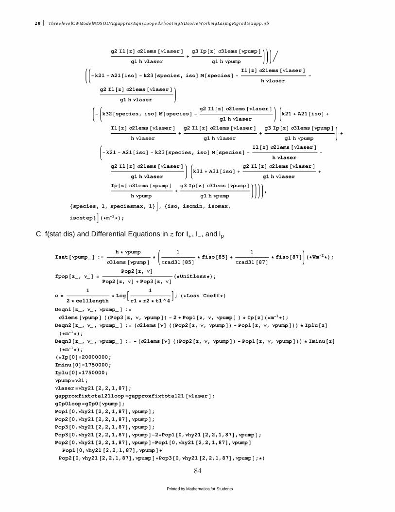
g2 Il@zD Σ21ems@ΝlaserDg1 h Νlaser
+g3 Ip@zD Σ31ems@ΝpumpD
g1 h Νpump�
-k21 - A21@isoD - k23@species, isoD M@speciesD -Il@zD Σ21ems@ΝlaserD
h Νlaser-
g2 Il@zD Σ21ems@ΝlaserDg1 h Νlaser
- k32@species, isoD M@speciesD -g2 Il@zD Σ21ems@ΝlaserD
g1 h Νlaserk21 + A21@isoD +
Il@zD Σ21ems@ΝlaserDh Νlaser
+g2 Il@zD Σ21ems@ΝlaserD
g1 h Νlaser+g3 Ip@zD Σ31ems@ΝpumpD
g1 h Νpump+
-k21 - A21@isoD - k23@species, isoD M@speciesD -Il@zD Σ21ems@ΝlaserD
h Νlaser-
g2 Il@zD Σ21ems@ΝlaserDg1 h Νlaser
k31 + A31@isoD +g2 Il@zD Σ21ems@ΝlaserD
g1 h Νlaser+
Ip@zD Σ31ems@ΝpumpDh Νpump
+g3 Ip@zD Σ31ems@ΝpumpD
g1 h Νpump,
8species, 1, speciesmax, 1<F, 8iso, isomin, isomax,
isostep<FH*m-3*L;
C. f(stat dis) and Differential Equations in z for I+, I-, and Ip
Isat@Νpump_ D :=h * Νpump
Σ31ems@ΝpumpD*
1
Τrad31@85D* fiso@85D +
1
Τrad31@87D* fiso@87D H*Wm-2*L;
fpop@z_, Ν_D =Pop2@z, ΝD
Pop2@z, ΝD + Pop3@z, ΝDH*Unitless*L;
Α =1
2 * celllength* LogB
1
r1 * r2 * t1^4F; H*Loss Coeff*L
Deqn1@z_, Ν_, Νpump_ D :=
Σ31ems@ΝpumpD HHPop3@z, Ν, ΝpumpDL - 2 * Pop1@z, Ν, ΝpumpD L * Ip@zDH*m-1*L;Deqn2@z_, Ν_, Νpump_ D := HΣ21ems@ΝD HHPop2@z, Ν, ΝpumpDL - Pop1@z, Ν, ΝpumpDLL * Iplu@zD
H*m-1*L;Deqn3@z_, Ν_, Νpump_ D := -HΣ21ems@ΝD HHPop2@z, Ν, ΝpumpDL - Pop1@z, Ν, ΝpumpDLL * Iminu@zD
H*m-1*L;H*Ip@0D=20000000;
Iminu@0D=1750000;
Iplu@0D=1750000;
Νpump=Ν31;
Νlaser=Νhy21@2,2,1,87D;gapproxfixtotal21loop=gapproxfixtotal21@ΝlaserD;gIp0loop=gIp0@ΝpumpD;Pop1@0,Νhy21@2,2,1,87D,ΝpumpD;Pop2@0,Νhy21@2,2,1,87D,ΝpumpD;Pop3@0,Νhy21@2,2,1,87D,ΝpumpD;Pop3@0,Νhy21@2,2,1,87D,ΝpumpD-2*Pop1@0,Νhy21@2,2,1,87D,ΝpumpD;Pop2@0,Νhy21@2,2,1,87D,ΝpumpD-Pop1@0,Νhy21@2,2,1,87D,ΝpumpD
Pop1@0,Νhy21@2,2,1,87D,ΝpumpD+
Pop2@0,Νhy21@2,2,1,87D,ΝpumpD+Pop3@0,Νhy21@2,2,1,87D,ΝpumpD;*L
D. NDSolve Routine for I+, I-, and Ip
20 ThreelevelCWModelNDSOLVEgapproxEqnsLoopedShootingNDsolveWorkingLasingRigrodtexapp.nb
Printed by Mathematica for Students
84

D. NDSolve Routine for I+, I-, and Ip
H*Ip@znotD�Ip0*gIp0@Ν31D,Iplu@znotD�Iminu@znotD,refl*Iplu@zfinalD�Iminu@zfinalD,Iplu@zD*Iminu@zD==Constant*Lt1 = celltransmissionH*Unitless*L;r1 = hrreflectivtyH*Unitless*L;r2 = ocreflectivtyH*Unitless*L;znot = 0.0H*m*L;zfinal = znot + celllengthH*m*L;
Νrange = 3 * PumpFWHM;
Νsteps = FidelityΝ;
Iplusteps = FidelityI;
Iplustepsize@Νpump_ D =Ip0 * gIp0@ΝpumpD � gIp0@PumplinecenterD
Iplusteps;
H*Ip0*gIp0@ΝpumpD�gIp0@Ν31DΝlaser=Νhy21@2,2,1,87D;
Νpump=Ν31;
Σ21emsloop=Σ21ems@ΝlaserD;Σ31emsloop=Σ31ems@ΝpumpD;gapproxfixtotal21loop=gapproxfixtotal21@ΝlaserD;gIp0loop=gIp0@ΝpumpD;
Intenfunc=NDSolveA9Deqn1@z,Νlaser,ΝpumpD�Ip'@zD,Deqn2@z,Νlaser,ΝpumpD�Iplu'@zD,Deqn3@z,Νlaser,ΝpumpD�Iminu'@zD,Ip@znotD�Ip0*gIp0@ΝpumpD�gIp0@Ν31D,Iplu@znotD�1000,
Iplu@znotD==r1*t12*Iminu@znotD=,8Ip@zD,Iplu@zD,Iminu@zD<,8z,znot,zfinal<E*L
ThreelevelCWModelNDSOLVEgapproxEqnsLoopedShootingNDsolveWorkingLasingRigrodtexapp.nb 21
Printed by Mathematica for Students
85
Percentdone = 0;
Νpumpcount = 1;
DoB:Iplucount = 1;
Σ21emsloop = Σ21ems@ΝlaserD;Σ31emsloop = Σ31ems@ΝpumpD;gapproxfixtotal21loop = gapproxfixtotal21@ΝlaserD;gIp0loop = gIp0@ΝpumpD;Νarray@ΝpumpcountD = Νpump;
DoB:
Intenfunc = NDSolveA9Deqn1@z, Νlaser, ΝpumpD � Ip'@zD,Deqn2@z, Νlaser, ΝpumpD � Iplu'@zD, Deqn3@z, Νlaser, ΝpumpD � Iminu'@zD, Ip@znotD �
Ip0 * gIp0@ΝpumpD � gIp0@PumplinecenterD, Iplu@znotD + Iminu@znotD � Ipluindex,
Iplu@znotD == r1 * t12 * Iminu@znotD=, 8Ip, Iplu, Iminu<, 8z, znot, zfinal<E;SaveIntenfunc@Νpumpcount, IplucountD = Intenfunc,
Iplucount = Iplucount + 1;
H* Percentdone2=Percentdone+100.
Νsteps*J Iplucount-1
IplustepsN,
Print@Percentdone2,"% Completed"D*L>
, 8Ipluindex, 0, Ip0 * gIp0@ΝpumpD � gIp0@PumplinecenterD, Iplustepsize@ΝpumpD<F,
Percentdone = 100 *Νpumpcount - 1.
Νsteps,
Print@Percentdone, "% Completed"D ,
Νpumpcount = Νpumpcount + 1>, :Νpump, Pumplinecenter - Νrange, Pumplinecenter + Νrange,
HPumplinecenter + ΝrangeL - HPumplinecenter - ΝrangeLΝsteps
>
F
0.% Completed
10.% Completed
20.% Completed
30.% Completed
40.% Completed
50.% Completed
60.% Completed
70.% Completed
80.% Completed
22 ThreelevelCWModelNDSOLVEgapproxEqnsLoopedShootingNDsolveWorkingLasingRigrodtexapp.nb
Printed by Mathematica for Students
86

E. Routine for Selecting the Best Solution from NDSolve
ClearAll@CurrentRoot, RootfindeqnDPercentdone = 0;
DoB:Rootfindeqn@Νpumpcount2 D = Ip0,
Do@8H*Print@ Evaluate@Iplu@zfinalD�.SaveIntenfunc@Νpumpcount2 ,Iplucount2DD===80.<D,*L
zarraytest@Νpumpcount2 , Iplucount2D = znot,
Iparraytest@Νpumpcount2 , Iplucount2D =
Evaluate@Ip@zarraytest@Νpumpcount2 , Iplucount2DD �.SaveIntenfunc@Νpumpcount2 , Iplucount2DD@@1DD,Ipnolasingarraytest@Νpumpcount2 , Iplucount2D = Evaluate@
Ip@zarraytest@Νpumpcount2 , Iplucount2DD �. SaveIntenfunc@Νpumpcount2 , 1DD@@1DD,Ipluarraytest@Νpumpcount2 , Iplucount2D =
Evaluate@Iplu@zarraytest@Νpumpcount2 , Iplucount2DD �.SaveIntenfunc@Νpumpcount2 , Iplucount2DD@@1DD,Iminuarraytest@Νpumpcount2 , Iplucount2D =
Evaluate@Iminu@zarraytest@Νpumpcount2 , Iplucount2DD �.SaveIntenfunc@Νpumpcount2 , Iplucount2DD@@1DD,
N1arraytest @Νpumpcount2 , Iplucount2D =
Pop1@zarraytest@Νpumpcount2 , Iplucount2D, Νlaser, Νarray@Νpumpcount2 DD �.8Ip@zarraytest@Νpumpcount2 , Iplucount2DD ® Iparraytest@Νpumpcount2 , Iplucount2D,Iplu@zarraytest@Νpumpcount2 , Iplucount2DD ® Ipluarraytest@Νpumpcount2 , Iplucount2D,Iminu@zarraytest@Νpumpcount2 , Iplucount2DD ®
Iminuarraytest@Νpumpcount2 , Iplucount2D<,N2arraytest @Νpumpcount2 , Iplucount2D =
Pop2@zarraytest@Νpumpcount2 , Iplucount2D, Νlaser, Νarray@Νpumpcount2 DD �.8Ip@zarraytest@Νpumpcount2 , Iplucount2DD ® Iparraytest@Νpumpcount2 , Iplucount2D,Iplu@zarraytest@Νpumpcount2 , Iplucount2DD ® Ipluarraytest@Νpumpcount2 , Iplucount2D,Iminu@zarraytest@Νpumpcount2 , Iplucount2DD ®
Iminuarraytest@Νpumpcount2 , Iplucount2D<,N3arraytest @Νpumpcount2 , Iplucount2D =
Pop3@zarraytest@Νpumpcount2 , Iplucount2D, Νlaser, Νarray@Νpumpcount2 DD �.8Ip@zarraytest@Νpumpcount2 , Iplucount2DD ® Iparraytest@Νpumpcount2 , Iplucount2D,Iplu@zarraytest@Νpumpcount2 , Iplucount2DD ® Ipluarraytest@Νpumpcount2 , Iplucount2D,Iminu@zarraytest@Νpumpcount2 , Iplucount2DD ®
Iminuarraytest@Νpumpcount2 , Iplucount2D<,Γtest@Νpumpcount2 , zarraytest@Νpumpcount2 , Iplucount2DD = Σ21ems@ΝlaserD *
HN2arraytest @Νpumpcount2 , Iplucount2D - N1arraytest @Νpumpcount2 , Iplucount2DL,If@
ThreelevelCWModelNDSOLVEgapproxEqnsLoopedShootingNDsolveWorkingLasingRigrodtexapp.nb 23
Printed by Mathematica for Students
87

Evaluate@Iplu@zfinalD �. SaveIntenfunc@Νpumpcount2 , Iplucount2DD@@1DD >= 0.,
CurrentRoot@Νpumpcount2 , Iplucount2D =
Hr2 * t1^2 * Evaluate@Iplu@zfinalD �. SaveIntenfunc@Νpumpcount2 , Iplucount2DD@@1DDL �HHEvaluate@Iminu@zfinalD �. SaveIntenfunc@Νpumpcount2 , Iplucount2DD@@1DDL +
0.00001L - 1
D,If@
Γtest@Νpumpcount2 , zarraytest@Νpumpcount2 , Iplucount2DD - Α > 0,
8If@Iplucount2 > 1,
If@Abs@CurrentRoot@Νpumpcount2 , Iplucount2DD < Rootfindeqn@Νpumpcount2 D,8Rootfindeqn@Νpumpcount2 D = Abs@CurrentRoot@Νpumpcount2 , Iplucount2DD,Iplubest@Νpumpcount2 D = Iplucount2<
DD<,
If@Rootfindeqn@Νpumpcount2 D � Ip0, 8Rootfindeqn@Νpumpcount2 D =
Abs@CurrentRoot@Νpumpcount2 , 1DD, Iplubest@Νpumpcount2 D = 1<DD
<,8Iplucount2, 1, Iplucount - 1, 1<
D,
Percentdone = 100 *Νpumpcount2 * 1.
Νpumpcount - 1,
Print@Percentdone, "% Completed"DH*,Print@Iplubest@Νpumpcount2 DD*L, Print@Rootfindeqn@Νpumpcount2 DD>,
8Νpumpcount2 , 1, Νpumpcount - 1, 1<FRootfindavg =
1
Νpumpcount - 1Sum@Rootfindeqn@Νpumpcount2 D, 8Νpumpcount2 , 1, Νpumpcount - 1, 1<D;
9.09091% Completed
1.
18.1818% Completed
1.
27.2727% Completed
0.0815172
36.3636% Completed
2.15263
45.4545% Completed
3.1977
54.5455% Completed
3.44164
63.6364% Completed
3.1974
24 ThreelevelCWModelNDSOLVEgapproxEqnsLoopedShootingNDsolveWorkingLasingRigrodtexapp.nb
Printed by Mathematica for Students
88

72.7273% Completed
2.15352
81.8182% Completed
0.0819762
90.9091% Completed
1.
100.% Completed
1.
ThreelevelCWModelNDSOLVEgapproxEqnsLoopedShootingNDsolveWorkingLasingRigrodtexapp.nb 25
Printed by Mathematica for Students
89

F. Routine for Creating Arrays for Output Graphs Based on the Best Solutions
zcountfinal = Fidelityz;
Γabove1 = 0;
Percentdone = 0;
DoB:
Γabove1a = 0,
DoB:
zarray2@zcountgD = zcountg *zfinal - znot
zcountfinal+ znot -
zfinal - znot
zcountfinal,
zarray@Νpumpcountg , zcountgD = zcountg *zfinal - znot
zcountfinal+ znot -
zfinal - znot
zcountfinal,
Iparray@Νpumpcountg , zcountgD = Evaluate@Ip@zarray@Νpumpcountg , zcountgDD �.SaveIntenfunc@Νpumpcountg , Iplubest@Νpumpcountg DDD@@1DD,Ipnolasingarray@Νpumpcountg , zcountgD =
Evaluate@Ip@zarray@Νpumpcountg , zcountgDD �. SaveIntenfunc@Νpumpcountg , 1DD@@1DD,Ipluarray@Νpumpcountg , zcountgD = Evaluate@Iplu@zarray@Νpumpcountg , zcountgDD �.SaveIntenfunc@Νpumpcountg , Iplubest@Νpumpcountg DDD@@1DD,Iminuarray@Νpumpcountg , zcountgD = Evaluate@Iminu@zarray@Νpumpcountg , zcountgDD �.SaveIntenfunc@Νpumpcountg , Iplubest@Νpumpcountg DDD@@1DD,
N1array @Νpumpcountg , zcountgD = Pop1@zarray@Νpumpcountg , zcountgD, Νlaser, Νarray@Νpumpcountg DD �. 8Ip@zarray@Νpumpcountg , zcountgDD ® Iparray@Νpumpcountg , zcountgD,
Iplu@zarray@Νpumpcountg , zcountgDD ® Ipluarray@Νpumpcountg , zcountgD,Iminu@zarray@Νpumpcountg , zcountgDD ® Iminuarray@Νpumpcountg , zcountgD<,N2array @Νpumpcountg , zcountgD = Pop2@zarray@Νpumpcountg , zcountgD, Νlaser, Νarray@
Νpumpcountg DD �. 8Ip@zarray@Νpumpcountg , zcountgDD ® Iparray@Νpumpcountg , zcountgD,Iplu@zarray@Νpumpcountg , zcountgDD ® Ipluarray@Νpumpcountg , zcountgD,Iminu@zarray@Νpumpcountg , zcountgDD ® Iminuarray@Νpumpcountg , zcountgD<,N3array @Νpumpcountg , zcountgD = Pop3@zarray@Νpumpcountg , zcountgD, Νlaser, Νarray@
Νpumpcountg DD �. 8Ip@zarray@Νpumpcountg , zcountgDD ® Iparray@Νpumpcountg , zcountgD,Iplu@zarray@Νpumpcountg , zcountgDD ® Ipluarray@Νpumpcountg , zcountgD,Iminu@zarray@Νpumpcountg , zcountgDD ® Iminuarray@Νpumpcountg , zcountgD<,
Γ@Νpumpcountg , zarray@Νpumpcountg , zcountgDD =
Σ21ems@ΝlaserD * HN2array @Νpumpcountg , zcountgD - N1array @Νpumpcountg , zcountgDL,If@Γabove1a == 0, ΝΓpumpcountgmin = Νpumpcountg DIf@Γ@Νpumpcountg , zarray@Νpumpcountg , zcountgDD > 0,
8Γabove1 = 1, Γabove1a = 1, ΝΓarray @Νpumpcountg , zcountgD = Νarray@Νpumpcountg D,<D,
26 ThreelevelCWModelNDSOLVEgapproxEqnsLoopedShootingNDsolveWorkingLasingRigrodtexapp.nb
Printed by Mathematica for Students
90

ΝΓpumpcountgmax = Νpumpcountg <D,Γarray@Νpumpcountg , zcountgD = Γ@Νpumpcountg , zarray@Νpumpcountg , zcountgDD
>,8Νpumpcountg , 1, Νpumpcount - 1, 1<F,
Percentdone = 100 *zcountg * 1.
zcountfinal,
Print@Percentdone, "% Completed"D,If@Γabove1a == 1,
8IpluTable = Table@8Νarray@Νpumpcountg D, Ipluarray@Νpumpcountg , zcountgD<,
8Νpumpcountg , ΝΓpumpcountgmin , ΝΓpumpcountgmax , 1<D,IminuTable = Table@8Νarray@Νpumpcountg D, Iminuarray@Νpumpcountg , zcountgD<,
8Νpumpcountg , ΝΓpumpcountgmin , ΝΓpumpcountgmax , 1<D,Ipluint = Interpolation@IpluTableD,Iminuint = Interpolation@IminuTableD,Ipluofz@zcountgD =
NIntegrate@Ipluint@ΝD * gIp0@ΝD, 8Ν, Min@Table@ΝΓarray @Νpumpcountg , zcountgD,8Νpumpcountg , ΝΓpumpcountgmin , ΝΓpumpcountgmax , 1<DD, Max@Table@ΝΓarray @
Νpumpcountg , zcountgD, 8Νpumpcountg , ΝΓpumpcountgmin , ΝΓpumpcountgmax , 1<DD<D,Iminuofz@zcountgD = NIntegrate@Iminuint@ΝD * gIp0@ΝD,
8Ν, Min@Table@ΝΓarray @Νpumpcountg , zcountgD, 8Νpumpcountg , ΝΓpumpcountgmin ,
ΝΓpumpcountgmax , 1<DD, Max@Table@ΝΓarray @Νpumpcountg , zcountgD,8Νpumpcountg , ΝΓpumpcountgmin , ΝΓpumpcountgmax , 1<DD<D,
ΓTable = Table@ 8Νarray@Νpumpcountg D, Γ@Νpumpcountg , zarray@Νpumpcountg , zcountgDD<,8Νpumpcountg , ΝΓpumpcountgmin , ΝΓpumpcountgmax , 1<D,
Γint = Interpolation@ΓTableD, Γofz@zcountgD = NIntegrate@Γint@ΝD * gIp0@ΝD,8Ν, Min@Table@ΝΓarray @Νpumpcountg , zcountgD, 8Νpumpcountg , ΝΓpumpcountgmin ,
ΝΓpumpcountgmax , 1<DD, Max@Table@ΝΓarray @Νpumpcountg , zcountgD,8Νpumpcountg , ΝΓpumpcountgmin , ΝΓpumpcountgmax , 1<DD<D
<D
>,8zcountg, 1, zcountfinal, 1<FH*If you really need speed here comment out the sections
on gain and their plotting routines. But you will lose alot of information.*L10.% Completed
20.% Completed
30.% Completed
40.% Completed
50.% Completed
60.% Completed
70.% Completed
80.% Completed
90.% Completed
100.% Completed
G. Tabular and Plotting Routines for Best Solutions
ThreelevelCWModelNDSOLVEgapproxEqnsLoopedShootingNDsolveWorkingLasingRigrodtexapp.nb 27
Printed by Mathematica for Students
91

G. Tabular and Plotting Routines for Best Solutions
Ipplot =
Table@8Νarray@Νpumpcountg D, zarray@Νpumpcountg , zcountgD, Iparray@Νpumpcountg , zcountgD<,8Νpumpcountg , 1, Νpumpcount - 1, 1<, 8zcountg, 1, zcountfinal, 1<D;
Ipnolasingplot = Table@8Νarray@Νpumpcountg D, zarray@Νpumpcountg , zcountgD,Ipnolasingarray@Νpumpcountg , zcountgD<,
8Νpumpcountg , 1, Νpumpcount - 1, 1<, 8zcountg, 1, zcountfinal, 1<D;Ipluplot = Table@8Νarray@Νpumpcountg D, zarray@Νpumpcountg , zcountgD,
Ipluarray@Νpumpcountg , zcountgD<,8Νpumpcountg , 1, Νpumpcount - 1, 1<, 8zcountg, 1, zcountfinal, 1<D;
Iminuplot = Table@8Νarray@Νpumpcountg D, zarray@Νpumpcountg , zcountgD,Iminuarray@Νpumpcountg , zcountgD<,
8Νpumpcountg , 1, Νpumpcount - 1, 1<, 8zcountg, 1, zcountfinal, 1<D;Γplot = Table@8Νarray@Νpumpcountg D, zarray@Νpumpcountg , zcountgD, Γarray@Νpumpcountg ,
zcountgD<, 8Νpumpcountg , 1, Νpumpcount - 1, 1<, 8zcountg, 1, zcountfinal, 1<D;Αplot = Table@8Νarray@Νpumpcountg D, zarray@Νpumpcountg , zcountgD, Α<,
8Νpumpcountg , 1, Νpumpcount - 1, 1<, 8zcountg, 1, zcountfinal, 1<D;Ilaseoutplot = Table@8Νarray@Νpumpcountg D, H1 - r2L * Ipluarray@Νpumpcountg , zcountfinalD<,
8Νpumpcountg , 1, Νpumpcount - 1, 1<D;N1plot = Table@8Νarray@Νpumpcountg D, zarray@Νpumpcountg , zcountgD, N1array @Νpumpcountg ,
zcountgD<, 8Νpumpcountg , 1, Νpumpcount - 1, 1<, 8zcountg, 1, zcountfinal, 1<D;N2plot = Table@8Νarray@Νpumpcountg D, zarray@Νpumpcountg , zcountgD, N2array @Νpumpcountg ,
zcountgD<, 8Νpumpcountg , 1, Νpumpcount - 1, 1<, 8zcountg, 1, zcountfinal, 1<D;N3plot = Table@8Νarray@Νpumpcountg D, zarray@Νpumpcountg , zcountgD, N3array @Νpumpcountg ,
zcountgD<, 8Νpumpcountg , 1, Νpumpcount - 1, 1<, 8zcountg, 1, zcountfinal, 1<D;Inv31plot = Table@8Νarray@Νpumpcountg D, zarray@Νpumpcountg , zcountgD,
N3array @Νpumpcountg , zcountgD - N1array @Νpumpcountg , zcountgD<,8Νpumpcountg , 1, Νpumpcount - 1, 1<, 8zcountg, 1, zcountfinal, 1<D;
Inv21plot = Table@8Νarray@Νpumpcountg D, zarray@Νpumpcountg , zcountgD,N2array @Νpumpcountg , zcountgD - N1array @Νpumpcountg , zcountgD<,
8Νpumpcountg , 1, Νpumpcount - 1, 1<, 8zcountg, 1, zcountfinal, 1<D;Γofzplot = Table@8zarray2@zcountgD, Γofz@zcountgD<, 8zcountg, 1, zcountfinal, 1<D;Ipluofzplot = Table@8zarray2@zcountgD, Ipluofz@zcountgD<, 8zcountg, 1, zcountfinal, 1<D;Iminuofzplot = Table@8zarray2@zcountgD, Iminuofz@zcountgD<, 8zcountg, 1, zcountfinal, 1<D;
ListPlot3DBIpplot, DataRange ® All, Mesh ® 25,
InterpolationOrder ® All, ColorFunction ® "SouthwestColors",
PlotLabel ® Style@"Pump Intensity vs. Freq. vs. Pos.", 24D,
AxesLabel ® :Pump Freq@HzD, Pos@mD, IpBW
m2F>, H*LabelStyle®Directive@LargeD,*L
F
28 ThreelevelCWModelNDSOLVEgapproxEqnsLoopedShootingNDsolveWorkingLasingRigrodtexapp.nb
Printed by Mathematica for Students
92
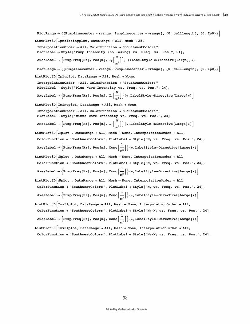
PlotRange ® 88Pumplinecenter - Νrange, Pumplinecenter + Νrange<, 80, celllength<, 80, Ip0<<FListPlot3DBIpnolasingplot, DataRange ® All, Mesh ® 25,
InterpolationOrder ® All, ColorFunction ® "SouthwestColors",
PlotLabel ® Style@"Pump Intensity Hno lasingL vs. Freq. vs. Pos.", 24D,
AxesLabel ® :Pump Freq@HzD, Pos@mD, IpBW
m2F>, H*LabelStyle®Directive@LargeD,*L
PlotRange ® 88Pumplinecenter - Νrange, Pumplinecenter + Νrange<, 80, celllength<, 80, Ip0<<FListPlot3DBIpluplot, DataRange ® All, Mesh ® None,
InterpolationOrder ® All, ColorFunction ® "SouthwestColors",
PlotLabel ® Style@"Plus Wave Intensity vs. Freq. vs. Pos.", 24D,
AxesLabel ® :Pump Freq@HzD, Pos@mD, I+BW
m2F>H*,LabelStyle®Directive@LargeD*LF
ListPlot3DBIminuplot, DataRange ® All, Mesh ® None,
InterpolationOrder ® All, ColorFunction ® "SouthwestColors",
PlotLabel ® Style@"Minus Wave Intensity vs. Freq. vs. Pos.", 24D,
AxesLabel ® :Pump Freq@HzD, Pos@mD, I-BW
m2F>H*,LabelStyle®Directive@LargeD*LF
ListPlot3DBN1plot , DataRange ® All, Mesh ® None, InterpolationOrder ® All,
ColorFunction ® "SouthwestColors", PlotLabel ® Style@"N1 vs. Freq. vs. Pos.", 24D,
AxesLabel ® :Pump Freq@HzD, Pos@mD, ConcB1
m3F>H*,LabelStyle®Directive@LargeD*LF
ListPlot3DBN2plot , DataRange ® All, Mesh ® None, InterpolationOrder ® All,
ColorFunction ® "SouthwestColors", PlotLabel ® Style@"N2 vs. Freq. vs. Pos.", 24D,
AxesLabel ® :Pump Freq@HzD, Pos@mD, ConcB1
m3F>H*,LabelStyle®Directive@LargeD*LF
ListPlot3DBN3plot , DataRange ® All, Mesh ® None, InterpolationOrder ® All,
ColorFunction ® "SouthwestColors", PlotLabel ® Style@"N3 vs. Freq. vs. Pos.", 24D,
AxesLabel ® :Pump Freq@HzD, Pos@mD, ConcB1
m3F>H*,LabelStyle®Directive@LargeD*LF
ListPlot3DBInv31plot, DataRange ® All, Mesh ® None, InterpolationOrder ® All,
ColorFunction ® "SouthwestColors", PlotLabel ® Style@"N3-N1 vs. Freq. vs. Pos.", 24D,
AxesLabel ® :Pump Freq@HzD, Pos@mD, ConcB1
m3F>H*,LabelStyle®Directive@LargeD*LF
ListPlot3DBInv21plot, DataRange ® All, Mesh ® None, InterpolationOrder ® All,
ColorFunction ® "SouthwestColors", PlotLabel ® Style@"N2-N1 vs. Freq. vs. Pos.", 24D,
ThreelevelCWModelNDSOLVEgapproxEqnsLoopedShootingNDsolveWorkingLasingRigrodtexapp.nb 29
Printed by Mathematica for Students
93

AxesLabel ® :Pump Freq@HzD, Pos@mD, ConcB1
m3F>H*,
PlotRange®9Automatic,Automatic,9-1017,1017==*LH*,LabelStyle®Directive@LargeD*LFListPlot3D@8Γplot, Αplot<, DataRange ® All, Mesh ® None, ColorFunction ® "SouthwestColors",
InterpolationOrder ® All, PlotLabel ® Style@"Gain Coeffcient vs. Freq. vs. Pos.", 24D,AxesLabel ® 8Pump Freq@HzD, Pos@mD, Γ<,PlotRange ® 88Pumplinecenter - Νrange, Pumplinecenter + Νrange<, 80, celllength<, 8-2 Α, 2 Α<<H*,LabelStyle®Directive@LargeD*LD
ListLinePlot@8Γofzplot<, PlotLabel ® Style@"Γ HIntegratedL vs. Pos", 24D,AxesLabel ® 8Pos@mD, Γ<H*,LabelStyle®Directive@LargeD*LD
ListLinePlotB8Ipluofzplot, Iminuofzplot<,PlotLabel ® StyleA"I+ and I-HIntegrated over ΝpL vs. Pos", 24E,
AxesLabel ® :Pos@mD, IBW
m2F>H*,LabelStyle®Directive@LargeD*LF
ListLinePlotBIlaseoutplot, PlotLabel ® Style@"Laser Output Intensity", 24D,
AxesLabel ® :Pump Freq@HzD, IoutBW
m2F>H*,LabelStyle®Directive@LargeD*LF
30 ThreelevelCWModelNDSOLVEgapproxEqnsLoopedShootingNDsolveWorkingLasingRigrodtexapp.nb
Printed by Mathematica for Students
94

H. Laser Output Power and Other System Outputs
Laseroutfunc = Interpolation@IlaseoutplotD;Plot@Laseroutfunc@ΝD * gIp0@ΝD, 8Ν, Pumplinecenter - Νrange, Pumplinecenter + Νrange<D;LasPower = NIntegrate@Laseroutfunc@ΝD * gIp0@ΝD,
8Ν, Pumplinecenter - Νrange, Pumplinecenter + Νrange<D;Γofzint = Interpolation@ΓofzplotD;
Γtotal =1
zfinal - znotNIntegrate@Γofzint@zD, 8z, znot, zfinal<D;
OutputEfficiency = LasPower � Ip0;
H*Interpolation@ ΓplotDIf@Γabove1==1,Γgain=NIntegrate@
NIntegrate@Interpolation@ ΓplotD*gIp0@ΝD,8Ν,Min@ΝΓarray @Νpumpcountg ,zcountgDD,Max@ΝΓarray @Νpumpcountg ,zcountgDD<D,8z,znot,zfinal<DD;*L
PrintAStyle@"1. The Output Laser Intensity of DPAL System Tested is predicted to be ",
30, BoldD, Style@LasPower, 30, Bold, RedD, StyleA"W�m2", 30, Bold, RedEEPrint@Style@"2. The Output Lasing Frequency of DPAL System Tested is predicted to be ",
30, BoldD, Style@Νlaser, 30, Bold, RedD, Style@"Hz", 30, Bold, RedDDPrint@Style@"3. The Output Efficiency of the Tested DPAL System is predicted to be ",
30, BoldD, Style@OutputEfficiency * 100, 30, Bold, RedD, Style@"%", 30, Bold, RedDDPrintAStyleA"4. Ip0�Isat for this system is ", 30, BoldE,Style@Ip0 � Isat@PumplinecenterD, 30, Bold, RedDE
Print@Style@"5. ΓHtotalL�Α or Gain Divded by Loss for this system is ", 30, BoldD,Style@Γtotal � Α, 30, Bold, RedDDH*This is a measure of the accuracy of the simulation*L
Print@Style@"6. The degree to which the boudary condition at z final was met was: ",
30, BoldD, Style@Rootfindavg, 30, Bold, RedDDH*,
"Note The smaller this number is the better. Above 1 is bad and implies
a solution set should be rerun with a longer�shorter cavity. "*LH*This is a measure of the accuracy of the simulation*L
ThreelevelCWModelNDSOLVEgapproxEqnsLoopedShootingNDsolveWorkingLasingRigrodtexapp.nb 31
Printed by Mathematica for Students
95

1. The Output Laser Intensityof DPAL System Tested is
predicted to be 358130.W�m22. The Output Lasing Frequencyof DPAL System Tested is
predicted to be 3.77109´1014Hz3. The Output Efficiencyof the Tested DPAL Systemis predicted to be 0.71626%
4. Ip0�Isat for this system is103.7825. ΓHtotalL�Α or Gain Divded byLoss for this system is 154.126
6. The degree to whichthe boudary condition at zfinal was met was: 1.66422
32 ThreelevelCWModelNDSOLVEgapproxEqnsLoopedShootingNDsolveWorkingLasingRigrodtexapp.nb
Printed by Mathematica for Students
96
Bibliography
[1] Beach R.J., V.K. Kanz S.A. Payne M.A. Dubinski, W.F. Krupke and L.D.Merkle. Opt Soc Am B, 21, 2004.
[2] Hager, Gordon D. “A Three Level Analytic Model for Alkali Metal VaporLasers”. Air Force Institute of Technology, Draft Aug 2008.
[3] Hager, Gordon D. “A quasi-two level analytic model for end pumped alkali metalvapor lasers”. Air Force Institute of Technology, Draft May 2008.
[4] Krupke W.F., V.K. Kanz, R.J. Beach and S.A. Payne. Opt Lett, 28, 2003.
[5] Lewis, Charlton D. “A theoretical model analysis of absorption of a three leveldiode pumped alkali laser”. Air Force Institute of Technology (Thesis), 2009.
[6] Readle J.D., J.T. Verdeyen T.M. Spinka D.L. Carroll, C.J. Wagner and J.G.Eden. “Pumping of atomic alkali lasers by photoexicitation of a resonance lineblue satellite and alkali-rare gas excimer dissociation”. Applied Physics Letters,94, 2009.
[7] Thompson, W.J. “Numerous neat algorithms for the voigt profile function”.Computers in Physics, 7, 1993.
[8] Verdeyen, Joseph T. Laser Electronics. Prentice Hall, 2002.
[9] Zhdanov, B.V. Opt Lett, 33, 2008.
[10] Zhdanov B.V., R.J. Knize. Opt Lett, 32, 2007.
97

REPORT DOCUMENTATION PAGE Form ApprovedOMB No. 0704–0188
The public reporting burden for this collection of information is estimated to average 1 hour per response, including the time for reviewing instructions, searching existing data sources, gathering andmaintaining the data needed, and completing and reviewing the collection of information. Send comments regarding this burden estimate or any other aspect of this collection of information, includingsuggestions for reducing this burden to Department of Defense, Washington Headquarters Services, Directorate for Information Operations and Reports (0704–0188), 1215 Jefferson Davis Highway,Suite 1204, Arlington, VA 22202–4302. Respondents should be aware that notwithstanding any other provision of law, no person shall be subject to any penalty for failing to comply with a collectionof information if it does not display a currently valid OMB control number. PLEASE DO NOT RETURN YOUR FORM TO THE ABOVE ADDRESS.
1. REPORT DATE (DD–MM–YYYY) 2. REPORT TYPE 3. DATES COVERED (From — To)
4. TITLE AND SUBTITLE 5a. CONTRACT NUMBER
5b. GRANT NUMBER
5c. PROGRAM ELEMENT NUMBER
5d. PROJECT NUMBER
5e. TASK NUMBER
5f. WORK UNIT NUMBER
6. AUTHOR(S)
7. PERFORMING ORGANIZATION NAME(S) AND ADDRESS(ES) 8. PERFORMING ORGANIZATION REPORTNUMBER
9. SPONSORING / MONITORING AGENCY NAME(S) AND ADDRESS(ES) 10. SPONSOR/MONITOR’S ACRONYM(S)
11. SPONSOR/MONITOR’S REPORTNUMBER(S)
12. DISTRIBUTION / AVAILABILITY STATEMENT
13. SUPPLEMENTARY NOTES
14. ABSTRACT
15. SUBJECT TERMS
16. SECURITY CLASSIFICATION OF:
a. REPORT b. ABSTRACT c. THIS PAGE
17. LIMITATION OFABSTRACT
18. NUMBEROFPAGES
19a. NAME OF RESPONSIBLE PERSON
19b. TELEPHONE NUMBER (include area code)
Standard Form 298 (Rev. 8–98)Prescribed by ANSI Std. Z39.18
27–03–2010 Master’s Thesis Aug 2008 — Mar 2010
Simulation of a Diode Pumped Alkali Laser, A Three Level NumericalApproach
Hackett, Shawn W. , 2Lt., USAF
Air Force Institute of TechnologyGraduate School of Engineering and Management (AFIT/EN)2950 Hobson WayWPAFB OH 45433-7765
AFIT/GAP/ENP/10-M06
HEL-JTO901 University Blvd SE Ste 100Albuquerque, NM 87106505-248-8200 ,[email protected]
HEL-JTO
APPROVED FOR PUBLIC RELEASE; DISTRIBUTION UNLIMITED.
This paper develops a three level model for a continuous wave diode pumped alkali laser by creating rate equations basedon a three level system. Differential equations for intra-gain pump attenuation and intra-gain laser growth are developedin the fashion done by Rigrod. Using Mathematica 7.0, these differential equations are solved numerically and a diodepumped alkali laser system is simulated.The results of the simulation are compared to previous experimental results andto previous computational results for similar systems. The absorption profile for the three level numerical model is shownto have excellent agreement with previous absorption models. The lineshapes of the three level numerical model arefound to be nearly identical to previous developments excepting those models assumptions. The three level numericalmodel provides results closer to experimental results than previous systems and provides results which observe effects notpreviously modeled, such as the effects of lasing on pump attenuation.
Diode Pumped Alkali Laser, Numerical Modelling, Rate Equation Analysis, Three Level Systems
U U U UU 111
LtCol. Jeremy C. Holtgrave
(937) 255-3636; [email protected]