AIDA’01-1

Applying the Hidden Markov Model Applying the Hidden Markov Model Methodology for Unsupervised Methodology for Unsupervised

Learning of Temporal DataLearning of Temporal Data

Cen Li1 and Gautam Biswas2

1Department of Computer Science

Middle Tennessee State University

2Department of EECS

Vanderbilt University

Nashville, TN 37235. USA.biswas@vuse.vanderbilt.edu

biswas@http://www.vuse.vanderbilt.edu/~biswas

June 21, 2001

AIDA’01-2

Problem DescriptionProblem Description Most real world systems are dynamic, e.g.,

Physical plants and Engineering systems Human Physiology Economic systemsSystems are complex: hard to understand, model, and analyzeBut our ability to collect data on these systems has increased

tremendously

Task: Use data to automatically build models, extend incomplete models, and verify and validate existing models using the data available.

Why models? Formal, abstract representation of phenomena or process Enables systematic analysis and predictionOur goal:

Build models, i.e., create structure from data using exploratory techniques

Challenge:Systematic and useful clustering algorithms for temporal data

AIDA’01-3

Outline of TalkOutline of Talk

Example Problem Related work on temporal data clustering Motivation for using Hidden Markov Model (HMM)

representation Bayesian HMM clustering methodology Experimental results

Synthetic Data Real world ecological data

Conclusions and future work

AIDA’01-4

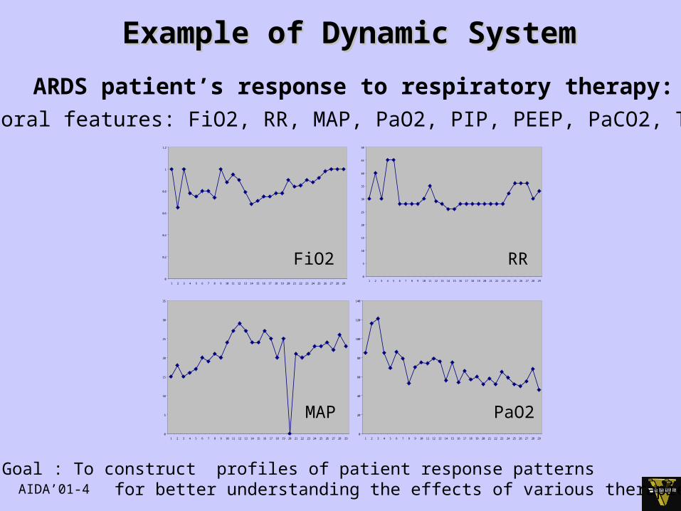
Example of Dynamic SystemExample of Dynamic System

0

0.2

0.4

0.6

0.8

1

1.2

1 2 3 4 5 6 7 8 9 10 11 12 13 14 15 16 17 18 19 20 21 22 23 24 25 26 27 28 29

0

5

10

15

20

25

30

35

40

45

50

1 2 3 4 5 6 7 8 9 10 11 12 13 14 15 16 17 18 19 20 21 22 23 24 25 26 27 28 29

0

5

10

15

20

25

30

35

1 2 3 4 5 6 7 8 9 10 11 12 13 14 15 16 17 18 19 20 21 22 23 24 25 26 27 28 29

0

20

40

60

80

100

120

140

1 2 3 4 5 6 7 8 9 10 11 12 13 14 15 16 17 18 19 20 21 22 23 24 25 26 27 28 29

FiO2 RR

MAP PaO2

Temporal features: FiO2, RR, MAP, PaO2, PIP, PEEP, PaCO2, TV ...

ARDS patient’s response to respiratory therapy:

Goal : To construct profiles of patient response patterns for better understanding the effects of various therapies

AIDA’01-5

Problem DescriptionProblem Description

Unsupervised Classification (Clustering)Given data objects described by multiple temporal features:

(1) to assign category information to individual objects by objectively partitioning the objects into homogeneous groups such that the within group object similarity and the between group object dissimilarity are maximized,

(2) to form succinct description for each category derived.

Clustering System

1

2

K

O , O , ... O 1 2 N

Data: Cluster 2

Cluster 1

Cluster K

AIDA’01-7

Motivation for using HMM RepresentationMotivation for using HMM Representation What are our modeling objectives ? Why do we choose the HMM representation ?

The hidden states valid stages of a dynamic process Direct probabilistic links probabilistic transitions among

different stages

S S

S

S

S S

a 00

a

a

a

a

a

a a a

a a

a

a

11 22

33

55

44

40

01 12 25

32 23

24

0

b = N( , )

b =N( , )

b =N( , )

b =N( , )

b =N( , ) b =N( , )

0

0 1

4

5 2

3

0

1

2

3

4

5

0 0

1 1 1

4 4 4

5 5 5

2 2 2

3 3 3

S = Unstable S = Weaning ready S = Active weaning S = No progress S = More dependent S = Successful completion

Example HMM for the Therapy Response Data

Mathematically HMM Model made up of three components

1. : initial state probabilities 2. A: transition matrix3. B: emission matrix ),( N

AIDA’01-8

Continuous Speech SignalContinuous Speech Signal

Rabiner and Huang, 1993

Spectral sequence feature extraction statistical pattern recognition

Isolated Word Recognition1 HMM per word2-10 states per HMMdirect continuous density HMMsproduce best results

Continuous Word RecognitionNumber of words (?) Utterance boundaries (?)Word boundaries: fuzzy/non uniqueMatching word reference patterns to Words: exponential problem

Whole word models typically not used for continuous speech recognition

AIDA’01-9

Continuous Speech RecognizerContinuous Speech Recognizerusing sub-wordsusing sub-words

Recognized

Sentence

SpectralAnalysis

Speech

Input

Word-levelMatch

Sentence-levelMatch

Word ModelComposition

SubwordModels

Lexicon Grammar Semantics

WordModel

LanguageModel

Sentence (Sw):

W1 W2

silence silence

Word (W1):U1(W1) U2(W1) UL(W1)(W1)

Sub-word Unit (PLU):

Rabiner and Huang, 1993

AIDA’01-10

Continuous Speech RecognitionContinuous Speech Recognition

CharacteristicsCharacteristics

Lot of background knowledge available, e.g., Phonemes & syllables for isolated word recognition Sub-word units (Phonelike units (PLUs), Syllable-like units,

Acoustic units) for word segmentation Grammar and semantics for language models

As a result, HMM structure usually well-defined Recognition task dependent on learning model parameters Clustering techniques employed to derive efficient state

representation Single speaker versus speaker independent recognition

Question: What about domains where structure not well known & Data not as well-defined

AIDA’01-11

Past Work on HMM ClusteringPast Work on HMM Clustering

Past Work: [Rabiner et al., 1989]

HMM Likelihood Clustering, HMM Threshold Clustering – Baum Welch, Viterbi methods for parameter estimation

[Lee, 1990] Agglomerative procedure

[Bahl et al., 1986], [Normandin et al., 1994] HMM parameter estimation by Maximal Mutual Information (MMI)

[Kosaka et al. 1995] HMnet composition and clustering (CCL); Bhattacharyya distance measure

[Dermatas & Kokkinakis, 1996] Extended Rabiner et al.’s work – more sophisticated clustering structure –

clustering by recognition error [Smyth, 1997]

Clustering with finite mixture models

Limitations: No objective criterion for cluster partition evaluation and selection Apply uniform, pre-defined HMM model size for clustering

App

lied

to S

peec

h R

ecog

nitio

n

AIDA’01-12

Original work on HMM parameter Original work on HMM parameter estimation (Rabiner, et al., 1989)estimation (Rabiner, et al., 1989)

Maximum Likelihood Method (Baum Welch): Parameter estimation by the E(xpectation)-M(aximization)

method Assign initial parameters E-step: compute expected values of the necessary

statistics M-step: update model parameter values to maximize

likelihoodUse forward-backward procedure to cut down on the

computational requirements.Baum Welch method very sensitive to initialization: use

Viterbi method to find most likely path, and use that to initialize parameters.

Extensions to method (estimate model size): state splitting, state merging, etc.

AIDA’01-13

S S

S

S

S S

a 00

a

a

a

a

a

a a a

a a

a

a

11 22

33

55

44

40

01 12 25

32 23

24

0

b = N( , )

b =N( , )

b =N( , )

b =N( , )

b =N( , ) b =N( , )

0

0 1

4

5 2

3

0

1

2

3

4

5

0 0

1 1 1

4 4 4

5 5 5

2 2 2

3 3 3

S = Unstable S = Weaning ready S = Active weaning S = No progress S = More dependent S = Successful completion

Example HMM for the Therapy Response Data

AIDA’01-14

Our Approach to HMM ClusteringOur Approach to HMM Clustering

Four nested search loops:

Loop 1: search for the optimal number of clusters in

the partition,

Loop 2: search for the optimal object distribution to

the clusters in the partition,

Loop 3: search for the optimal HMM model size

for each cluster in the partition, and

Loop 4: search for the optimal model parameter configuration for each model .

Search space:

N

i

i

j

j

k

LN

pj

Nj

LNO1 1 1 1

)(

HMMLearning

AIDA’01-15

Introducing Heuristics to HMM ClusteringIntroducing Heuristics to HMM Clustering Four nested levels of search:

Loop 1: search for the optimal number of clusters in the

partition,

Loop 2: search for the optimal object distribution to clusters in

the partition,

Loop 3: search for the optimal HMM model size for each

cluster in the partition, and

Loop 4: search for the optimal model parameter configuration

for each model .

Bayesian Model

Selection

HMM Learning

AIDA’01-16

Bayesian Model SelectionBayesian Model Selection

)|(

)(

)()|()|(

MDP

DP

MPMDPDMP

dMPMDP )|(),|(

(Marginal Likelihood)

Model PosteriorProbability:

Goal: Select Model M that maximizes P(M|D)

AIDA’01-17

Computing Marginal LikelihhodsComputing Marginal Likelihhods

Issue of complete versus incomplete data

Approximation Techniques Monte Carlo methods (Gibbs sampling) Candidate Method (variation of Gibbs sampling) – Chickering Laplace approximation (multivariate Gaussian, quadratic

Taylor series approx.)

Bayesian Information Criteria – derived from Laplace approx.

Very efficient

Cheeseman-Stutz approx.

AIDA’01-18

)|ˆ(log)ˆ,|(log)|(log MPMDPMDP

Marginal Likelihood ApproximationsMarginal Likelihood Approximations

Bayesian Information Criterion (BIC):

Cheeseman-Stutz (CS) Approximation:

)log2

()ˆ,|(log)|(log Nd

MDPDMP

Likelihood Model Complexity Penalty

Likelihood Model Prior Probability

NdD kk

kkj

kj

NP

k

log2

),|(log ˆ1

AIDA’01-20

Bayesian Model Selection for Bayesian Model Selection for HMM Model Size SelectionHMM Model Size Selection

Goal: To select the optimal number of states, K, for a HMM that maximizes

S SS

k

1 2 K

)|( DkKP

AIDA’01-21

BIC and CS for HMM Model Size SelectionBIC and CS for HMM Model Size Selection

-900

-800

-700

-600

-500

-400

-300

-200

-100

0

100

-1000

-900

-800

-700

-600

-500

-400

-300

-200

-100

0

(b) CS Approximation

likelihood

(a) BIC approximation

CS

prior

-1000

-900

-800

-700

-600

-500

-400

-300

-200

-100

0

Model size

-920

-910

-900

-890

-880

-870

-860

-850

-840

-830

-820

penalty

likelihood

BIC

2 3 4 5 6 7 8 9 102 3 4 5 6 7 8 9 10

AIDA’01-22

HMM Model Size Selection ProcessHMM Model Size Selection Process

Sequential search for HMM model size with a heuristic stopping criterion -- Bayesian model selection criterion approximated by BIC and CS

Issue 2: State initialization by K-means clustering

Initial 1-state HMM

Increase HMM size by 1 state

Learn HMM Parameter

Configuration

HMM Score

Increases?

yes

no

Accept the previous HMM

Assumptions:Data Complete Data Sufficient – otherwise, suboptimal structure

AIDA’01-24

Cluster Partition Selection :Cluster Partition Selection : Bayesian Model Selection for Mixture of HMMs Bayesian Model Selection for Mixture of HMMs

C

1 2 K

M:

P P P 1 K

c=1 c=K c=2

2

Goal: Select partition with the optimal number of clusters, K, that maximizes P(M|D)

Partition Posterior Probability (PPP), ),ˆ|()|()|( MDPMDPDMP

),,|( ˆ11

kkkii

K

kk

N

iddP f

Apply BIC approximation

AIDA’01-25

BIC and CS for Cluster Partition SelectionBIC and CS for Cluster Partition Selection

-150000

-145000

-140000

-135000

-130000

-125000

-120000

1 2 3 4 5 6 7 8 9 10

-1200

-1000

-800

-600

-400

-200

0

-150000

-145000

-140000

-135000

-130000

-125000

-120000

1 2 3 4 5 6 7 8 9 10

-1800

-1600

-1400

-1200

-1000

-800

-600

-400

-200

0

(a) BIC approximation (b) CS approximation

penalty prior

likelihood likelihood

BICCS

1 2 3 4 5 6 7 8 9 10 1 2 3 4 5 6 7 8 9 10

AIDA’01-26

Bayesian Model Selection for Partition Bayesian Model Selection for Partition Evaluation and SelectionEvaluation and Selection

Sequential search for clustering partition model using a heuristic stopping criterion -- Bayesian model selection criterion (approximated by BIC and CS)

Initial Partition of size 1

Partition Expansion

Fixed size partition formaton

Partition Score

Increases?

yes

no

Accept the previous partition

AIDA’01-27

Fixed Size Cluster Partition FormationFixed Size Cluster Partition Formation

Partition model

converges ?

Update Models

C C C C 1 3 2 K

Assign N objects to the K clusters

yes

no

Accept the partition

Goal : to maximize:

),ˆ|(log log

),ˆ|(log

),ˆ|(log

),ˆ|(log

1 11 1

1 1

1

kki

K

k

N

i

N

i

K

kik

kki

N

i

K

kik

N

ii

xf w

xfw

MxP

MXP

Hard Data Partitioning

BIC criteriaNK

K

kkd

log2

1

AIDA’01-28

Introducing Heuristics to HMM ClusteringIntroducing Heuristics to HMM Clustering Four nested levels of search:

Step 1: search for the optimal number of clusters in the

partition,

Step 2: search for the optimal object distribution to clusters in

the partition,

Step 3: search for the optimal HMM model size for each

cluster in the partition, and

Step 4: search for the optimal model parameter configuration

for each model .

Bayesian Model

Selection

EM with hard data

partitioning& heuristic

modelinitialization

Clustering HMM

initialization

AIDA’01-29

Bayesian HMM Clustering (BHMMC) with Bayesian HMM Clustering (BHMMC) with Component Model Size SelectionComponent Model Size Selection

K=1 Select K seeds

HMM model size

selection

Object to cluster

distribution

Member-ship

change?

HMM parameter

reestimation

Partition score

increase?

K=K+1

yes

yes

no

no

Accept previous partition as final partition

HMM size selection

(all clusters)

Complexity O(KNMmaxL)

AIDA’01-30

ExperimentsExperiments

Exp 1: Study the HMM model size selection method

Exp 2: Compare HMM clustering with varying HMM sizes vs. HMM clustering with fixed HMM

Exp 3: Clustering robustness to data skewness

Exp 4: Clustering sensitivity to seed selection

AIDA’01-31

Experiment 1: Modeling with HMMExperiment 1: Modeling with HMM

2

3

4

5

6

7

8

9

10

1

1 2 3 4 5 6 7 8 9 10 11 12 13 14 X

Y y=k'x+b', k'= -1/k

S1

3S

2S

S4

y=kx+b

S m3 m 11 2

4 m

d(S , S )=g( )

d(S , S )=g'( )

d(S , S ) = f( )

AIDA’01-32

Experiment 1: Modeling with HMM Experiment 1: Modeling with HMM (continued)(continued)

2.2

2.4

2.6

2.8

3

3.2

3.4

3.6

3.8

4

4.2

HMM model sizes rediscovered given 4-state HMMs of different 1and 2 values: mean

=0.5

HMM SizeRediscovered

23 2 1 0.5 0.1

= 1

= 3

= 2

1

1

1

1

AIDA’01-33

Experiment 2: Clustering with varying Experiment 2: Clustering with varying vs.vs. fixed HMM model sizefixed HMM model size

CLUSTERING WITH FIXED SIZE HMMCRITERIONFUNCTION 3 8 15

CLUSTERINGWITH VARYING

SIZE HMM

BIC 48(24) 26(27) 70(22) 0(0)

CS 26(27) 24(29) 84(29) 0(0)

Partition Misclassification Count: mean (standard deviation)

AIDA’01-34

Experiment 2 (continued)Experiment 2 (continued)

-2000.00

-1950.00

-1900.00

-1850.00

-1800.00

-1750.00

-1700.00

-1650.00

-1600.00

-1550.00

-1500.001 2 3 4 5

Between Partition Similarity

Varying

Fixed 3

Fixed 8

Fixed 15

AIDA’01-35

-230000

-220000

-210000

-200000

-190000

-180000

-1700001 2 3 4 5

Experiment 2 (continued)Experiment 2 (continued)

Varying

Fixed 3

Fixed 8

Fixed 15

Partition Posterior Probability

AIDA’01-36

Experiment 3: Experiment 3: BHMMC with regular vs. skewed dataBHMMC with regular vs. skewed data

0

1

2

3

4

5

6

5-95% 10-90% 20-80% 30-70% 40-60% 50-50%

Average Misclassification Count

Cluster 1 - Cluster 2 %

Model distance = level 1

Model distance = level 2

AIDA’01-37

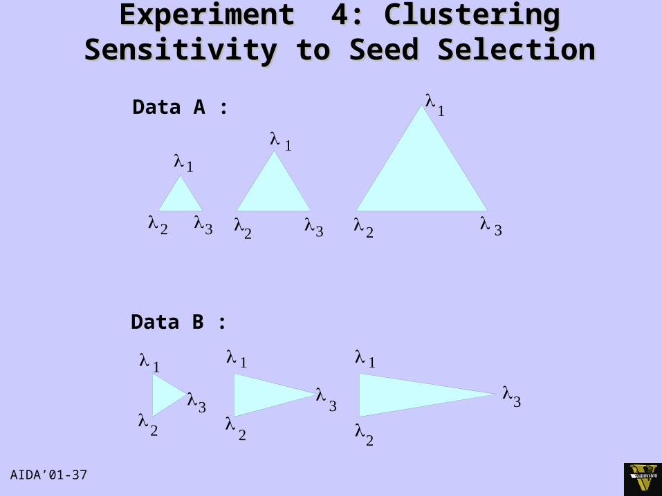
Experiment 4: Clustering Sensitivity to Experiment 4: Clustering Sensitivity to Seed SelectionSeed Selection

111

Data B :

11

1

Data A :

AIDA’01-38

Experiment 4 (continued)Experiment 4 (continued)

0

5

10

15

20

25

30

0

50

100

150

200

250

300

350

400

450

Data B Data B

Data A

Data A

1 2 3 1 2 3

Average over 10 runs

Variance on PPP(mean)Variance on misclassification count (mean)

Level Level

AIDA’01-39

Experiments with Ecological DataExperiments with Ecological Data

collaborators: Dr. Mike Dale and Dr. Pat Dalecollaborators: Dr. Mike Dale and Dr. Pat DaleSchool of Environmental Studies, Griffith University, AustraliaSchool of Environmental Studies, Griffith University, Australia

Study the ecological effects of mosquito control by runnelingrunneling, i.e., changing the drainage patterns in an area

Data collected from about 30 sites30 sites in a salt marsh area south of Brisbane, Australia

Data: At each site we have four measures of species performance Height and density of the grass Sporobolous (marine couch) Height and density of succulent Sarcocornia (samphire) 11 other environmental variables measured (they have missing

values), but they were not used for cluster generation.

Data collected in 3 month intervals3 month intervals starting mid 1985, each temporal data sequence is 56 long56 long

AIDA’01-40

Results of Experiments (1)Results of Experiments (1)

Experiment 1: Generate HMM Clusters with all four plant variables. Result: Single dynamic process (one cluster

partition) with 4 states that form a cycle.

SporobolousDense & TallSarcocornia

Sparse

SporobolousSparse & Moderate

SarcocorniaShort & Sparse

SporobolousSparse

SarcocorniaSparse & Tall

SporobolousAlmost absentSarcocornia

Dense & Moderate

Conclusions: Mosquito control treatment has no significant effects on plant ecologyConclusions: Mosquito control treatment has no significant effects on plant ecology

Some parts of the marsh shifted – got wetter, and shifted more toward Some parts of the marsh shifted – got wetter, and shifted more toward SarcocorniaSarcocornia

AIDA’01-41

Results of Experiments (2)Results of Experiments (2) Experiment 2: Isolate and study the effects on the Sporobolous plant

Result: Two cluster partition: Cluster 1: 5 states with low transition probabilities (more or less static)

Cluster 2: Two interacting dynamic cyclesS1

SporobolousDense & Tall

S5Sporobolous

Short & Dense

S2Sporobolous

Medium & Dense

S3Sporobolous

Sparse & Medium

S4SporobolousAlmost Bare

0.9

0.9

0.45

0.33

0.5

0.330.330.9

0.1

Loop 1

Loop 2

AIDA’01-42

Results of Experiments (3)Results of Experiments (3)

Summary of Results (Experiment 2) Two paths for getting Sporobolous to bare ground

In loop 1 the grass recovers through state 2 In loop 2 the process may stay in state 3 (medium height) with

equal chance of going bare (state 4) or becoming short and dense (state 5).

Shows modifications (new states) to the overall process Other observations

Usually ecological systems have more memory than 3 months. May require higher order Markov processes

Feature values may not be independent (consequences?) There was a drought in the middle of the observation period Amount of data available for parameter estimation limited – may affect

statistical validity of estimated parameters How do we incorporate the environmental variables into model? Some

are discrete. They are at a different temporal granularity. Missing values.

AIDA’01-44

Future WorkFuture Work

Improve clustering stability Evaluate partition quality in terms of the predictiveness of the cluster models Investigate incremental Bayesian HMM clustering approaches Enhance HMM of dynamic processes (higher order models, non stationary

processes) Apply this methodology to real data, perform knowledge based model

interpretation and analysis Ecological data Stock data Therapy response data