aiaa 2012-0557 numerical simulation of a tornado generating … · 2013-04-10 · aiaa 2012-0557 ....

AIAA 2012-0557 Numerical Simulation of a Tornado Generating Supercell Fred H. Proctor and Nash’at N. Ahmad NASA Langley Research Center Hampton, VA and Fanny M. Limon Duparcmeur Metis Technology Solutions Hampton, VA

50th AIAA Aerospace Sciences Meeting 9-12 January 2012 / Nashville, TN

This material is declared a work of the U.S. Government.

https://ntrs.nasa.gov/search.jsp?R=20120001276 2020-05-23T19:34:16+00:00Z

American Institute of Aeronautics and Astronautics

1

Numerical Simulation of a Tornado Generating Supercell

Fred H. Proctor* and Nash’at N. Ahmad† NASA Langley Research Center, Hampton, VA 23681-2199

and

Fanny M. Limon Duparcmeur‡ Metis Tech. Solutions, Hampton, Virginia 23681-2199

The development of tornadoes from a tornado generating supercell is investigated with a large eddy simulation weather model. Numerical simulations are initialized with a sounding representing the environment of a tornado producing supercell that affected North Carolina and Virginia during the Spring of 2011. The structure of the simulated storm was very similar to that of a classic supercell, and compared favorably to the storm that affected the vicinity of Raleigh, North Carolina. The presence of mid-level moisture was found to be important in determining whether a supercell would generate tornadoes. The simulations generated multiple tornadoes, including cyclonic-anticyclonic pairs. The structure and the evolution of these tornadoes are examined during their lifecycle.

Nomenclature AGL = Above Ground Level dBZ = decibels of radar reflectivity, Z EPOT = Equivalent potential temperature NEXRAD = Next Generation Radar p = pressure deviation from ambient atmospheric pressure P = atmospheric pressure u = horizontal velocity component in the east direction v = horizontal velocity component in the north direction w = vertical component of velocity t = time coordinate x = Cartesian coordinate in east direction y = Cartesian coordinate in north direction z = Cartesian coordinate in vertical direction, altitude above ground Z = radar reflectivity factor (mm6 m-3) ΔP = maximum pressure deficit ∆x = grid size along x-coordinate (125m) ∆y = grid size along y-coordinate (125m) ∆z = grid size along z-coordinate (100m)

I. Introduction UPERCELL thunderstorms are of special concern to meteorologists since they are almost always associated with severe weather. Unlike other more common types of cumulonimbus convection, a supercell maintains a

powerful, quasi-steady, long-lived updraft.1 Supercell thunderstorms may generate damaging surface winds, hail, lightning, heavy rain, strong vertical air currents, and sometimes may spawn tornadoes. Supercell storms usually last for more than an hour, and have lateral scales of tens of kilometers. They may extend vertically through the troposphere, with tops sometimes overshooting into the lower stratosphere. Environmental conditions favoring the

* Senior Research Scientist, Crew Systems & Aviation Operations Branch, Mail Stop 152, AIAA Senior Member. † Research Aerospace Engineer, Crew Systems & Aviation Operations Branch, Mail Stop 152, AIAA Senior Member. ‡ Research Aerospace Engineer, NASA Contractor, Mail Stop 152, AIAA Member.

S


2

formation of supercells require strong vertical wind shear and convectively unstable lapse-rates for temperature. Regions favorable for supercell growth can be predicted with numerical weather forecast models and the actual storms can be identified and tracked in real-time using Doppler radar. Weather conditions associated with supercell storms can be destructive and can threaten the safety of the general public. These storms also can be a nuisance to air travel. Supercell storms may reduce the capacity of the National Airspace System by forcing delays and cancellations. For example, surface airport operations may be suspended during the passage of supercells due to the threat of high winds, lightning, poor visibility, and hail. Other hazards including the threat of turbulence, icing, and wind shear, can add to the safety concerns for flying aircraft and result in further delays and additional fuel costs.

The supercell representation proposed by Lemon and Doswell2 shows one main updraft region and two primary downdraft regions (Figure 1). The updraft is located on the rear flank and provides the warm moist low-level air that feeds the storm. The updraft extends to the top of the storm and can cause pulsing tops that overshoot above the cumulonimbus anvil. The storm updraft, once initiated, is not choked off by the storm’s rain cooled outflow and maintains the persistence of the supercell storm.3 This updraft may be associated with rotation and the development of a mesocyclone.4 The primary source for rotation within the mesocyclone is the vertical tilting of the horizontal vorticity associated with the environmental wind shear.5 Other updraft cells within the supercell complex can be triggered along the gust front boundary of the precipitation cooled outflow. New cells also may generate from the dynamic splitting of the main updraft.6 Primary downdraft regions are located in the forward region and on the rear flank. The forward downdraft is driven by evaporative cooling and maintains the cool outflow region under the storm. The rear flank downdraft is (partly) dynamically driven,7 and is instrumental in bringing vorticity from storm mid-levels to the surface.8,9 A radar hook echo appendage, located at the rear flank position, may be formed as precipitation is swept into the cyclonic wind circulation of the storm’s mesocyclone. Strong damaging winds and tornadoes are frequently associated with the mesocyclone. Thus, the hook echo has long been an identifying signature of the potential for tornadoes. Translation of a supercell storm tends to be slower and to the right of other nearby cells.

Figure 1. Schematic representation of supercell thunderstorm adapted from the conceptual model presented by Lemon and Doswell2. Dark shaded areas represent precipitation region, and thunderstorm outflow region indicated by barbed line. Also depicted are the locations of the forward flanking downdraft (FFD) and rear flanking downdraft (RFD), mesocyclone updraft (U) and typical location of tornado (T) if one occurs. From Shabbot and Markowski.10

A lowered cloud base, referred to as a wall cloud, may form underneath the updraft as some of the rain cooled air

is swept into the updraft. A tornado may appear to lower from the base of the wall cloud as its column of rotating air becomes tighter and the pressure deviation grows.11 The decrease in pressure reduces the temperature, causing condensation to occur in the funnel.12 Updrafts within the tornado may be enhanced by the reduction in tangential velocity near the ground due to surface friction.13 This causes strong pressure gradients which forces strong low-level inflow and upward motion within a tornado. Some supercells spawn families of tornadoes, while others may


3

produce long-lived tornadoes that have paths of hundreds of kilometers. A tornado lifecycle usually goes through a developing stage where the funnel descends downward as its rotating column of air intensifies. It may then connect to a debris cloud and widen as it continues to intensify. As the tornado goes through its decay stage, the funnel sometimes narrows and becomes tilted and rope-like before dissipating.14 Supercell storms can produce families of tornadoes, sometimes with both cyclonic and anticyclonic tornadoes in nearby proximity.15,16,17,18 Usually, the anticyclonic tornado is located to the right (relative to the motion of the supercell) of its companion cyclonic tornado.

Although tornadoes can be generated from nonsupercelluar convection, the vast majority of strong tornadoes are spawned from supercells.19 However, many supercells do not produce tornadoes,20,21 and our understanding of conditions that lead to tornadic supercells is inadequate. The dynamics of supercell storms are generally understood, but the conditions that lead to tornadogenesis are unclear. It is generally accepted that supercells acquire rotation at storm mid-levels via the tilting of horizontal vorticity associated with the vertical shear in the environment. When the horizontal vorticity is crosswise to the storm inflow, the updraft may acquire a couplet of positive and negative vertical vorticity. When the storm-relative winds veer with height in the lowest few kilometers, the horizontal vorticity may be oriented streamwise to the flow into the updraft, and the updraft may acquire either a net cyclonic or an anticyclonic rotation.22 Since rotation acquired from vortex tilting occurs in the rising updraft air, this process does not explain how rotation can arrive at the ground and fuel the development of a tornado. Numerical studies by Klemp and Rotunno,7 as well as Wicker and Wilhelmson,23 have reported that baroclinic generation of vorticity along the forward flank of the storm’s rain-cooled outflow is an important contribution for low-level rotation. However, Shabbott and Markowski10 have questioned the importance of this process, arguing that strong baroclinicity was not observed in a significant portion of the field measurements that they analyzed. Another source for low-level rotation is the downward transport and baroclinic generation of vorticity by the rear flanking downdraft.7,8,21,23,24 Pre-existing rotation aloft could maintain an upward pressure gradient force that is needed to recycle the more stable rain-cooled air, while maintaining convergence into the updraft. This process also could concentrate the low-level vorticity that is supplied by the flanking downdraft.

In order to investigate tornado generation by supercell storms, this study will use the Terminal Area Simulation System (TASS) which is a three-dimensional large eddy simulation cloud model. To best replicate a realistic event, the model is initialized with a modified sounding representing the environment associated with a major outbreak of supercell tornadoes. The case representing the input environment is described in Section 2, the numerical model and initial conditions are discussed in Section 3, results from the numerical simulations are described in Section 4, and a summary is provided in Section 5.

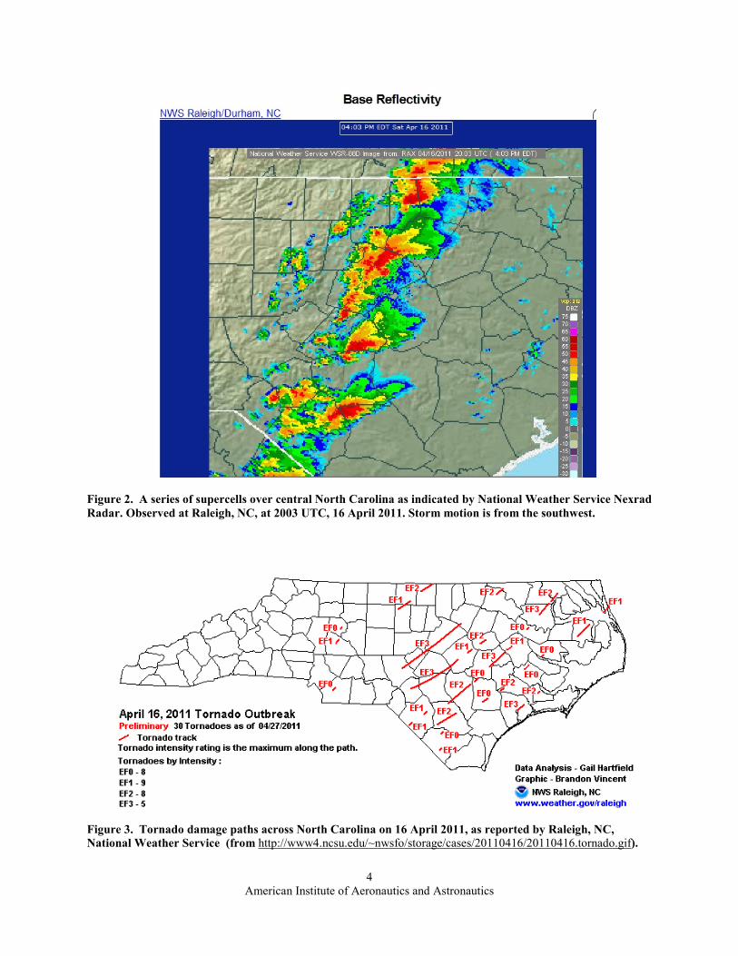
II. Atlantic States Tornado Outbreak of 2011 On the afternoon and evening of 16 April 2011, a series of supercell storms developed and moved across South

Carolina, North Carolina and Virginia, spawning over 40 tornadoes (e.g., Figures 2 - 5). One of the more notable tornadoes struck Raleigh, North Carolina, causing fatalities and severe structural damage. The supercell that produced this tornado developed in Moore County in central North Carolina, then traveled northeastward towards Raleigh, and later moved into southeastern Virginia. Additional fatalities resulted when a tornado from this same supercell moved through Gloucester, Virginia. Radar observation and accounts of this long-lived storm indicated that it was a supercell storm. The storm was associated with a radar hook echo and produced multiple tornadoes during its lifetime. The Raleigh tornado, spawned by this storm had a path length of 100km, damage consistent with an EF-3 rating,25 and a damage path as wide as 500m.26 The funnel’s visual appearance was described as a wedge that on occasion was wrapped within a rain curtain.

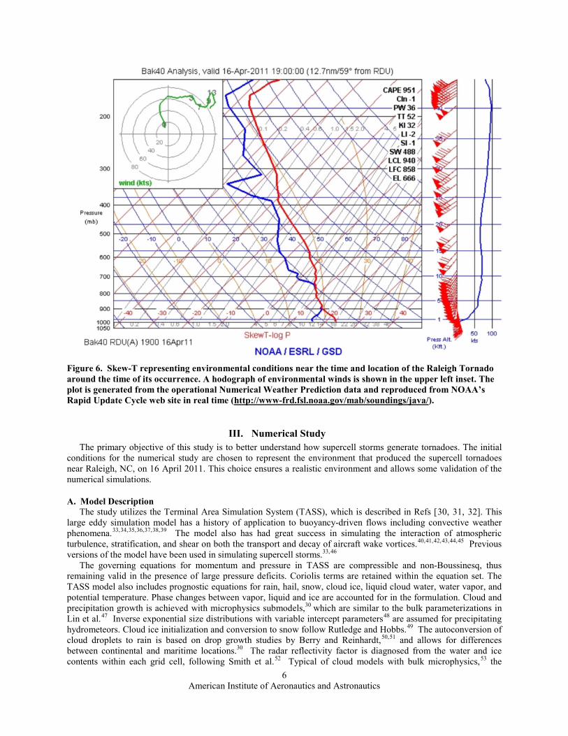
The National Oceanic and Atmospheric Administration’s (NOAA) numerical weather models predicted favorable conditions for the severe weather within the tornado outbreak area, including strong helicity27,28 and convective instability. A sounding from one of NOAA’s operational forecast models shows strong vertical shearing and veering of the low-level winds as well as moderate values of convective available potential energy29 (CAPE) (Figure 6). The severe weather potential was recognized by the National Weather Service (NWS), with tornado and severe weather watches issued for the region of the outbreak.


4

Figure 2. A series of supercells over central North Carolina as indicated by National Weather Service Nexrad Radar. Observed at Raleigh, NC, at 2003 UTC, 16 April 2011. Storm motion is from the southwest.

Figure 3. Tornado damage paths across North Carolina on 16 April 2011, as reported by Raleigh, NC, National Weather Service (from http://www4.ncsu.edu/~nwsfo/storage/cases/20110416/20110416.tornado.gif).

http://www4.ncsu.edu/~nwsfo/storage/cases/20110416/20110416.tornado.gif


5

Figure 4. Supercell with hook near Emporia, VA, as indicated by National Weather Service Nexrad Radar. Observed at Wakefield, VA, at 0152 UTC, 17 April 2011. Storm motion is from the southwest.

Figure 5. Tornado damage paths across southeast Virginia on 16-17 April 2011, as reported by Wakefield, Virginia, National Weather Service (from http://www.erh.noaa.gov/akq/wx_events/severe/apr_16_2011/April16_2011.png).

http://www.erh.noaa.gov/akq/wx_events/severe/apr_16_2011/April16_2011.png


6

Figure 6. Skew-T representing environmental conditions near the time and location of the Raleigh Tornado around the time of its occurrence. A hodograph of environmental winds is shown in the upper left inset. The plot is generated from the operational Numerical Weather Prediction data and reproduced from NOAA’s Rapid Update Cycle web site in real time (http://www-frd.fsl.noaa.gov/mab/soundings/java/).

III. Numerical Study The primary objective of this study is to better understand how supercell storms generate tornadoes. The initial

conditions for the numerical study are chosen to represent the environment that produced the supercell tornadoes near Raleigh, NC, on 16 April 2011. This choice ensures a realistic environment and allows some validation of the numerical simulations.

A. Model Description The study utilizes the Terminal Area Simulation System (TASS), which is described in Refs [30, 31, 32]. This

large eddy simulation model has a history of application to buoyancy-driven flows including convective weather phenomena.33,34,35,36,37,38,39 The model also has had great success in simulating the interaction of atmospheric turbulence, stratification, and shear on both the transport and decay of aircraft wake vortices.40,41,42,43,44,45 Previous versions of the model have been used in simulating supercell storms.33,46

The governing equations for momentum and pressure in TASS are compressible and non-Boussinesq, thus remaining valid in the presence of large pressure deficits. Coriolis terms are retained within the equation set. The TASS model also includes prognostic equations for rain, hail, snow, cloud ice, liquid cloud water, water vapor, and potential temperature. Phase changes between vapor, liquid and ice are accounted for in the formulation. Cloud and precipitation growth is achieved with microphysics submodels,30 which are similar to the bulk parameterizations in Lin et al.47 Inverse exponential size distributions with variable intercept parameters48 are assumed for precipitating hydrometeors. Cloud ice initialization and conversion to snow follow Rutledge and Hobbs.49 The autoconversion of cloud droplets to rain is based on drop growth studies by Berry and Reinhardt,50,51 and allows for differences between continental and maritime locations.30 The radar reflectivity factor is diagnosed from the water and ice contents within each grid cell, following Smith et al.52 Typical of cloud models with bulk microphysics,53 the

http://www-frd.fsl.noaa.gov/mab/soundings/java/


7

simulated radar reflectivity factors may be larger than observed, especially for deep convection within moist environments.39 Some discrepancy with observed radar reflectivity factor is expected, since the model does not take into account the radar beam size and geometry.

Since turbulence is strongly affected by the rotation of a swirling vortex, TASS uses a formulation that modulates the subgrid diffusion in rotating flow. This formulation was found necessary in the simulation of wake vortices to prevent unrealistic core growth.54 For subgrid turbulence, TASS uses either a conventional Smagorinsky55 model or a formulation proposed by Vreman.56 In this study, the Vreman formulation is used since it is insensitive to mean shear flow. The ground boundary is nonslip with a parameterization for surface stress based on Monin-Obukhov similarity theory.42 The surface boundary is assumed to be flat with a uniform surface roughness, z0, set to 30cm.

The TASS model equations are discretized using quadratic-conservative fourth-order finite-differences in space for the calculation of momentum and pressure fields.57 and the third-order upstream-biased Leonard scheme58 is used to calculate the transport of potential temperature and water vapor. A Monotone Upstream-centered Scheme for Conservation Laws (MUSCL)-type scheme after van Leer59,60 is used for the transport of water substance variables. The TASS computational mesh uses Arakawa C-grid staggering61 for specifying velocities and thermodynamic quantities. The Klemp-Wilhelmson time-splitting scheme62 is used for computational efficiency in which the higher-frequency terms are integrated by enforcing the CFL criteria to take into account sound wave propagation due to compressibility effects. The remaining terms are integrated using a larger time step that is appropriate for anelastic and incompressible flows.63 An Adams-Bashforth scheme is assumed for time differencing of momentum and pressure for both large and small time step approximations. Time steps are internally set and adjusted to meet numerical stability criteria. A sixth-order spatial filter is used to damp-out spurious oscillations in the velocity field that may arise due to the use of centered-differencing of momentum and pressure terms. Numerical tests have shown that the numerical formulation for the momentum and pressure equations in TASS are mass conservative and essentially free of numerical diffusion. Nonreflecting Orlanski boundary conditions64 are imposed on open/outflow lateral boundaries.

The model code is written in FORTRAN and has been fully parallelized for distributed computing platforms using the Message Passing Interface (MPI). Excellent scalability and vectorization have been demonstrated on high-end supercomputing platforms such as NASA’s SGI ICE cluster.

B. Model Domain Parameters The model domain was 80km x 80km in the lateral directions and dynamically moved with the storm. The top

boundary was at 17.5km. The grid size was set to 100m in the vertical and 125m in the horizontal. This grid resolution should be adequate to resolve the vortex signatures associated with evolving supercell tornadoes, but may not be sufficient to adequately resolve the tornado boundary layer and vortex core diameter. For example, lateral grid sizes of less than 100m would be needed to resolve the ~ 100-200m radius vortex cores observed by radar in Bluestein et al.18 and Wurman.65 Similarly, vertical grid sizes of ≤ 25m are needed to adequately resolve the tornado inflow, which is approximately 100m in depth.13 Smaller grid sizes could be used with TASS, but would increase the computational cost of executing the simulation and processing the output.

Unlike other numerical investigations of tornadogenesis from supercells,7,23,24 neither grid nesting nor regridding are assumed. For future investigations, we do have the capability to investigate these simulations with a finer mesh achieved through re-gridding.

C. Initialization Environmental conditions for the simulations were derived from NOAA’s backup version of the Rapid Update

Cycle (RUC) weather prediction model.66 The initial input into TASS for wind, temperature, and dewpoint vary only with height, and represent the environment of the supercell near Raleigh, on 16 April 2011 (Figure 6). The low-level temperature and dewpoint were modified from the original sounding (Figure 6) based on surface measurements reported near Raleigh. Simulations were initiated by introducing a thermal impulse into the convectively-unstable, but otherwise, a horizontally-uniform environment. Therefore, no vertical component of relative vorticity is present prior to triggering convection.

Three simulations were conducted with identical initialization except for the input of environmental humidity: Case-1 (Figure 7) has a humidity profile similar to Figure 6; Case-2 (Figure 8) assumed a deep, moist environment (which is characteristic of soundings in the proximity of a tornado67,68); and the third case (Figure 9) had a moist layer that extends only to 2000m elevation with dry air above i.e., “Dry Case”). All three input environments assumed a condensation level of 842m elevation, or equivalently a condensation pressure of 901mb.


8

Figure 7. Skew-T representing input conditions Figure 8. Skew-T representing input conditions for Case-1. Solid blue line represents temperature for Case-2. profile, and dashed blue line represents dewpoint.

Figure 9. Skew-T representing input conditions for dry case.

Convective cloud systems were produced in all three of the simulations. Both the Dry-Case and Case-1 were integrated in time for an arbitrary period of two hours, while Case-2 was integrated for three hours of simulated time. The convective systems continued to evolve through the end of the simulation periods.

IV. Results The three numerical simulations are each initialized with a different mid-level humidity profile (Figures 7-9) and

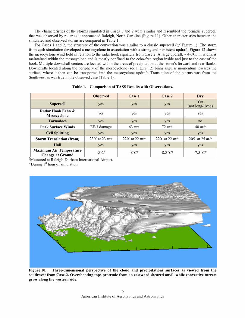
produced convective systems with different characteristics which are summarized in Tables 1 and 2. All of the environments produced strong convection, surface hail, gust fronts, strong surface winds, overshooting tops, mesocyclones, splitting updrafts, and hook echoes. A three-dimensional perspective of the simulated cumulonimbus system for Case-2 is shown in Figure 10.


9

The characteristics of the storms simulated in Cases 1 and 2 were similar and resembled the tornadic supercell that was observed by radar as it approached Raleigh, North Carolina (Figure 11). Other characteristics between the simulated and observed storms are compared in Table 1.

For Cases 1 and 2, the structure of the convection was similar to a classic supercell (cf. Figure 1). The storm from each simulation developed a mesocyclone in association with a strong and persistent updraft. Figure 12 shows the mesocyclone wind field in relation to the radar hook signature from Case 2. A large updraft, ~ 4-8km in width, is maintained within the mesocyclone and is mostly confined to the echo-free region inside and just to the east of the hook. Multiple downdraft centers are located within the areas of precipitation at the storm’s forward and rear flanks. Downdrafts located along the periphery of the mesocyclone (see Figure 12) bring angular momentum towards the surface, where it then can be transported into the mesocyclone updraft. Translation of the storms was from the Southwest as was true in the observed case (Table 1).

Table 1. Comparison of TASS Results with Observations.

Observed Case 1 Case 2 Dry

Supercell yes yes yes Yes (not long-lived)

Radar Hook Echo & Mesocyclone yes yes yes yes

Tornadoes yes yes yes no Peak Surface Winds EF-3 damage 63 m/s 72 m/s 40 m/s

Cell Splitting yes yes yes yes Storm Translation (from) 230o at 23 m/s 220o at 22 m/s 220o at 22 m/s 205o at 25 m/s

Hail yes yes yes yes Maximum Air Temperature

Change at Ground -5oC§ -8oC* -8.5 oC* -7.5 oC* §Measured at Raleigh-Durham International Airport. *During 1st hour of simulation.

Figure 10. Three-dimensional perspective of the cloud and precipitations surfaces as viewed from the southwest from Case-2. Overshooting tops protrude from an eastward sheared anvil, while convective turrets grow along the western side.


10

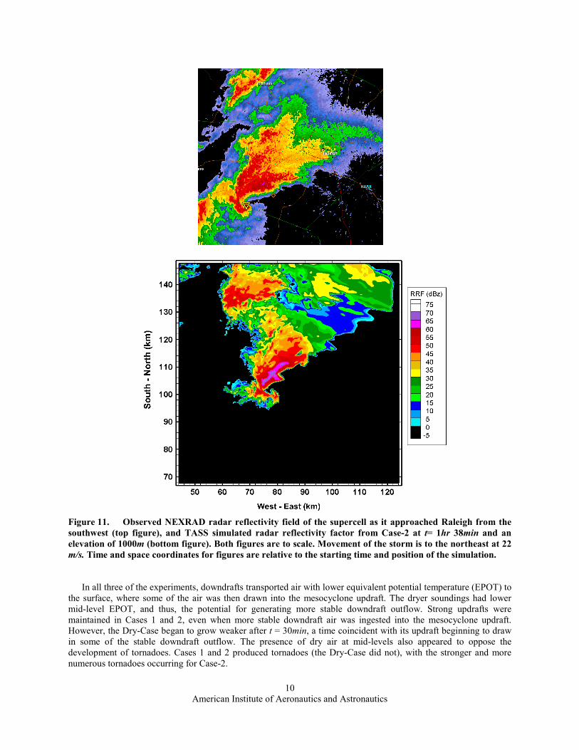
Figure 11. Observed NEXRAD radar reflectivity field of the supercell as it approached Raleigh from the southwest (top figure), and TASS simulated radar reflectivity factor from Case-2 at t= 1hr 38min and an elevation of 1000m (bottom figure). Both figures are to scale. Movement of the storm is to the northeast at 22 m/s. Time and space coordinates for figures are relative to the starting time and position of the simulation.

In all three of the experiments, downdrafts transported air with lower equivalent potential temperature (EPOT) to

the surface, where some of the air was then drawn into the mesocyclone updraft. The dryer soundings had lower mid-level EPOT, and thus, the potential for generating more stable downdraft outflow. Strong updrafts were maintained in Cases 1 and 2, even when more stable downdraft air was ingested into the mesocyclone updraft. However, the Dry-Case began to grow weaker after t = 30min, a time coincident with its updraft beginning to draw in some of the stable downdraft outflow. The presence of dry air at mid-levels also appeared to oppose the development of tornadoes. Cases 1 and 2 produced tornadoes (the Dry-Case did not), with the stronger and more numerous tornadoes occurring for Case-2.


11

Table 2. Simulated Mesocyclone Characteristics at Time of Peak Intensity.

MESOCYCLONE STRUCTURE AT 500m ALTITUDE

Case Peak

Tangential Velocity (m/s)

Diameter (km) Updraft (m/s) ΔP (mb) Time of Peak

Intensity (hr:min)

1 24 7 28 -7 1:16 2 35 5.5 30 -12 1:38

Dry 10 9 14 -3.1 0:56

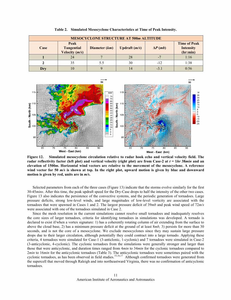
Figure 12. Simulated mesocyclone circulation relative to radar hook echo and vertical velocity field. The radar reflectivity factor (left plot) and vertical velocity (right plot) are from Case-2 at t = 1hr 38min and an elevation of 1500m. Horizontal wind vectors are relative to the movement of the mesocyclone. A reference wind vector for 50 m/s is shown at top. In the right plot, upward motion is given by blue and downward motion is given by red, units are in m/s.

Selected parameters from each of the three cases (Figure 13) indicate that the storms evolve similarly for the first

30-45mins. After this time, the peak updraft speed for the Dry-Case drops to half the intensity of the other two cases. Figure 13 also indicates the persistence of the convective systems, and the periodic generation of tornadoes. Large pressure deficits, strong low-level winds, and large magnitudes of low-level vorticity are associated with the tornadoes that were spawned in Cases 1 and 2. The largest pressure deficit of 39mb and peak wind speed of 72m/s were associated with one of the tornadoes simulated in Case 2.

Since the mesh resolution in the current simulations cannot resolve small tornadoes and inadequately resolves the core sizes of larger tornadoes, criteria for identifying tornadoes in simulations was developed. A tornado is declared to exist if/when a vortex signature: 1) has a coherently rotating column of air extending from the surface to above the cloud base, 2) has a minimum pressure deficit at the ground of at least 8mb, 3) persists for more than 30 seconds, and is not the core of a mesocyclone. We exclude mesocyclones since they may sustain large pressure drops due to their larger circulation, although potentially they could contract into a large tornado. Applying these criteria, 4 tornadoes were simulated for Case-1 (3-anticlonic, 1-cyclonic) and 7 tornadoes were simulated in Case-2 (3-anticyclonic, 4-cyclonic). The cyclonic tornadoes from the simulations were generally stronger and larger than those that were anticyclonic, and duration times ranged from 4min to 34min for the cyclonic tornadoes compared to 2min to 16min for the anticyclonic tornadoes (Table 3). The anticyclonic tornadoes were sometimes paired with the cyclonic tornadoes, as has been observed in field studies.15,16,17 Although confirmed tornadoes were generated from the supercell that moved through Raleigh and into northeastward Virginia, there was no confirmation of anticyclonic tornadoes.


12

A B

C D

Figure 13. Maximum values vs time from domains of Case-1 (red), Case-2 (blue) and Dry Case (green): A) peak vertical velocity, B) peak horizontal wind speed at an elevation of 150m, C) minimum pressure deficit at the ground, and D) maximum positive vorticity at an elevation of 150m.

Table 3. Tornadoes Generated by Cases 1 and 2 (none occurred for Dry Case).

Anticyclonic Tornadoes Cyclonic Tornadoes ID Time

(hr:min) Duration

(min) Peak

Winds (m/s)

ΔP (mb)

ID Time (hr:min)

Duration (min)

Peak Winds (m/s)

ΔP (mb)

Case-1 4-tornadoes in 120 min

1.A-1 1:04-1:20 16 n/a n/a 1.C-1 1:15-1:31 16 51 n/a 1.A-2 1:25-1:28 3 n/a n/a 1-A-3 1:52-1:53 1 45 -13

Case-2 7-tornadoes in 180 min

2.A-1 0:52-1:00 8 50 -11 2.C-1 1:39-2:13 34 72 -39 2.A-2 1:07-1:19 12 59 -14 2.C-2 2:18-2:33 15 66 -25 2.A-3 1:45-1:57 12 n/a n/a 2.C-3 2:37-2:41 4 45 n/a

2.C-4 2:58- >2 51 -13


13

Many of the simulated tornadoes were spawned within the mesocyclone, although none were generated directly from the contraction of the mesocyclone. The mesocyclone in Case-2 did intensify such that it briefly exceeded the above criteria for pressure (between t = 1hr 36.5min and 1hr 41min). At that time, the mesocyclone generated peak surface winds of 40 m/s on its northwest side and a central pressure drop of < 8mb.

Figures 14 and 15 show the tornado evolution and decay from the perspective of viewing the 8mb pressure deficit surface (this threshold is arbitrarily chosen and does not truly represent the condensation pressure surface). The evolution of the simulated tornadoes appears quite realistic as viewed from the graphical representation of the pressure deficit surfaces. Figure 14 shows the lowering of a thin funnel, its broadening as it enters into a mature phase, followed by a transition into a thin, contorted rope-like funnel just before its demise. Similar characteristics have been observed for the life stages of actual tornadoes.14 Figure 15 shows the evolution of the strongest tornado from the simulations (2.C-1) which is accompanied during part of its lifetime by an anticyclonic tornado (2.A-3). Most of the tornadoes in the simulations formed along the interface of cool air generated by the rear flanking downdrafts, and all appeared to die due to their movement into cooler downdraft outflow.

Figure 14. Three-dimensional perspective of the 8 mb pressure deficit surface as viewed from the southeast toward the rear flank of the storm. Depth of depiction is 5 km in altitude. Represented are the development and decay stages during the 15 min lifetime of the cyclonic tornado 2.C-2 (see Table 3).

Figure 15. Three-dimensional perspective of the 8 mb pressure deficit surface as viewed from the southeast toward the rear flank of the storm. Depth of depiction is 5 km in altitude. Represented is a time sequence of cyclonic tornado 2-C-1, and anticyclonic tornado 2.A-3, at t = 1:45, 1:50, 1:56, 2:07 and 2:12 (hr:min). The anticyclonic tornado forms on the left side of 2.C-1 (first sequence) and later decays leaving the cyclonic tornado in the last two sequences (see Table 3).


14

Figure 16. Cross-sections at low-altitudes through a tornado vortex pair. Plots windowed within a 9km x 9km region around the hook echo of Case-2 at t =1hr 50min. Shown are: A), radar reflectivity factor (dBZ) at 300m AGL, B), vertical velocity (m/s) at 300m AGL, C), v (northward) component of velocity (m/s) at 200m AGL, and D) equivalent potential temperature (K) at 100m AGL. The storm-relative horizontal wind vectors are included in A), B), and D). The cyclonic tornado, 2.C-1, is near the center of the subdomain, while the anticyclonic tornado, 2.A-3, is located near the bottom left corner.

The cross-sections shown in Figure 16 are at a time when the cyclonic tornado (2.C-1) was very intense and was accompanied by an anticyclonic tornado (2.A-3). The cyclonic tornado had peak surface winds of 68.5 m/s and a pressure deficit of 36.5mb (see Figure 13). About 5 mins later, the cyclonic tornado reached its maximum pressure deficit of 39mb. Figure 16 shows the position of the cyclonic tornado along the southeastern edge of the cool outflow. Its position also is within the precipitation of the radar hook signature. Some of this precipitation wraps around the tornado, with the center of the tornado embedded within radar reflectivity of 35-30dBZ. The EPOT field shows that stable downdraft air was spiraling into the tornado from the west and south sides, and warm moist air was spiraling into the tornado from the north side. It is likely that the downdraft air, although stable, supplied vorticity to be stretched in the tornado updraft. Baroclinic generation of vorticity due to temperature gradients between downdraft outflow and ambient air partly contributes to the production of vorticity as well. The surface temperature drops (not shown) were about 4oC along the edge of the outflow associated with the hook echo, and as large as 7.5oC within the outflow. The vertical motion field at 300m AGL showed general downflow within the hook appendage, which supplied outflow toward the storms rear flank. Upward motion was found along the periphery of the outflow,


15

with strong updrafts located within the tornado circulations. A strong updraft maximum also was located northwest of the cyclonic tornado and was associated with the mesocyclone circulation. The strongest upward motion shown in Figure 16B occurred within the cyclonic tornado. The vertical motion field associated with the cyclonic tornado indicated a strong annular updraft surrounding a descending core. Note that the updraft was not symmetric about the

tornado, but is strongest within the warm moist air that is spiraling into the tornado from the east. On the opposite side, relatively weaker upflow is associated with the cooler stable air that is spiraling inwards from the northwest.

A strong velocity couplet is apparent for the cyclonic as well as the anticyclonic tornado in Figure 16C. The couplet, due to its small scale, would be difficult to detect with conventional Doppler radar. However, these signatures have been detected when large tornadoes pass near a NEXRAD station,69 or when mobile research radars have been placed in close proximity of a tornado.65,70

In Figure 16, the circulation of the anticyclonic tornado is located about 4km to the west-southwest of the cyclonic tornado, and resides within the southwest edge of the outflow

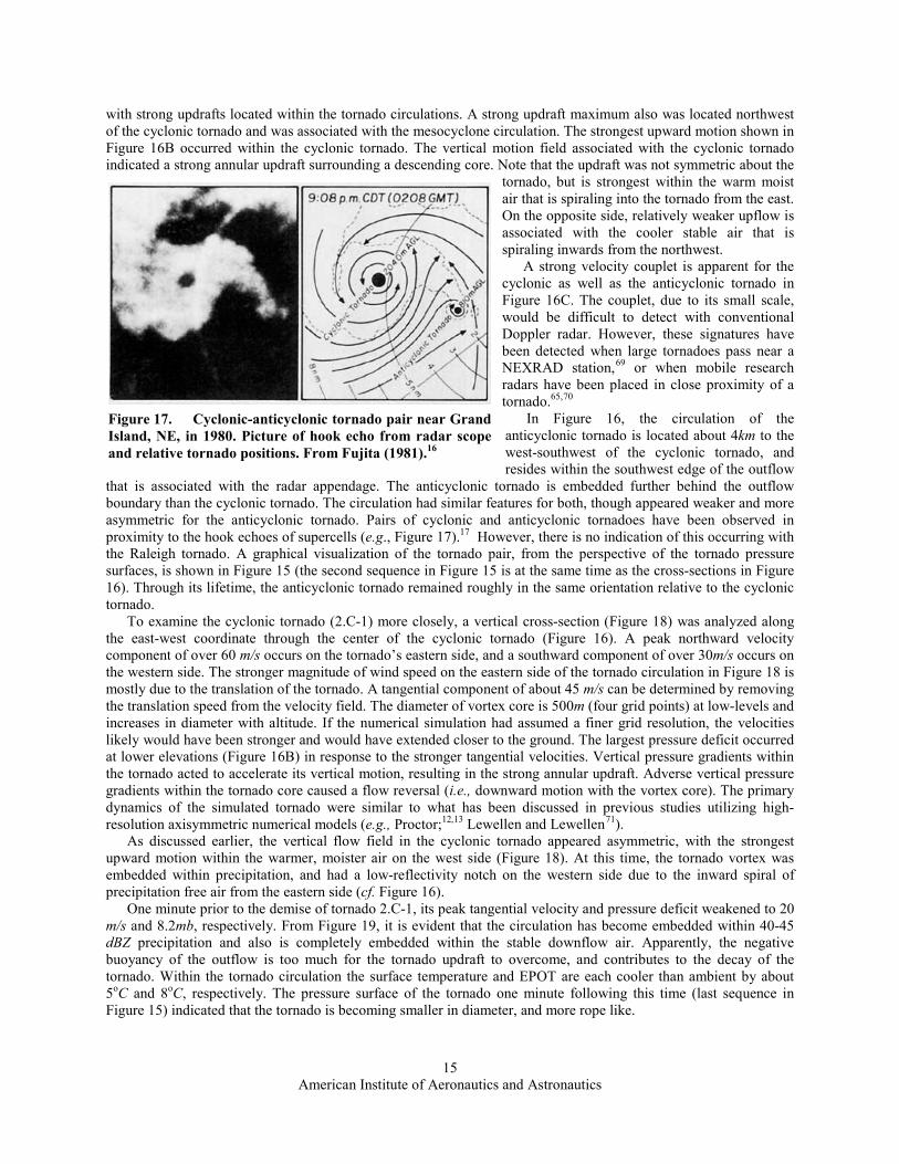
that is associated with the radar appendage. The anticyclonic tornado is embedded further behind the outflow boundary than the cyclonic tornado. The circulation had similar features for both, though appeared weaker and more asymmetric for the anticyclonic tornado. Pairs of cyclonic and anticyclonic tornadoes have been observed in proximity to the hook echoes of supercells (e.g., Figure 17).17 However, there is no indication of this occurring with the Raleigh tornado. A graphical visualization of the tornado pair, from the perspective of the tornado pressure surfaces, is shown in Figure 15 (the second sequence in Figure 15 is at the same time as the cross-sections in Figure 16). Through its lifetime, the anticyclonic tornado remained roughly in the same orientation relative to the cyclonic tornado.

To examine the cyclonic tornado (2.C-1) more closely, a vertical cross-section (Figure 18) was analyzed along the east-west coordinate through the center of the cyclonic tornado (Figure 16). A peak northward velocity component of over 60 m/s occurs on the tornado’s eastern side, and a southward component of over 30m/s occurs on the western side. The stronger magnitude of wind speed on the eastern side of the tornado circulation in Figure 18 is mostly due to the translation of the tornado. A tangential component of about 45 m/s can be determined by removing the translation speed from the velocity field. The diameter of vortex core is 500m (four grid points) at low-levels and increases in diameter with altitude. If the numerical simulation had assumed a finer grid resolution, the velocities likely would have been stronger and would have extended closer to the ground. The largest pressure deficit occurred at lower elevations (Figure 16B) in response to the stronger tangential velocities. Vertical pressure gradients within the tornado acted to accelerate its vertical motion, resulting in the strong annular updraft. Adverse vertical pressure gradients within the tornado core caused a flow reversal (i.e., downward motion with the vortex core). The primary dynamics of the simulated tornado were similar to what has been discussed in previous studies utilizing high-resolution axisymmetric numerical models (e.g., Proctor;12,13 Lewellen and Lewellen71).

As discussed earlier, the vertical flow field in the cyclonic tornado appeared asymmetric, with the strongest upward motion within the warmer, moister air on the west side (Figure 18). At this time, the tornado vortex was embedded within precipitation, and had a low-reflectivity notch on the western side due to the inward spiral of precipitation free air from the eastern side (cf. Figure 16).

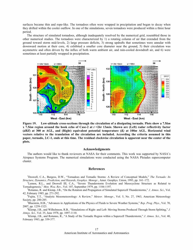
One minute prior to the demise of tornado 2.C-1, its peak tangential velocity and pressure deficit weakened to 20 m/s and 8.2mb, respectively. From Figure 19, it is evident that the circulation has become embedded within 40-45 dBZ precipitation and also is completely embedded within the stable downflow air. Apparently, the negative buoyancy of the outflow is too much for the tornado updraft to overcome, and contributes to the decay of the tornado. Within the tornado circulation the surface temperature and EPOT are each cooler than ambient by about 5oC and 8oC, respectively. The pressure surface of the tornado one minute following this time (last sequence in Figure 15) indicated that the tornado is becoming smaller in diameter, and more rope like.

Figure 17. Cyclonic-anticyclonic tornado pair near Grand Island, NE, in 1980. Picture of hook echo from radar scope and relative tornado positions. From Fujita (1981).16


16

A B

C D

Figure 18. East-West vertical cross-sections through cyclonic tornado 2.C-1 at t =1hr 50min. Shown are: A) v (northward) component of velocity (m/s), B) vertical velocity (m/s), C) radar reflectivity factor (dBZ), and D) equivalent potential temperature (K). Pressure deviation with a contour interval of 5mb overlays the w field in B), and the vortex core of the tornado is represented by the dash line in C) and D). Wind speeds in A) are ground relative. The vertical cross sections are taken at the same time as in Figure 16.

V. Summary and Conclusions A tornado-generating supercell is investigated using a large eddy simulation cloud model. The TASS model is

well suited for this application, since it has: efficient and accurate numerics, a compressible non-Boussinesq formulation for the basic governing equation set, microphysics for cloud and precipitation growth, realistic parameterization for ground stress, and subgrid closure approximations that account for the modulation of turbulence due to flow curvature.

The simulations are initialized with an environment representing the tornado outbreak that affected the Mid-Atlantic States during the Spring of 2011. The simulated supercells exhibited characteristics of classic supercells, including: 1) a large, long-lived updraft; 2) a radar hook-echo appendage; 3) a mesocyclone; 4) forward-flanking and rear-flanking downdrafts; 5) strong low-level winds; 6) heavy rainfall rates; 7) hail; 8) overshooting tops; and 9) the genesis of multiple tornadoes. The structure, scale, translation, and severity of the simulated storm resembled the actual storm that affected Raleigh, North Carolina.

The primary source of the mesocyclone’s rotation appeared to be vorticity associated with the vertical shear of the environmental winds. Storm downdrafts that were flanking the mesocyclone appeared to bring rotation from the mesocyclone to the ground. Mid-level humidity was found to be a factor in determining the occurrence and strength of tornadoes, as well as the strength of the mesocyclone. Deep moist conditions allowed rotationally-rich downdraft air to flow into the mesocyclone updraft without starving the updraft of latent energy. Both cyclonic and anticyclonic tornado families were simulated within the supercell mesocyclone. As has been found by previous researchers, the cyclonic tornadoes formed within the mesocyclone at a location near the edge of the relatively cool outflow air that was emanating from the rear flanking downdraft. In this study, tornadoes were not found to be generated by the contraction of the mesocyclone. During the decay stage of the simulated tornadoes, the pressure


17

surfaces became thin and rope-like. The tornadoes often were wrapped in precipitation and began to decay when they drifted within the cooler outflow. In one of the simulations, seven tornadoes were produced within a three hour period.

The structure of simulated tornadoes, although inadequately resolved by the numerical grid, resembled those in other numerical studies. The tornadoes were characterized by 1) a rotating column of air that extended from the ground toward storm mid-levels, 2) large pressure deficits, 3) strong updrafts that sometimes were annular with downward motion at their core, 4) exhibited a smaller core diameter near the ground, 5) their circulation was asymmetric and often driven by the influx of both warm ambient air, and rain-cooled downdraft air, and 6) were sometimes at least partially wrapped in precipitation.

Figure 19. Low-altitude cross-sections through the circulation of a dissipating tornado. Plots show a 7.5km x 7.5km region around the hook echo of Case-2 at t =2hr 13min. Shown are (Left) radar reflectivity factor (dBZ) at 300 m AGL, and (Right) equivalent potential temperature (K) at 100m AGL. Horizontal wind vectors relative to the translation of the circulation are included. According the criteria assumed in this paper, tornado, 2.C-1, ends at this time. The residual clockwise circulation is apparent near the center of the plots.

Acknowledgments The authors would like to thank reviewers at NASA for their comments. This work was supported by NASA’s

Airspace Systems Program. The numerical simulations were conducted using the NASA Pleiades supercomputer cluster.

References

1Doswell, C.A., Burgess, D.W., “Tornadoes and Tornadic Storms: A Review of Conceptual Models,” The Tornado: Its Structure, Dynamics, Prediction, and Hazards, Geophys. Monogr., Amer. Geophys. Union, 1993, pp. 161–172.

2Lemon, R.L., and Doswell III, C.A., “Severe Thunderstorm Evolution and Mesocyclone Structure as Related to Tornadogenesis,” Mon. Wea. Rev., Vol. 107, September 1979, pp. 1184-1197.

3Rotunno, R. and Klemp, J.B., “On the Rotation and Propagation of Simulated Supercell Thunderstorms,” J. Atmos. Sci., Vol. 42, February 1985, pp. 271-292.

4Fujita, T.T., “Analytic Mesometeorology: A Review,” Meteor. Monogr., Vol. 5, No. 27, 1963, American Meteorology Society, pp. 280-285.

5Bluestein, H.B., “Advances in Applications of the Physics of Fluids to Severe Weather Systems,” Rep. Prog. Phys., Vol. 70, 2007, pp. 1259-1323.

6Klemp, J.B., and Wilhelmson, R.B., “Simulations of Right- and Left- Moving Storms Produced Through Storm Splitting,” J. Atmos. Sci., Vol. 35, June 1978, pp. 1097-1110.

7Klemp, J.B., and Rotunno, R., “A Study of the Tornadic Region within a Supercell Thunderstorm,” J. Atmos. Sci., Vol. 40, February 1983, pp. 359-377.


18

8Davies-Jones, R., “Can a Descending Rain Curtain in a Supercell Instigate Tornadogenesis Barotropically?” J. Atmos. Sci.,

Vol. 65, August 2008, pp. 2469-2497. 9Markowski, P.M., Straka, J.M., and Rasmussen, E.N., “Tornadogenesis Resulting from the Transport of Circulation by a

Downdraft: Idealized Numerical Simulations,” J. Atmos. Sci., Vol. 60, 15 March 2003, pp. 795-823. 10Shabbott, C.J. and Markowski, P.M., “Surface In Situ Observations within the Outflow of Forward-Flank Downdrafts of

Supercell Thunderstorms,” Mon. Wea. Rev., Vol. 134, May 2006, pp. 1422-1441. 11Proctor, F.H., “Formation of a Tornado from a Rotating Wind Field: A Numerical Experiment,” Preprints 10th Conf. on

Severe Local Storms, American Meteorological Society, October 1977, pp. 315-321. 12Proctor, F.H., “The Dynamic and Thermal Structure of an Evolving Tornado,” Preprints 11th Conf. on Severe Local

Storms, American Meteorological Society, October 1979, pp. 283. 13Proctor, F. H., “Numerical Study on the Evolution of Tornadoes. Ph. D. Dissertation, Texas A&M University, December

1982, 267 pp. 14Golden, J.W., and Purcell, D., “Lifecycle of the Union City, Oklahoma Tornado and Comparison with Waterspouts,” Mon.

Wea. Rev., Vol. 106, January 1978, pp. 3-11. 15Brown, J.M. and Knupp, K.R., “The Iowa Cyclonic-Anticyclonic Tornado Pair and its Parent Thunderstorm,” Mon. Wea.

Rev., Vol. 108, October 1980, pp. 1626-1646. 16Fujita, T., “Tornadoes and Downbursts in the Context of Generalized Planetary Scales,” J. Atmos. Sci, Vol. 38, August

1981, pp.1511-1534. 17Fujita, T.T. and Wakimoto, R.M., “Anitcyclonic Tornadoes in 1980-1981,” Preprints, 12th Conference on Severe Storms,

American Meteorological Society, January 1982, pp. 401-404. 18Bluestein, H.B., French, M.M., Tanamachi, R.L., Frasier, S., Hardwick, K., Junyent, F., and Pazmany, A.L., “Close-Range

Observations of Tornadoes in Supercells Made with a Dual-Polarization, X-Band, Mobile Doppler Radar,” Mon. Wea. Rev., Vol. 135, April 2007, pp. 1522-1543.

19Trapp, R.J., Stumpf, G.J., and Manross, K.L., “A Reassessment of the Percentage of Tornadic Mesocyclones. Weather Forecasting, Vol. 20, February, 2005, pp. 23–34.

20Lemon, L.R., Donaldson, R.J., Burgess, D.W., and Brown, R.A., “Doppler Radar Application to Severe Thunderstorm Study and Potential Real-time Warning,” Bull. Amer. Meteor. Soc., Vol. 58, 1977, pp. 1187-1193.

21Markowski, P.M., and Richardson, Y.P., “Tornadogenesis: Our Current Understanding, Forecasting Considerations, and Questions to Guide Future Research,” Atmospheric Research, Vol. 93, 2009, pp. 3-10.

22Davies-Jones, R.P, “Streamwise Vorticity: The Origin of Updraft Rotation in Supercell Storms,” J. Atmos. Sci., Vol. 41, October 1984, pp. 2991–3006.

23Wicker, L.J., and Wilhelmson, R.B., “Simulation and Analysis of Tornado Development and Decay within a Three-Dimensional Supercell Thunderstorm,” J. Atmos. Sci., Vol. 52, August 1995, pp. 2675–2703.

24Grasso, L.D., and Cotton, W.R., “Numerical Simulation of a Tornado Vortex,” J. Atmos. Sci., Vol. 52, April 1995, pp. 1192–1203.

25McCarthy, D., and LaDune, J., “Introducing the Enhanced Fujita Scale,” National Weather Service, URL: http://www.wdtb.noaa.gov/courses/EF-scale/index.html.

26National Weather Service, URL: http://www.erh.noaa.gov/rah/news/content/20110416_raleigh_survey.pdf. 27Davies-Jones, R.P., Burgess, D., and Foster, M., “Test of Helicity as a Tornado Forecast Parameter,” Preprints, 16th Conf.

on Severe Local Storms, American Meteorological Society, 1990, pp. 588–592. 28Brooks, H.E., Doswell, C.A., III, and Cooper, J., “On the Environments of Tornadic and Nontornadic Mesocyclones,”

Weather Forecasting, Vol. 9, December 1994, pp. 606-618. 29Houze, R.A., Jr., Cloud Dynamics, Ed Academic Press, 1993, 573 pp. 30Proctor, F.H., “The Terminal Area Simulation System, Volume 1: Theoretical Formulation,” April 1987, NASA CR-4046. 31Proctor, F.H., “Numerical Simulation of Wake Vortices Measured During the Idaho Falls and Memphis Field Programs,”

14th AIAA Applied Aerodynamic Conference, Proceedings, Part II, June 1996, AIAA 96-2496, pp. 943-960. 32Proctor, F.H., “Interaction of Aircraft Wakes from Laterally Spaced Aircraft,” January 2009, AIAA 2009-0343. 33Proctor, F.H., “The Terminal Area Simulation System. Volume II: Verification Experiments,” April 1987, NASA CR-

4047. 34Proctor, F.H., “Numerical Simulations of an Isolated Microburst. Part I: Dynamics and Structure,” J. Atmos. Sci., Vol. 45,

pp. 3137-3160. 35Proctor, F. H., and Bowles, R.L., “Three-Dimensional Simulation of the Denver 11 July 1988 Microburst-Producing

Storm,” Meteorology and Atmospheric Physics, Vol. 49, 1992, pp. 107-124. 36Proctor, F.H., Hamilton, D.W., and Bowles, R.L., “Numerical Study of a Convective Turbulence Encounter,”

January 2002, AIAA 2002-0944. 37Ahmad, N.N., and Proctor, F.H., “Simulation of Benchmark Cases with the Terminal Area Simulation System (TASS),”

AIAA 2011-1005, and reprinted in Research Disclosure Journal, Database Number 564036, April 2011, 14 pp. 38Proctor, F.H., Hamilton, D.W., and Bowles, R.L., “Numerical Simulation of a Convective Turbulence Encounter,”

Preprints, 10th Conference on Aviation, Range, and Aerospace Meteorology, American Meteorological Society, May 2002, pp. 41-44.

39Ahmad, N.N., and Proctor, F.H., “Large Eddy Simulations of Severe Convection Induced Turbulence. AIAA 2011-3201.


19

40Han, J., Lin, Y.-L., Schowalter, D. G., Arya, S. P., and Proctor, F. H., "Large Eddy Simulation of Aircraft Wake Vortices

within Homogeneous Turbulence: Crow Instability," AIAA Journal, Vol. 38, February 2000, pp 292-300. 41Han, J., Lin, Y.-L., Arya, S.P., and Proctor, F.H., "Numerical Study of Wake Vortex Decay and Descent within

Homogeneous Turbulence," AIAA Journal, Vol. 38, No. 4, April 2000, pp. 643-656. 42Proctor, F.H., Hamilton, D.W., and Han, J., “Wake Vortex Transport and Decay in Ground Effect: Vortex Linking with the

Ground,” AIAA 2000-0757. 43Proctor, F.H, Hamilton, D.W., Rutishauser, D.K., and Switzer, G.F., “Meteorology and Wake Vortex Influence on

American Airlines FL-587 Accident,” April 2004, NASA TM-2004-213018. 44Proctor, F.H., Hamilton, D.W., and Switzer, G.F. “TASS Driven Algorithms for Wake Prediction,” January 2006, AIAA

2006-1073. 45Proctor, F.H., Ahmad, N.N., Switzer, G.F., and Limon Duparcmeur, F.M., “Three-Phased Wake Vortex Decay,” August

2010, AIAA 2010-7991. 46Proctor, F.H., “Three-Dimensional Simulation of the 2 August CCOPE Hailstorm with the Terminal Area Simulation

System,” Report of the International Cloud Modelling Workshop/Conference, Tech. Doc., WMO/TD – No. 139, September 1986, pp. 227-240

47Lin, Y-L., Farley, R.D., and Orville, H.D., “Bulk Parameterizations of the Snow Field in a Cloud Model,” J. Climate Appl. Meteor., Vol. 32, 1983, pp. 1065-1092.

48Proctor, F.H., “Numerical Simulations of an Isolated Microburst. Part II: Sensitivity Experiments,” J. Atmos. Sci., Vol. 46, July 1989, pp. 2143-2165.

49Rutledge, S.A., Hobbs, P.V., “The Mesoscale and Microscale Structure and Organization of Clouds and Precipitation. VII: A Model for the “Seeder-Feeder” Process in Frontal Rainbands,” J. Atmos. Sci., Vol. 40, May, 1983, pp. 1185-1206.

50Berry, E.X., and Reinhardt, R.E., “An Analysis of Cloud Drop Growth by Collection. Part I: Double Distributions,” J. Atmos. Sci., Vol. 31, October 1974, pp. 1814-1824.

51Berry, E.X., and Reinhardt, R.E., “An Analysis of Cloud Drop Growth by Collection. Part II: Single Initial Distributions,” J. Atmos. Sci., Vol. 31, October 1974, pp. 1825-1831.

52Smith, P.L., Jr., Myers, C.G., and Orville, H.D., “Radar Reflectivity Factor Calculations in Numerical Cloud Models Using Bulk Parameterizations of Precipitation,” J. Appl. Meteor, Vol. 14, 1975, pp. 1156-1165.

53Lang, S.E., Tao, W-K., Zeng, X., and Yaping, L., “Reducing the Biases in Simulated Radar Reflectivity from a Bulk Microphysics Scheme: Tropical Convective Systems,” J. Atmos. Sci., Vol. 68, October 2011, pp. 2306-2320.

54Holzapfel, F., “Adjustment of Subgrid-Scale Parameterizations to Strong Streamline Curvature,” AIAA Journal, Vol. 42, July 2004, pp. 1369-1377.

55Deardorff, J.W., “On the Magnitude of the Subgrid Scale Eddy Coefficient,” J. Comp. Phys., Vol. 7, 1971, pp. 120-133. 56Vreman, A.W., “An Eddy-Viscosity Subgrid-Scale Model for Turbulent Shear Flow: Algebraic Theory and Applications,”

Physics of Fluids, Vol. 16, October 2004, pp. 3670-3681. 57Proctor, F. H., “Numerical Simulation of Wake Vortices Measured During the Idaho Falls and Memphis Field Programs,”

AIAA 1996-2496. 58Leonard, B. P., M. K. MacVean and A. P. Lock, “The Flux-Integral Method for Multidimensional Convection and

Diffusion,” Applied Mathematical Modeling, Vol. 19, 1995, pp. 333-342. 59van Leer, B., “Towards the Ultimate Conservative Difference Scheme: V, A Second-Order Sequel to Godunov’s Method,”

Journal of Computational Physics, Vol. 32, 1979, pp. 101-136. 60Ahmad, N.N., and Proctor, F.H., “Advection of Microphysical Scalars in Terminal Area Simulation System (TASS),”

AIAA 2011-1004. 61Arakawa, A., and Lamb, V.R., “Computational Design of the Basic Dynamical Process of the UCLA General Circulation

Model,” Methods in Computational Physics, Vol. 17, 1977, pp. 173-265. 62Klemp, J. B., and Wilhelmson, R., "The Simulation of Three-Dimensional Convective Storm Dynamics," Journal of

Atmospheric Sciences, Vol. 35, June 1978, pp. 1070-1096. 63Switzer, G.F., “Validation Tests of TASS for Application to 3-D Vortex Simulations,”, October 1996, NASA CR-4756. 64Orlanski, I., "A Simple Boundary Condition for Unbounded Hyperbolic Flows," Journal of Computational Physics, Vol.

21, July 1976, pp. 251-269. 65Wurman, J., “The Multiple-Vortex Structure of a Tornado,” Weather Forecasting, Vol. 17, June 2002, pp. 473-505. 66NOAA, URL: http://rucsoundings.noaa.gov/ 67Beebe, R.G., “Tornado Proximity Soundings,” Bull. Amer. Meteor. Soc., Vol. 39, April 1958, pp. 195-201. 68Darkow, G.L., “An Analysis of Over Sixty Tornado Proximity Soundings,” Preprints, 6th Conference on Severe Local

Storms, Amer. Meteor. Soc., 1969, pp. 218-221. 69Burgess, D.W., Magsig, M.A., Wurman, J., Dowell, D.C., and Richardson, Y., “Radar Observations of the 3 May 1999

Oklahoma City Tornado,” Weather Forecasting, Vol. 17, June 2002, pp. 456-471. 70Kosiba, K. and Wurman, J., “The Three-Dimensional Axisymmetric Wind Field Structure of the Spencer, South Dakota,

1998 Tornado,” J. Atmos. Sci., Vol. 67, September 2010, pp. 3074-3082. 71Lewellen, D.C., and Lewellen, W.S., “Near-Surface Intensification of Tornado Vortices,” J. Atmos. Sci., Vol. 64, July 2007,

pp. 2176-2194.

aiaa 2012-0557 numerical simulation of a tornado generating … · 2013-04-10 · aiaa 2012-0557 ....

Documents