aiaa 2002-2985

AIAA 2002-2985Two Forms of the Rotational Solution forWave Propagation Inside Porous Channels

Joseph MajdalaniMarquette UniversityMilwaukee, WI 53233

For permission to copy or to republish, contact the American Institute of Aeronautics and Astronautics,1801 Alexander Bell Drive, Suite 500, Reston, VA, 20191-4344.

Meeting24–26 June 2002

St. Louis, MO

–1– American Institute of Aeronautics and Astronautics

Two Forms of the Rotational Solution for Wave Propagation Inside Porous Channels

Joseph Majdalani*

Marquette University, Milwaukee, WI 53233 and

Sjoerd W. Rienstra† Eindhoven University of Technology, NL-5600 MB Eindhoven, Netherlands

In this article, a long rectangular channel is considered with two transpiring walls that are a small distance apart. The channel’s head end is hermetically closed while the aft end is either open (isobaric) or acoustically closed (choked). A mean flow enters uniformly across the permeable walls, turns, and exits from the downstream end. The slightest unsteadiness in flow velocity is inevitable and occurs at random frequencies. Small pressure disturbances are thus produced. Those waves whose oscillations match the enclosure’s natural frequencies are promoted. Inception of small pressure perturbations alters the flow character and leads to a temporal field that we wish to analyze. The mean flow is of the Berman type and can be obtained from the Navier-Stokes equations over different ranges of the cross-flow Reynolds number. The unsteady component can be formulated from the linearized momentum equation. This has been carried out in numerous studies and has routinely given rise to a singular, boundary-value, double-perturbation problem in the cross-flow direction. The current study focuses on the resulting second-order differential equation that prescribes the rotational wave motion in the transverse direction. This equation exhibits unique features that define a general class of ODEs. Due to the problem’s oscillatory behavior, two general asymptotic formulations are derived, for an arbitrary mean-flow profile, using WKB and multiple-scales expansions. The fundamental asymptotic solutions reveal the same similarity parameter that controls the rotational wave character. The multiple-scales solution unravels the problem’s characteristic length scale following a unique, nonlinear variable transformation. The latter is derived rigorously from the problem’s solvability condition. The advantage of using a multiple-scales procedure lies in the ease of construction, accuracy, and added physical insight stemming from its leading-order term. For verification purposes, a specific mean-flow solution is used for which an exact solution can be derived. Comparisons between asymptotic and exact predictions are gratifying, showing an excellent agreement over a wide range of physical parameters.

I. Introduction he purpose of this paper is to obtain the fundamental asymptotic form of the rotational

solution for wave propagation inside a viscous channel bounded by transpiring walls. The original partial differential equation (PDE) stems from the momentum equation arising in the context of a fluid oscillating inside a chamber with permeable walls.1-8 Mean-flow interactions with the oscillatory motion involve

*Assistant Professor, Department of Mechanical and

Industrial Engineering. Member AIAA. †Associate Professor, Department of Mathematics and

Computing Science. Member AIAA.

unsteady inertial, convective, and diffusive mechanisms. Such interactions lead to a nonlinear scaling structure that we wish to analyze. The mean flow is of the Berman type and can be obtained from the Navier-Stokes equations over different ranges of the classical, cross-flow Reynolds number.9 Traditionally, a solution is said to be of the Berman type when it satisfies Berman’s nonlinear equation.10 The latter is a fourth-order ordinary differential equation (ODE) that arises from the two-dimensional Navier-Stokes equations applied to a porous channel, and subject to a similarity transformation. As shown in former studies,3-

7 the temporal component can be formulated from the linearized momentum equation. Accordingly, separation of variables reduces the momentum equation

T


into a coupled set of ODEs. While an exact solution can be obtained for the longitudinal set, the same cannot be said of the transverse equation. For this reason, the current study focuses on the separated, second-order differential equation that prescribes the rotational wave motion in the transverse direction. The emerging cross-flow equation defines a singular, boundary-value, double-perturbation problem exhibiting an oscillatory behavior. Such features characterize a particular class of ODEs that we wish to solve asymptotically, in general conceptual form. To set the stage, we proceed by formulating two fundamental asymptotic solutions for the cross-flow boundary-layer equation. We choose the standard WKB approach to arrive at a first-order approximation. Next, a multiple-scales procedure is implemented to produce a two-variable expansion. The latter brings into focus the emerging nonlinear scaling structure. It should be pointed out that, to the authors’ knowledge, the nonlinear coordinate transformation that is necessary for the success of the multiple-scales technique appears to be a novelty. Unlike previous studies in which the scaling transformation is conjured from guesswork or inspection, in this article, it is derived rigorously from the problem’s solvability condition. Subsequently, following the formal specification of the problem’s characteristic length scale, the multiple-scales formulation will be shown to incorporate the leading-order terms arising in the WKB approximation. Asymptotic results are verified using a special example for which the boundary-layer equation can be solved in an exact fashion. Using the exact solution as a benchmark, the truncation error is examined also. The special example that we employ stems from a practical application. In fact, both exact and asymptotic formulations serve as useful extensions to a recent study that considers the oscillatory flow inside rectangular cavities.1-3 Such flows take place in a number of interesting applications, including cold-flow simulations of burning propellant,5-8 isotope separation,9-11 turbulence of oscillatory flows,12-17 filtration mechanisms,18 and sweat cooling.19

II. Physical Setting Our interest lies in an ideal gas performing small oscillations (at an angular frequency ω ) about a steady two-dimensional velocity field. The solution domain consists of a long and narrow rectangular channel of length ,L height 2h , and width w . The channel is closed at the head end and either a) choked or b) open (isobaric) at the downstream end (see Fig. 1). Furthermore, we select a Cartesian reference frame that is anchored at the head-end centre, and use x and y to

represent the cross-flow (normal) and streamwise (longitudinal) coordinates (normalized by h ). For the reader’s convenience, the complete details that may be found in other work2,3 are briefly revisited in this section. For periodic pressure perturbations of amplitude P , one can express the total velocity profile as a sum of its mean and time-dependent components:

[ ]1 1 ˆ( , , ) ( , ) ( , , ) ( , , )x y t V x y P a x y t x y tρ − −= + +u u u u , (1) where V is the gas velocity at the transpiring wall, ρ is the gas density, a is the acoustic speed of sound, and t is dimensional time. In (1), the normalized mean velocity is ( , )u=u v while ˆ ˆ ˆ( , )u=u v and ( , )u=u v denote the irrotational (curl-free) and solenoidal (divergence-free) time-dependent components.3 The oscillatory pressure ( , )p y t is of the form cos( ) exp( )p P ky i tω= − , (2) and the corresponding irrotational velocity response in a rectangular cavity will be:2,3 [ ]ˆ 0, sin( ) exp( )i ky i tω= −u . (3) Here k is the dimensionless wave number, and ω is the dimensional frequency corresponding to an oscillation mode number 1, 2,3, ,m = ∞… . The patterns associated with the mode numbers are known as the fundamental, first harmonic, second harmonic, etc., oscillation mode shapes. In practice, the lowest oscillation mode shapes require the least energy to excite and are therefore the most likely to occur. Depending on whether the downstream end is a) closed (acoustically non-compliant) or b) open (isobaric), the wave number and frequency of oscillations are given by:1

/ ( )( ½) / ( )m h L a

km h L bπ

π

= −,

/ ( )( ½) / ( )m a L am a L bπ

ωπ

= −

. (4)

The rotational velocity component can be derived from the linearized momentum equation known to the order of the cross-flow Mach number /M V a= . In fact, one may follow Majdalani,3 Flandro,4-6 or Majdalani and Van Moorhem,7 and express the momentum equation in the streamwise direction. The result is

( )2

2 2 0V ut h x y h x

ν ∂ ∂ ∂ ∂+ + − = ∂ ∂ ∂ ∂

v v vvv ; (5)

where ν is the kinematic viscosity. For equal permeability at the walls, symmetry enables us to reduce the domain to 0 1x≤ ≤ and 0 /y L h≤ ≤ . This self-imposed condition prevents our model from accommodating asymmetrical mean-flow solutions. In the case of transpiring walls, however, only unique and stable symmetrical solutions exist for the entire range of the injection Reynolds number defined by Eq. (7). This conclusion was first drawn by Skalak and Wang20 and later proved rigorously by Shih.21 For suction flows


with 6.0014R < − , multiple solutions can exist including those exhibiting asymmetrical behavior. For a thorough investigation of all possible solution patterns that accompany flow withdrawal, the reader is referred to the comprehensive work by Zaturska, Drazin and Banks.22 For two-dimensional and three-dimensional considerations, the reader may also find interesting the studies by Cox23 and Taylor, Banks, Zaturska and Drazin.24 In addition to the geometric symmetry that is imposed, the no-slip condition at the wall requires that ˆ 0+ =v v . Thus, one must have,

(1, , ) sin( ) exp( )y t i ky i tω= − −v , (0, , ) / 0y t x∂ ∂ =v . (6) Setting exp( )i tω= −v v in (5) gives

( )2

21 0iS u

x y R x∂ ∂ ∂

− + + − =∂ ∂ ∂v vv vv ; (1, ) sin( )y i ky= −v ,

(0, ) / 0y x∂ ∂ =v , hSVω

≡ , VhRν

≡ . (7)

Here S and R are the Strouhal and cross-flow Reynolds numbers, respectively. The reciprocal of R , namely, 1Rε −≡ , is taken, henceforward, to be the primary perturbation parameter. Due to practical limitations on viscosity and frequency, meaningful physical settings correspond to 10R > (cf. Yuan11). Furthermore, for nontrivial injection, the convection speed at the transpiring walls must exceed the molecular diffusion speed ων . Since 2/ /S R Vων= ,

imposing V ων≥ requires that S R≤ . The possible equality (V ων= , S R= ) corresponds to the case for which the walls behave as if they were impermeable. In that limiting process of insignificant injection, one can choose (for both physical and perturbation reasons)

10S R= = to set the lower bounds of the physical domain. This limit is partly inspired by the fact that a value of 10S < is uncommon in oscillatory systems. Practical applications will hence correspond to

10R S> > . The value of R (here positive for influx) has been the basis for mean-flow velocity assessments that have received considerable attention in the past. In fact, one may enumerate a great number of studies concerned with the mean-flow structure, uniqueness, and stability.9-11,20-31 Presuming a separable solution of the form

( , ) ( ) ( )x y f x g y=v and using the known profile ( , )x y= −u for flow inside a cavity,32 (7) becomes

( )2

21 1 n

f x f y giSRf x f x g y

λ+ + − = =d d dd d d

, (8)

where nλ must be strictly positive for a nontrivial formulation. Linear summation over nλ gives

( ), ( ) nn n

n

x y c f x yλ

λ= ∑v . (9)

Tacitly it is assumed that the collection of nf functions forms a complete basis in some functional space, especially in neutrally stable or unstable mean

z

yx

0

1

0

1

2 4 6 8y

x

Fig. 1 Sketch of two-dimensional geometry and solution domain.


flows. A similar example includes the representation of trailing vorticity in the critical layer of a highly viscous boundary layer. Furthermore, satisfaction of the boundary conditions in (7) yields 2 1( 1) /(2 1)!n n

nc i k n+= − − + , 2 1,n nλ = + 0,1,n = … , (1) 1nf = , and (0) 0nf ′ = . The separated

solution nf is left to be determined from the cross-flow boundary-layer equation nf

( )[ ]2 2 0n n nf xf n iS fε ′′ ′+ + − + + = . (10) Once nf is known, the rotational component of the velocity can be constructed via (9). One obtains

2 1

0exp( ) ( 1) ( ) ( ) /(2 1)!n n

nn

i i t ky f x nω∞

+

=

= − − − +∑v (11)

Fortuitously, the cross-flow boundary-layer equation (10) can be solved both exactly and asymptotically. However, for more sophisticated mean-flow profiles that are solutions to Berman’s equation,10 the resulting boundary-layer equations can be solved asymptotically only. In what follows, two fundamental asymptotic solutions are constructed for the class of ODEs to which (10) belongs.

III. Fundamental Formulation When coupling exists inside an enclosure between a mean-flow structure and small-amplitude pressure perturbations, the linearized momentum equation has been shown in several studies to be reducible by separation of variables (cf. Flandro,4-6 Majdalani and Van Moorhem,7 and Majdalani33). As outlined in the previous section, former studies have demonstrated that a successful outcome relies on resolving the separated cross-flow boundary-layer equation. The latter contains two perturbation parameters and exhibits the fundamental form

[ ]2

2d d( ) ( ) ( ) 0d d

f fa x b x i c x fx x

ε λ+ + + = ; ( ) 0a α = ; (12)

where x is defined over a closed interval, xα β≤ ≤ ; ( )a x , ( )b x and ( )c x are real coefficients; 1i = − ; and

ε is the primary perturbation parameter associated with small viscosity. For influx at the walls, ( ) 0a x > . The Strouhal number is represented by the secondary perturbation parameter λ , which is a measure of unsteadiness. Typically, 10R λ> > for nontrivial oscillations and flow influx. Because of symmetry about the core, ( ) 0a α = fulfils the physical need for a vanishing transverse component of the velocity.10 Boundary conditions accompanying (12) consist of

d ( ) 0df

xα

= , ( )f β γ= . (13)

A. Motivation As illustrated in (10), ( ) 0a α = gives rise to a regular singularity. This singularity is of a logarithmic type that demands a careful application of perturbation tools. Since an exact solution is always desirable, the forthcoming conceptual solution will be later compared to the exact solution of (10). When the undisturbed state is taken to correspond to more elaborate mean-flow solutions of the Berman equation,10 more complicated expressions for ( )a x , ( )b x and ( )c x will arise. The fundamental asymptotic formulations that will be developed below can then be used to obtain closed-form temporal solutions for specific mean-flow patterns. The conceptual solutions can also reveal the characteristic length scales and dynamic parameters that control the rotational wave behavior (amplitude, phase, and depth of penetration) for an arbitrary mean-flow profile.

B. Fundamental WKB Solution Consider the singular, boundary-value, double-perturbation problem expressed by (12)-(13). Conventional WKB theory (cf. Bender and Orszag34) proposes setting

( )1 2 30 1 2 3 4( ) expf x S S S S Sγ δ δ δ δ−= + + + + +… ; (14)

where δ is a small parameter and ( )jS x ( 0j ≥ ) must be determined in succession. Following substitution into (12) and normalization, the distinguished limit for

1λ ε −< is found to be δ ε= . Collecting terms of the same order in ε produces the defining equations. Provided that ½~λ ε − , the zeroth-order equation for 0S at ½( )ε −O is ½

0 0a S i cε λ− ′ + = . Therefore,

10 d

xS i a c t

βλ ε −= − ∫ . (15)

Similarly, the companion equation at (1)O can be written as 2

1 0 0aS S b′ ′+ + = . Hence,

( ) ( )1 2 1 2 2 21 0 d d

x xS a b S t a b c a t

β βελ− − −′= − + = − −∫ ∫ . (16)

Next, the ( )εO equation can be obtained via 2 0 0 12 0aS S S S′ ′′ ′ ′+ + = . The result is

( )12 0 0 12 d

xS a S S S t

β− ′′ ′ ′= − +∫

( ) 3 2 3 52 2 dx

i ac ca bc a c a tβ

λ ε ελ− − ′ ′= − − + ∫ (17)

Higher-order terms can be found from 3 1′ ′′+aS S 2

1 0 22′ ′ ′+ +S S S 0= , and 4 2 0 3 1 22 2 0aS S S S S S′ ′′ ′ ′ ′ ′+ + + = . One finds

( ) ( )2 3 2 2 2 53 6 5 4

xS ab ba b a c b c a acc a

βελ− − ′ ′ ′ ′= − − + + −∫

2 4 4 75 dc a tε λ − − , (18)


( 24 4 10 4 6

xS i acb bca abc b c

βλ ε ′ ′ ′= − + −∫

)2 2 5 2 4 5 93 3 14a c ca caa aa c a c aε λ− −′′ ′ ′′ ′ ′− − + + −

( )2 3 2 3 722 16 20 dc a ac c bc a tελ − ′ ′+ − + . (19)

The same can be applied to any desired order. For example, one can write

( )1 25 3 0 4 1 3 22 2 d

xS a S S S S S S t

β− ′′ ′ ′ ′ ′ ′= − + + +∫ , (20)

( )16 4 0 5 1 4 2 32 2 2 d

xS a S S S S S S S t

β− ′′ ′ ′ ′ ′ ′ ′= − + + +∫ , (21)

( )1 27 5 0 6 1 5 2 4 32 2 2 d

xS a S S S S S S S S t

β− ′′ ′ ′ ′ ′ ′ ′ ′= − + + + +∫ , (22)

( )18 6 0 7 1 6 2 5 3 42 2 2 2 d

xS a S S S S S S S S S t

β− ′′ ′ ′ ′ ′ ′ ′ ′ ′= − + + + +∫ (23)

In general, two recurrence formulae based on 0S and 1S can yield jS , 2j∀ ≥ ; these formulae can be defined

for 0,1,r = … such that

12 2 2 2 1

02 d

rxr r k r k

kS a S S S t

β−

+ + −=

′′ ′ ′= − +

∑∫ , (24)

1 22 3 2 1 2 2 1

02 d

rxr r k r k r

kS a S S S S t

β−

+ + + − +=

′′ ′ ′ ′= − + +

∑∫ . (25)

Since δ ε= , 0S , 1S and 2S are required to determine the solution at ( )εO . Two additional corrective terms will be needed to arrive, each time, at the next integral order in ε . For example, letting

1( ) ( ) dx

w x b i c a tλ −≡ − +∫ , the leading-order WKB solution can be expressed as

(0) ( )f x

122 2 3

2exp ( ) ( ) d ( )x

w x w c a t Sβ

γ β ελ ε ε− = − + + + ∫ O

( {2 2 3 1exp ( ) ( ) +x

w x w c a iβ

γ β ελ λ− −= − + ∫

( ) } )3 2 3 5 2 2 d ( )ac ca bc a c a tελ ε− − ′ ′× − − + + O (26)

The basic solution indicates that results can be expressed, everywhere, as function of λ and the viscous parameter 2ξ ελ≡ . In like fashion, higher-order expressions can be represented by

[(1) ( ) exp ( ) ( )f x w x wγ β= − 2 2 3dxc a t

βελ −+ ∫

31

2 2 22 3 4 ( )S S Sε ε ε ε+ + + +

O (27)

[(2) ( ) exp ( ) ( )f x w x wγ β= − 2ελ+ 2 3dxc a t

β−∫

3 51

2 2 22 32 3 4 5 6 ( )S S S S Sε ε ε ε ε ε+ + + + + +

O , (28)

so that, j∀ , the solution can be written as 2

( ) 2 2 3 12

0exp ( ) ( ) d

βγ β ελ δ− +

+=

= − + +

∑∫

jxj rr

rf w x w c a t S

1( )jε ++O . (29) Splitting the summation into even and odd powers of δ , one obtains

(( ) 2 2 3( ) exp ( ) ( ) dxjf x w x w c a t

βγ β ελ −= − + ∫

1

2 1 2 2 12 2 2 3

0 0( )

j jr r j

r rr r

S Sδ δ ε−

+ + ++ +

= =

+ + +

∑ ∑ O (30)

The recurrence formulae given by (24)-(25) can now be substituted into (30). One finds

{( ) ( ) exp ( ) ( )jf x w x wγ β= −

122 2 3 1

2 2 10 0

2j rx r

r k r kr k

c a a S S Sβ

ελ ε +− −+ −

= =

′′ ′ ′+ − +

∑ ∑∫

11 1 2

2 1 2 2 10 0

2 dj r

rr k r k r

r ka S S S S tε

−+ −

+ + − += =

′′ ′ ′ ′− + +

∑ ∑ 1( )jε ++O

(31) The above generalization enables us to determine the WKB solution to any desired order j . In the forthcoming analysis, we shall define our basic WKB solution to be W (0) ( )f f ε= +O . In order to determine the model’s characteristic length scale and for the purpose of gaining a better understanding of the inner scaling constitution, the method of multiple scales will be employed next.

C. Two-variable Multiple-scales Expansion A two-variable multiple-scales procedure requires specifying two fictitious coordinates, an outer scale 0x , which is routinely taken to be the unmodified independent variable, and an inner scale, 1x , that can capture rapidly changing behavior. Traditional inner scale choices include linear transformations of the form 1 ( )x xδ ε= or 1 / mx x ε= , (32) where the function ( )δ ε or the stretching exponent m are determined from foreknowledge, rationalization, order-of-magnitude scaling, or plain guessing. We find such linear transformations to be unproductive in the case at hand. In fact, we find it far more expedient to introduce a nonlinear variable transformation of the form,


1 ( )x s xε= , (33) where ( )s x is a scale function that can accommodate nonlinear scaling assortments. This choice provides the necessary freedom to achieve a balance in the governing ODE between diffusive, convective, and inertial terms. A similar choice of a nonlinear transformation was determined to be necessary and thus employed recently by Zhao et al.,35 Staab and Kassoy,36 Majdalani,33 and Majdalani and Van Moorhem.7 The current study will obviate the need for conjecture because the correct nonlinear scaling transformation will be derived directly from the problem’s solvability condition. As one would expect, the corresponding results will be more accurate, uniform, and widely applicable than those obtained from the use of other scalings. In the generalized two-variable scheme, we choose

0x x= to be the base, and 1 0( )x s xε= to be the modified coordinate. Substitution into (12) yields

( )2

220 0 1

( ) 0f f fa a s b i c fx x x

ε ε λ ε∂ ∂ ∂′+ + + + + =∂ ∂ ∂

O , (34)

where primes denote differentiation with respect to x . Next, we consider a Poincaré expansion of the form

M (0) (1) 2( )f f fε ε= + +O , where (0)f is the leading-order term that we propose to find, and Mf is the asymptotic formulation based on multiple scales. Inserting the two-term expansion of Mf into (34) gives

( )(0)

(0)

0

fa b i c fx

λ ∂

+ + ∂ ( )

(1)(1)

0

fa b i c fx

ε λ ∂

+ + + ∂

(0) 2 (0)

21 0

f fasx x

∂ ∂′+ + ∂ ∂ 2( ) 0ε+ ≡O . (35)

where (1)λ =O is fixed. Quantities between brackets must vanish independently, ε∀ . Following standard multiple-scales arguments, the leading-order equation, namely,

( )(0)

(0)

0

0fa b i c fx

λ∂+ + =

∂ (36)

gives

(0)0 1( , )f x x = 0( )

1 1( ) w xC x e

0 10( ) ( ) d

xw x b i c a tλ −≡ − +∫ (37)

At the outset, the first-order equation in ε becomes

( )(1) (0) 2 (0)

(1)2

0 1 0

f f fa b i c f asx x x

λ∂ ∂ ∂′+ + = − −∂ ∂ ∂

(38)

The procedure needed to arrive at a uniformly valid (1)f can be used to provide the additional information

necessary to specify 1C . However, in order to

determine 1C , it is not necessary to determine (1)f fully. It is sufficient to formulate a solvability condition for which a solution for (38) exists in a manner to ensure an asymptotic series expansion of the form

(0) (1) ( )f f oε ε+ + . Evidently, the goal is to find a solution (1)f that does not grow such that (1)fε and

(0)f become comparable. For this, it is convenient to introduce the ratio

(1)

0 10 (0)

0 1

( , )( )( , )

f x xh xf x x

= (39)

In order to determine h , it is expedient to first multiply (36) by 1 (1) (0) 2[ ]a f f− − and subtract the outcome from (38) multiplied by (0) 1[ ]af − . Forthwith, terms containing ( )b i cλ+ cancel out. One is left with

(1) (1) (0)

(0) (0) 20 0

1[ ]

f f ff x f x

∂ ∂−

∂ ∂

(0) 2 (0)

(0) (0) 21 0

1s f ff x af x

′ ∂ ∂= − −

∂ ∂ (40)

Grouping the left-hand-side and using (39), (40) can be simplified into

(0) 2 (0)

(0) (0) 20 1 0

1h s f fx f x af x

′∂ ∂ ∂= − −

∂ ∂ ∂ (41)

D. Solvability Condition In order to ensure a valid asymptotic series expansion, the ratio of (1)f and (0)f must be bounded. This can be accomplished by imposing the following solvability condition:

0(1) (0) 2 (0)

(0) (0) (0) 21 0

1 d (1)xf s f fh t

f f x af x ′ ∂ ∂

= = − + = ∂ ∂ ∫ O ,

1x∀ , 10 ( )x ε −=O . (42)

Since (0)f = 0( )1 1( ) w xC x e , (42) becomes

02

1 1

1 1 1

( ) d ( ) ( ) ( ) d( ) d ( )

x s t C x w t w th tC x x a t

′ ′′ ′+= − +

∫ .

02

0 1 1

1 1 1

( ) d ( ) ( ) ( ) d (1)( ) d ( )

xs x C x w t w t tC x x a t

′′ ′+= − − =

∫ O (43)

For general a , b , and c , (43) can only be true ( 1x∀ , 1

0 ( )x ε −=O ) if, and only if

1 1

1 1 1

1 d ( )( ) d

C x KC x x

= = constant 1 1 0 1( ) exp( )C x C K x⇒ =

(44) Here, 0C is a pure constant to be evaluated from (13). On the other hand, K is a subsidiary constant brought about by the introduction of the scale functional ( )s x . When (44) is substituted back into (43), ( )s x can be


obtained in a manner to ensure that h remains bounded. This yields, in general

02

1 10 0

( ) ( )( ) ( ) d( )

x w t w ts x K h x K ta t

− − ′′ ′+= − −

∫ , (45)

where ( )h x can be any bounded function. The freedom in selecting ( )s x enables us to satisfy (45).

E. A Two-variable Multiple-scales Solution After returning to the original variable x , (45) can be inserted back into (44) and (37). As K cancels out, the leading-order solution becomes

( )(0) 2 10 exp ( ) d ( )

xf C w x w w a t h xε ε− ′′ ′= − + − ∫

( )2 10 exp d ( )

xC w w w a tε ε− ′′ ′= − + + ∫ O . (46)

This is due to ( ) (1)h x =O and, thereby, exp( ) 1 ( )hε ε− = +O . It transpires that h plays no role and, therefore, can be omitted at ( )εO . After specifying

0C from (13), the complete solution can be combined into

{ }M 2 1( ) exp ( ) ( ) ( ) ( ) ( ) dx

f x w x w w t w t a t tβ

γ β ε − ′′ ′= − − + ∫ ( )ε+O , (47)

where 22 2 2 2[( ) ( 2 )]w w c b a b ab i a c ac bc aλ λ −′′ ′ ′ ′ ′ ′+ = − + + − + − +

(48) The leading-order multiple-scales solution is, therefore,

( )( )

2 3 2 2 3M2

1 3

( ) ( )

expdt

2

x

w x w

c a ab a b b af

i ac ca bc aβ

β

λγελ

λ

− − −

− −

− ′ ′+ − −= + ′ ′+ − −

∫

(49) It should be noted that, for the specific boundary value problem at hand, Mf contains a higher-order correction of order ( )εO . This is apparent in the second term of the integrand, in ( )2 2 2 3d

xab a b b a t

βελ λ− −′ ′− −∫ .

Although this correction can lead, in general, to a higher-order approximation, it must be suppressed for consistency in the perturbative sequence. The uniformly valid leading-order solution becomes

{M ( ) exp ( ) ( )f x w x wγ β= −

( ) }2 2 3 1 32 d ( )x

c a i ac ca bc a tβ

ελ λ ε− − − ′ ′+ + − − + ∫ O (50)

By comparison with Wf in (26), Mf shares the same dominant arguments. However, the imaginary part of the integrand in (50) does not contain the secondary correction, 2 3 3 52 d

xi c a t

βε λ −∫ , that is present in Wf .

This leads to a simpler expression that is more likely to be integrated into a closed form given some arbitrary coefficients c and a . Here again, the parameter

2ελ

appears to be in control of exponential damping (and hence, of penetration depth) of the rotational wave function. Since 2w w′′ ′+ is dominated by 2 2 2c aλ −− , it is clear from (45) that

2 3( ) dx

s x c a t−∫∼ (51)

IV. Specific Example Consider the example described in Section 2 and leading to (10). The corresponding problem is characterized by a x= , (2 2), 0,1,b n n= − + = … , 1c = ,

1Rε −= , Sλ = , 0α = , 1β = , and 1γ = . We propose to solve this equation both exactly and asymptotically. We also propose to examine its inherently nonlinear scaling composition using both standard methods and the newly obtained expressions.

A. Exact Solution It is expeditious to apply on (10) a Liouville-Green transformation of the form

X x R= , 214exp( ) ( )= −nf X F X , 3 2p n iS= − − + (52)

This eliminates the first derivative and converts (10) and its boundary conditions into

21 12 42 ( ) 0F p X F

X+ + − =

2dd

,

14( ) exp( )F R R= , (0) 0F

X=

dd

. (53)

Equation (53) has a standard solution that can be written in terms of the parabolic cylinder function

( )pD X , namely,

1 2( ) ( ) ( )p pF X C D X C D X= + − . (54) It is instructive to note that, since Re( ) 0p < , one can use (formula 9.241.2 in Gradshtein and Ryzhik37):

1 2 1 21 14 20

( ) [ ( )] exp( ) exp( )ppD X p X Xτ τ τ τ

∞− − −= Γ − − − −∫ d

(55) where Γ is Euler’s Integral of the second kind. Careful application of boundary conditions renders, after some effort,

12 (1 ) 1

1 22(0) 2 [ (1 )]( ) / ( ) 0pF p C C p− +′ = − Γ − − Γ − = (56)

/ 2 1 1 1 1 11 2 2 2 2 2 22 exp( ) ( ) /[ ( ) ( , , )]pC C R p p p R= = Γ − Γ − Φ −

(57) where Φ is Kummer’s confluent hypergeometric function given by


2( 1)( , ; ) 1

1! ( 1) 2!+

Φ = + + ++

…a x a a xa b xb b b

(58)

Finally, using the superscript E for ‘exact,’ one obtains E 2 21

2( ) exp[ ( 1)]nf x Rx x−= −

2 11 1 1 1 1 12 2 2 2 2 2 ( , , ) ( , , )p Rx p R−× Φ − Φ − (59)

By simple rearrangement, the exact solution can be used to reveal the action variables in the problem:

E 1 2 212( ) exp[ ( )( 1)]nf x x xε − −= −

1 2 1 11 1 1 1 1 12 2 2 2 2 2 ( , , ) ( , , )p x pε ε− − −× Φ − Φ − . (60)

Clearly, the 2/ xε scale appears explicitly in (60).

B. WKB Solution In seeking an asymptotic solution for (10), it should be noted that two cases must be considered depending on the order of the secondary perturbation parameter. These two cases correspond to (1)S =O and

( )S R=O .

1. Failure of the Traditional Outer Expansion For (1)S =O , (1)x =O , one must derive, at leading order, the outer solution o

nf from

( )[ ]2 2 0o on nxf iS n f′ + − + = , (1) 1o

nf = ,

or 2 2( ) exp( ln )o nnf x x iS x+= − . (61)

On the one hand, the 2 2nx + factor in onf decays

rapidly as 0x → . As a result, the remaining boundary condition at the origin is automatically satisfied by the first derivative. This obviates the need for an inner solution at this order. On the other hand, the exponential term in o

nf represents an oscillatory behavior that is rapid for large S . Since S can be large in practice, the rapid oscillations that occur on a shorter scale preclude the possibility of a uniformly-valid solution. This can be seen in the expression for the first-order correction when the outer solution is written at

2( )εO :

2 2( ) exp( ln )o nnf x x iS x+= − { 21 2 (2 1)S n nε + − + +

] }2 2(4 1) ( 1) / 2 ( )i n S x ε−− + − +O . (62) In fact, since the correction term comprises a part of

2( )SεO , nonuniformity can be expected at large S . A regular perturbation solution is hence expected to fail when S R∼ .

2. The WKB Expansion for ( )S R=O

Using (26), the leading-order WKB solution can be written as

((0) 2 2 212exp ( 1)n

nf x xξ+ −= − − {lniS x−

}2 2 212 ( 1) 3 4 ( 1) ( )S x n xξ ξ ε− − − + − + + + + O (63)

It is reassuring that both (0)nf and o

nf reduce to the same expression in the limit as 0ξ → and (1)S =O . Since 2Sε ξ −= , fixing S requires that 0ε → whenever 0ξ → . The outcome is

(0) 2 2

0 0const const

exp( ln )lim lim o nn n

S S

f f x iS xξ ε

+

→ →= =

= = − . (64)

One may also obtain, after some effort, the first and second-order WKB solutions from (27) and (28). These are

((1) 2 2 212exp ( 1)n

nf x xξ+ −= − − { 2 21 2(1 3 2 )S n n− − + +

}2 2 4 2512 3(7 12 )( 1) ( 1)n x x xξ ξ− − − + + + + + +

(2 2 212ln ( 1) 3 4 ( 1)iS x S x n xξ ξ− − −− + − + + +

{2 2 216 ( 1) 3(7 28 24 )S x n nξ − −− + + + 4 (9 20 )nξ+ +

}) )2 2 1 2 4 2( 1) 21 ( 1) ( )x x xξ ε− − − − × + + + + + O (65)

( {(2) 2 2 2 212exp ( 1) 1n

nf x x Sξ+ − −= − − + 22(1 3 2 )n n− + +

2 2 4 2512 3(7 12 )( 1) ( 1)n x x xξ ξ− − −− + + − + +

{2 2 2 3( 1) (1 7 14 8 )S x n n nξ − −+ + + + +

2 2 2 1 22 13 4(10 54 60 ) ( 1) (47 140 )n n x x nξ ξ− − − + + + + + + +

} }4 3 6 2 2 1425 ( 1) ( 1)x x x x iSξ− − − − − × + + + + + −

(2 2 2 2 212ln ( 1) 3 4 ( 1) ( 1)x S x n x S xξ ξ ξ− − − − −× + − + + + + +

{ 212 (7 28 24 )n n× − + + [ 21

3 2(9 20 ) n Sξ −− + −

2 3 2 2 1 212 (9 80 216 160 ) ( 1)n n n x x ξ− − − × + + + + + −

2 2 4 3 225 7 (25 188 280 ) ( 1)S n n x Sξ− − − × − + + + +

6 2 2 1 4 2 (59 252 ) ( 1) 22n x x x Sξ− − − − − × + + + + +

}) )8 4 3( 1) ( )x x ε− − × + + + O (66)

3. Endpoint Singularity at Even Orders of ε It should be noted that, as 0x +→ , the WKB solution at even orders of ε becomes suddenly unbounded. For example, regardless of S or n , the real part of the exponential argument in (1)

nf is dominated at the origin


by ( )2 2 2 4 3 2 65 512 3 6 0

( 1) 1 ~ .ξ ξ ξ +− − − − −

→− − − → +∞

xx S x S x

Since the wave amplitude is prescribed at the origin by ( )2 2 3 2 65

6expnx S xξ+ − − , the exponential singularity at 0x = cannot be overcome by the vanishing polynomial

to any given power of 2 2n + . Interestingly, this unbounded character alternates between successive orders. In fact, it can be shown that, in the limit as

0x +→ , the WKB solutions at progressive orders are dominated by

( )(0) 2 2 212expn

nf x xξ+ −−∼ ,

( )(1) 2 2 3 2 656expn

nf x S xξ+ − −+∼ ,

( )(2) 2 2 5 4 10215expn

nf x S xξ+ − −−∼ (67)

so that, at any order j , one has

1 2 1 22 1( ) 2 2

2(2 1)

( 1)exp

2(2 1)ξ+ + −

+++

−

+ ∼

j j jjj n

n j

M Sf xj x

; 0x +→ (68)

The leading-order asymptotic coefficients are

0 1 1M M= = , 2 2M = , 3 5M = ,

4 14M = , 5 42M = , 6 132M = , 7 429M = , … (69) These numbers form a progression whose first eleven odd coefficients are

{1,5, 42, 429, 4862,58786,742900,9694845

},129644790,1767 263190, 24 466 267 020 (70) After some effort, one realizes that this progressive sequence can be generated from the recurrence formula

0 1M ≡ , 1

22 1 2

02

j

j k j k jk

M M M M−

+ −=

= +∑ , 0j ≥ (71)

where the even numbers must be derived from

1

2 2 10

2j

j k j kk

M M M−

− −=

= ∑ , 1j ≥ . (72)

For example, in order to find the asymptotic form of (3)

nf near the origin, 7M must be evaluated from

2

27 6 3

02 k k

kM M M M−

=

= +∑

20 6 1 5 2 4 32( ) 429M M M M M M M= + + + = (73)

where2

6 5 0 5 1 4 2 30

2 2( ) 132k kk

M M M M M M M M M−=

= = + + =∑

The near-core behavior of the solution becomes

( )(3) 2 2 7 6 1442914 0 , , ,

expnn x n S

f x S xξ

ξ ++ − −

→ ∀→ +∞∼ . (74)

Inasmuch as the singularity at 0x +→ causes the solution to become nonuniformly valid, the reader is

cautioned that ( )jnf is secular-free for even values of j .

The use of (1)nf , (3)

nf , etc., leads to an incomplete representation that lacks small boundary-layer corrections that always appear at even powers of ε . Despite the availability of higher approximations, the main focus in later comparisons will be placed, nonetheless, on W (0) ( )n nf f ε= +O .

C. Multiple-scales Solution

1. Scaling On the one hand, if 1

mx xε= is substituted back into (10), one finds a distinguished limit for 2m = − or

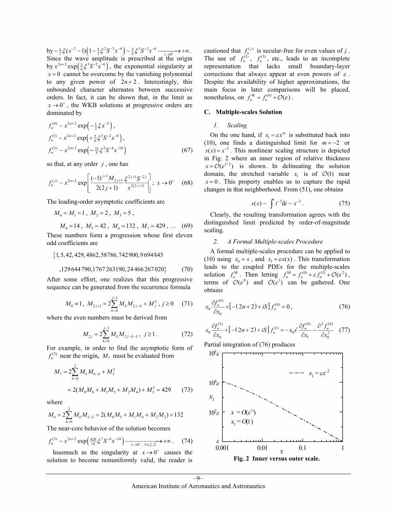
2( )s x x−= . This nonlinear scaling structure is depicted in Fig. 2 where an inner region of relative thickness

1/ 2( )x ε=O is shown. In delineating the solution domain, the stretched variable 1x is of (1)O near

0x = . This property enables us to capture the rapid changes in that neighborhood. From (51), one obtains

( )s x ∼ 3 2d ~xt t x− −∫ . (75)

Clearly, the resulting transformation agrees with the distinguished limit predicted by order-of-magnitude scaling.

2. A Formal Multiple-scales Procedure A formal multiple-scales procedure can be applied to (10) using 0x x= , and 1 ( )x s xε= . This transformation leads to the coupled PDEs for the multiple-scales solution M

nf . Then letting M (0) (1) 2( )n n nf f fε ε= + +O , terms of 0( )εO and 1( )εO can be gathered. One obtains

( )[ ](0)

(0)0

0

2 2 0∂+ − + + =

∂n

nfx n iS fx

, (76)

( )[ ](1) (0) 2 (0)

(1)0 0 2

0 1 0

2 2∂ ∂ ∂′+ − + + = − −∂ ∂ ∂

n n nn

f f fx n iS f x sx x x

(77)

Partial integration of (76) produces

0.001 0.01 0.1 1ε

102ε

104ε

106ε

x = O(ε½)x1 = O(1)

x1 = εx–2

x1

x Fig. 2 Inner versus outer scale.


( )(0)0 1 1 1 0( , ) ( ) exp 2 2 lnnf x x C x n iS x= + − . (78)

Following the solvability condition given in (42) or using the generalized solution in (50), one finds

{M 2 2 212( ) exp ( 1)n

nf x x xξ+ −= − −

}2 212ln (4 3)( 1)iS x S n xξ − − − + + − (79)

V. Discussion It is a simple exercise to verify that (63), the leading-order WKB formulation shares the same dominant terms found in (79). The distinguishing features of the multiple-scales formulation are numerous. For example, it can be argued that a) it is easy to construct, b) it is sufficiently accurate over a wide range of physical parameters, c) it is compact, and d) it reveals the problem’s underlying scaling composition. In hindsight, the unique variable transformation ( 2

1x xε −= ) is justified. In fact, it can be verified that traditional choices reminiscent of (32) do not lead to uniformly-valid expansions. Despite the solution’s oscillatory behavior, it appears that the asymptotic formulation is a good approximation to the exact solution over a wide range of physical parameters. For

0,n = the similarity between Mnf and E

nf is apparent in Fig. 3 where an order of magnitude variation in ε

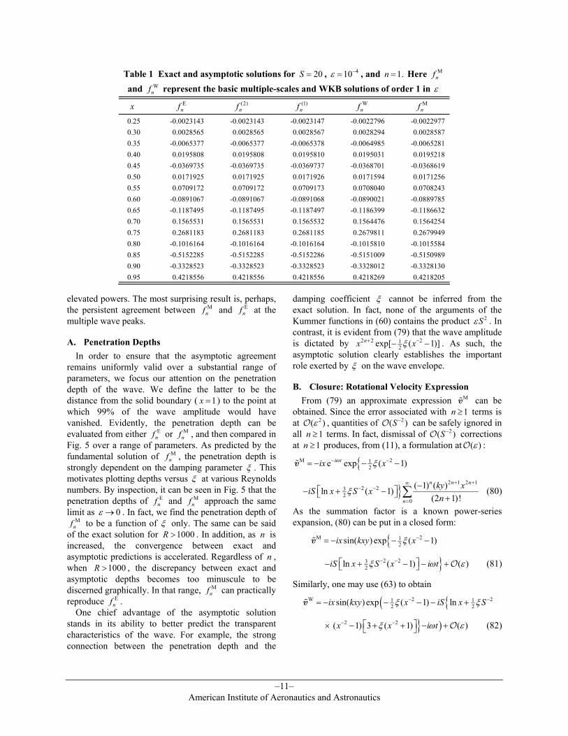
and S is illustrated. For 310ε −≤ , it becomes difficult to distinguish between exact and asymptotic solutions. Such agreement improves as R → ∞ or 0ε → . Note that the current WKB approximation deteriorates (at large ε ), when S R∼ . However, the multiple-scales solution remains more robust. This is illustrated in Fig. 3c for the case of 50S = and 100R = . A comparison between WKB and multiple-scales solutions is furnished in Table 1 for typical values of the physical parameters. It is gratifying to observe the agreement, often in several decimal places, between E

nf and asymptotic predictions. For better clarity, the absolute differences between exact and asymptotic results are shown in Fig. 4. Therein, the comparable level of precision associated with M

nf and Wnf can be

discerned. Unsurprisingly, the first-order WKB solution (1)

nf is seen to diverge near the origin, as predicted by (68); the corresponding region of nonuniformity is visible in the range 0.07x ≤ . This sudden singularity near the core is illusive because (1)

nf remains well-behaved and of 2( )εO everywhere else. In contrast,

Mnf , W

nf , and (2)nf maintain uniformity everywhere.

It can be verified that the asymptotic agreement with E

nf is retained at higher eigenvalues when a faster attenuation in the wave amplitude is noted. Since M

nf comprises an 2 2nx + factor in the wave amplitude, it can be inferred that, as 0x → , 2 2 0nx + → more rapidly at

-1.0

-0.5

0.0

0.5

1.0

ε = 10–2

S = 10

f0

a)

f0E

f0W

f0M

b)ε = 10–2

S = 20

0 0.2 0.4 0.6 0.8 1-1.0

-0.5

0.0

0.5

1.0c)

x

f0

ε = 10–2

S = 50

0.9 1

1

0 0.2 0.4 0.6 0.8 1

d)

x

ε = 10–3

S = 50

0.9 1-1

1

Fig. 3 A comparison of exact ( Ef ) with asymptotic WKB ( Wf ) and multiple-scales ( Mf ) solutions. For

210ε −= , we vary S from a) 10, to b) 20, and c) 50. Keeping 50S = , decreasing ε by one order of magnitude to 310− in d) causes results to become hardly discernable. Insets are used to show enlargements.


elevated powers. The most surprising result is, perhaps, the persistent agreement between M

nf and Enf at the

multiple wave peaks.

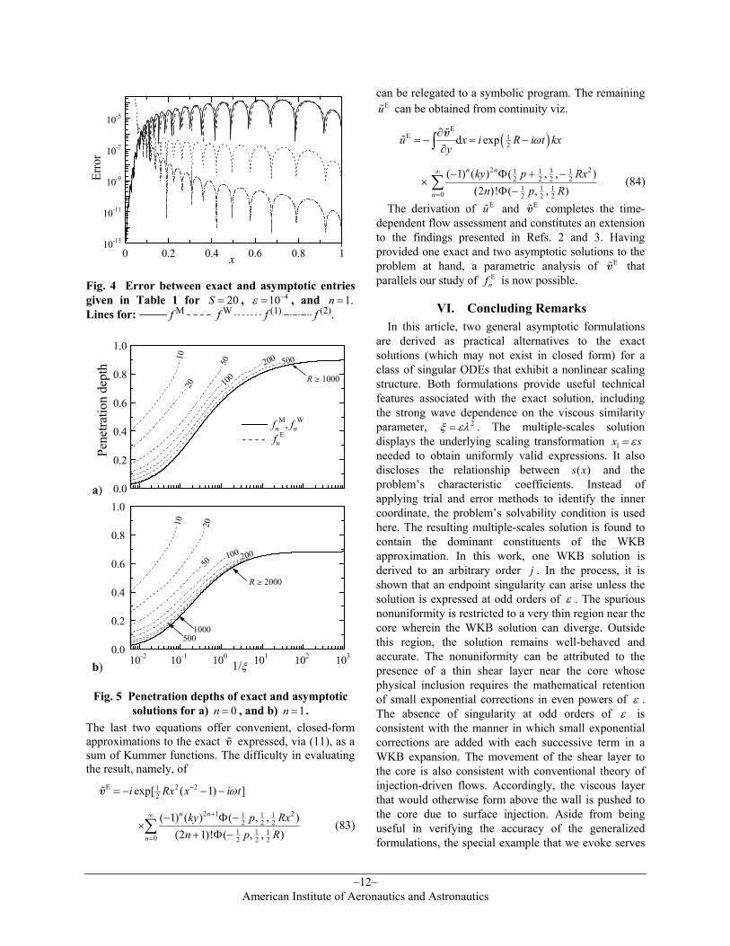
A. Penetration Depths In order to ensure that the asymptotic agreement remains uniformly valid over a substantial range of parameters, we focus our attention on the penetration depth of the wave. We define the latter to be the distance from the solid boundary ( 1x = ) to the point at which 99% of the wave amplitude would have vanished. Evidently, the penetration depth can be evaluated from either E

nf or Mnf , and then compared in

Fig. 5 over a range of parameters. As predicted by the fundamental solution of M

nf , the penetration depth is strongly dependent on the damping parameter ξ . This motivates plotting depths versus ξ at various Reynolds numbers. By inspection, it can be seen in Fig. 5 that the penetration depths of E

nf and Mnf approach the same

limit as 0ε → . In fact, we find the penetration depth of M

nf to be a function of ξ only. The same can be said of the exact solution for 1000R > . In addition, as n is increased, the convergence between exact and asymptotic predictions is accelerated. Regardless of n , when 1000R > , the discrepancy between exact and asymptotic depths becomes too minuscule to be discerned graphically. In that range, M

nf can practically reproduce E

nf . One chief advantage of the asymptotic solution stands in its ability to better predict the transparent characteristics of the wave. For example, the strong connection between the penetration depth and the

damping coefficient ξ cannot be inferred from the exact solution. In fact, none of the arguments of the Kummer functions in (60) contains the product 2Sε . In contrast, it is evident from (79) that the wave amplitude is dictated by 2 2 21

2exp[ ( 1)]ξ+ −− −nx x . As such, the asymptotic solution clearly establishes the important role exerted by ξ on the wave envelope.

B. Closure: Rotational Velocity Expression From (79) an approximate expression Mv can be obtained. Since the error associated with 1n ≥ terms is at 2( )εO , quantities of 2( )S −O can be safely ignored in all 1n ≥ terms. In fact, dismissal of 2( )S −O corrections at 1n ≥ produces, from (11), a formulation at ( )εO :

{M 212e exp ( 1)i tix xω ξ− −= − − −v

}2 1 2 1

2 232

0

( 1) ( )ln ( 1)(2 1)!

n n n

n

ky xiS x S xn

ξ+ +∞

− −

=

− − + − +∑ (80)

As the summation factor is a known power-series expansion, (80) can be put in a closed form:

{M 212sin( ) exp ( 1)ix kxy xξ −= − − −v

}2 232ln ( 1) ( )iS x S x i tξ ω ε− − − + − − + O (81)

Similarly, one may use (63) to obtain

( {W 2 21 12 2sin( ) exp ( 1) lnix kxy x iS x Sξ ξ− −= − − − − +v

} )2 2( 1) 3 ( 1) ( )x x i tξ ω ε− − × − + + − + O (82)

Table 1 Exact and asymptotic solutions for 20S = , 410ε −= , and 1.n = Here Mnf

and Wnf represent the basic multiple-scales and WKB solutions of order 1 in ε

x Enf (2)

nf (1)nf W

nf Mnf

0.25 -0.0023143 -0.0023143 -0.0023147 -0.0022796 -0.0022977 0.30 0.0028565 0.0028565 0.0028567 0.0028294 0.0028587 0.35 -0.0065377 -0.0065377 -0.0065378 -0.0064985 -0.0065281 0.40 0.0195808 0.0195808 0.0195810 0.0195031 0.0195218 0.45 -0.0369735 -0.0369735 -0.0369737 -0.0368701 -0.0368619 0.50 0.0171925 0.0171925 0.0171926 0.0171594 0.0171256 0.55 0.0709172 0.0709172 0.0709173 0.0708040 0.0708243 0.60 -0.0891067 -0.0891067 -0.0891068 -0.0890021 -0.0889785 0.65 -0.1187495 -0.1187495 -0.1187497 -0.1186399 -0.1186632 0.70 0.1565531 0.1565531 0.1565532 0.1564476 0.1564254 0.75 0.2681183 0.2681183 0.2681185 0.2679811 0.2679949 0.80 -0.1016164 -0.1016164 -0.1016164 -0.1015810 -0.1015584 0.85 -0.5152285 -0.5152285 -0.5152286 -0.5151009 -0.5150989 0.90 -0.3328523 -0.3328523 -0.3328523 -0.3328012 -0.3328130 0.95 0.4218556 0.4218556 0.4218556 0.4218269 0.4218205


The last two equations offer convenient, closed-form approximations to the exact v expressed, via (11), as a sum of Kummer functions. The difficulty in evaluating the result, namely, of

E 2 212exp[ ( 1) ]i Rx x i tω−= − − −v

2 1 21 1 1

2 2 21 1 1

0 2 2 2

( 1) ( ) ( , , )(2 1)! ( , , )

n n

n

ky p Rxn p R

+∞

=

− Φ −×

+ Φ −∑ (83)

can be relegated to a symbolic program. The remaining Eu can be obtained from continuity viz.

( )E

E 12d expu x i R i t kx

yω∂

= − = −∂∫v

2 231 1 1

2 2 2 21 1 1

0 2 2 2

( 1) ( ) ( , , )

(2 )! ( , , )

n n

n

ky p Rxn p R

∞

=

− Φ + −×

Φ −∑ (84)

The derivation of Eu and Ev completes the time-dependent flow assessment and constitutes an extension to the findings presented in Refs. 2 and 3. Having provided one exact and two asymptotic solutions to the problem at hand, a parametric analysis of Ev that parallels our study of E

nf is now possible.

VI. Concluding Remarks In this article, two general asymptotic formulations are derived as practical alternatives to the exact solutions (which may not exist in closed form) for a class of singular ODEs that exhibit a nonlinear scaling structure. Both formulations provide useful technical features associated with the exact solution, including the strong wave dependence on the viscous similarity parameter, 2ξ ελ= . The multiple-scales solution displays the underlying scaling transformation 1 ε=x s needed to obtain uniformly valid expressions. It also discloses the relationship between ( )s x and the problem’s characteristic coefficients. Instead of applying trial and error methods to identify the inner coordinate, the problem’s solvability condition is used here. The resulting multiple-scales solution is found to contain the dominant constituents of the WKB approximation. In this work, one WKB solution is derived to an arbitrary order j . In the process, it is shown that an endpoint singularity can arise unless the solution is expressed at odd orders of ε . The spurious nonuniformity is restricted to a very thin region near the core wherein the WKB solution can diverge. Outside this region, the solution remains well-behaved and accurate. The nonuniformity can be attributed to the presence of a thin shear layer near the core whose physical inclusion requires the mathematical retention of small exponential corrections in even powers of ε . The absence of singularity at odd orders of ε is consistent with the manner in which small exponential corrections are added with each successive term in a WKB expansion. The movement of the shear layer to the core is also consistent with conventional theory of injection-driven flows. Accordingly, the viscous layer that would otherwise form above the wall is pushed to the core due to surface injection. Aside from being useful in verifying the accuracy of the generalized formulations, the special example that we evoke serves

0 0.2 0.4 0.6 0.8 110-13

10-11

10-9

10-7

10-5

Erro

r

x

Fig. 4 Error between exact and asymptotic entries given in Table 1 for 20S = , 410ε −= , and 1.n =Lines for: f M f W f (1) f (2).

0.0

0.2

0.4

0.6

0.8

1.0

Pene

tratio

n de

pth

a)

R ¥ 1000

500200

100

50

2010

fnM, fn

W

- - - - fnE

10-2 10-1 100 101 102 1030.0

0.2

0.4

0.6

0.8

1.0

1000

b)

R ¥ 2000

500

20010050

2010

1/ξ

Fig. 5 Penetration depths of exact and asymptotic solutions for a) 0n = , and b) 1n = .


a practical purpose. It provides one exact and two asymptotic solutions to an applied study described previously in Refs. 2 and 3. Since the former work could only produce approximate solutions, the advantages of an exact solution include increased accuracy and independence of parametric size. From a perturbation standpoint, the current work reinforces the ideas presented in Ref. 33 regarding the manner in which scales can be selected. For example, the freedom in the present selection of the inner variable transformation increases our repertory of scaling choices. We hope that the rigorous specification of the undetermined scale functional may be used in similar boundary-value problems.

References 1Majdalani, J., “Vorticity Dynamics in Isobarically Closed Porous Channels. Part 1: Standard Perturbations,” Journal of Propulsion and Power, Vol. 17, No. 2, 2001, pp. 355-362. 2Majdalani, J., “Asymptotic Formulation for an Acoustically Driven Field inside a Rectangular Cavity with a Well-Defined Convective Mean Flow Motion,” Journal of Sound and Vibration, Vol. 223, No. 1, 1999, pp. 73-95. 3Majdalani, J., “Vortical and Acoustical Mode Coupling inside a Two-Dimensional Cavity with Transpiring Walls,” Journal of the Acoustical Society of America, Vol. 106, No. 1, 1999, pp. 46-56. 4Flandro, G. A., “Effects of Vorticity Transport on Axial Acoustic Waves in a Solid Propellant Rocket Chamber,” Combustion Instabilities Driven by Thermo-Chemical Acoustic Sources, NCA Vol. 4, American Society of Mechanical Engineers, New York, 1989, pp. 53-61. 5Flandro, G. A., “Effects of Vorticity on Rocket Combustion Stability,” Journal of Propulsion and Power, Vol. 11, No. 4, 1995, pp. 607-625. 6Flandro, G. A., Cai, W., and Yang, V., “Turbulent Transport in Rocket Motor Unsteady Flowfield,” Solid Propellant Chemistry, Combustion, and Motor Interior Ballistics, Vol. 185, edited by V. Yang, T. B. Brill, and W.-Z. Ren, AIAA Progress in Astronautics and Aeronautics, Washington, DC, 2000, pp. 837-858. 7Majdalani, J., and Van Moorhem, W. K., “Improved Time-Dependent Flowfield Solution for Solid Rocket Motors,” AIAA Journal, Vol. 36, No. 2, 1998, pp. 241-248. 8Majdalani, J., “The Boundary Layer Structure in Cylindrical Rocket Motors,” AIAA Journal, Vol. 37, No. 4, 1999, pp. 505-508. 9Terrill, R. M., “Laminar Flow in a Uniformly Porous Channel with Large Injection,” The Aeronautical Quarterly, Vol. 16, 1965, pp. 323-332. 10Berman, A. S., “Laminar Flow in Channels with Porous Walls,” Journal of Applied Physics, Vol. 24, No. 9, 1953, pp. 1232-1235.

11Yuan, S. W., “Further Investigation of Laminar Flow in Channels with Porous Walls,” Journal of Applied Physics, Vol. 27, No. 3, 1956, pp. 267-269. 12Barron, J., Majdalani, J., and Van Moorhem, W. K., “A Novel Investigation of the Oscillatory Field over a Transpiring Surface,” Journal of Sound and Vibration, Vol. 235, No. 2, 2000, pp. 281-297. 13Beddini, R. A., “Injection-Induced Flows in Porous-Walled Ducts,” AIAA Journal, Vol. 24, No. 11, 1986, pp. 1766-1773. 14Beddini, R. A., and Roberts, T. A., “Turbularization of an Acoustic Boundary Layer on a Transpiring Surface,” AIAA Journal, Vol. 26, No. 8, 1988, pp. 917-923. 15Hino, M., Sawamoto, M., and Takasu, S., “Experiments on Transition to Turbulence in an Oscillatory Pipe Flow,” Journal of Fluid Mechanics, Vol. 75, 1976, pp. 193-207. 16Hino, M., Kashiwayanagi, M., Nakayama, A., and Hara, T., “Experiments on the Turbulence Statistics and the Structure of a Reciprocating Oscillatory Flow,” Journal of Fluid Mechanics, Vol. 131, 1983, pp. 193-207. 17Hino, M., Fukunishi, Y., and Meng, Y., “Experimental Study of a Three-Dimensional Large-Scale Structure in a Reciprocating Oscillatory Flow,” Fluid Dynamics Research, Vol. 6, 1990, pp. 261-275. 18Hasebe, M., Hino, M., and Hoshi, K., “Flood Forecasting by the Filter Separation Ar Method and Comparison with Modeling Efficiencies by Some Rainfall-Runoff Models,” Journal of Hydrology, Vol. 110, 1989, pp. 107-136. 19Peng, Y., and Yuan, S. W., “Laminar Pipe Flow with Mass Transfer Cooling,” Journal of Heat Transfer, Vol. 87, No. 2, 1965, pp. 252-258. 20Skalak, F. M., and Wang, C.-Y., “On the Nonunique Solutions of Laminar Flow through a Porous Tube or Channel,” SIAM Journal on Applied Mathematics, Vol. 34, No. 3, 1978, pp. 535-544. 21Shih, K.-G., “On the Existence of Solutions of an Equation Arising in the Theory of Laminar Flow in a Uniformly Porous Channel with Injection,” SIAM Journal on Applied Mathematics, Vol. 47, No. 3, 1987, pp. 526-533. 22Zaturska, M. B., Drazin, P. G., and Banks, W. H. H., “On the Flow of a Viscous Fluid Driven Along a Channel by Suction at Porous Walls,” Fluid Dynamics Research, Vol. 4, No. 3, 1988, pp. 151-178. 23Cox, S. M., “Two-Dimensional Flow of a Viscous Fluid in a Channel with Porous Walls,” Journal of Fluid Mechanics, Vol. 227, 1991, pp. 1-33. 24Taylor, C. L., Banks, W. H. H., Zaturska, M. B., and Drazin, P. G., “Three-Dimensional Flow in a Porous Channel,” Quarterly Journal of Mechanics and Applied Mathematics, Vol. 44, No. 1, 1991, pp. 105-133. 25Hastings, S. P., Lu, C., and MacGillivray, A. D., “A Boundary Value Problem with Multiple Solutions from the Theory of Laminar Flow,” SIAM Journal on Mathematical Analysis, Vol. 23, No. 1, 1992, pp. 201-208.


26Lu, C., “On the Asymptotic Solution of Laminar Channel Flow with Large Suction,” SIAM Journal on Mathematical Analysis, Vol. 28, No. 5, 1997, pp. 1113-1134. 27Lu, C., MacGillivray, A. D., and Hastings, S. P., “Asymptotic Behaviour of Solutions of a Similarity Equation for Laminar Flows in Channels with Porous Walls,” IMA Journal of Applied Mathematics, Vol. 49, 1992, pp. 139-162. 28MacGillivray, A. D., and Lu, C., “Asymptotic Solution of a Laminar Flow in a Porous Channel with Large Suction: A Nonlinear Turning Point Problem,” Methods and Applications of Analysis, Vol. 1, No. 2, 1994, pp. 229-248. 29Robinson, W. A., “The Existence of Multiple Solutions for the Laminar Flow in a Uniformly Porous Channel with Suction at Both Walls,” Journal of Engineering Mathematics, Vol. 10, No. 1, 1976, pp. 23-40. 30Terrill, R. M., “Laminar Flow in a Uniformly Porous Channel,” The Aeronautical Quarterly, Vol. 15, 1964, pp. 299-310. 31Terrill, R. M., and Shrestha, G. M., “Laminar Flow through Parallel and Uniformly Porous Walls of Different Permeability,” Journal of Applied Mathematics and Physics,

Vol. 16, 1965, pp. 470-482. 32Potter, M. C., and Foss, J. F., Fluid Mechanics, Great Lakes Press Inc., Okemos, 1982, pp. 368-369. 33Majdalani, J., “A Hybrid Multiple Scale Procedure for Boundary Layers Involving Several Dissimilar Scales,” Journal of Applied Mathematics and Physics, Vol. 49, No. 6, 1998, pp. 849-868. 34Bender, C. M., and Orszag, S. A., Advanced Mathematical Methods for Scientists and Engineers, McGraw-Hill Book Company Inc., New York, 1978. 35Zhao, Q., Staab, P. L., Kassoy, D. R., and Kirkköprü, K., “Acoustically Generated Vorticity in an Internal Flow,” Journal of Fluid Mechanics, Vol. 413, No. 25, 2000, pp. 247-285. 36Staab, P. L., and Kassoy, D. R., “Three-Dimensional, Unsteady, Acoustic-Shear Flow Dynamics in a Cylinder with Sidewall Mass Addition,” Physics of Fluids, Series B, Vol. 9, 1996, pp. 3753-3763. 37Gradshtein, I. S., and Ryzhik, I. M., Table of Integrals, Series, and Products, 5th ed., edited by J. Alan, Academic Press, Boston, 1994, pp. 1084-1096.

aiaa 2002-2985

Documents