ai-sesi04 searching (heuristic search) · pdf fileheuristic search pertemuan : 4 ... dynamic...
TRANSCRIPT
IF-UTAMA 1
IF-UTAMA 1
Jurusan Teknik Informatika – Universitas Widyatama
Heuristic Search
Pertemuan : 4
Dosen Pembina :
Sriyani Violina
Danang Junaedi
IF-UTAMA 2
• Deskripsi
• Heuristic Search– Simulated Annealing
– Simplified Memory Bounded A*
– Bi-Directional A*
– Modified Bi-Directional A*
– Dynamic Weighthing A*
Overview

IF-UTAMA 2
IF-UTAMA 3
• Pertemuan ini mempelajari bagaimana
memecahkan suatu masalah dengan teknik
searching.
• Metode searching yang dibahas pada pertemuan
ini adalah heuristic search atau informed search
yang terdiri dari:– Simulated Annealing
– Simplified Memory Bounded A*
– Bi-Directional A*
– Modified Bi-Directional A*
– Dynamic Weighthing A*
Deskripsi
IF-UTAMA 4
Simulated Annealing
• A alternative to a random-restart hill-climbing when stuck
on a local maximum is to do a ‘reverse walk’ to escape
the local maximum.
• This is the idea of simulated annealing.
• The term simulated annealing derives from the roughly
analogous physical process of heating and then slowly
cooling a substance to obtain a strong crystalline
structure.
• The simulated annealing process lowers the temperature
by slow stages until the system ``freezes" and no further
changes occur.

IF-UTAMA 3
IF-UTAMA 5
Search using Simulated Annealing
• Simulated Annealing = hill-climbing with non-deterministic
search
• Basic ideas:
– like hill-climbing identify the quality of the local improvements
– instead of picking the best move, pick one randomly
– say the change in objective function is δ
– if δ is positive, then move to that state
– otherwise:
• move to this state with probability proportional to δ
• thus: worse moves (very large negative δ) are executed less often
– however, there is always a chance of escaping from local maxima
– over time, make it less likely to accept locally bad moves
– (Can also make the size of the move random as well, i.e., allow
“large” steps in state space)
IF-UTAMA 6
Physical Interpretation of Simulated
Annealing
• A Physical Analogy:• imagine letting a ball roll downhill on the function surface
– this is like hill-climbing (for minimization)
• now imagine shaking the surface, while the ball rolls, gradually
reducing the amount of shaking
– this is like simulated annealing
• Annealing = physical process of cooling a liquid or
metal until particles achieve a certain frozen crystal
state• simulated annealing:
– free variables are like particles
– seek “low energy” (high quality) configuration
– get this by slowly reducing temperature T, which particles move
around randomly

IF-UTAMA 4
IF-UTAMA 7
Simulated Annealing
• Probability of transition to higher energy
state is given by function:
– P = e –∆E/kt
Where ∆E is the positive change in the energy level
T is the temperature
K is Boltzmann constant.
IF-UTAMA 8
Differences
• The algorithm for simulated annealing is
slightly different from the simple-hill
climbing procedure. The three differences
are:
– The annealing schedule must be maintained
– Moves to worse states may be accepted
– It is good idea to maintain, in addition to the
current state, the best state found so far.

IF-UTAMA 5
IF-UTAMA 9
Algorithm: Simulate Annealing
1. Evaluate the initial state. If it is also a goal state, then return it and quit. Otherwise, continue with the initial state as the current state.
2. Initialize BEST-SO-FAR to the current state.
3. Initialize T according to the annealing schedule
4. Loop until a solution is found or until there are no new operators left to be applied in the current state.
a. Select an operator that has not yet been applied to the current state and apply it to produce a new state.
b. Evaluate the new state. Compute:• ∆E = ( value of current ) – ( value of new state)
• If the new state is a goal state, then return it and quit.
• If it is a goal state but is better than the current state, then make it the current state. Also set BEST-SO-FAR to this new state.
• If it is not better than the current state, then make it the current state with probability p’ as defined above. This step is usually implemented by invoking a random number generator to produce a number in the range [0, 1]. If the number is less than p’, then the move is accepted. Otherwise, do nothing.
c. Revise T as necessary according to the annealing schedule
5. Return BEST-SO-FAR as the answer
IF-UTAMA 10
Simulate Annealing: Implementation
• It is necessary to select an annealing schedule
which has three components:
– Initial value to be used for temperature
– Criteria that will be used to decide when the
temperature will be reduced
– Amount by which the temperature will be
reduced.

IF-UTAMA 6
IF-UTAMA 11
• To address complex search problems, we often put constraints on memory requirements.
• We will examine two algorithms: (a) IDA* search and (b) SMA* search.
• Iterative Deepening A* Search (IDA*) uses a DFS for every iteration where an f-cost limit is used instead of a depth limit.
• Each iteration expands all the nodes that lie inside a contour for the current f-cost.
• The time complexity depends on the different values that the heuristic can take on.
• IDA* is complete, optimal, and memory-bounded.
• To improve IDA*, we often increase the f-cost limit by a fixed amount ε on each iteration. Such an approach is called ε-admissible.
Memory Bounded Search
IF-UTAMA 12
SIMPLIFIED MEMORY-BOUNDED A*
(SMA*)
• IDA* cannot remember its previous steps since it uses too little memory (between iterations only the f-cost limit is kept).
• If the state space is graph, IDA* often repeats itself.
• Uses all available memory for the search– drops nodes from the queue when it runs out of space
• those with the highest f-costs
– If there is a tie (equal f-values) we first delete the oldest nodes first.
– complete if there is enough memory for the shortest solution path
– often better than A* and IDA*• but some problems are still too tough
• trade-off between time and space requirements
• It is complete and optimal if the available memory allows SMA* to store the shallowest solution path.
• When enough memory is available for the whole search tree, the search is optimally efficient.
12
IF-UTAMA 7
IF-UTAMA 13
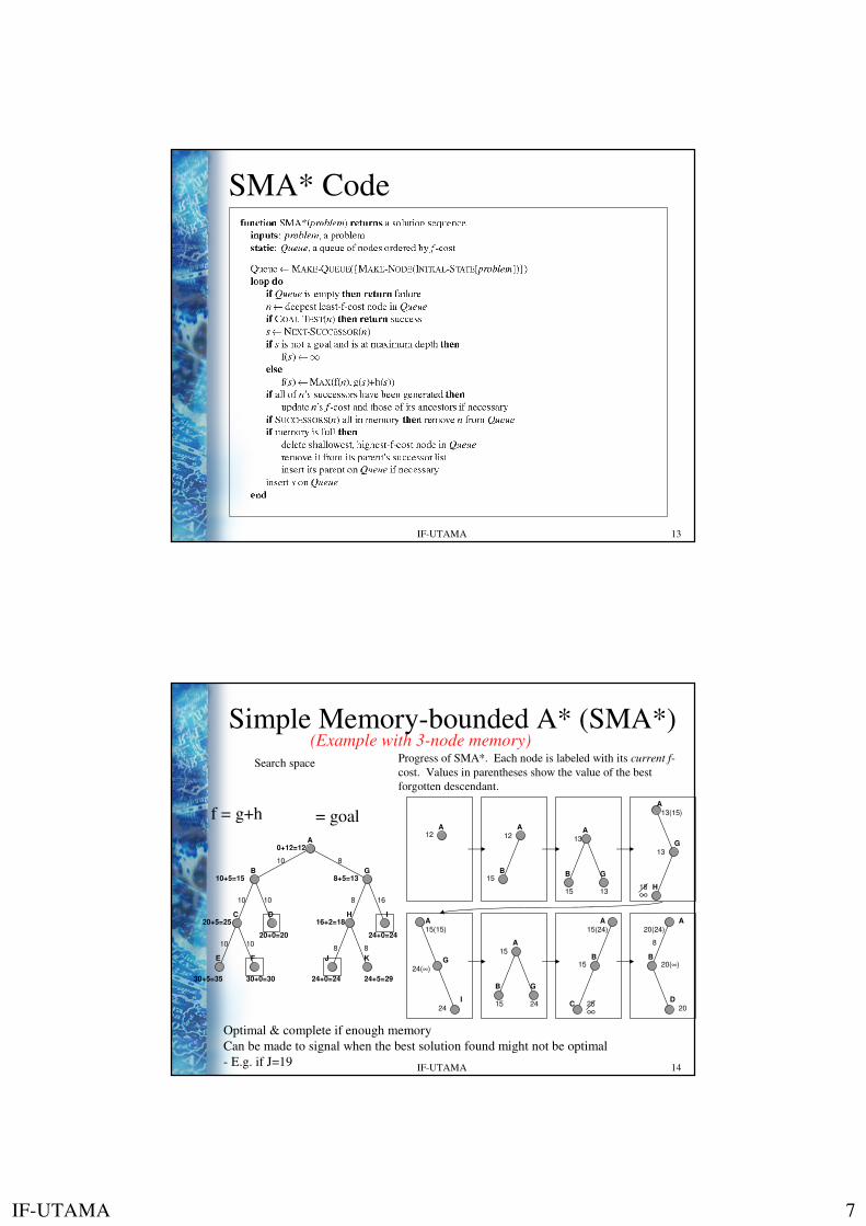
SMA* Code
IF-UTAMA 14
Simple Memory-bounded A* (SMA*)
24+0=24
A
B G
C D
E F
H
J
I
K
0+12=12
10+5=15
20+5=25
30+5=35
20+0=20
30+0=30
8+5=13
16+2=18
24+0=24 24+5=29
10 8
10 10
10 10
8 16
8 8
A
12A
B
12
15
A
B G
13
15 13H
13
∞
A
G
18
13(15)
A
G
24(∞)
I
15(15)
24
A
B G
15
15 24
∞
A
B
C
15(24)
15
25
f = g+h
(Example with 3-node memory)
A
B
D
8
20
20(24)
20(∞)
Progress of SMA*. Each node is labeled with its current f-
cost. Values in parentheses show the value of the best
forgotten descendant.
Optimal & complete if enough memory
Can be made to signal when the best solution found might not be optimal
- E.g. if J=19
� = goal
Search space

IF-UTAMA 8
IF-UTAMA 15
Ex: Rute Perjalanan
10
10
80
10
35
70203010040070748570608080h(n)
607050254590205302515100b(n)
MLKJHGFEDCBASn
h(n):heuristic jarak antar suatu kota dan b(n):perkiraan biaya menuju kota asal
IF-UTAMA 16
Solusi SMA*
IF-UTAMA 9
IF-UTAMA 17
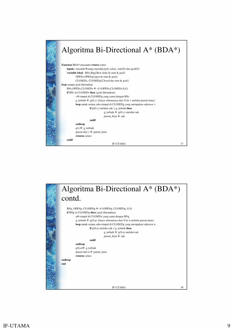
Algoritma Bi-Directional A* (BDA*)
Function BDA*(masalah) return solusi
inputs: masalah�ruang masalah,jenis solusi, start(S) dan goal(G)
variable lokal : BNs,Bng{Best node dr start & goal}
OPENs,OPENg{open dr start & goal}
CLOSEDs, CLOSEDg{Closed dar start & goal}
loop sampai goal ditemukan
BNs,OPENs,CLOSEDs A*(OPENs,CLOSEDs,S,G)
if BNs in CLOSEDs then {goal ditemukan}
vsimpul di CLOSEDg yang sama dengan BNs
g_terbaik g(G,v) {biaya sebenarnya dari G ke v melalui parent lama}
loop untuk semua suk=simpul di CLOSEDg yang merupakan suksesor v
if g(G,v) melalui suk < g_terbaik then
g_terbaik g(G,v) melalui suk
parent_baru suk
endif
endloop
g(v) g_terbaik
parent dari v parent_baru
returns solusi
endif
IF-UTAMA 18
Algoritma Bi-Directional A* (BDA*)
contd.BNg, OPENg, CLOSEDg A*(OPENg, CLOSEDg, G,S)
if BNg in CLOSEDg then {goal ditemukan}
usimpul di CLOSEDs yang sama dengan BNg
g_terbaik g(S,u) {biaya sebenarnya dari S ke u melalui parent lama}
loop untuk semua suk=simpul di CLOSEDg yang merupakan suksesor u
if g(S,u) melalui suk < g_terbaik then
g_terbaik g(S,u) melalui suk
parent_baru suk
endif
endloop
g(S,u) g_terbaik
parent dari u parent_baru
returns solusi
endloop
end

IF-UTAMA 10
IF-UTAMA 19
Solusi Bi-Directional A*
IF-UTAMA 20
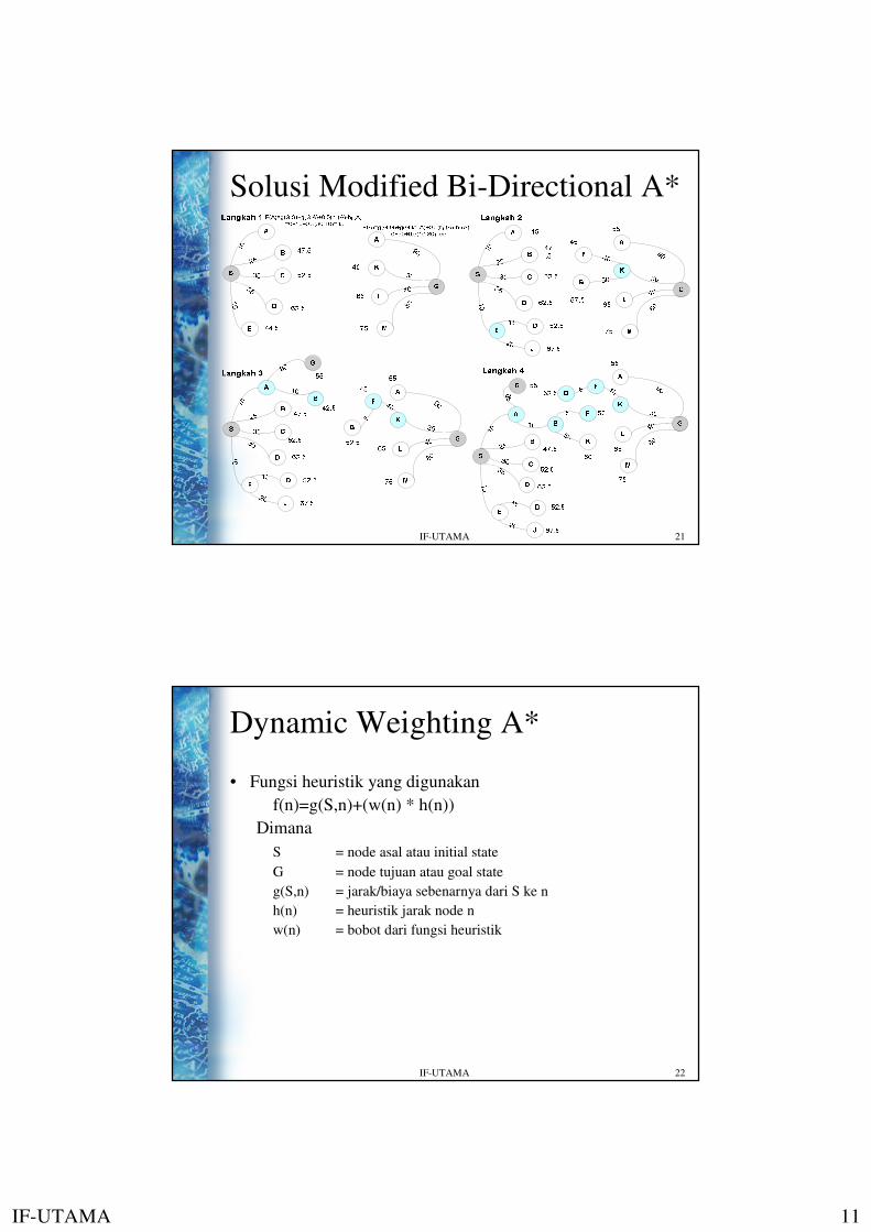
Modified Bi-Directional A*
• Yang dimodifikasi adalah fungsi heuristiknya menjadi
– Untuk pencarian maju
f(n)=g(S,n) + 0.5 * (h(n) - b(n))
– Untuk pencarian mundur
f(n)=g(G,n) + 0.5 * (b(n) - h(n))
Dimana
S = node asal atau initial state
G = node tujuan atau goal state
g(S,n) = jarak/biaya sebenarnya dari S ke n
g(G,n) = jarak/biaya sebenarnya dari G ke n
h(n) = heuristik jarak node n
b(n) = heuristik biaya node n
IF-UTAMA 11
IF-UTAMA 21
Solusi Modified Bi-Directional A*
IF-UTAMA 22
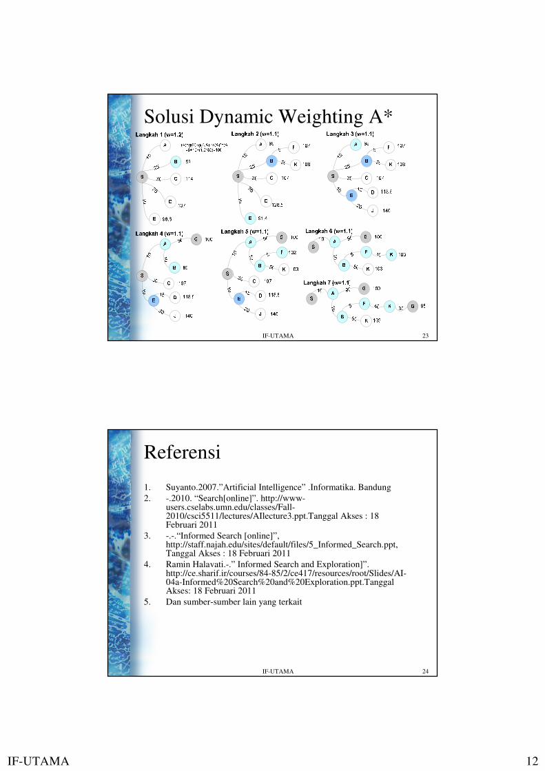
Dynamic Weighting A*
• Fungsi heuristik yang digunakan
f(n)=g(S,n)+(w(n) * h(n))
Dimana
S = node asal atau initial state
G = node tujuan atau goal state
g(S,n) = jarak/biaya sebenarnya dari S ke n
h(n) = heuristik jarak node n
w(n) = bobot dari fungsi heuristik
IF-UTAMA 12
IF-UTAMA 23
Solusi Dynamic Weighting A*
IF-UTAMA 24
Referensi
1. Suyanto.2007.”Artificial Intelligence” .Informatika. Bandung
2. -.2010. “Search[online]”. http://www-users.cselabs.umn.edu/classes/Fall-2010/csci5511/lectures/AIlecture3.ppt.Tanggal Akses : 18 Februari 2011
3. -.-.“Informed Search [online]”, http://staff.najah.edu/sites/default/files/5_Informed_Search.ppt, Tanggal Akses : 18 Februari 2011
4. Ramin Halavati.-.” Informed Search and Exploration]”. http://ce.sharif.ir/courses/84-85/2/ce417/resources/root/Slides/AI-04a-Informed%20Search%20and%20Exploration.ppt.Tanggal Akses: 18 Februari 2011
5. Dan sumber-sumber lain yang terkait