a.i. alikhanyan national science laboratory (yerevan...
TRANSCRIPT

A study of charged hadron yields and the multidimensional nuclear
attenuation effect at the HERMES experiment
DISSERTATION
A.I. Alikhanyan National Science Laboratory
(Yerevan Physics Institute)
Karyan Gevorg Ararat
Thesis for acquiring the degree of candidate of physical and
mathematical sciences in division 01.04.16 "nuclear, elementary
particles and cosmic ray physics"
Scientific supervisor:
doctor of physical and mathematical sciences, professor N.Z. Akopov
Contents
Contents i
Introduction iii
1 Physics Motivation 1
1.1 Deep-Inelastic Scattering( DIS ) . . . . . . . . . . . . . . . . . . . . . . . . . . . 1
1.2 Hadronization in Nuclear Enviorement . . . . . . . . . . . . . . . . . . . . . . . 6
1.2.1 The Two-Scale Model . . . . . . . . . . . . . . . . . . . . . . . . . . . . . 8
1.2.2 Gluon Bremmstrahlung Model( GBM ) . . . . . . . . . . . . . . . . . . . 11
1.2.3 Rescaling Models( RM ) . . . . . . . . . . . . . . . . . . . . . . . . . . . 13
1.2.4 BUU (Boltzmann-Uehling-Uhlenbeck) Transport Model . . . . . . . . . . 14
2 The HERMES Experiment 16
2.1 The target system . . . . . . . . . . . . . . . . . . . . . . . . . . . . . . . . . . . 17
2.2 The HERMES spectrometer . . . . . . . . . . . . . . . . . . . . . . . . . . . . . 17
2.2.1 The Spectrometer Magnet . . . . . . . . . . . . . . . . . . . . . . . . . . 18
2.2.2 Tracking Detectors . . . . . . . . . . . . . . . . . . . . . . . . . . . . . . 18
2.2.3 Particle Identification (PID) . . . . . . . . . . . . . . . . . . . . . . . . . 20
2.2.4 The RICH Detector . . . . . . . . . . . . . . . . . . . . . . . . . . . . . . 21
2.2.5 The PID Algorithm . . . . . . . . . . . . . . . . . . . . . . . . . . . . . . 22
2.2.6 The HERMES Luminosity Measurement . . . . . . . . . . . . . . . . . . 24
2.3 Data Analysis . . . . . . . . . . . . . . . . . . . . . . . . . . . . . . . . . . . . . 24
2.3.1 Data Selection . . . . . . . . . . . . . . . . . . . . . . . . . . . . . . . . . 25
2.4 The RICH Unfolding . . . . . . . . . . . . . . . . . . . . . . . . . . . . . . . . . 26
2.5 Charged Hadron Yields . . . . . . . . . . . . . . . . . . . . . . . . . . . . . . . . 28
2.5.1 Charge Symmetric Background . . . . . . . . . . . . . . . . . . . . . . . 33
2.6 The HERMES Monte Carlo Package . . . . . . . . . . . . . . . . . . . . . . . . 34
2.6.1 Event Generators . . . . . . . . . . . . . . . . . . . . . . . . . . . . . . . 36
2.6.2 Unfolding for Radiative Effects and Detector Smearing . . . . . . . . . . 37
i

CONTENTS
3 Results and Conclusions 40
3.1 ν dependence in three z slices . . . . . . . . . . . . . . . . . . . . . . . . . . . . 40
3.2 z dependence in three ν slices . . . . . . . . . . . . . . . . . . . . . . . . . . . . 59
3.3 p2t dependence in three z slices . . . . . . . . . . . . . . . . . . . . . . . . . . . 78
3.4 z dependence in three p2t slices . . . . . . . . . . . . . . . . . . . . . . . . . . . 88
3.5 Conclusion . . . . . . . . . . . . . . . . . . . . . . . . . . . . . . . . . . . . . . . 106
References 109
ii

Introduction
Many centuries people were struggling to explain what everything around us is made of. It
is not strange that the first debates on this held in Greece in one of the ancient centers of human
civilization. The story starts with Thales(624 - 546 B.C.) from Miletus whose philosophy of
nature based on the fundamental doctrine that water was the basis of all life and everything
was made of water. As Arystotle says later "Of those who first philosophized the majority
assumed only material principles or elements, Thales, the originator of such philosophy, taking
water for his principle". This was the challenging achievement since he was the first, whome
explanation of the world has shown scientific tendency based on "atomistic" view of everything
in contrast with the ancient poets whose interpretations about the world were based on the
mythical things.
The idea of the "atomistic" world then was developed by Anaximander(610 - 546 B.C.),
the disciple of Thales, who also believed that all things originated from one original material
element, the principle, but in opposition to his teacher, Anaximander assumed that this princi-
ple is undetermined in quality and infinite in quantity and he called it the aperion, translated
as "limitless".
Then the disciple of Anaximander, the Anaximenes(585 - 528 B.C.) of Miletus, formulated
his concept of the world based on the air as the first principle and fire, wind, clouds, water and
earth produced from it by condensation and rarefaction.
But the "atomistic" ideas of Thales about the nature of matter around us were philosoph-
ically crystallized in 180 years later in works of Leucippus and Democritus(460 - 370 B.C) from
Abdera who were known as the founders of the atomistic philosophy. As the Democritus quotes
the Leucippus "The atomists hold that splitting stops when it reaches indivisible particles and
iii

does not go on infinitely." The idea of the Democritus was based on a logic that if a matter
could be infinitely divided, then it can never be put back together. Although a matter can be
destroyed, it can also put back together by joining a simpler pieces which means the process
of disintegration and reintegration is reversible. Hence, there must be a lower limit for the
splitting of matter, otherwise it can be split infinitely, and nothing will be able to stop it from
going on forever and destroying all matter.
The modern era of "atomistic" ideas starts with Newton(1642 - 1727) who in his "Prin-
cipa" says " ... I am induced by many reasons to suspect that the phenomena of nature depends
on certain forces by which the particles of bodies, by some causes hitherto unknown, are ei-
ther mutually impelled towards each other cohere in regular figures, or are repelled and recede
from each other, which forces being unknown philosophers have hitherto attempted the search
of nature in vain." But still the atomic ideas were qualitative until an English chemist, John
Dalton(1766 - 1844), in 1803 gave them a quantitative form in his work of "New System of
Chemical Philosophy". The main idea of Dalton was that the atoms of the same element have
identical properties and masses. And, as a consequence, it was possible to estimate the relative
atomic weights measuring the relative combining weights of chemical elements, with various
compounds, observed in nature.
But only more than ten years later, in 1815, William Prout(1785 - 1850) had observed
that the relative atomic weights of the elements were very close to the numbers which are an
integral multiples of hydrogen atoms. Based on this observation he hypothesized that atoms
of all elements are the compounds of the hydrogen atoms. But more accurate measurements
provided later showed that many of atomic weights did not have an integral values.
In 1833 Michael Faraday(1791 - 1867) found the laws of electrolysis showing in the first
time that the electric charge is somehow associated with the atoms and also it has an atomistic
structure.
With discovery of the radioactivity, in 1896, by the French physicist Henri Becquerel(1852
- 1908), the idea of "indivisible" atom seemed to be wrong. Becquerel found that uranium salts
emit a penetrating radiation which have an influence on a photographic plate. More later, the
Ernest Rutherford(1871 - 1937) discovered that there are different kinds of radiations. Some
iv

of them are less penetrating than the rest. He called the less penetrating radiation the α rays
and the more powerful ones the β rays just using the first two letters of the Greek alphabet.
But finally the concept of "indivisible" atom broke down in 1897 when an English physicist
J.J Thomson(1856 - 1940) pronounced the discovery of the electron, a unit of the electric charge,
to be a constituent part of an atom. He calculated that the electron has to had a mass about
1837 times lighter than the mass of a hydrogen atom. In 1904, he proposed his "plum pudding"
model of atom where negatively charged electrons, the "plums", are surrounded by positively
charged "pudding", forming an electrically neutral atom.
But in 1911 Ernest Rutherford disproved Thomson’s "plum-pudding" model of an atom
in his famous gold-foil experiment where he showed that the atom has a very tiny, but massive,
positively charged core, the nucleus. He proposed his model of atom known as the dynamic
model (or planetary model in analogous with the solar sytem) according to which atoms con-
sist of the nucleus surrounded by the negatively charged electrons. According to this model
Rutherfort calculated that the angular distribution of the scattared α particles should follow to
sin−4(φ2), where φ is the scattering angle. These calculations were done assuming that nucleus
has no structure, it is a "point-like".
Continuing his experiments, in 1919, bombarding hydrogen and other light atoms with
α particles, Rutherford discovered the proton. He concluded, that positively charged parti-
cles produced in these reactions are nuclei of the hydrogen atoms. At this stage only two
fundamental particles were known: the electron and the proton.
In 1930, bombarding beryllium atoms with α particles, the German physicists Walther
Bothe(1891 - 1957) and Hans Becker(1911 - 1944) observed a neutral radiation coming from
the beryllium atoms. Then in 1932 the French physicists Frederic Juliot-Curie(1900 - 1958)
and Irene Juliot-Curie(1897 - 1956) found that this radiation could eject protons from materials
containing the hydrogen atoms.
In the same year, James Chadwick(1891 - 1974), repeated Juliot’s experiment, directing
beryllium radiation to the different materials such as lithium, beryllium and boron. He found
that protons were ejected from nuclei of these elements too. According to his calculations the
beryllium radiation was corespond to the neutral particles of approximately the same mass as
v

the proton. He had discovered the neutron.
The discovery of neutron alive the assumption proposed by the Heisenberg(1901 - 1976)
and the Ivanenko(1904 - 1994) that the atomic nucleus consists of neutrons and protons and
that the electrons in atoms are outside from the nucleus.
In 1950’s, with development of the accelarator technologies when beam energies became
much higher the deviations were observed from Rutherfort "point-like" nucleus assumption.
The pionering experiment was done by Robert Hofstadter(1915 - 1990) and colleagues using
the 125 MeV energy electron beam at the Stanford Linear Accelarator Center(SLAC). They
measured the angular distribution of elastically scattered electrons from gold and observed a
significant deviation from the "point-like" nucleus prediction. The Hofstadter and his team
explained the observation as a combination of two effects. The first effect is corresponding to
the scattering off a "point-like" target and the second effect caused by a spatial extension of
target charge density which they called a "form factor". This was the clear indication that
nucleus is not a "point-like" but has a size which they estimated to be a few fermi(1fm = 10−13
cm).
In 1964, Gell-Mann Murray and George Zweig, independently, had proposed that protons
and other hadrons( strongly interacting particles ) known at that time built from more basic
blocks, which they called "quarks". Three years later, in 1967, MIT( Massachusetts Institute
of Technology ) - SLAC collaboration performed electron-proton elastic scattering which gave
no evidence for quark substructure. In late 1967, they performed the first Deep Inelastic Scat-
tering( DIS ) experiment using 20 GeV electron beam and proton target. Data analysis showed
that a DIS cross section( interaction probability ) is decreasing very slowly with transfered four
momentum squared( Q2 ) than that for the elastic scattering. This was a clear indication of
some hard core inside a proton.
As suggested first by the Bjorken in 1967, DIS experiments might being a tool to inves-
tigate an elementary constituents of matter. Subsequently, many DIS experiments are pro-
vided(ing) in various scientific laboratories to deepen our knowledge of matter constituents and
a large variety of elementary particles.
vi

Chapter 1
Physics Motivation
1.1 Deep-Inelastic Scattering( DIS )
A simple example of deep-inelastic scattering process might be the scattering of high
energetic leptons(electrons, muons) on free nucleons, such as protons.
l(k) +N(P) → l(k′) +X (1.1)
Using an appropriate energy regime, one can suppress the weak interaction(due to the high
masses of the exchange bosons) and thus only the electromagnetic interaction will be relevant.
In one photon approximation, also known as the Born first approximation, an incoming charged
lepton with four-momentum : k( E, ~k ) interacts, via a single virtual photon, with a proton,
which in it’s rest frame characterized by a four-momentum: P( M, 0 ). A simple illustration
diagram for this process is shown in Figure 1.1.
Detecting the scattered lepton with four-momentum : k′( E′, ~k′ ), one can define the
four-momentum transfer between the lepton and the proton as : q = k - k′. Since the four-
momentum of a virtual photon is a spaclike vector we can introduce the Lorentz invariant
quantity : Q2 ≡ -q2, as a negative squared four-momentum transfer from the lepton to the
virtual photon. In order to touch the substructure of a nucleon( a "deepness" of the process )
one needs to have a transfered momentum high enough than the mass of a nucleon : Q2 ≫ M2.
In this regime it is possible to apply the perturbative Quantum ChromoDynamics(pQCD)
1

Figure 1.1: A simple illustration of deep-inelastic scattering process.
for the hard scattering process. The "inelasticity" of the process can be characterized by the
invarint mass (or the invariant mass square) of the virtual photon-nucleon system which can
be defined as : W2 = (P + q)2 and it should be well above from a nucleon resonance region
to consider the quark fragmentation only : W2 ≫ M2.
Let’s consider a simple act of a lepton-nucleon DIS process. With increasing of the hard
scattering scale : Q, a lepton interaction with a nucleon can be considered as a superposition
of independent scatterings on it’s point-like consistuents: the quarks. The scattering time can
be estimated by 1/Q which at large Q allows to consider the quarks inside a nucleon as a non-
interacting themselves. In this short time scale the virtual photon interacts with the frozen
quarks distributed over the whole nucleon.
How we can estimate the cross-section for such a process? A very basic level is to start with
a spin-less non-relativistic electron with mass m and let’s assume it is moving in a potential
field V(~r, t). This motion is describing by the Schrödinger equation which in natural unit
system h = c = 1 can be written as :
i∂ψ
∂t= (−
1
2m▽2 +V(~r, t))ψ (1.2)
2

Having an assumption that we already know the solution of the Schrödinger equation
Hψ = Ekψ (1.3)
for a free particle :
ψ =∑
k
χ(t)ϕk(~r)e−iEkt (1.4)
one can put then the solution ( 1.4 ) into the equation (1.2) and using the orthonormality of
the eigenfunctions :
< ϕf | ϕi >= 0 (1.5)
we can integrate over the whole volume where the V(~r, t) is nonzero and find the unknown
coefficetns χ(t) :
χ(t) = −i
∫ ζ
−ζ
dt
∫
d~r{ϕf (~r)e−iEf t}∗V(~r, t){ϕi(~r)e
−iEit} (1.6)
Here we have considered a case that a particle is initialy in an unperturbed eigenstate i and an
interaction takes place during a short time ζ which leads to the change of the particle state to
the final f . The equation (1.6) can be written as :
Tfi ≡ χ(t) = −i
∫
d4xϕ∗
f (x)V(x)ϕi(x) (1.7)
where Tfi is somthing related to the transition probability( transition amplitude ) from eigen-
state i to f and one can define a physically meaningfull value for the transition probability per
unit time as :
Wfi = limT→∞
| Tfi |2
T(1.8)
Finally the integration over whole sets of initial and final states leads to the Fermi’s golden rule
Wfi = 2π | Mfi |2 ρ(Ei) (1.9)
where Mfi is a matrix element of the interaction caused by the potential V(x) which changes
3

the system state from i to f and ρ(Ei) is a density of an initial particle system in a diferent
energy states.
Coming to the real case, consider a relativistic electron, which indeed has a spin and
describes by the wave function :
ψ = ϕ(p)e−ipµxµ
(1.10)
Assume that this electron scatters on the electromagnetic field Aµ. Now it should satisfy the
Dirac equation :
[γµ(i∂µ − eAµ)−m]ψ = 0 (1.11)
where the γµ are the Dirac matrices. For this case the scattering amplitude can be defined as :
Tfi = −i
∫
d4xjfiµAµ (1.12)
Here jµ is a charged current which can be written in the following way :
jµ = −ieψγµψ (1.13)
Let’s assume a role of the electromagnetic potential plays an electromagnetic field of another
charged lepton( like in electron-muon scattering ). Here we have an interaction of two charged
currents. In contrast to non-relativistic case for relativistic electron-muon scattering we should
sum over the all spin states and using the charged current notation one can define the electron
tensor as :
Leµν =
∑
k
[ϕ(p′)γµϕ(p)][ϕ(p′)γνϕ(p)]∗ (1.14)
The similar thing can be defined for the muon. The cross section for such a scattering will be
proportional to :
σ ∼ LµνelectronL
muonµν (1.15)
Finally coming to electron-nucleon scattering the only thing to do is to replace the muonic
4

tensor by the hadronic tensor Wµν :
σ ∼ LµνelectronW
nucleonµν (1.16)
But the situation here is more complicated because the hadronic tensor can not be calculated
theoretically but only measured experimentally. For the inelastic electron-nucleon scattering
assuming that the scattered lepton is not polorized the hadronic tensor can be represented by
the inelastic structure functions as follows :
Wµν = W1gµν +W2pµpν +W4qµqν +W5(pµpν + qµqν) (1.17)
The gauge invariance and the current conservation lead only two independent inelastic structure
functions W1 and W2 which then can be measured in DIS process. This information is very
important in understanding of the structure of a nucleon.
In case of semi-inclusive deep-inelastic scattering( SIDIS ) process, in addition to the
scattered lepton we are detecting the produced hadrons( h ) as well.
l(k) +N(P) → l(k′) + h+X (1.18)
According to the factorization theorem[1] and using leading order QCD approximation we can
write a cross section for such a process in the following way :
σeN→ehX ∝∑
f
e2f · qf (xBj,Q2,PT)⊗ σ
eq→eq ⊗Dhf (zh,Q
2,KT) (1.19)
where ef is an electric charge of a quark with flavor f , qf (xBj,Q2,PT) is the parton distribution
function(PDF), σeq→eq is the hard scattering cross-section and Dhf (zh,Q
2,KT) is the quark
fragmentation function. Here PT is a parton transverse momentum inside a nucleon and KT is
the intrinsic transverse momentum of a parton inside a produced hadron. In contrast to the hard
scattering cross section a parton distribution functions and a quark fragmentation functions are
non-perturbative objects and they can be only measure in experiment. Considering the collinear
factorization only when we integrate over quark transverse momentum there is a believe that
5

these functions are universial[2] which means they can be extracted from different processes like
semi-inclusive electron-positron anihilation and proton-proton hard scattering. On the other
hand, going from free nucleon to the nucleuse and considering a hadron production in a nuclear
medium one can investigate a possible modification of these fragmentation functions inside a
nuclear environment.
1.2 Hadronization in Nuclear Enviorement
The process of hadronization is not yet fully understood. The key tool is the nuclear DIS
experiment like lepton-nucleon( in nuclear target ) scattering and the usage of the Quark-
Parton Model( QPM ) as a theoretical framework. The first measurement was performed by
SLAC[3] using a 20.5 GeV electron beam and liquid hydrogen, liquid deuterium, beryllium,
carbon and copper targets. They found the effect of attenuation for forward hadrons which
was increasing with atomic mass of the target. Then the same effect was studied in the EMC
collaboration[4] with much higher beam energies using deutron, carbon, copper and tin targets.
They observed that nuclear attenuation is very small for very high energies of a virtual photon
and a hadron transverse momentum was broadened in the nuclear targets. More recently the
new studies for the nuclear attenuation effect were performed by the HERMES collabortion at
DESY[5] and the CLAS collaboration at JLAB[6]. Despite the large variety of experimental
data mentioned above the main part of them are extracted within the so-called one dimensional
approach or in very limited kinematic regimes which means the possible correlations between
different kinematical variables are averaged. The same is true for the phenomenological models
which use the parameterization of the available experimental data in one-dimension. Anyway
there are some attempts to parametrize non one-dimensional data[7] based on the HERMES
previous publication which has the first attempt to make slices on another kinematic variable
for pions[5]. In this sense the new multidimensional approach to study the nuclear attenuation
effect for charge separated pions, kaons and protons is very important to check the existing
models and make new parametrizations.
There are several models to explain a dynamics of the quark-gluon interactions in semi-
inclusive deep-inelastic scattering process. The commonly used one is the LUND string
6

fragmentation model[8]. According to this model the quark-atiquark pair moving apart
from their common vertex forming a colour tube with transverse dimensions of order of typical
hadronic size about 1 fm. The energy density along the tube lenght is deduced to be 1 fm/c
and within the assumption of uniformity of energy distribution along it’s lenght one gets a
linearly increasing potential with further development of string due to the QCD confinement.
The hadron formation process or quark fragmentation into hadrons happens too late(
due to the Lorentz dilation effect ) hence the final hadron carries almost no information
about the initial stage of the process. In this sense, using a nuclear target, it is possible
to touch on the very initial step of the hadronization and investigate it’s development up to
several fermi distances[9]. A simple space-time development diagram for the hadronization
process is shown in Figure 1.2 : Here the process of hadronization is considered in two time
Figure 1.2: A simple diagram for the space-time development of the hadronization process.
scales : the partonic scale which describes by a production time tp, where the partonic effects(
gluon radiation,parton rescattering ) take place and the hadronic scale when the colorless
pre-hadron state is already formed and it can interact with the surrounded nuclear medium(
colorless pre-hadron interaction, final state interaction : FSI ) during a formation time
tf . These two effects together lead to the nuclear attenuation effect which experimentally can
be observed considering DIS normalized hadron yields produced from nuclear target heavier
than deuterium compared with the last one. The experimental observable called the hadron
multiplicity ratio and reads as :
RhA(ν,Q
2, z,p2t ) =
(Nh(ν,Q2,z,p2
t)
Ne(ν,Q2))A
(Nh(ν,Q2,z,p2
t)
Ne(ν,Q2))D
(1.20)
7

where Nh is the number of semi-inclusive hadrons in a given (ν,Q2, z,p2t ) bin and Ne is
the number of inclusive deep-inelastic scattered leptons in the same (ν,Q2) bin. This ratio
depends on leptonic variables such as the energy of virtual photon ν and it’s virtuality Q2 and
on hadronic variables like the fraction z of the virtual photon energy carried by the produced
hadron and the square of the hadron momentum component p2t transverse to the virtual photon
direction.
The lack of a complete theory for the hadronization process leads to the phenomenolog-
ical approach for quark fragmentation into hadrons, furthermore, in nuclear medium possible
modifications caused by a surrounded nuclear environment are happen, thus an experimental
data play a crucial role to study this process and to make predictions for further studies by
making various parameterizations.
1.2.1 The Two-Scale Model
This model proposed by the EMC[4] collaboration, which then developed by YerPhI
HERMES group[10], is the string model. It based on the formula :
RA = 2π
∫
∞
0
bdb
∫
∞
∞
dxρ(b,x)[1−
∫
∞
x
dx′σstr(∆x)ρ(b,x′)]A−1 (1.21)
where the b is an impact parameter, x and x′ are the longitudinal coordinates of the DIS and
string-nucleon interaction points respectively, σstr(∆x) is the string-nucleon cross section on
distance ∆x, ρ(b,x) is the nuclear density function and finally A is an atomic mass number.
The hadronization process within this model described by two time(length) scales : constituent
formation time(length) τ c (lc) and a formation time(length) of colorless system τh(lc) with
valence content and quantum numbers of final hadron without a sea partons. There is a simple
link between τ c and τh :
τh − τ c =zν
k(1.22)
where k is the string tension. The important thing to mention is, a non-monotonous behaviour
of string-nucleon cross section within this model which has a jump at ∆x = τ c and ∆x = τh
8

because the string-nucleon cross section reads as :
σstr(∆x) = θ(τ c −∆x)σq + θ(τh −∆x)θ(∆x− τ c)σs + θ(∆x− τh)σh (1.23)
where σq is a cross section of an initial string with nucleon, σs is an open string-nucleon cross
section and σh is the hadron-nucleon cross section. But in reality, we are expecting to have a
cross section which is increasing monotonously until it reaches the size of hadronic cross section.
To satisfy a smooth enhancement of the cross section on can introduce a parameter c which lies
between 0 and 1, within an assumption that the string starts to interact with hadronic cross
section when the first constituent quark of final hadron is already created. What happens after
DIS point is the enhancement of the string-nucleon cross section until it becomes a hadron-
nucleon cross section at point ∆x = τ . But at this region ∆x ∼ τ perturbative QCD is not
able to give an exact formula for σstr that is why one has to use some model prediction for this
region. One of the models used here based on the quantum diffusion :
σstr(∆x) = θ(τ −∆x)[σq + (σh − σq)∆x/τ ] + θ(∆x− τ )σh (1.24)
here τ = τ c + c∆τ and ∆τ = τh − τ c.
There are also two different representations of σstr within this model :
σstr(∆x) = σh − (σh − σq)e−
∆x
∆τ (1.25)
and
σstr(∆x) = σh − (σh − σq)e−(∆x
∆τ)2 (1.26)
which are turn into (1.24) with ∆x∆τ
≪ 1.
On the other hand for the nuclear density function( NDF ), the Shell model is used for
4He and 14N which assumes that two protons together with two neutrons fill the s-shell and
the remaining A-4 nucleons are on the p-shell. The NDF in this model reads :
ρ(r) = ρ0(r)(4
A−
2
3
A− 4
A
r2
r2A)e
−r2
r2A (1.27)
9

In case of 20Ne, 84Kr and 131Xe the Woods-Saxson distribution is used for the nuclear
density function :
ρ(r) =ρ0(r)
(1 + er−rA
a )(1.28)
where a = 0.545fm and the ρ0(r) can be determined from normalization condition :
∫
d3rρ(r) = 1 (1.29)
The comparison of the model predictions with the HERMES one dimensional nuclear atten-
uation data for different nuclear targets for charged pions is shown in Figure 1.3 :
N. Akopov et al. / Eur. Phys. J. C(2010): 5-14
Figure 1.3: One dimensional HERMES data. Hadron multiplicity ratio for positively chargedpion as a function of a virtual photon energy ν(the first column, left plot) and an energyfraction of a virtual photon z carried by the produced hadron(the second column left plot)and negatively charged pion(right plot) comparison with the improved two-scale model forhelium(a,b), neon(c,d), krypton(e,f) and xenon(g,h) targets. The dashed and solid curvescorrespond to the different choices of the constituent formation length.
In Figure 1.4 the nuclear attenuation effect for charged kaons from different nuclear targets
are shown with comparison of the improved two-scale model.
10
N. Akopov et al. / Eur. Phys. J. C(2010): 5-14
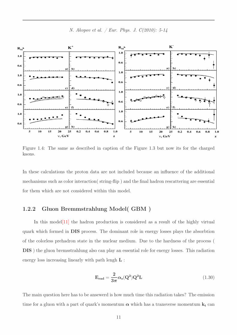
Figure 1.4: The same as described in caption of the Figure 1.3 but now its for the chargedkaons.
In these calculations the proton data are not included because an influence of the additional
mechanisms such as color interaction( string-flip ) and the final hadron rescattering are essential
for them which are not considered within this model.
1.2.2 Gluon Bremmstrahlung Model( GBM )
In this model[11] the hadron production is considered as a result of the highly virtual
quark which formed in DIS process. The dominant role in energy losses plays the absorbtion
of the colorless prehadron state in the nuclear medium. Due to the hardness of the process (
DIS ) the gluon bremsstrahlung also can play an essential role for energy losses. This radiation
energy loss increasing linearly with path lengh L :
Erad =2
3παs(Q
2)Q2L (1.30)
The main question here has to be ansewerd is how much time this radiation takes? The emission
time for a gluon with a part of quark’s momentum α which has a transverse momentum kt can
11

be estimated as :
tradiation ≈2ν
k2t
α(1−α) (1.31)
To form a leading hadron each radiated gluon can be considered as a quark-antiquark pair and
the fastes pair will produce a leading hadron later.
B.Z. Kopeliovich et al. / Nuclear Physics A 740 (2004) 211-245
Figure 1.5: The HERMES one dimensional data comparison with GBM model predictionsfor charged pions from nytrogen and krypton targets. The solid and dashed curves correspondto calculations with and without the effects of induced radiation, respectively.
When a time required for a quark to neutralize it’s colour ( production time ) is large,
the non-perturbative effects are dominated, hence to describe the hadronization process pertur-
batively one should consider fast hadrons i.e. hadrons with zh > 0.5. The produced colorless
object, the prehadron needs a time( formation time ) proportional to the hadron energy zhν
to form a final state hadron. If the leading hadron produced with fractional energy zh → 1
the gluon radiation is not allowed due to the energy conservation, leading to the Sudakov’s
suppression effect. The model predictions compared with the HERMES one dimensional
data are presented in the Figure 1.5.
12

1.2.3 Rescaling Models( RM )
In RMs ( also known as deconfined models ) the gluon radiation effect and the absorbtion
of produced hadrons taken into account[12]. In semi-inclusive DIS( SIDIS ) process, due to
the factorization, the cross section can be factorized into parton distribution functions( PDF )
and the quark fragmentation functions ( FF ). If a λ is the confinement scale then Q2 ∼ 1/λ2
and according to the deconfined models the λA confinement scale for nucleons inside a nucleus
should be greater than this for a free nucleon λ0.
λA > λ0 (1.32)
Since both PDF and FF are Q2 dependent, now due to the change of the confinement scale
A. Accardi et al. / Nuclear Physics A 720 (2003) 131-156
Figure 1.6: The HERMES multiplicity ratio for charged pions and kaons compared with therescaling model. The uper pair of curves includes rescaling without absorbtion for pisitivelyand negatively charged particles and the lower pair includes rescaling and also the nuclearabsorbtion by Bialas-Chmaj(BC) model.
13

this dependence should be rescalad as :
Q2 ≡ (λA
λ0
)2Q2 (1.33)
Taking into account also the Q2 dependence of QCD coupling constant the modification
can be done as :
qAf (x,Q
2) = qf (x, ξA(Q2)Q2) (1.34)
DAf (z,Q
2) = Df (z, ξA(Q2)Q2) (1.35)
With good approximation the DIS normalized hadron yeilds can be considered as a key to
touch on the fragmentation functions. In this sense the behavior of hadron multiplicity ratio
RhA can be interpreted as a consequence of such a modification. It is assumed that this approach
is available for the kinematic range z ≥ 0.1 and 0.1 < xBj < 0.6. In Figure 1.6 the comparison
of the model with the HERMES krypton data is provided.
1.2.4 BUU (Boltzmann-Uehling-Uhlenbeck) Transport Model
To describe the nuclear DIS process within the BUU model[13], the lepton-nucleuse
interaction considered in two steps. At first there is an interaction between high energetic
virtual photon with bounded nucleon inside a nucleus. This performed by the PYTHIA
and FRITIOF generators for two invariant mass ranges of the virtual photon-nucleon system :
W > 4 GeV and 2 < W < 4 GeV respectively. For a nucleon in a nuclear medium the possible
nuclear effects are also considered such as binding energy, Fermi motion and nuclear
shadowing. Then the coupled-chanel transport model used to describe the propogation of
a final state through the nuclear medium. The important thing has to be mentioned is the
different interpretations of the pre-hadron states in LUND and in transport models. This
difference caused by the production time concept in this two approaches. In the Lund model
it depends on the momentum of the string fragments while in the transport model the string
decays into color neutral pre-hadrons instantaneously. Therefore, here the hadron production
describes only with one scale, the formation time, when the interaction with nuclear medium
14

happens only by the beam and the target remnants. The formation time assumed to be a
constant in the hadron rest frame. During this time the pre-hadron interacts with surrounding
nuclear medium with a cross section which can be determined using the constituent quark
model.
σ∗
prebaryon =norg
3σbaryon, σ∗
meson =norg
2σmeson (1.36)
where norg is the number of (anti)quarks the pre-hadron consists which coming from beam or a
target. This means that for the vacuum created quark-antiquark pairs which formed a hadron
there is no interaction considered during the formation trime and those hadrons are move freely
in nuclear medium. Figure 1.7 shows the comparison of BUU model with the HERMES data
for pions, kaons and protons.
T. Falter et al. / Phys. Rev. C 70, 054609 (2004)
Figure 1.7: The HERMES multiplicity ratio from for different hadron species from kryp-ton(left) and neon(right) plots compared with BUU model simulations. The solid line repre-sents the results of simulation where the constituent quark concept for the prehadronic crosssection is used and a formation time is selected to be 0.5 fm/c. The dotted line on the left plotfor the proton spectrum indicates the result of simualtion for virtual photon-nucleon scatteringby PYTHIA and the dotted line on the right plot represents the result of a simualtion with apurely absorptive treatment of the final state interaction.
15

Chapter 2
The HERMES Experiment
The HERA measurement of spin (HERMES) data-taking program started in 1995 on
HERA acclereator at DESY in Hamburg. It was one of the four experiments on HERA
and had a goal to measure the spin structure of a nucleon. More than ten years of opera-
tion(the data-taking was stopped in 2007) it had acumulated a large variaty of data allowing
to investigate different aspects of the DIS process. The lepton ring used at HERMES stored
Figure 2.1: Schematic view of the HERA beam line with four experiments HER-MES,ZEUS,H1 and HERA B.
electrons or positrons at an energy of 27.6 GeV with typical beam current between 30-50
16

mA. In Figure 2.1 the scheme of the HERA accelerator is shown with four experimental halls.
2.1 The target system
The HERMES experiment uses a target[14] system with abilities to operate with pure
gaseous H, D, He, Ne, Kr, Xe in polorized(H,D) and unpolorized(H,D,He,Ne,Kr, Xe)
modes. It is internal to the beam line(see Figure 2.2) with 40 cm long storage cell which is
cooling up to 70 K and has an elliptical cross section of 9.8 x 24 mm2. To provide as much
areal density as possible the gas injected to the storage cell aligned collinear to the beam line.
Figure 2.2: The HERMES target system.
This allowes to get a target density up to ∼ 1016 nucleons per cm2 for polorized hydrogen and
deuterium targets.
2.2 The HERMES spectrometer
The HERMES spectrometer[15] is the forward angle spectrometer with angular accep-
tance of ±( 40 - 140 ) mrad in vertical and ± 170 mrad in horizontal directions(see Figure
2.3). The HERMES coordinate system has a z axis along the beam lepton momentum with
coordinate zero in the center of target cell. The xy axis construct in such a way that y pionts to
the up direction and x points to the left when looking to the downstream of the beam pipe. The
spectrometer consists of two detector subsystems : the tracking system which provides particle
17

track reconstruction and the particle identification( PID ) system : to separate leptons from
hadrons and ability to identify between different hadron flavors.
Figure 2.3: The HERMES spectrometer(tracking detectors in red and PID detectors in green).
2.2.1 The Spectrometer Magnet
The HERMES spectrometer has a dipole magnet with integrated deflecting power equal
to 1.3 Tm. To avoid from possible influence of the spectrometer magnet on the HERA beam,
the beam pipe is shielded by 11 cm thick septum steel plate which limits the lower vertical
acceptance of the spectrometer to ±40 mrad. On the other hand the spectrometer magnet
limits the upper acceptance in the vertical direction in ±( 140 ) mrad window.
2.2.2 Tracking Detectors
In order to reconstruct a particle track the tracking chambers are used which are placed
in front of the magent inside the magnet and behind the magnet. They are the wirechambers
except the silicon detector which is installed right after the target. The goal of the tracking
system is to provide a determination of the origin, angles and momentum of charged particle
tracks.
18

The Silicon Detector
To increase the acceptance for long-living particles such as Λ,Λc,Ks the silicon detec-
tor[16] was installed. In this analisys the data from this detector is not used.
The Drift Vertex Chambers (DVC)
The goal of DVC chambers was to improve the momentum resolution. They have a 200
µm spatial resolution with 2 mm wire spacing.
The Front Chambers (FC)
The front chambers[17] were used to reconstruct the front tracks. They filled with a gas
mixture Ar/CO/CH4 and consist of two modules with 7 mm width and 8 mm depth. The
spatial resolution provided by these chambers is 225 µm and the efficiencies are varied between
97− 99% depending on the position in the cell.
The Magnet Chambers (MC)
The magnet chambers[18] were installed inside the spectrometer magnet gap. There were
three sets of wire chambers allowing to reconstruct a momentum of low energy particles which
have been not reached to the back part of the spectrometer.
The Back Chambers (BC)
In order to reconstruct a particle tracks behind the spectrometer magnet the two sets
of back chambers[19] were installed in front of and behind the Ring-Imaging Čerenkov
detector. They had the spatial resolution 210 µm for the first set(BC1/2) and 250 µm for
the second set(BC3/4). The efficiency for the lepton track is about 99% while for hadron
track it is a bit lower : 97% which caused by the lower ionization for hadrons compared with
the leptons.
In Figure 2.4 a schematic view for short and long tracks reconstructed by the HERMES tracking
system is shown.
19

Figure 2.4: A long(in red) and short(in black) track reconstruction by the HERMES trackingsystem.
2.2.3 Particle Identification (PID)
The aim of the HERMES particle identification system is to identify the tracks recon-
structed by the tracking system. In this sense the first thing to do is to distinguish a lepton
track from a hadron track. The idea is to use different detectors taking into account the fact
that a lepton(either electron or positron) and a hadron will have a different energy deposites in
these detectors thus one can separate between lepton and hadron tracks combining the results
from different detectors with the unified algorithm called as PID algorithm.
The Transition Radiation Detector (TRD)
When the particles travers the boundary of two different media with different dielectric
indices the transition radiation emits and the intensity of this radiation depends on the Lorentz
factor ( γ = E/mc2 ). The usage of a multilayer radiator TRD allowes to use the threshold
condition to distinguish between different particles. The electron/positrons exceed threshold
which is around γ ∼ 1000 at energies greater than 0.5 GeV while for the lightest hadron : the
pion this limit is around 140 GeV due to about two order mass differences between them.
The HERMES Transition Radiation Detector consists by six identical layers each of
which constructed with a fiber radiator and a wire chamber. Each track being either lepton
or hadron has an energy deposition in wire chamber and with combination of the transition
radiation it turns out that the energy deposit for leptons is twice larger than for the hadrons.
20

The Calorimeter
The HERMES has a lead glass electromagnetic calorimeter consisted of 420 radi-
ation blocks[20]. The particles deposit their energy in the calorimeter making electromagnetic
showers which for leptons caused the loss of the almost all their energy. This means that the
energy deposit to momentum ratio for leptons will be very close to unity while for hadrons this
value is about two times smaller.
On the other hand the calorimeter allowes to reconstruct electroneutral particles such as
π0 and η mesons registerating a decay components: the photons. It is also used as a fast
first-level trigger for scattered beam leptons.
The Preshower Detector
The HERMES hodoscope system which used for the triggering consists of three ho-
doscopes : H0, H1 and H2 where H2: the preshower provides also the PID information. It
has 11 mm lead between 1.3 mm stainless steel sheets which leads a very small energy deposi-
tion for hadrons at the level of few MeV while for leptons the energy deposition in magnitude
is one order higher.
2.2.4 The RICH Detector
The HERMES RICH detector[21] provides the identification of charged hadrons such
as pions, kaons, protons and antiprotons in momentum range : 2 GeV < ph < 15 GeV. It
uses the Čerenkov radiation effect i.e. the radiation of a relativistic, charged particles moving
through the medium with velocities greater than the velocity of the speed in the same medium:
v > c/n (2.1)
where n is the refractive index of the medium and c is the speed of light. The angle of Čerenkov
radiation depends on a particle velocity and the medium refractive index and can be written
as :
cosθ = c/nv (2.2)
21

0
0.05
0.1
0.15
0.2
0.25
0 2 4 6 8 10 12 14 16 18 20p [GeV]
Θ C [r
ad]
π
K
p
Figure 2.5: Momentum dependence of the Čerenkov angle for different hadron types and ra-diators. The upper band corresponds to the aerogel and the lower band to the C4F10 gasrespectively.
Thus particles with the same momentum will have a different radiation angles depending on
their masses( or types ).
Two radiators are used in the HERMES RICH detector. A silica aerogel with re-
fractive index 1.0304 and a C4F10 gas which has the refractive index equal to 1.00137. The
combination of these two radiators allows to separate between pions, kaons and protons as it
is shown in Figure 2.5.
2.2.5 The PID Algorithm
Using the signal information from the particle identification detectors the PID al-
gorithm used to manipulate with tracks to make the identity for them. The HERMES PID
algorithm based on the Bayes theorem which can be read as :
P(x | y) =P(y | x)P(x)
P(y)(2.3)
22

where P(x | y) is the probability for x to be an y and P(x)(P(y)) is the overall probability
for x(y). Thus the PID value can be defined as :
PID = P(Tl(h) | R,k) (2.4)
where P(Tl(h) | R,k) is the probability that the track with parameter k(p, θ)( the k parameter
describes a track with momentum p and the polar angle θ ) lepton( hadron ) having a detector
response R. Using the Bayes theorem one can get :
P(Tl(h) | R,k) =P(R | Tl(h),p)P(Tl(h) | k)
P(R | k)(2.5)
Here P(R | k) is the probability for a track with parameter k to have a response R in a detector.
It can be presented as :
P(R | k) = P(R | Tl,h,k)P(Tl,h,k) (2.6)
which is summed over all lepton( hadron ) tracks with parameter k. In equation (2.6) the first
component of this product is the overall probability named as the parent distributions which is
detector dependent and the P(Tl,h,k) represents the flux of leptons( hadrons ) which depends
on track atributes : the parameter k. Eventually the PID value for lepton-hadron separation
can be defined in following way :
PID = log10
P(Tl | R,k)
P(Th | R,k)(2.7)
where the logarithm is used just for a technical reason to provide a PID sign difference be-
tween leptons and hadrons. Using the equations (2.5) and (2.6) this logarithmic ratio can be
transformed as :
PID = PIDDetector − log10(Flux) (2.8)
where PIDDetector is the ratio of detector dependent parent distributions and the Flux and
can be written as :
Flux ≡P(Tl | k)
P(Th | k)(2.9)
23

In Figure 2.6 the PID distribution is presented which clearly shows the separation of hadrons
PID-50 -40 -30 -20 -10 0 10 20 30 40 500
500
1000
1500
2000
310×
Figure 2.6: The PID distribution for DIS event sample from the HERMES data.
from leptons at PID value equal to zero. The HERMES PID provides a very efficient
separation with less than one percent contamination of leptons with hadrons.
2.2.6 The HERMES Luminosity Measurement
The HERMES luminosity measurement is based on the measurement of the elastic
Möller and Bhabha scattering for electron and positron respectively. When the beam is a
positron, apart from Bhabha scattering also an anihillation takes place. The reaction products
are detecting by two calorimeters installed at the left and right sides of the beam pipe.
The Möller and Bhabha scattering processes and the electron-positron anihillation
is calculable within quantum electrodynamics( QED ). To have the luminosity of the experi-
ment the measured rate of the luminosity monitors( calorimeters ) is divided on QED calculated
cross sections of Möller and Bhabha processes[22].
2.3 Data Analysis
For this analysis we have used data from DIS/SIDIS processes on D, Ne, Kr, Xe
targets using either electron or positron beams. The HERMES provides a large data set
24
for charged separated hadrons in DIS regime which allowed us to make a multidimensional
view of the effect of our interest : the nuclear attenuation effect.
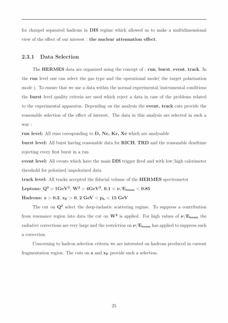
2.3.1 Data Selection
The HERMES data are organized using the concept of : run, burst, event, track. In
the run level one can select the gas type and the operational mode( the target polarization
mode ). To ensure that we use a data within the normal experimental/instrumental conditions
the burst level quality criteria are used which reject a data in case of the problems related
to the experimental apparatus. Depending on the analysis the event, track cuts provide the
reasonable selection of the effect of interest. The data in this analysis are selected in such a
way :
run level: All runs coresponding to D, Ne, Kr, Xe which are analysable
burst level: All burst having reasonable data for RICH, TRD and the reasonable deadtime
rejecting every first burst in a run
event level: All events which have the main DIS trigger fired and with low/high calorimeter
threshold for polorized/unpolorized data
track level: All tracks accepted the fiducial volume of the HERMES spectrometer
Leptons: Q2 > 1GeV2, W2 > 4GeV2, 0.1 < ν/Ebeam < 0.85
Hadrons: z > 0.2, xF > 0, 2 GeV < ph < 15 GeV
The cut on Q2 select the deep-inelastic scattering regime. To suppress a contribution
from resonance region into data the cut on W2 is applied. For high values of ν/Ebeam the
radiative corrections are very large and the restriction on ν/Ebeam has applied to suppress such
a correction.
Concerning to hadron selection criteria we are interested on hadrons produced in current
fragmentation region. The cuts on z and xF provide such a selection.
25

2.4 The RICH Unfolding
The hadron identification is one of the main topics of this analysis. It performs by RICH
which uses the spherical mirrors to reflect the Čerenkov radiation into the photon detector
which is an array of photomultiplier tubes placed above the mirror( Figure 2.7 ). Knowing the
track momentum from the tracking system and measuring it’s velocity using the opening angle
of the Čherenkov photons one can reconstruct a particle type by reconstructing it’s mass. The
Figure 2.7: Particle identification by the RICH detector.
problems begin when the two tracks are very close to each other. In this case the overlaping
of the photon rings can be the cause for the track misidentification. This issue is dominated
in case of the electron track combined with any of the hadron track especially with the proton
track. Assume the electron track satisfy the threshold conditions for the Čherenkov radiation in
both radiators and the proton track which is very close to it, does not( Figure 2.8 b ). Using the
information from the tracking system the proton track can be misidentified as a kaon using the
fake identity of lepton ring with kaon one. The another possiblity is low momentum particles
mainly the protons bended at the edges of the detector and that is why misidentifyded, using
lepton rings pattern, into kaons( Figure 2.8 a ). In order to avoid from such an effect there
is a necessity to tune the RICH parameters such as the yields of Čherenkov photons and the
distribution of the Čherenkov angles. There are two ways to do this, first use the experimental
data sample to reconstruct the decaying particles with known invariant masses and the second
method is the usage of the Monte Carlo simulation. The first way has problems concerning
26

x x
e aerogel ring
e C4F10 ring
e hit p hit
a. b.
reconstructedK aerogel ring
x
e aerogel ring
e C4F10 ring
e hit
reconstructedK aerogel ring
xp hit
Figure 2.8: Particle misidentification in the RICH detector.
to statistics which is very important in studies of topologies for different kinematical regiems.
Hence the RICH Monte Carlo simualtion is used to construct the so-called P martrices which
are the statistical weights for given track to be a pion, kaon or a proton. The goal of the RICH
unfolding to reweight the identity of tracks using these weigths. Since the effective performance
of RICH detector depends on track momentum and the event topology( how many tracks there
are in detector half ). Having this information from data sample one can unfold the identified
hadrons to get the true ones using the equation (2.10) :
Iπ
IK
Ip
IX
=
P ππ PK
π P pπ PX
π
P πK PK
K P pK PX
K
P πp PK
p P pp PX
p
Tπ
TK
Tp
TX
(2.10)
In this equation Ii represents the identified/nonidentified hadrons( π, K, p and X is noniden-
tified hadron tracks ) and Ti’s are the true hadron type after the unfolding. The values for
Pj
i are the probability that the true type hadron i will be identify as a type j. To get the
final true hadron type distributions one should solve this matrix equation just inverting the P
matrix. To do this we should truncated the P matrix( make it the square matrix eliminating
the column for non identified probabilities ) assuming that the contamination of nonidentified
tracks is very small which is the case for the HERMES RICH detector.
~T = P−1~I (2.11)
27

A momentum dependence of non-unfolded( raw ) and RICH unfolded hadron yields is shown
in Figure 2.9. We can see the clear indication of the RICH radiator transition between 8 - 11
GeV region. The large discrepancies between raw and unfolded data at low momentum region
caused by the RICH identification problems for those tracks due to the large bending which
leads the tracks to hit the edges of the detector where the registration efficiencies are relatively
small.
Momentum-15 -10 -5 0 5 10 15
Yie
ld
0
20000
40000
πRawUnfolded
negative
charge
positive
charge
Momentum-15 -10 -5 0 5 10 15
Yie
ld
0
5000
10000KTop Half
negative
charge
positive
charge
Momentum-15 -10 -5 0 5 10 15
Yie
ld
0
5000
10000
15000 proton
negative
charge
positive
charge
Momentum-15 -10 -5 0 5 10 15
Yie
ld
0
20000
40000
Momentum-15 -10 -5 0 5 10 15
Yie
ld
0
5000
10000
Bottom Half
Momentum-15 -10 -5 0 5 10 15
Yie
ld
0
5000
10000
15000
Figure 2.9: The influence of RICH unfolding on charged hadron yields. In red a raw datais shown without correction for RICH on misidentification effects. Blue points are alreadycorrected for RICH misidentification effects. The comparison is done for both detector halvesseparately. There is a clear indication of the RICH radiator transition between 8 - 11 GeVmomentum range.
2.5 Charged Hadron Yields
The study of hadron yields plays an important role in hadron physics. It’s because one
can use the hadron yields to make the hadron multiplicity ( i.e. the hadron yields normalized
on DIS leptons ) which carries an important information about the fragmentaion process. This
quantity( 2.12 ) depends on several kinematical variables such as the virtual photon energy ν,
the hadron fractional energy z, the momentum component of hadron transverse to the virtual
28

photon direction pt which are studed in this analysis. It depends also on the photon virtuality
Q2 and the azimuthal angle ϕ which is an angle between lepton scattering and the hadron
production planes. The last two dependencies are almost vanished in "super ratio" which is
used to study the nuclear attenuation effect. Hence the main concentration was done on ν, z
and pt distributions.
M =Nh(ν,Q2, z,pt,ϕ)
Ne(ν,Q2)(2.12)
The z disribution of charged hadron yields is shown in Figure 2.10. Similarily to momentum
distribution the identification problems reveals at very low z range, a part of which is cut-off
using the data selection criterium to select the current fragmentation region : z > 0.2. Apart
z0 0.2 0.4 0.6 0.8 1
Yie
ld
0
50
100
150
310×
+πRawUnfolded
z0 0.2 0.4 0.6 0.8 1
Yie
ld
0
5000
10000
15000
+K
z0 0.2 0.4 0.6 0.8 1
Yie
ld
0
10000
20000
30000proton
z0 0.2 0.4 0.6 0.8 1
Yie
ld
0
50
100
150
310×-π
z0 0.2 0.4 0.6 0.8 1
Yie
ld
0
5000
10000
15000 -K
z0 0.2 0.4 0.6 0.8 1
Yie
ld
0
2000
4000
6000
8000antiproton
Figure 2.10: The z dependence of charged hadron multiplicities. The misidentification effect islarger at small z values, particularly for protons and antiprotons.
from cut on the z the xF > 0 cut is used to select hadrons from current fragmentation region.
The corresponding hadron yields with cut on xF are presented in Figure 2.11. Here one can
see the huge flux change for protons and antiprotons at small z values while for kaons it is
relatively small and there is practically no changes for pions. The impact of hadronic cuts on
charged hadron yields is shown in Figure 2.12. One can see that the cut on z is already satisfied
29

z0 0.2 0.4 0.6 0.8 1
Yie
ld
0
50
100
150
310×
+πRawUnfolded
> 0Fx
z0 0.2 0.4 0.6 0.8 1
Yie
ld
0
5000
10000
15000
+K
z0 0.2 0.4 0.6 0.8 1
Yie
ld
0
10000
20000
30000proton
z0 0.2 0.4 0.6 0.8 1
Yie
ld
0
50
100
150
310×-π
z0 0.2 0.4 0.6 0.8 1
Yie
ld
0
5000
10000
15000 -K
z0 0.2 0.4 0.6 0.8 1
Yie
ld
0
2000
4000
6000
8000antiproton
Figure 2.11: The z dependence of charged hadron multiplicities with cut on xF. The Feynmanvariable cuts more protons and antiprotons coming from the target fragmentation region.
p GeV2 4 6 8 10 12 14 16
Yie
ld
0
50
100
150
310×
+πAllz > 0.2
> 0F
z > 0.2, x
p GeV2 4 6 8 10 12 14 16
Yie
ld
0
5000
10000
15000
20000+K
p GeV2 4 6 8 10 12 14 16
Yie
ld
0
20000
40000
proton
p GeV2 4 6 8 10 12 14 16
Yie
ld
0
50
100
150
310×-π
p GeV2 4 6 8 10 12 14 16
Yie
ld
0
5000
10000-K
p GeV2 4 6 8 10 12 14 16
Yie
ld
0
5000
10000
15000antiproton
Figure 2.12: The impact of hadronic cuts on raw hadron momentum dependent yields.
30

to xF > 0 condition for pions and also for kaons while for protons and antiprotons there is a
large contribution from target fragmentation region at small momentum range.
The ν dependence of charged hadron multiplicities is shown in Figure 2.15. We can
see that the main hadron statistics is populated in the ν range 10 - 12 GeV. The usage of
standard DIS cuts Q2 > 1GeV2,W2 > 4GeV2 restrict the lower limit of ν to be greater than
∼ 2.2 GeV. The upper limit for ν is given with a cut on y = νEbeam
< 0.85 which leads to the
restriction ν < 23.5 GeV. It is also seen that the huge amount of negatively charged kaons are
misidentified as antiprotons.
In Figure 2.16 the transverse momentum dependence of charged hadrons multpliciteis is
shown. The HERMES allowes to reach the transverse momentum range up to 1.5 - 1.7 GeV.
Beyond to the collinear case the pt studies of the hadron multiplicities play an important role
for nucleon three dimensional structue investigations. The point here to study, how the intrisic
transverse momentum of parton generates the final hadron transverse momentum component
which provide a much deeper understanding of QCD and hadron structure. In contrast to the
collinear factorization, here the integration over the parton transverse momentum is left which
leads to the more general transverse momentum dependent(TMD) factorization.
As it was already mentioned, using the hadron multiplicities one can access to the frag-
mentation functions which are assumed to be independent of xBj but only depend on z. On the
other hand these transverse momentum dependent fragmentation functions are not yet fully
understood. This is a relatively new task to study and this subject called the transversity.
There are several approaches to describe the transverse momentum dependent fragmentation
functions[23][24]. The commonly known method is the Gaussian parametrization or the so-
called Gaussian anzats[25]. The fragmentation functions in this approach have a form[26] :
DH/f (z,KT) = dH/f ·exp[−K2
T/ < K2T >]
π < K2T >
(2.13)
where KT is the hadron transverse momentum in the photon rest frame. Therefore the
pt distribution for charged hadron multiplicities is very importanat to test different hypothesis
existing at the moment.
In Figure 2.17 one can see the correlation between different kinematical variables for
31

GeVν0 5 10 15 20 25
Yie
ld
0
20000
40000
60000
80000+πRaw
Unfolded
GeVν0 5 10 15 20 25
Yie
ld
0
5000
10000+K
GeVν0 5 10 15 20 25
Yie
ld
0
5000
10000
15000 proton
GeVν0 5 10 15 20 25
Yie
ld
0
20000
40000
60000
80000-π
GeVν0 5 10 15 20 25
Yie
ld
0
2000
4000
6000 -K
GeVν0 5 10 15 20 25
Yie
ld
0
1000
2000
3000
4000 antiproton
Figure 2.13: The ν dependence of charged hadron multiplicities. The RICH misidentificationeffect is spread over whole range of ν.
GeVt
p0 0.5 1 1.5
Yie
ld
210
310
410
510 +π
RawUnfolded
GeVt
p0 0.5 1 1.5
Yie
ld
210
310
410
+K
GeVt
p0 0.5 1 1.5
Yie
ld
210
310
410proton
GeVt
p0 0.5 1 1.5
Yie
ld
210
310
410
510 -π
GeVt
p0 0.5 1 1.5
Yie
ld
210
310
410-K
GeVt
p0 0.5 1 1.5
Yie
ld
210
310
410 antiproton
Figure 2.14: The pt dependence of charged hadron multiplicities. The RICH misidentificationeffect is dominated at small pt range.
32
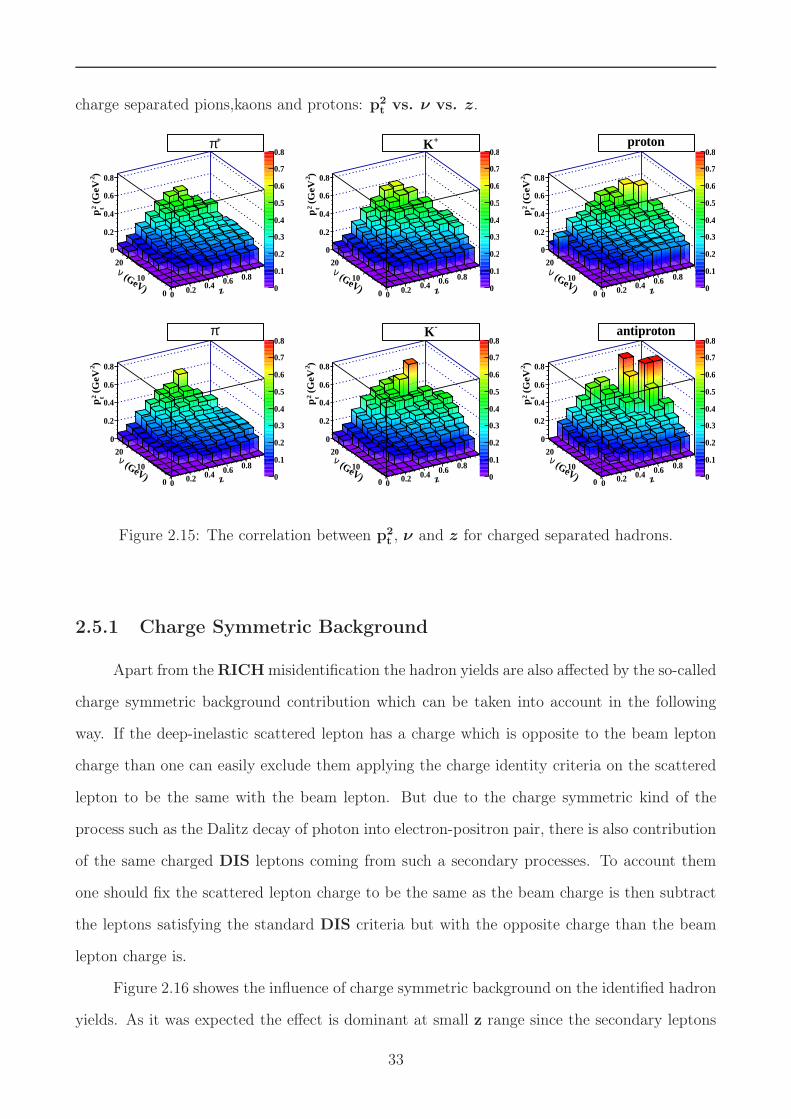
charge separated pions,kaons and protons: p2t vs. ν vs. z.
z0 0.2 0.4 0.6 0.8 1 (GeV)
ν
0
10
20
)2 (
Ge
V2 t
p
0
0.2
0.4
0.6
0.8
0
0.1
0.2
0.3
0.4
0.5
0.6
0.7
0.8+π
z0 0.2 0.4 0.6 0.8 1 (GeV)
ν
0
10
20
)2 (
Ge
V2 t
p
0
0.2
0.4
0.6
0.8
0
0.1
0.2
0.3
0.4
0.5
0.6
0.7
0.8+K
z0 0.2 0.4 0.6 0.8 1 (GeV)
ν
0
10
20
)2 (
Ge
V2 t
p
0
0.2
0.4
0.6
0.8
0
0.1
0.2
0.3
0.4
0.5
0.6
0.7
0.8proton
z0 0.2 0.4 0.6 0.8 1 (GeV)
ν
0
10
20
)2 (
Ge
V2 t
p
0
0.2
0.4
0.6
0.8
0
0.1
0.2
0.3
0.4
0.5
0.6
0.7
0.8
-π
z0 0.2 0.4 0.6 0.8 1 (GeV)
ν
0
10
20
)2 (
Ge
V2 t
p
0
0.2
0.4
0.6
0.8
0
0.1
0.2
0.3
0.4
0.5
0.6
0.7
0.8
-K
z0 0.2 0.4 0.6 0.8 1 (GeV)
ν
0
10
20
)2 (
Ge
V2 t
p
0
0.2
0.4
0.6
0.8
0
0.1
0.2
0.3
0.4
0.5
0.6
0.7
0.8antiproton
Figure 2.15: The correlation between p2t , ν and z for charged separated hadrons.
2.5.1 Charge Symmetric Background
Apart from the RICH misidentification the hadron yields are also affected by the so-called
charge symmetric background contribution which can be taken into account in the following
way. If the deep-inelastic scattered lepton has a charge which is opposite to the beam lepton
charge than one can easily exclude them applying the charge identity criteria on the scattered
lepton to be the same with the beam lepton. But due to the charge symmetric kind of the
process such as the Dalitz decay of photon into electron-positron pair, there is also contribution
of the same charged DIS leptons coming from such a secondary processes. To account them
one should fix the scattered lepton charge to be the same as the beam charge is then subtract
the leptons satisfying the standard DIS criteria but with the opposite charge than the beam
lepton charge is.
Figure 2.16 showes the influence of charge symmetric background on the identified hadron
yields. As it was expected the effect is dominant at small z range since the secondary leptons
33

z0 0.2 0.4 0.6 0.8 1 1.2
(cs
b)
+π
0.92
0.94
0.96
0.98
1
1.02
z0 0.2 0.4 0.6 0.8 1 1.2
(cs
b)
+K
0.92
0.94
0.96
0.98
1
1.02
z0 0.2 0.4 0.6 0.8 1 1.2
pro
ton
(cs
b)
0.92
0.94
0.96
0.98
1
1.02
z0 0.2 0.4 0.6 0.8 1 1.2
(cs
b)
-π
0.92
0.94
0.96
0.98
1
1.02
z0 0.2 0.4 0.6 0.8 1 1.2
(cs
b)
-K
0.92
0.94
0.96
0.98
1
1.02
z0 0.2 0.4 0.6 0.8 1 1.2
antip
roto
n (
csb)
0.92
0.94
0.96
0.98
1
1.02
Figure 2.16: Charged symmetric background effect on charged hadron yields. The effect isessential at small z values. It is less than 2% for the data of interest : z > 0.2.
produced by the Dalitz decay supposed to have a low momenta. The maximum effect in the
range of interest ( z > 0.2 ) is estimated less than 2%.
2.6 The HERMES Monte Carlo Package
The aim of the HERMES Monte Carlo is to generate a DIS process and propagate a
physical event through the simulated spectrometer. This is an important tool to understand
the experimental data and to estimate the various effects coming from detector resolutions and
the spectrometer acceptance. To do this a physical event is generated in kinematical bins of ν
and Q2 according to the corresponding cross section d2σdνQ2 . The scattering process required the
knowledge of the parton distribution functions (PDFs). There are several parametrizations
based on the experimental data : GRV[27], MRS[28]. The commonly used one is provided
by CTEQ6[29] collaboration. The next step is to introduce a hadronization which can be
done only by phenomenological approach. The HERMES Monte Carlo uses the JETSET
package which based on the LUND[8] model.
The HERMES Monte Carlo is a chain of different programs which together make
34
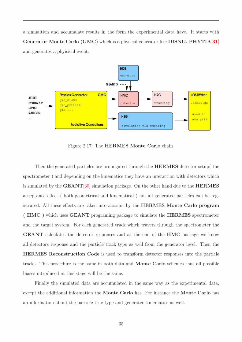
a simualtion and accumalate results in the form the experimental data have. It starts with
Generator Monte Carlo (GMC) which is a physical generator like DISNG, PHYTIA[31]
and generates a phyisical event.
Figure 2.17: The HERMES Monte Carlo chain.
Then the generated particles are propogated through the HERMES detector setup( the
spectrometer ) and depending on the kinematics they have an interaction with detectors which
is simulated by the GEANT[30] simulation package. On the other hand due to the HERMES
acceptance effect ( both geometrical and kinematical ) not all generated particles can be reg-
istrated. All these effects are taken into account by the HERMES Monte Carlo program
( HMC ) which uses GEANT programing package to simulate the HERMES spectrometer
and the target system. For each generated track which travers through the spectrometer the
GEANT calculates the detector responses and at the end of the HMC package we know
all detectors response and the particle track type as well from the generator level. Then the
HERMES Reconstruction Code is used to transform detector responses into the particle
tracks. This procedure is the same in both data and Monte Carlo schemes thus all possible
biases introduced at this stage will be the same.
Finally the simulated data are accumulated in the same way as the experimental data,
except the additional information the Monte Carlo has. For instance the Monte Carlo has
an information about the particle true type and generated kinematics as well.
35

2.6.1 Event Generators
The HERMES generator Monte Carlo program( GMC ) uses two steps for the event
generation. In the first step a physics generator simulates the interaction of the initial state
particles. Then in the next step the hadronisation take place evolving the initial system into
the final state using JETSET program, based on the LUND string fragmentation model.
In GMC level the commonly used package is the DISNG package which generats a deep-
inelastic scattering process. It uses two generators for poloraized and unpolorized cases : the
PEPSI[32] and the LEPTO[33] respectively. Despite LEPTO and PEPSI are an excellent
tool to study the DIS process, the number of physics processes which they consider is limited.
In particular, they do not account for the exclusive production of vector mesons due to the
complication of the particle production process at z → 1 in the LUND model. For this cases
one can use the PYTHIA event generator which can generate a large variaty of the physical
processes.
z0 0.2 0.4 0.6 0.8 1 1.2
mul
t.
0
0.005
0.01
0.015
0.02
0.025
+πRaw
RICH Unfolded
MC DISNG
z0 0.2 0.4 0.6 0.8 1 1.2
mul
t.
0
0.001
0.002
0.003 +K
z0 0.2 0.4 0.6 0.8 1 1.2
mul
t.
0
0.002
0.004
0.006
0.008
proton
z0 0.2 0.4 0.6 0.8 1 1.2
mul
t.
0
0.005
0.01
0.015
0.02
-π
z0 0.2 0.4 0.6 0.8 1 1.2
mul
t.
0
0.0005
0.001
0.0015
0.002-K
z0 0.2 0.4 0.6 0.8 1 1.2
mul
t.
0
0.0002
0.0004
0.0006
0.0008
0.001
0.0012
antiproton
Figure 2.18: Data Monte Carlo comparision for charged hadron multiplicities. In green themultiplicity data from DISNG Monte Carlo is shown in comparison with experimental datawith(blue) and without(red) correction for the RICH misidentification effect.
36

2.6.2 Unfolding for Radiative Effects and Detector Smearing
Due to the fact that the detectors have a certain resolution and the beam lepton can
radiate a real photon(initial state radiation ISR) or the same can happen with the scattered
lepton(final state radiation FSR) the true kinematics can be changed(see Fig. 2.19). In order
to correct for such effects the DISNG Monte Carlo is used. The idea is to compare the re-
Figure 2.19: True kinematic change due to the radiative effects.
constructed kinematics which includes these effects with a generated ones making a correction
matricies named as the smearing matricies. For this purpose, bin-by-bin migration of events
due to the kinematic change is calculated in terms of migration matrix elements and the ex-
perimental data ara corrected using these elements. Technically it can be calculated in such a
way[34]. We use two Monte Carlo samples. The first one includes the experimental setup and
possible radiative effects. Here we have fully tracked Monte Carlo production which should be
used for calculation of elements of the migrartion matricies. The idea is to fix kinematical bin
in experimental level and look to which Born bin i.e. the bin with corresponding true kine-
matics it corresponds to. If one make a numeration than one should consider two indices i for
experimental Monte Carlo sample and j for Born or generator level sample. In this way one get
a matix, each element of which has an information about real event migration due to the true
37
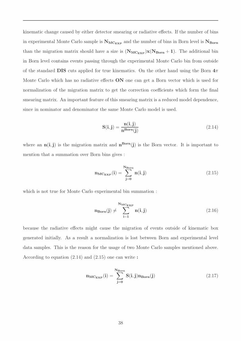
kinematic change caused by either detector smearing or radiative effects. If the number of bins
in experimental Monte Carlo sample is NMCEXPand the number of bins in Born level is NBorn
than the migration matrix should have a size is (NMCEXP)x(NBorn + 1). The additional bin
in Born level contains events passing through the experimental Monte Carlo bin from outside
of the standard DIS cuts applied for true kinematics. On the other hand using the Born 4π
Monte Carlo which has no radiative effects ON one can get a Born vector which is used for
normalization of the migration matrix to get the correction coefficients which form the final
smearing matrix. An important feature of this smearing matrix is a reduced model dependence,
since in nominator and denominator the same Monte Carlo model is used.
S(i, j) =n(i, j)
nBorn(j)(2.14)
where an n(i, j) is the migration matrix and nBorn(j) is the Born vector. It is important to
mention that a summation over Born bins gives :
nMCEXP(i) =
NBorn∑
j=0
n(i, j) (2.15)
which is not true for Monte Carlo experimental bin summation :
nBorn(j) 6=
NMCEXP∑
i=1
n(i, j) (2.16)
because the radiative effects might cause the migration of events outside of kinematic box
generated initially. As a result a normalization is lost between Born and experimental level
data samples. This is the reason for the usage of two Monte Carlo samples mentioned above.
According to equation (2.14) and (2.15) one can write :
nMCEXP(i) =
NBorn∑
j=0
S(i, j)nBorn(j) (2.17)
38

Coming to the real experimental sample one can write the experimental distribution following
to the Monte Carlo simulation in such a way :
Exp(i) = Lumi ·Eff(i) ·
NBorn∑
j=0
S(i, j)nBorn(j) (2.18)
where the Lumi is the overall luminosity of process and Eff(i) is a factor which includes the
detector efficiencies. In case of multiplicity ratio this two factors are taking off and the final
equation for smearing and radiative effects looks like :
Born(j) =1
σBorn
·
NMCEXP
∑
i=1
S−1h (j, i)
(
Exp(i) · σMCTrk−Background(i, 0)
)
(2.19)
Here the S−1h (j, i) is a truncuated inversed smearing matrix, σBorn is the inclusive cross sections
from Born Monte Carlo and σMCTrkis the inclusive cross sections from tracked Monte Carlo.
It is important to mention that by Born(j) and Exp(i) one should assume the multiplicity
ratio in 4π and in acceptance respectively.
Due to the complications related to Monte Carlo simulations for heavy nuclear targets
and taking into account the fact that we are interested in the nuclear attenuation effect which
is multiplicity super ratio, we assume that these effects are mainly cancel out, that is why we
don’t use 4π unfolding technik in this analysis.
39

Chapter 3
Results and Conclusions
The data from semi-inclusive deep-inelastic scattering process off different nuclear targets
are analysed. The hadron DIS normalized yileds( the multiplicities ) are extracted. They are
corrected for the RICH detector possible misidentification effects. Using the hadron multiplic-
ity ratios RhA the nuclear attenuation effect is studied in two dimensional[35] manner. For all
data plots the scale uncertainties are estimated to be 3%, 5%, 4%, and 10% for pions, kaons,
protons and antiprotons, respectively. The results of RhA are presented for neon (Ne),
krypton (Kr) and xenon (Xe) targets for charge separated pions, kaons and protons us-
ing a fine binning in one of the kinematical variables and three slices in a second variable.
This allows to study the effect of interest in more detailes, suppressing the correlations between
different kinematical variables. The large statistics and the accurate measurement provided by
the HERMES spectrometer allowes us to have the first multidimensional data for the nuclear
attenuation effect in a wide kinematic range.
3.1 ν dependence in three z slices
In Figure 3.1, the ν dependence of RhA is shown in three z slices. The global feature for the
multiplicity ratio is the decreasement with increasing of target atomic mass A which can be
qualitatively understood in sense of the strengthening of energy loss proccesses due to the
enhancment of the nuclear matter density.
With the increasing of ν an enhancement of RhA was observed for pions(π+, π−) and
40

0.2
0.4
0.6
0.8
1
1.2
10 20
0.2
0.4
0.6
0.8
1
1.2
10 20
0.2
0.4
0.6
0.8
1
1.2
10 20
0.5
1
1.5
10 20
0.5
1
1.5
10 20
0.5
1
1.5
10 20
0.5
1
1.5
10 20
0.5
1
1.5
10 20
z = 0.2-0.4z = 0.4-0.7z > 0.7
0.4
0.6
1.0
0.8
RAh
Ne Kr
π+
Xe
0.5
1.0
1.5
K+
0.5
1.0
1.5
10 20 10 20 2010
p
ν [GeV]
0.5
1
1.5
10 20
0.2
0.4
0.6
0.8
1
1.2
10 20
0.2
0.4
0.6
0.8
1
1.2
10 20
0.2
0.4
0.6
0.8
1
1.2
10 20
0.5
1
1.5
10 20
0.5
1
1.5
10 20
0.5
1
1.5
10 20
0.5
1
1.5
10 20
0.5
1
1.5
10 20
z = 0.2-0.4z = 0.4-0.7z > 0.7
0.4
0.6
1.0
0.8
RAh
Ne Kr
π-
Xe
0.5
1.0
1.5
K -
0.5
1.0
1.5
10 20 10 20 2010
p–
ν [GeV]
0.5
1
1.5
10 20
Figure 3.1: Dependence of RhA on ν for three slices in z. There is an enhancment of the nuclear
attenuation effect with increasing of the nuclear target mass. For protons we see a differentbehaviour than for mesons and antiprotons.
negatively charged kaons(K−) which is consistent with fragmentation models, explaining such a
behaviour as a result of Lorentz dilation and/or a modification of the fragmentation function[36].
This kind of behaviour was observed in EMC collaboration[4] and later by the HERMES one
dimensional data[5] but in contrast to the negatively charged kaons (K−), the ν dependence of
RhA for positively charged kaons(K+) which is showing an enhancement at the lowest z-slice,
it seems flatter for the high z values.
For protons the behaviour of RhA is very different from those for the other hadrons.
Particularly for the lowest z slice it exceeds the unity at large ν values. This phenomena might
be caused by the fact that protons apart from hadronization could be knocked out off the
nucleus while other hadrons are the result of fragmentation only. This effect which caused by
the final state interaction(FSI) will contribute into the low momentum proton spectra which
was consistent with the experimental data showing a prominent enhancement at small z bin
which mostly realted with low momentum protons. It is also stronger for heavy nuclei which is
consistent with the assumption of large contribution from knock-out processes in this case.
Despite a lack of statistics, antiprotons, unlike protons, show a similar behaviour as mesons
reflecting the fact that the antiprotons are the result of the fragmentation only.
41

Below the experimental data extracted for the ν dependencies in three slices of z is
tabulated in tables. Here the bin center values are shown the first column, the second column
corresponds to the values of RhA and the third and fourth columns represent a statistical and
total errors respectively.
ν bin (GeV) Rπ+
Ne statistical error(+/-) total error(+/-)5.6148 0.7965 0.0425 0.06927.2469 0.8566 0.0134 0.03289.1151 0.8700 0.0085 0.032511.0212 0.8801 0.0071 0.032513.0370 0.8911 0.0069 0.032814.9963 0.9088 0.0071 0.033716.9669 0.9087 0.0076 0.033818.9974 0.9164 0.0089 0.034421.5743 0.9256 0.0093 0.0348
Table 3.1: ν dependence of multiplicity ratio Rπ+
Ne from Ne target for positively charged pionsin 0.2 < z < 0.4 slice.
ν bin (GeV) Rπ+
Ne statistical error(+/-) total error(+/-)5.2214 0.8384 0.0171 0.05937.1137 0.8601 0.0117 0.03079.0647 0.8634 0.0099 0.030211.0016 0.8763 0.0093 0.030413.0159 0.8824 0.0094 0.030614.9746 0.8778 0.0102 0.030716.9376 0.9058 0.0120 0.032218.9744 0.9373 0.0153 0.034521.4661 0.9285 0.0176 0.0353
Table 3.2: ν dependence of multiplicity ratio Rπ+
Ne from Ne target for positively charged pionsin 0.4 < z < 0.7 slice.
ν bin (GeV) Rπ+
Ne statistical error(+/-) total error(+/-)5.1718 0.8734 0.0281 0.07057.1227 0.8170 0.0179 0.04069.0471 0.8218 0.0148 0.038010.9860 0.8417 0.0149 0.037312.9944 0.8374 0.0161 0.037614.9407 0.8991 0.0201 0.040116.8528 0.9336 0.0283 0.043818.8312 0.9176 0.0471 0.0566
Table 3.3: ν dependence of multiplicity ratio Rπ+
Ne from Ne target for positively charged pionsin z > 0.7 slice.
42

ν bin (GeV) Rπ−
Ne statistical error(+/-) total error(+/-)5.6202 0.8204 0.0463 0.07497.2592 0.8335 0.0145 0.03739.1278 0.8525 0.0093 0.036911.0233 0.8655 0.0078 0.037413.0338 0.8845 0.0076 0.038114.9993 0.8841 0.0077 0.038716.9658 0.9018 0.0084 0.039618.9960 0.9139 0.0097 0.040321.5809 0.9168 0.0099 0.0405
Table 3.4: ν dependence of multiplicity ratio Rπ−
Ne from Ne target for negatively charged pionsin 0.2 < z < 0.4 slice.
ν bin (GeV) Rπ−
Ne statistical error(+/-) total error(+/-)5.1918 0.8554 0.0193 0.06227.1114 0.8411 0.0129 0.03289.0609 0.8387 0.0110 0.032011.0007 0.8778 0.0107 0.033213.0232 0.9015 0.0111 0.034114.9817 0.8797 0.0118 0.033616.9425 0.8949 0.0136 0.034818.9706 0.9044 0.0169 0.036521.4879 0.9229 0.0198 0.0385
Table 3.5: ν dependence of multiplicity ratio Rπ−
Ne from Ne target for negatively charged pionsin 0.4 < z < 0.7 slice.
ν bin (GeV) Rπ−
Ne statistical error(+/-) total error(+/-)5.1429 0.8158 0.0314 0.07277.1322 0.8011 0.0202 0.05619.0365 0.8050 0.0168 0.050710.9844 0.8472 0.0173 0.049212.9974 0.8650 0.0193 0.050914.9518 0.9134 0.0240 0.053216.8790 0.9201 0.0330 0.054718.8267 0.9159 0.0559 0.0678
Table 3.6: ν dependence of multiplicity ratio Rπ−
Ne from Ne target for negatively charged pionsin z > 0.7 slice.
43

ν bin (GeV) RK+
Ne statistical error(+/-) total error(+/-)7.2717 1.0283 0.0426 0.07039.1209 0.9219 0.0236 0.050411.0360 0.9444 0.0192 0.054813.0363 0.9535 0.0184 0.055014.9831 0.9909 0.0196 0.057316.9560 0.9685 0.0204 0.056419.0046 0.9690 0.0236 0.057721.5903 0.9684 0.0245 0.0580
Table 3.7: ν dependence of multiplicity ratio RK+
Ne from Ne target for positively charged kaonsin 0.2 < z < 0.4 slice.
ν bin (GeV) RK+
Ne statistical error(+/-) total error(+/-)5.2537 1.0354 0.0571 0.08467.1442 0.9439 0.0309 0.05999.0767 0.8983 0.0225 0.053711.0031 0.9232 0.0203 0.054113.0294 0.9412 0.0203 0.055015.0043 0.9350 0.0216 0.055216.9527 0.9309 0.0244 0.056218.9741 0.9051 0.0295 0.057321.4442 0.9287 0.0346 0.0612
Table 3.8: ν dependence of multiplicity ratio RK+
Ne from Ne target for positively charged kaonsin 0.4 < z < 0.7 slice.
ν bin (GeV) RK+
Ne statistical error(+/-) total error(+/-)5.1455 0.8906 0.0776 0.09437.1778 0.8216 0.0434 0.06229.0256 0.8638 0.0360 0.059110.9925 0.8417 0.0351 0.057612.9771 0.8338 0.0361 0.057914.9224 0.7975 0.0383 0.057816.9086 0.9505 0.0587 0.078218.7967 0.8305 0.0813 0.0930
Table 3.9: ν dependence of multiplicity ratio RK+
Ne from Ne target for positively charged kaonsin z > 0.7 slice.
44

ν bin (GeV) RK−
Ne statistical error(+/-) total error(+/-)7.2967 0.8187 0.0573 0.07259.1158 0.8502 0.0329 0.056711.0304 0.8422 0.0256 0.052413.0540 0.8419 0.0237 0.051515.0036 0.8769 0.0243 0.053516.9617 0.9102 0.0268 0.056219.0141 0.9059 0.0301 0.057721.6055 0.9256 0.0312 0.0592
Table 3.10: ν dependence of multiplicity ratio RK−
Ne from Ne target for negatively chargedkaons in 0.2 < z < 0.4 slice.
ν bin (GeV) RK−
Ne statistical error(+/-) total error(+/-)5.2600 0.7151 0.0776 0.08887.2069 0.7723 0.0462 0.06249.0872 0.8139 0.0369 0.057611.0223 0.8257 0.0325 0.055413.0167 0.8534 0.0331 0.057014.9740 0.8977 0.0353 0.060216.9403 0.8670 0.0385 0.060818.9926 0.9405 0.0497 0.071321.5038 0.8602 0.0500 0.0684
Table 3.11: ν dependence of multiplicity ratio RK−
Ne from Ne target for negatively chargedkaons in 0.4 < z < 0.7 slice.
ν bin (GeV) RK−
Ne statistical error(+/-) total error(+/-)5.0714 0.8338 0.2315 0.23697.0811 0.8526 0.1610 0.16759.1621 0.7466 0.1101 0.117310.9339 0.7117 0.0949 0.102513.0948 0.8394 0.1021 0.111815.0234 0.6239 0.0777 0.084817.0143 0.7737 0.1100 0.117818.8696 0.9333 0.1855 0.1923
Table 3.12: ν dependence of multiplicity ratio RK−
Ne from Ne target for negatively chargedkaons in z > 0.7 slice.
45

ν bin (GeV) RpNe statistical error(+/-) total error(+/-)
7.2397 0.9676 0.0256 0.05249.0543 1.0351 0.0203 0.053111.0059 1.0455 0.0191 0.053013.0147 1.0637 0.0191 0.053714.9901 1.0743 0.0200 0.054516.9403 1.0550 0.0220 0.054418.9810 1.0797 0.0270 0.057621.5415 1.0585 0.0281 0.0573
Table 3.13: ν dependence of multiplicity ratio RpNe from Ne target for protons in 0.2 < z < 0.4
slice.
ν bin (GeV) Rp
Ne statistical error(+/-) total error(+/-)5.1620 0.9482 0.0205 0.08047.0011 0.9850 0.0181 0.04998.9959 1.0296 0.0203 0.052610.9650 0.9812 0.0208 0.050712.9804 0.9625 0.0222 0.050514.9566 0.9905 0.0254 0.053216.9249 0.9358 0.0282 0.052418.9849 0.9810 0.0373 0.059421.4544 1.0014 0.0447 0.0651
Table 3.14: ν dependence of multiplicity ratio Rp
Ne from Ne target for protons in 0.4 < z < 0.7slice.
ν bin (GeV) RpNe statistical error(+/-) total error(+/-)
4.9147 0.8792 0.0432 0.08417.0119 0.9018 0.0514 0.06678.9671 0.9722 0.0577 0.073710.9142 0.9540 0.0589 0.074113.0369 0.9847 0.0694 0.083514.9194 1.0686 0.0947 0.107316.9011 0.8977 0.1061 0.114218.8700 0.9833 0.1731 0.1792
Table 3.15: ν dependence of multiplicity ratio RpNe from Ne target for protons in z > 0.7 slice.
46

ν bin (GeV) Rp̄Ne statistical error(+/-) total error(+/-)
7.2645 0.9483 0.1143 0.15519.0883 1.2621 0.1539 0.207710.9866 0.6424 0.0620 0.094313.0139 0.6487 0.0417 0.083015.0005 0.8640 0.0430 0.107916.9612 0.7992 0.0396 0.096819.0233 0.9033 0.0481 0.110821.5458 0.8228 0.0438 0.1010
Table 3.16: ν dependence of multiplicity ratio Rp̄
Ne from Ne target for antiprotons in0.2 < z < 0.4 slice.
ν bin (GeV) Rp̄Ne statistical error(+/-) total error(+/-)
5.2545 0.7177 0.0884 0.12986.9398 0.6703 0.0727 0.10499.0224 0.8694 0.0851 0.127711.0476 0.7463 0.0658 0.104912.9995 0.9281 0.0725 0.124915.0063 0.7724 0.0615 0.104616.9436 0.7952 0.0663 0.109518.9702 0.8776 0.0805 0.125421.5373 0.8930 0.0899 0.1329
Table 3.17: ν dependence of multiplicity ratio Rp̄Ne from Ne target for antiprotons in
0.4 < z < 0.7 slice.
ν bin (GeV) Rπ+
Kr statistical error(+/-) total error(+/-)5.6359 0.7036 0.0402 0.06317.2440 0.6932 0.0116 0.02779.1300 0.7396 0.0075 0.028411.0273 0.7516 0.0063 0.028513.0251 0.7770 0.0061 0.029414.9906 0.7962 0.0062 0.029916.9627 0.8092 0.0068 0.030519.0015 0.8349 0.0080 0.031721.5574 0.8785 0.0088 0.0334
Table 3.18: ν dependence of multiplicity ratio Rπ+
Kr from Kr target for positively charged pionsin 0.2 < z < 0.4 slice.
47

ν bin (GeV) Rπ+
Kr statistical error(+/-) total error(+/-)5.2258 0.6610 0.0146 0.04737.1278 0.6693 0.0097 0.02459.0652 0.6858 0.0082 0.024411.0005 0.7080 0.0078 0.025013.0245 0.7273 0.0080 0.025714.9840 0.7567 0.0089 0.026916.9505 0.7701 0.0103 0.027818.9679 0.8266 0.0134 0.030821.4398 0.8572 0.0163 0.0331
Table 3.19: ν dependence of multiplicity ratio Rπ+
Kr from Kr target for positively charged pionsin 0.4 < z < 0.7 slice.
ν bin (GeV) Rπ+
Kr statistical error(+/-) total error(+/-)5.1257 0.6161 0.0213 0.05197.1135 0.5577 0.0132 0.03039.0534 0.5917 0.0116 0.030010.9898 0.6159 0.0117 0.029413.0094 0.6318 0.0129 0.030614.9515 0.6986 0.0163 0.033316.8672 0.7256 0.0227 0.035918.8304 0.6985 0.0368 0.0445
Table 3.20: ν dependence of multiplicity ratio Rπ+
Kr from Kr target for positively charged pionsin z > 0.7 slice.
ν bin (GeV) Rπ−
Kr statistical error(+/-) total error(+/-)5.6012 0.6605 0.0407 0.06307.2839 0.7049 0.0126 0.03349.1169 0.7245 0.0080 0.033811.0217 0.7506 0.0068 0.035213.0316 0.7787 0.0066 0.036414.9833 0.7955 0.0068 0.037816.9623 0.8028 0.0075 0.038219.0021 0.8227 0.0086 0.039421.5657 0.8637 0.0094 0.0414
Table 3.21: ν dependence of multiplicity ratio Rπ−
Kr from Kr target for negatively charged pionsin 0.2 < z < 0.4 slice.
48
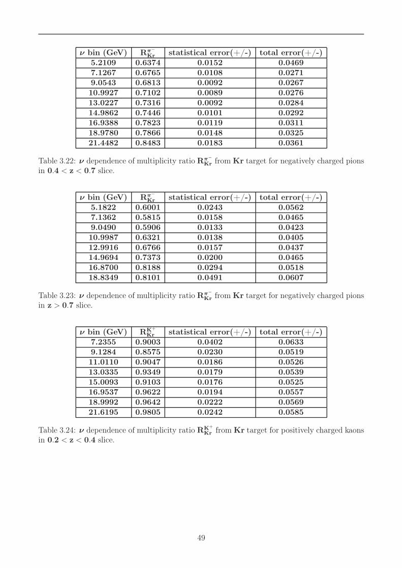
ν bin (GeV) Rπ−
Kr statistical error(+/-) total error(+/-)5.2109 0.6374 0.0152 0.04697.1267 0.6765 0.0108 0.02719.0543 0.6813 0.0092 0.026710.9927 0.7102 0.0089 0.027613.0227 0.7316 0.0092 0.028414.9862 0.7446 0.0101 0.029216.9388 0.7823 0.0119 0.031118.9780 0.7866 0.0148 0.032521.4482 0.8483 0.0183 0.0361
Table 3.22: ν dependence of multiplicity ratio Rπ−
Kr from Kr target for negatively charged pionsin 0.4 < z < 0.7 slice.
ν bin (GeV) Rπ−
Kr statistical error(+/-) total error(+/-)5.1822 0.6001 0.0243 0.05627.1362 0.5815 0.0158 0.04659.0490 0.5906 0.0133 0.042310.9987 0.6321 0.0138 0.040512.9916 0.6766 0.0157 0.043714.9694 0.7373 0.0200 0.046516.8700 0.8188 0.0294 0.051818.8349 0.8101 0.0491 0.0607
Table 3.23: ν dependence of multiplicity ratio Rπ−
Kr from Kr target for negatively charged pionsin z > 0.7 slice.
ν bin (GeV) RK+
Kr statistical error(+/-) total error(+/-)7.2355 0.9003 0.0402 0.06339.1284 0.8575 0.0230 0.051911.0110 0.9047 0.0186 0.052613.0335 0.9349 0.0179 0.053915.0093 0.9103 0.0176 0.052516.9537 0.9622 0.0194 0.055718.9992 0.9642 0.0222 0.056921.6195 0.9805 0.0242 0.0585
Table 3.24: ν dependence of multiplicity ratio RK+
Kr from Kr target for positively charged kaonsin 0.2 < z < 0.4 slice.
49

ν bin (GeV) RK+
Kr statistical error(+/-) total error(+/-)5.2041 0.9065 0.0531 0.07637.1397 0.8368 0.0284 0.05639.0744 0.7539 0.0194 0.045311.0096 0.7936 0.0175 0.046513.0210 0.8073 0.0176 0.047214.9816 0.8497 0.0195 0.050116.9737 0.8394 0.0222 0.050718.9584 0.8911 0.0284 0.056121.4285 0.8948 0.0331 0.0588
Table 3.25: ν dependence of multiplicity ratio RK+
Kr from Kr target for positively charged kaonsin 0.4 < z < 0.7 slice.
ν bin (GeV) RK+
Kr statistical error(+/-) total error(+/-)5.1716 0.7450 0.0669 0.08057.1397 0.7675 0.0408 0.05839.0541 0.7357 0.0319 0.051111.0317 0.7002 0.0295 0.048113.0304 0.6849 0.0306 0.048214.9763 0.7529 0.0358 0.054316.9284 0.7492 0.0457 0.061218.8397 0.7964 0.0747 0.0863
Table 3.26: ν dependence of multiplicity ratio RK+
Kr from Kr target for positively charged kaonsin z > 0.7 slice.
ν bin (GeV) RK−
Kr statistical error(+/-) total error(+/-)7.4250 0.6566 0.0503 0.06179.1531 0.6934 0.0290 0.047511.0468 0.7240 0.0227 0.045413.0198 0.7766 0.0221 0.047615.0068 0.7923 0.0224 0.048516.9798 0.8427 0.0242 0.051819.0035 0.8722 0.0281 0.051121.5910 0.9165 0.0297 0.0518
Table 3.27: ν dependence of multiplicity ratio RK−
Kr from Kr target for negatively chargedkaons in 0.2 < z < 0.4 slice.
50

ν bin (GeV) RK−
Kr statistical error(+/-) total error(+/-)5.2834 0.6103 0.0725 0.07597.1634 0.6493 0.0406 0.04409.1178 0.6124 0.0295 0.033511.0337 0.7104 0.0286 0.034012.9731 0.7190 0.0281 0.033715.0066 0.7575 0.0303 0.036116.9519 0.8033 0.0360 0.041618.9638 0.7662 0.0412 0.045721.4876 0.8786 0.0496 0.0546
Table 3.28: ν dependence of multiplicity ratio RK−
Kr from Kr target for negatively chargedkaons in 0.4 < z < 0.7 slice.
ν bin (GeV) RK−
Kr statistical error(+/-) total error(+/-)5.2556 0.4421 0.1567 0.15917.1119 0.4453 0.0939 0.09709.0790 0.6974 0.1014 0.108911.1358 0.7142 0.0894 0.097513.1244 0.6999 0.0819 0.090314.9903 0.5874 0.0733 0.080016.9105 0.6624 0.0928 0.099618.9913 0.7328 0.1474 0.1527
Table 3.29: ν dependence of multiplicity ratio RK−
Kr from Kr target for negatively chargedkaons in z > 0.7 slice.
ν bin (GeV) RpKr statistical error(+/-) total error(+/-)
7.2579 0.9065 0.0226 0.04859.0946 0.9845 0.0177 0.049911.0043 1.1217 0.0180 0.056213.0356 1.1268 0.0180 0.056214.9793 1.1792 0.0194 0.058916.9465 1.2389 0.0228 0.062718.9883 1.2593 0.0277 0.065521.5344 1.2380 0.0298 0.0656
Table 3.30: ν dependence of multiplicity ratio RpKr from Kr target for protons in 0.2 < z < 0.4
slice.
51

ν bin (GeV) RpKr statistical error(+/-) total error(+/-)
5.2030 0.7948 0.0169 0.06737.0134 0.8735 0.0156 0.04419.0200 0.9078 0.0174 0.046210.9823 0.8938 0.0184 0.046012.9931 0.9270 0.0202 0.048214.9600 0.9220 0.0221 0.048816.9347 0.9599 0.0266 0.052518.9820 0.9015 0.0324 0.053521.4726 0.9927 0.0424 0.0632
Table 3.31: ν dependence of multiplicity ratio RpKr from Kr target for protons in 0.4 < z < 0.7
slice.
ν bin (GeV) Rp
Kr statistical error(+/-) total error(+/-)4.9596 0.7995 0.0393 0.07647.0072 0.7425 0.0414 0.05428.9614 0.7733 0.0456 0.058410.9638 0.8037 0.0486 0.061613.0004 0.7406 0.0522 0.062814.9801 0.6231 0.0587 0.065616.9239 0.7412 0.0937 0.100118.8191 0.5236 0.1035 0.1066
Table 3.32: ν dependence of multiplicity ratio Rp
Kr from Kr target for protons in z > 0.7 slice.
ν bin (GeV) Rp̄
Kr statistical error(+/-) total error(+/-)7.3000 0.7001 0.0616 0.09849.1244 0.5809 0.0413 0.084411.0179 0.7183 0.0473 0.092213.1124 0.6113 0.0336 0.076614.9892 0.7553 0.0346 0.092516.9559 0.7599 0.0358 0.090619.0176 0.8160 0.0407 0.098221.6592 0.8594 0.0444 0.1041
Table 3.33: ν dependence of multiplicity ratio Rp̄
Kr from Kr target for antiprotons in0.2 < z < 0.4 slice.
52

ν bin (GeV) Rp̄Kr statistical error(+/-) total error(+/-)
5.1554 0.6879 0.0615 0.10777.0032 0.6186 0.0568 0.08849.0117 0.5683 0.0559 0.083711.0475 0.6618 0.0563 0.091813.0547 0.6626 0.0528 0.089815.0543 0.7541 0.0584 0.101216.9606 0.6210 0.0507 0.084818.9729 0.7123 0.0646 0.101321.5611 0.6503 0.0712 0.1007
Table 3.34: ν dependence of multiplicity ratio Rp̄
Kr from Kr target for antiprotons in0.4 < z < 0.7 slice.
ν bin (GeV) Rπ+
Xe statistical error(+/-) total error(+/-)5.6308 0.6328 0.0460 0.06367.2467 0.6377 0.0132 0.02729.1288 0.6538 0.0084 0.026411.0234 0.6928 0.0072 0.027513.0436 0.7244 0.0069 0.028614.9990 0.7468 0.0072 0.029116.9641 0.7601 0.0078 0.029718.9900 0.7768 0.0091 0.030721.5390 0.8380 0.0101 0.0332
Table 3.35: ν dependence of multiplicity ratio Rπ+
Xe from Xe target for positively charged pionsin 0.2 < z < 0.4 slice.
ν bin (GeV) Rπ+
Xe statistical error(+/-) total error(+/-)5.2548 0.5913 0.0164 0.04347.1235 0.6011 0.0108 0.02299.0671 0.6112 0.0091 0.022411.0140 0.6505 0.0089 0.023613.0002 0.6781 0.0091 0.024514.9798 0.6913 0.0100 0.025316.9450 0.7232 0.0118 0.027018.9383 0.7551 0.0150 0.029421.3881 0.7865 0.0183 0.0321
Table 3.36: ν dependence of multiplicity ratio Rπ+
Xe from Xe target for positively charged pions0.4 < z < 0.7 slice.
53

ν bin (GeV) Rπ+
Xe statistical error(+/-) total error(+/-)5.2297 0.5726 0.0243 0.05107.1501 0.5261 0.0153 0.03109.0573 0.5332 0.0130 0.029110.9828 0.5447 0.0130 0.028213.0034 0.5932 0.0148 0.031014.9347 0.6186 0.0181 0.031916.8801 0.6767 0.0259 0.037218.8148 0.6861 0.0434 0.0499
Table 3.37: ν dependence of multiplicity ratio Rπ+
Xe from Xe target for positively charged pionsz > 0.7 slice.
ν bin (GeV) Rπ−
Xe statistical error(+/-) total error(+/-)5.6299 0.6745 0.0496 0.07027.2676 0.6378 0.0141 0.03259.1417 0.6716 0.0092 0.033211.0208 0.7043 0.0079 0.035413.0282 0.7258 0.0076 0.036315.0101 0.7350 0.0078 0.037316.9691 0.7594 0.0085 0.038718.9790 0.7842 0.0099 0.040221.5287 0.8196 0.0108 0.0421
Table 3.38: ν dependence of multiplicity ratio Rπ−
Xe from Xe target for negaitively chargedpions in 0.2 < z < 0.4 slice.
ν bin (GeV) Rπ−
Xe statistical error(+/-) total error(+/-)5.2051 0.5842 0.0172 0.04467.1152 0.6317 0.0123 0.02719.0490 0.6403 0.0106 0.026710.9844 0.6502 0.0101 0.026913.0210 0.6824 0.0106 0.028214.9856 0.7202 0.0118 0.030016.9331 0.7291 0.0135 0.031018.9506 0.7486 0.0171 0.033421.3593 0.7810 0.0204 0.0362
Table 3.39: ν dependence of multiplicity ratio Rπ−
Xe from Xe target for negatively charged pionsin 0.4 < z < 0.7 slice.
54

ν bin (GeV) Rπ−
Xe statistical error(+/-) total error(+/-)5.2650 0.5567 0.0276 0.05517.1230 0.5301 0.0180 0.04689.0794 0.5477 0.0153 0.044810.9894 0.5908 0.0157 0.039812.9766 0.5999 0.0175 0.041114.9438 0.7026 0.0231 0.047216.8477 0.6928 0.0317 0.049218.7900 0.7178 0.0542 0.0643
Table 3.40: ν dependence of multiplicity ratio Rπ−
Xe from Xe target for negatively charged pionsin z > 0.7 slice.
ν bin (GeV) RK+
Xe statistical error(+/-) total error(+/-)7.3590 0.8114 0.0468 0.06439.1282 0.8191 0.0271 0.052111.0318 0.8331 0.0213 0.050013.0319 0.8818 0.0206 0.052114.9979 0.8734 0.0204 0.051616.9643 0.9175 0.0222 0.054519.0014 0.9305 0.0259 0.056821.5107 0.9750 0.0283 0.0601
Table 3.41: ν dependence of multiplicity ratio RK+
Xe from Xe target for positively charged kaonsin 0.2 < z < 0.4 slice.
ν bin (GeV) RK+
Xe statistical error(+/-) total error(+/-)5.3125 0.9034 0.0656 0.08557.1648 0.7814 0.0327 0.05369.0798 0.7502 0.0231 0.046811.0198 0.7176 0.0196 0.043613.0073 0.7770 0.0204 0.046914.9690 0.7998 0.0224 0.048916.9267 0.8032 0.0257 0.050618.9699 0.8435 0.0327 0.056321.3959 0.9216 0.0400 0.0641
Table 3.42: ν dependence of multiplicity ratio RK+
Xe from Xe target for positively charged kaonsin 0.4 < z < 0.7 slice.
55

ν bin (GeV) RK+
Xe statistical error(+/-) total error(+/-)4.9942 0.6713 0.0755 0.08567.1071 0.7059 0.0458 0.05979.0090 0.6691 0.0358 0.051010.8859 0.6548 0.0336 0.048913.0619 0.6634 0.0361 0.051014.9570 0.6445 0.0390 0.052416.8175 0.7016 0.0517 0.064218.9207 0.7464 0.0858 0.0949
Table 3.43: ν dependence of multiplicity ratio RK+
Xe from Xe target for positively charged kaonsin z > 0.7 slice.
ν bin (GeV) RK−
Xe statistical error(+/-) total error(+/-)7.3407 0.6079 0.0580 0.06679.1573 0.6292 0.0332 0.047611.0686 0.6937 0.0264 0.046013.0031 0.7171 0.0251 0.046314.9962 0.7878 0.0267 0.050416.9755 0.7665 0.0270 0.049619.0117 0.8501 0.0329 0.056721.5575 0.8593 0.0338 0.0576
Table 3.44: ν dependence of multiplicity ratio RK−
Xe from Xe target for negatively chargedkaons in 0.2 < z < 0.4 slice.
ν bin (GeV) RK−
Xe statistical error(+/-) total error(+/-)5.2496 0.5979 0.0834 0.09087.0871 0.4981 0.0417 0.04979.1005 0.5718 0.0342 0.046211.0014 0.6581 0.0326 0.048413.0759 0.6783 0.0324 0.049114.9444 0.6998 0.0343 0.051216.9388 0.7727 0.0418 0.059318.9894 0.6847 0.0459 0.059121.5187 0.8244 0.0574 0.0728
Table 3.45: ν dependence of multiplicity ratio RK−
Xe from Xe target for negatively chargedkaons in 0.4 < z < 0.7 slice.
56

ν bin (GeV) RK−
Xe statistical error(+/-) total error(+/-)4.8000 0.3977 0.1811 0.18276.9000 0.5300 0.1190 0.12248.6500 0.5282 0.0936 0.097910.6500 0.6069 0.0937 0.099313.4000 0.6939 0.0969 0.104014.8500 0.6061 0.0865 0.092616.5000 0.7106 0.1000 0.107218.3000 0.7375 0.1410 0.1466
Table 3.46: ν dependence of multiplicity ratio RK−
Xe from Xe target for negatively chargedkaons in z > 0.7 slice.
ν bin (GeV) RpXe statistical error(+/-) total error(+/-)
7.2556 0.8859 0.0262 0.04959.0956 0.9748 0.0205 0.050711.0030 1.0747 0.0205 0.055013.0184 1.1526 0.0214 0.058614.9774 1.1880 0.0228 0.060516.9513 1.2226 0.0264 0.063418.9702 1.2976 0.0330 0.069521.4798 1.3014 0.0359 0.0711
Table 3.47: ν dependence of multiplicity ratio Rp
Xe from Xe target for protons in 0.2 < z < 0.4slice.
ν bin (GeV) RpXe statistical error(+/-) total error(+/-)
5.1914 0.7535 0.0195 0.06487.0335 0.8131 0.0177 0.04229.0193 0.9063 0.0206 0.047510.9647 0.8505 0.0211 0.045312.9707 0.8675 0.0229 0.046914.9515 0.8628 0.0252 0.047916.9037 0.8989 0.0302 0.052118.8929 0.9446 0.0392 0.059421.3710 0.9986 0.0498 0.0686
Table 3.48: ν dependence of multiplicity ratio Rp
Xe from Xe target for protons in 0.4 < z < 0.7slice.
57
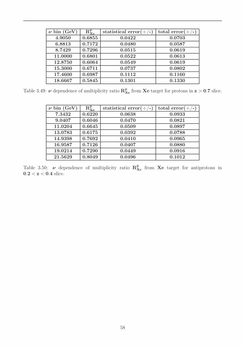
ν bin (GeV) RpXe statistical error(+/-) total error(+/-)
4.9050 0.6855 0.0422 0.07036.8813 0.7172 0.0480 0.05878.7429 0.7296 0.0515 0.061911.0000 0.6801 0.0522 0.061312.8750 0.6064 0.0549 0.061915.3000 0.6711 0.0737 0.080217.4600 0.6987 0.1112 0.116018.6667 0.5845 0.1301 0.1330
Table 3.49: ν dependence of multiplicity ratio RpXe from Xe target for protons in z > 0.7 slice.
ν bin (GeV) Rp̄
Xe statistical error(+/-) total error(+/-)7.3432 0.6220 0.0638 0.09339.0407 0.6046 0.0470 0.082111.0204 0.6645 0.0509 0.089713.0783 0.6175 0.0392 0.078814.9398 0.7692 0.0410 0.096516.9587 0.7126 0.0407 0.088019.0214 0.7290 0.0449 0.091621.5629 0.8049 0.0496 0.1012
Table 3.50: ν dependence of multiplicity ratio Rp̄Xe from Xe target for antiprotons in
0.2 < z < 0.4 slice.
58

ν bin (GeV) Rp̄Xe statistical error(+/-) total error(+/-)
5.2183 0.5288 0.0613 0.09166.9205 0.6454 0.0670 0.09759.0711 0.6025 0.0681 0.094811.0510 0.3983 0.0500 0.066413.0575 0.6018 0.0598 0.089015.0186 0.7427 0.0677 0.105816.9382 0.6021 0.0592 0.088619.1057 0.6459 0.0721 0.101021.5546 0.7488 0.0902 0.1219
Table 3.51: ν dependence of multiplicity ratio Rp̄
Xe from Xe target for antiprotons in0.4 < z < 0.7 slice.
3.2 z dependence in three ν slices
In Figure 3.2, the dependence of RhA on z for three slices in ν is presented. The large
attenuation at high z values explains differently in different phenomenology models. In parton
energy loss modell this phenomena caused by the strong decrease of the fragmentation function
at high z range while in absorbtion type models this is assumed to be a result of a decreasment
of the formation length leading to the large energy losses in the nuclear medium.
0.2
0.4
0.6
0.8
1
1.2
0 0.5 1
0.2
0.4
0.6
0.8
1
1.2
0 0.5 1
0.2
0.4
0.6
0.8
1
1.2
0 0.5 1
0.5
1
1.5
0 0.5 1
0.5
1
1.5
0 0.5 1
0.5
1
1.5
0 0.5 1
0.5
1
1.5
0 0.5 1
0.5
1
1.5
0 0.5 1
ν = 4-12 GeVν = 12-17 GeVν = 17-23.5 GeV
0.4
0.6
1.0
0.8
RAh
Ne Kr
π+
Xe
1.5
0.5
1.0
K+
0.5
1.0
1.5
0.5 1 0.5 1 10.5
p
z
0.5
1
1.5
0 0.5 1
0.2
0.4
0.6
0.8
1
1.2
0 0.5 1
0.2
0.4
0.6
0.8
1
1.2
0 0.5 1
0.2
0.4
0.6
0.8
1
1.2
0 0.5 1
0.5
1
1.5
0 0.5 1
0.5
1
1.5
0 0.5 1
0.5
1
1.5
0 0.5 1
0.5
1
1.5
0 0.5 1
0.5
1
1.5
0 0.5 1
ν = 4-12 GeVν = 12-17 GeVν = 17-23.5 GeV
0.4
0.6
1.0
0.8
RAh
Ne Kr
π-
Xe
1.5
0.5
1.0
K -
0.5
1.0
1.5
0.5 1 0.5 1 10.5
p–
z
0.5
1
1.5
0 0.5 1
Figure 3.2: Dependence of RhA on z for three slices in ν.
Looking on experimental data one can see that the RhA shows a slight change in different
59
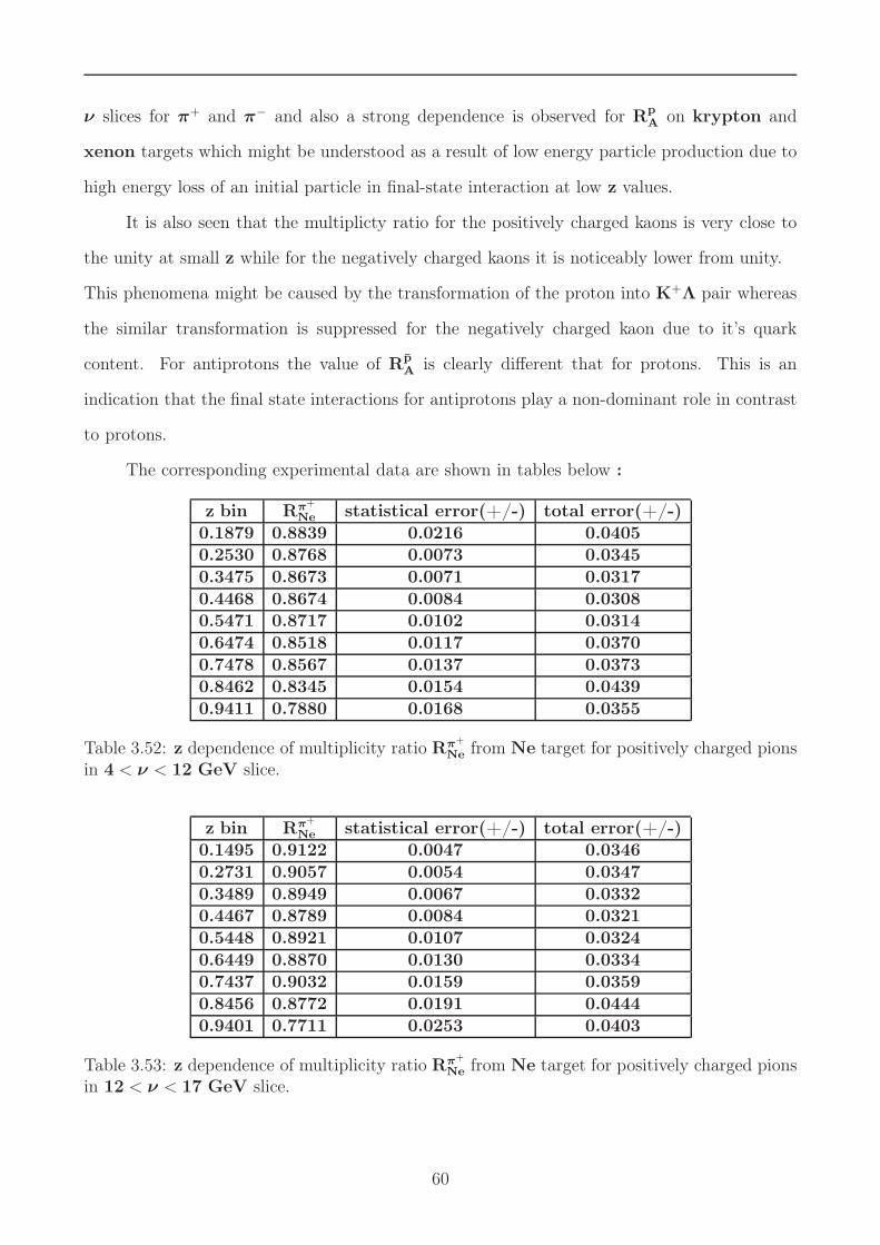
ν slices for π+ and π− and also a strong dependence is observed for RpA on krypton and
xenon targets which might be understood as a result of low energy particle production due to
high energy loss of an initial particle in final-state interaction at low z values.
It is also seen that the multiplicty ratio for the positively charged kaons is very close to
the unity at small z while for the negatively charged kaons it is noticeably lower from unity.
This phenomena might be caused by the transformation of the proton into K+Λ pair whereas
the similar transformation is suppressed for the negatively charged kaon due to it’s quark
content. For antiprotons the value of Rp̄A is clearly different that for protons. This is an
indication that the final state interactions for antiprotons play a non-dominant role in contrast
to protons.
The corresponding experimental data are shown in tables below :
z bin Rπ+
Ne statistical error(+/-) total error(+/-)0.1879 0.8839 0.0216 0.04050.2530 0.8768 0.0073 0.03450.3475 0.8673 0.0071 0.03170.4468 0.8674 0.0084 0.03080.5471 0.8717 0.0102 0.03140.6474 0.8518 0.0117 0.03700.7478 0.8567 0.0137 0.03730.8462 0.8345 0.0154 0.04390.9411 0.7880 0.0168 0.0355
Table 3.52: z dependence of multiplicity ratio Rπ+
Ne from Ne target for positively charged pionsin 4 < ν < 12 GeV slice.
z bin Rπ+
Ne statistical error(+/-) total error(+/-)0.1495 0.9122 0.0047 0.03460.2731 0.9057 0.0054 0.03470.3489 0.8949 0.0067 0.03320.4467 0.8789 0.0084 0.03210.5448 0.8921 0.0107 0.03240.6449 0.8870 0.0130 0.03340.7437 0.9032 0.0159 0.03590.8456 0.8772 0.0191 0.04440.9401 0.7711 0.0253 0.0403
Table 3.53: z dependence of multiplicity ratio Rπ+
Ne from Ne target for positively charged pionsin 12 < ν < 17 GeV slice.
60

z bin Rπ+
Ne statistical error(+/-) total error(+/-)0.0950 0.9376 0.0161 0.03800.1492 0.9290 0.0031 0.03500.2731 0.9233 0.0055 0.03530.3489 0.9177 0.0076 0.03420.4467 0.9179 0.0104 0.03400.5448 0.9456 0.0142 0.03540.6449 0.9419 0.0186 0.03760.7437 0.9501 0.0291 0.04460.8456 0.8874 0.0661 0.0775
Table 3.54: z dependence of multiplicity ratio Rπ+
Ne from Ne target for positively charged pionsin 17 < ν < 23.5 GeV slice.
z bin Rπ−
Ne statistical error(+/-) total error(+/-)0.1877 0.8777 0.0234 0.04520.2529 0.8612 0.0079 0.03900.3472 0.8501 0.0078 0.03620.4466 0.8616 0.0093 0.03370.5468 0.8593 0.0113 0.03350.6479 0.8362 0.0133 0.03410.7477 0.8532 0.0157 0.04000.8482 0.8180 0.0174 0.05680.9416 0.7680 0.0188 0.0465
Table 3.55: z dependence of multiplicity ratio Rπ−
Ne from Ne target for negatively charged pionsin 4 < ν < 12 GeV slice.
z bin Rπ−
Ne statistical error(+/-) total error(+/-)0.1495 0.9052 0.0051 0.04020.2729 0.8897 0.0058 0.03990.3440 0.8853 0.0075 0.03750.4451 0.8928 0.0097 0.03490.5438 0.8864 0.0124 0.03480.6440 0.8963 0.0154 0.03710.7482 0.8814 0.0185 0.04220.8288 0.9180 0.0234 0.06510.9579 0.8433 0.0326 0.0569
Table 3.56: z dependence of multiplicity ratio Rπ−
Ne from Ne target for negatively charged pionsin 12 < ν < 17 GeV slice.
61

z bin Rπ−
Ne statistical error(+/-) total error(+/-)0.0950 0.9192 0.0168 0.04320.1495 0.9109 0.0033 0.04020.2729 0.9128 0.0059 0.04090.3440 0.9178 0.0083 0.03900.4451 0.9133 0.0116 0.03620.5438 0.9024 0.0157 0.03660.6440 0.9323 0.0218 0.04130.7482 0.9404 0.0342 0.05300.8288 0.9724 0.0857 0.1071
Table 3.57: z dependence of multiplicity ratio Rπ−
Ne from Ne target for negatively charged pionsin 17 < ν < 23.5 GeV slice.
z bin RK+
Ne statistical error(+/-) total error(+/-)0.1902 1.1529 0.0980 0.15000.2567 0.9135 0.0202 0.05670.3479 0.9717 0.0196 0.05770.4453 0.9181 0.0202 0.05380.5473 0.9352 0.0231 0.05710.6482 0.9194 0.0269 0.05730.7480 0.9041 0.0315 0.05860.8427 0.7948 0.0350 0.05770.9467 0.7936 0.0480 0.0656
Table 3.58: z dependence of multiplicity ratio RK+
Ne from Ne target for positively charged kaonsin 4 < ν < 12 GeV slice.
z bin RK+
Ne statistical error(+/-) total error(+/-)0.1495 0.9696 0.0148 0.05600.2731 0.9751 0.0154 0.05650.3489 0.9689 0.0164 0.05640.4467 0.9401 0.0181 0.05540.5448 0.9097 0.0212 0.05500.6449 0.9282 0.0271 0.05840.7437 0.8392 0.0309 0.05610.8456 0.8399 0.0401 0.06160.9401 0.7114 0.0600 0.0719
Table 3.59: z dependence of multiplicity ratio RK+
Ne from Ne target for positively charged kaonsin 12 < ν < 17 GeV slice.
62

z bin RK+
Ne statistical error(+/-) total error(+/-)0.0950 0.9403 0.0759 0.09300.1495 0.9795 0.0105 0.05710.2731 0.9879 0.0157 0.05870.3489 0.9462 0.0172 0.05680.4467 0.9307 0.0215 0.05750.5448 0.9298 0.0268 0.05960.6449 0.9684 0.0355 0.06580.7437 0.9965 0.0590 0.08210.8456 0.6996 0.1032 0.1107
Table 3.60: z dependence of multiplicity ratio RK+
Ne from Ne target for positively charged kaonsin 17 < ν < 23.5 GeV slice.
z bin RK−
Ne statistical error(+/-) total error(+/-)0.1909 0.7802 0.1061 0.11870.2551 0.8546 0.0279 0.06460.3467 0.8284 0.0256 0.06210.4446 0.8333 0.0299 0.06420.5462 0.7968 0.0364 0.06540.6413 0.7449 0.0476 0.06960.7412 0.7498 0.0728 0.08900.8416 0.8210 0.1480 0.15820.9383 0.5553 0.2324 0.2355
Table 3.61: z dependence of multiplicity ratio RK−
Ne from Ne target for negatively charged kaonsin 4 < ν < 12 GeV slice.
z bin RK−
Ne statistical error(+/-) total error(+/-)0.1495 0.8822 0.0181 0.06290.2729 0.8893 0.0191 0.06360.3440 0.8470 0.0215 0.06170.4451 0.8912 0.0283 0.06710.5438 0.9184 0.0366 0.07260.6440 0.7410 0.0451 0.06780.7482 0.8119 0.0709 0.09000.8288 0.6173 0.0935 0.1026
Table 3.62: z dependence of multiplicity ratio RK−
Ne from Ne target for negatively charged kaonsin 12 < ν < 17 GeV slice.
63

z bin RK−
Ne statistical error(+/-) total error(+/-)0.1495 0.9303 0.0125 0.06470.2729 0.9129 0.0186 0.06500.3440 0.9213 0.0239 0.06730.4451 0.9245 0.0326 0.07100.5438 0.8796 0.0410 0.07270.6440 0.8046 0.0547 0.07750.7482 0.8718 0.1034 0.11930.8288 1.1076 0.3473 0.3555
Table 3.63: z dependence of multiplicity ratio RK−
Ne from Ne target for negatively charged kaonsin 17 < ν < 23.5 GeV slice.
z bin RpNe statistical error(+/-) total error(+/-)
0.2731 1.0638 0.0276 0.05770.3489 1.0178 0.0137 0.05050.4467 1.0138 0.0147 0.05340.5448 0.9793 0.0177 0.05070.6449 0.9358 0.0233 0.05030.7437 0.9606 0.0351 0.05840.8456 0.9124 0.0529 0.06930.9401 0.7690 0.0652 0.0750
Table 3.64: z dependence of multiplicity ratio Rp
Ne from Ne target for protons in 4 < ν < 12
GeV slice.
z bin Rp
Ne statistical error(+/-) total error(+/-)0.2731 1.0922 0.0165 0.05650.3489 1.0407 0.0165 0.05410.4467 0.9836 0.0196 0.05250.5448 0.9571 0.0250 0.05360.6449 0.9504 0.0346 0.05840.7437 1.0489 0.0577 0.07760.8456 0.8918 0.0953 0.10500.9401 0.8156 0.2144 0.2182
Table 3.65: z dependence of multiplicity ratio Rp
Ne from Ne target for protons in 12 < ν < 17
GeV slice.
z bin Rp
Ne statistical error(+/-) total error(+/-)0.2731 1.1017 0.0173 0.05720.3489 1.0106 0.0200 0.05380.4467 0.9992 0.0248 0.05530.5448 0.9539 0.0332 0.05770.6449 0.9499 0.0521 0.07020.7437 0.9990 0.1023 0.1136
Table 3.66: z dependence of multiplicity ratio RpNe from Ne target for protons in 17 < ν < 23.5
GeV slice.
64
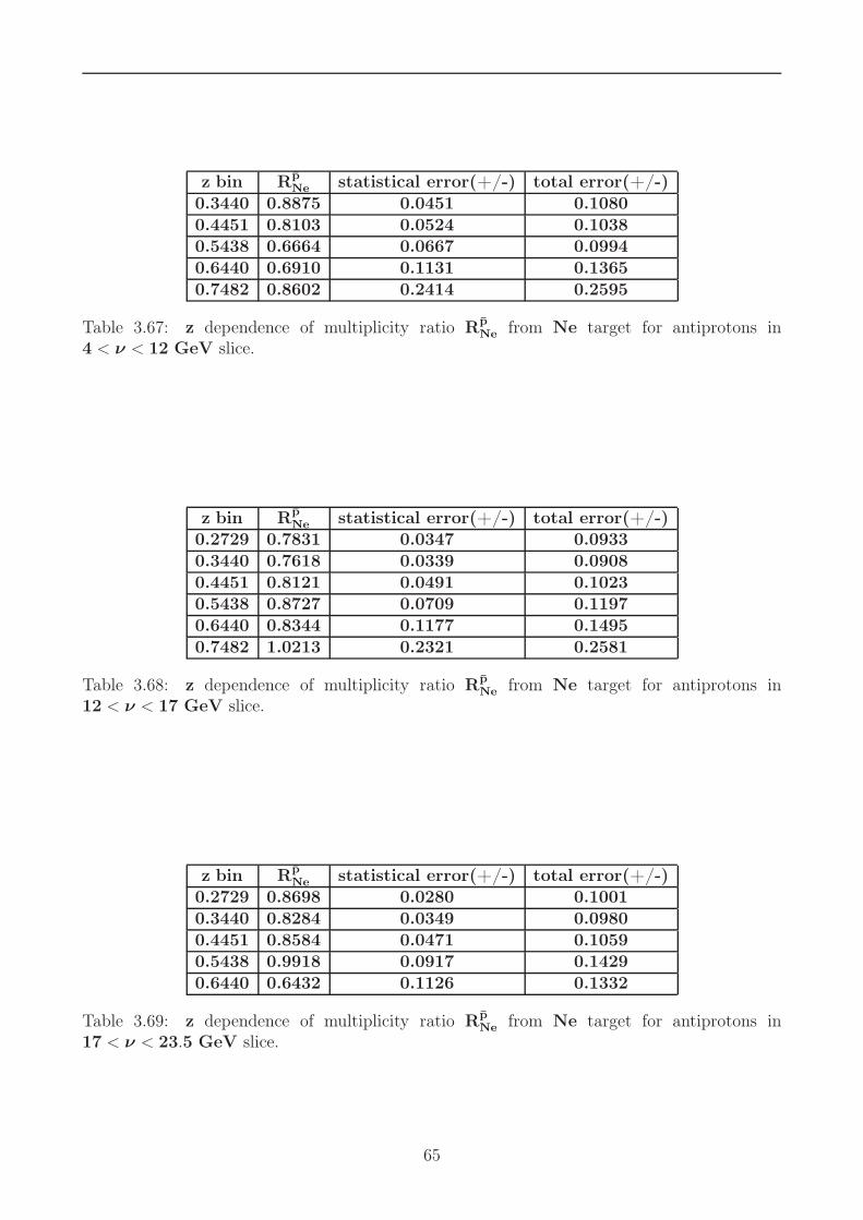
z bin Rp̄Ne statistical error(+/-) total error(+/-)
0.3440 0.8875 0.0451 0.10800.4451 0.8103 0.0524 0.10380.5438 0.6664 0.0667 0.09940.6440 0.6910 0.1131 0.13650.7482 0.8602 0.2414 0.2595
Table 3.67: z dependence of multiplicity ratio Rp̄
Ne from Ne target for antiprotons in4 < ν < 12 GeV slice.
z bin Rp̄
Ne statistical error(+/-) total error(+/-)0.2729 0.7831 0.0347 0.09330.3440 0.7618 0.0339 0.09080.4451 0.8121 0.0491 0.10230.5438 0.8727 0.0709 0.11970.6440 0.8344 0.1177 0.14950.7482 1.0213 0.2321 0.2581
Table 3.68: z dependence of multiplicity ratio Rp̄
Ne from Ne target for antiprotons in12 < ν < 17 GeV slice.
z bin Rp̄
Ne statistical error(+/-) total error(+/-)0.2729 0.8698 0.0280 0.10010.3440 0.8284 0.0349 0.09800.4451 0.8584 0.0471 0.10590.5438 0.9918 0.0917 0.14290.6440 0.6432 0.1126 0.1332
Table 3.69: z dependence of multiplicity ratio Rp̄Ne from Ne target for antiprotons in
17 < ν < 23.5 GeV slice.
65

z bin Rπ+
Kr statistical error(+/-) total error(+/-)0.1879 0.8213 0.0207 0.03990.2526 0.7563 0.0065 0.03460.3473 0.7310 0.0063 0.03050.4469 0.6988 0.0070 0.03030.5469 0.6949 0.0084 0.02730.6474 0.6705 0.0098 0.03130.7469 0.6366 0.0109 0.03260.8468 0.5925 0.0118 0.03600.9406 0.5390 0.0125 0.0269
Table 3.70: z dependence of multiplicity ratio Rπ+
Kr from Kr target for positively charged pionsin 4 < ν < 12 GeV slice.
z bin Rπ+
Kr statistical error(+/-) total error(+/-)0.1668 0.8341 0.0062 0.03270.2466 0.7979 0.0051 0.03140.3460 0.7726 0.0064 0.02970.4459 0.7603 0.0081 0.02880.5464 0.7328 0.0098 0.02730.6468 0.7257 0.0118 0.02820.7477 0.7007 0.0139 0.02950.8461 0.6641 0.0165 0.03700.9361 0.5775 0.0220 0.0338
Table 3.71: z dependence of multiplicity ratio Rπ+
Kr from Kr target for positively charged pionsin 12 < ν < 17 GeV slice.
z bin Rπ+
Kr statistical error(+/-) total error(+/-)0.0940 0.9506 0.0329 0.04030.1493 0.8885 0.0052 0.02370.2447 0.8552 0.0064 0.02350.3445 0.8456 0.0088 0.02270.4453 0.8363 0.0120 0.02250.5463 0.8211 0.0156 0.02270.6442 0.8236 0.0206 0.02690.7416 0.7242 0.0276 0.03260.8266 0.7269 0.0633 0.0700
Table 3.72: z dependence of multiplicity ratio Rπ+
Kr from Kr target for positively charged pionsin 17 < ν < 23.5 GeV slice.
66

z bin Rπ−
Kr statistical error(+/-) total error(+/-)0.1880 0.7994 0.0214 0.04380.2524 0.7507 0.0070 0.03760.3476 0.7264 0.0068 0.03250.4461 0.6987 0.0078 0.02840.5467 0.6934 0.0095 0.02750.6478 0.6637 0.0110 0.02820.7481 0.6271 0.0124 0.03100.8474 0.6174 0.0141 0.04890.9420 0.5578 0.0149 0.0376
Table 3.73: z dependence of multiplicity ratio Rπ−
Kr from Kr target for negatively charged pionsin 4 < ν < 12 GeV slice.
z bin Rπ−
Kr statistical error(+/-) total error(+/-)0.1665 0.8199 0.0065 0.03970.2468 0.7978 0.0056 0.03970.3454 0.7744 0.0071 0.03460.4459 0.7438 0.0090 0.03040.5458 0.7458 0.0114 0.03000.6469 0.7464 0.0141 0.03240.7465 0.7350 0.0169 0.03740.8450 0.7321 0.0207 0.05920.9357 0.6282 0.0270 0.0473
Table 3.74: z dependence of multiplicity ratio Rπ−
Kr from Kr target for negatively charged pionsin 12 < ν < 17 GeV slice.
z bin Rπ−
Kr statistical error(+/-) total error(+/-)0.0942 0.9156 0.0330 0.05270.1490 0.8771 0.0055 0.04220.2446 0.8411 0.0068 0.04190.3441 0.8315 0.0097 0.03750.4442 0.8167 0.0134 0.03450.5458 0.8046 0.0178 0.03470.6438 0.8098 0.0235 0.03940.7401 0.8241 0.0363 0.05200.8281 0.8256 0.0850 0.1056
Table 3.75: z dependence of multiplicity ratio Rπ−
Kr from Kr target for negatively charged pionsin 17 < ν < 23.5 GeV slice.
67

z bin RK+
Kr statistical error(+/-) total error(+/-)0.1879 1.0689 0.0901 0.10830.2526 0.9263 0.0209 0.05590.3473 0.8656 0.0180 0.05070.4469 0.8405 0.0187 0.05050.5469 0.7750 0.0198 0.04730.6474 0.7507 0.0226 0.04720.7469 0.7501 0.0267 0.04870.8268 0.7611 0.0342 0.05370.9406 0.6321 0.0392 0.0533
Table 3.76: z dependence of multiplicity ratio RK+
Kr from Kr target for positively charged kaonsin 4 < ν < 12 GeV slice.
z bin RK+
Kr statistical error(+/-) total error(+/-)0.1668 0.9860 0.0212 0.05890.2466 0.9900 0.0163 0.05750.3460 0.8621 0.0157 0.05050.4459 0.8310 0.0175 0.04950.5464 0.8301 0.0212 0.05090.6468 0.7953 0.0257 0.05120.7477 0.7298 0.0294 0.05020.8461 0.6897 0.0368 0.05320.9361 0.6815 0.0601 0.0711
Table 3.77: z dependence of multiplicity ratio RK+
Kr from Kr target for positively charged kaonsin 12 < ν < 17 GeV slice.
z bin RK+
Kr statistical error(+/-) total error(+/-)0.0940 1.1955 0.2046 0.21510.1493 1.0967 0.0196 0.06410.2447 0.9847 0.0186 0.05790.3445 0.9536 0.0216 0.05730.4453 0.9018 0.0264 0.05670.5463 0.9011 0.0322 0.05960.6442 0.8528 0.0394 0.06170.7416 0.8229 0.0563 0.07260.8266 0.8575 0.1476 0.1551
Table 3.78: z dependence of multiplicity ratio RK+
Kr from Kr target for positively charged kaonsin 17 < ν < 23.5 GeV slice.
68

z bin RK−
Kr statistical error(+/-) total error(+/-)0.1880 0.8101 0.1073 0.11640.2524 0.7039 0.0243 0.04610.3476 0.7193 0.0236 0.04650.4461 0.6897 0.0261 0.04650.5467 0.6346 0.0301 0.04640.6478 0.6550 0.0440 0.05720.7481 0.6434 0.0637 0.07310.8474 0.6498 0.1165 0.12200.9420 0.5748 0.1952 0.1978
Table 3.79: z dependence of multiplicity ratio RK−
Kr from Kr target for negatively charged kaonsin 4 < ν < 12 GeV slice.
z bin RK−
Kr statistical error(+/-) total error(+/-)0.1665 0.8299 0.0246 0.05240.2468 0.8271 0.0192 0.04990.3454 0.7621 0.0213 0.04750.4459 0.7911 0.0274 0.05190.5458 0.7183 0.0328 0.05180.6469 0.6927 0.0448 0.05910.7465 0.6010 0.0585 0.06740.8450 0.6903 0.0986 0.10580.9357 0.5063 0.1854 0.1875
Table 3.80: z dependence of multiplicity ratio RK−
Kr from Kr target for negatively charged kaonsin 12 < ν < 17 GeV slice.
z bin RK−
Kr statistical error(+/-) total error(+/-)0.1490 0.9384 0.0211 0.05630.2446 0.9058 0.0225 0.05520.3441 0.8458 0.0275 0.05450.4442 0.8409 0.0378 0.06020.5458 0.7849 0.0469 0.06410.6438 0.8080 0.0667 0.08040.7401 0.7413 0.1098 0.11730.8281 0.6688 0.2251 0.2282
Table 3.81: z dependence of multiplicity ratio RK−
Kr from Kr target for negatively charged kaonsin 17 < ν < 23.5 GeV slice.
69

z bin Rp
Kr statistical error(+/-) total error(+/-)0.2526 1.1789 0.0256 0.06460.3473 0.9928 0.0124 0.04860.4469 0.9151 0.0128 0.04780.5469 0.8513 0.0152 0.04920.6474 0.7868 0.0200 0.04450.7469 0.8215 0.0300 0.06010.8468 0.7077 0.0415 0.05450.9406 0.7332 0.0579 0.0766
Table 3.82: z dependence of multiplicity ratio Rp
Kr from Kr target for protons in 4 < ν < 12
GeV slice.
z bin RpKr statistical error(+/-) total error(+/-)
0.2466 1.2042 0.0169 0.06200.3460 1.1111 0.0175 0.05770.4459 0.9865 0.0201 0.05280.5464 0.8945 0.0238 0.05030.6468 0.8336 0.0317 0.05200.7477 0.7183 0.0442 0.05670.8461 0.7136 0.0846 0.09170.9361 0.5388 0.1403 0.1428
Table 3.83: z dependence of multiplicity ratio RpKr from Kr target for protons in 12 < ν < 17
GeV slice.
z bin RpKr statistical error(+/-) total error(+/-)
0.2447 1.3258 0.0232 0.06950.3445 1.1448 0.0263 0.06230.4453 1.0302 0.0301 0.05910.5463 0.8420 0.0366 0.05540.6442 0.8331 0.0564 0.06980.7416 0.6062 0.0858 0.0909
Table 3.84: z dependence of multiplicity ratio Rp
Kr from Kr target for protons in 17 < ν < 23.5GeV slice.
z bin Rp̄Kr statistical error(+/-) total error(+/-)
0.3476 0.6822 0.0289 0.08080.4461 0.6316 0.0370 0.07900.5467 0.6500 0.0583 0.09250.6478 0.6158 0.0933 0.11550.7481 0.2719 0.1021 0.1064
Table 3.85: z dependence of multiplicity ratio Rp̄
Kr from Kr target for antiprotons in 4 < ν < 12
GeV slice.
70

z bin Rp̄Kr statistical error(+/-) total error(+/-)
0.2468 0.7242 0.0297 0.08540.3454 0.6522 0.0308 0.07840.4459 0.6490 0.0433 0.08380.5458 0.7357 0.0639 0.10340.6469 0.6959 0.1019 0.12770.7465 0.7466 0.2266 0.2412
Table 3.86: z dependence of multiplicity ratio Rp̄Kr from Kr target for antiprotons in
12 < ν < 17 GeV slice.
z bin Rp̄
Kr statistical error(+/-) total error(+/-)0.2446 0.8421 0.0325 0.09860.3441 0.8318 0.0436 0.10180.4442 0.7071 0.0509 0.09330.5458 0.6394 0.0754 0.10330.6438 0.5671 0.1141 0.1302
Table 3.87: z dependence of multiplicity ratio Rp̄Kr from Kr target for antiprotons in
17 < ν < 23.5 GeV slice.
z bin Rπ+
Xe statistical error(+/-) total error(+/-)0.1900 0.7511 0.0177 0.04790.2724 0.6938 0.0075 0.03710.3486 0.6591 0.0070 0.03280.4464 0.6313 0.0078 0.03100.5456 0.6314 0.0095 0.02670.6442 0.6040 0.0110 0.02830.7437 0.5951 0.0124 0.02830.8437 0.5375 0.0133 0.03590.9385 0.4590 0.0136 0.0264
Table 3.88: z dependence of multiplicity ratio Rπ+
Xe from Xe target for positively charged pionsin 4 < ν < 12 GeV slice.
71

z bin Rπ+
Xe statistical error(+/-) total error(+/-)0.1666 0.8001 0.0073 0.03210.2467 0.7462 0.0059 0.03090.3463 0.7265 0.0073 0.02890.4459 0.7080 0.0092 0.02730.5468 0.6795 0.0112 0.02610.6473 0.6540 0.0132 0.02660.7464 0.6397 0.0157 0.02850.8453 0.5953 0.0185 0.03620.9374 0.5530 0.0257 0.0363
Table 3.89: z dependence of multiplicity ratio Rπ+
Xe from Xe target for positively charged pionsin 12 < ν < 17 GeV slice.
z bin Rπ+
Xe statistical error(+/-) total error(+/-)0.0950 0.8960 0.0190 0.03930.1666 0.8512 0.0050 0.03350.2467 0.8058 0.0062 0.03330.3463 0.7892 0.0085 0.03150.4459 0.7775 0.0116 0.03050.5468 0.7572 0.0151 0.03030.6473 0.7349 0.0197 0.03250.7464 0.6843 0.0284 0.03810.8453 0.7668 0.0725 0.0828
Table 3.90: z dependence of multiplicity ratio Rπ+
Xe from Xe target for positively charged pionsin 17 < ν < 23.5 GeV slice.
z bin Rπ−
Xe statistical error(+/-) total error(+/-)0.1900 0.7481 0.0183 0.04110.2733 0.6986 0.0081 0.03680.3441 0.6783 0.0078 0.03150.4450 0.6460 0.0088 0.02700.5430 0.6427 0.0108 0.02730.6460 0.6208 0.0128 0.02800.7524 0.5868 0.0143 0.03220.8550 0.5641 0.0146 0.04860.9675 0.5200 0.0154 0.0377
Table 3.91: z dependence of multiplicity ratio Rπ−
Xe from Xe target for negatively charged pionsin 4 < ν < 12 GeV slice.
72

z bin Rπ−
Xe statistical error(+/-) total error(+/-)0.1665 0.7963 0.0077 0.03990.2469 0.7448 0.0064 0.03880.3454 0.7154 0.0080 0.03320.4459 0.7105 0.0104 0.03000.5461 0.7179 0.0133 0.03100.6467 0.6823 0.0159 0.03170.7450 0.6542 0.0187 0.03720.8464 0.6617 0.0233 0.05910.9365 0.6203 0.0322 0.0522
Table 3.92: z dependence of multiplicity ratio Rπ−
Xe from Xe target for negatively charged pionsin 12 < ν < 17 GeV slice.
z bin Rπ−
Xe statistical error(+/-) total error(+/-)0.0950 0.8862 0.0193 0.04580.1665 0.8521 0.0053 0.04220.2469 0.8034 0.0066 0.04180.3454 0.7783 0.0092 0.03620.4459 0.7654 0.0129 0.03290.5461 0.7439 0.0172 0.03370.6467 0.7308 0.0226 0.03700.7450 0.7213 0.0359 0.05040.8464 0.6479 0.0809 0.0968
Table 3.93: z dependence of multiplicity ratio Rπ−
Xe from Xe target for negatively charged pionsin 17 < ν < 23.5 GeV slice.
z bin RK+
Xe statistical error(+/-) total error(+/-)0.1850 1.0556 0.0802 0.10020.2724 0.8860 0.0247 0.05450.3486 0.7851 0.0204 0.04800.4464 0.7989 0.0215 0.05240.5456 0.7245 0.0225 0.04760.6442 0.7059 0.0260 0.04910.7437 0.7092 0.0306 0.04920.8437 0.6570 0.0370 0.05170.9385 0.6107 0.0452 0.0564
Table 3.94: z dependence of multiplicity ratio RK+
Xe from Xe target for positively charged kaonsin 4 < ν < 12 GeV slice.
73
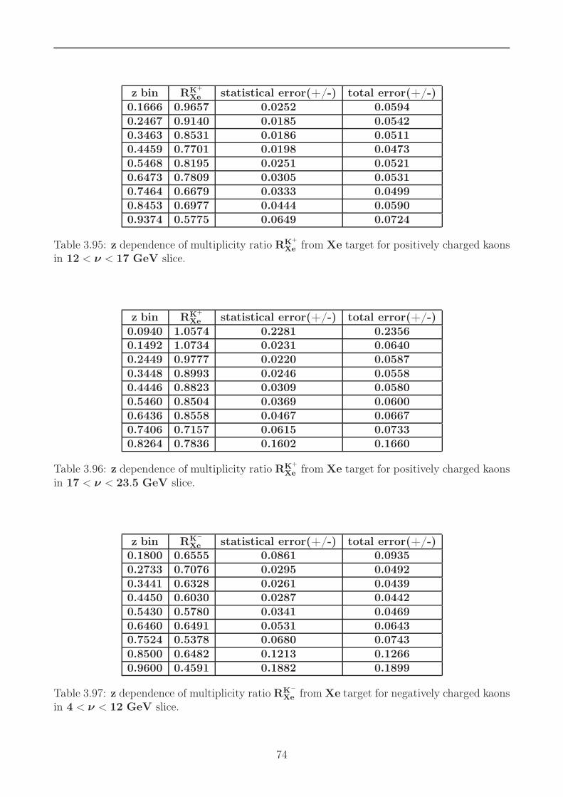
z bin RK+
Xe statistical error(+/-) total error(+/-)0.1666 0.9657 0.0252 0.05940.2467 0.9140 0.0185 0.05420.3463 0.8531 0.0186 0.05110.4459 0.7701 0.0198 0.04730.5468 0.8195 0.0251 0.05210.6473 0.7809 0.0305 0.05310.7464 0.6679 0.0333 0.04990.8453 0.6977 0.0444 0.05900.9374 0.5775 0.0649 0.0724
Table 3.95: z dependence of multiplicity ratio RK+
Xe from Xe target for positively charged kaonsin 12 < ν < 17 GeV slice.
z bin RK+
Xe statistical error(+/-) total error(+/-)0.0940 1.0574 0.2281 0.23560.1492 1.0734 0.0231 0.06400.2449 0.9777 0.0220 0.05870.3448 0.8993 0.0246 0.05580.4446 0.8823 0.0309 0.05800.5460 0.8504 0.0369 0.06000.6436 0.8558 0.0467 0.06670.7406 0.7157 0.0615 0.07330.8264 0.7836 0.1602 0.1660
Table 3.96: z dependence of multiplicity ratio RK+
Xe from Xe target for positively charged kaonsin 17 < ν < 23.5 GeV slice.
z bin RK−
Xe statistical error(+/-) total error(+/-)0.1800 0.6555 0.0861 0.09350.2733 0.7076 0.0295 0.04920.3441 0.6328 0.0261 0.04390.4450 0.6030 0.0287 0.04420.5430 0.5780 0.0341 0.04690.6460 0.6491 0.0531 0.06430.7524 0.5378 0.0680 0.07430.8500 0.6482 0.1213 0.12660.9600 0.4591 0.1882 0.1899
Table 3.97: z dependence of multiplicity ratio RK−
Xe from Xe target for negatively charged kaonsin 4 < ν < 12 GeV slice.
74

z bin RK−
Xe statistical error(+/-) total error(+/-)0.1665 0.8565 0.0300 0.05640.2469 0.7503 0.0216 0.04710.3454 0.7553 0.0253 0.04910.4459 0.7113 0.0305 0.05000.5461 0.7097 0.0390 0.05550.6467 0.6750 0.0527 0.06480.7450 0.6690 0.0741 0.08300.8464 0.6296 0.1087 0.11420.9365 0.6817 0.2375 0.2405
Table 3.98: z dependence of multiplicity ratio RK−
Xe from Xe target for negatively charged kaonsin 12 < ν < 17 GeV slice.
z bin RK−
Xe statistical error(+/-) total error(+/-)0.1489 0.9067 0.0246 0.05610.2441 0.8687 0.0261 0.05490.3440 0.7889 0.0312 0.05390.4455 0.7687 0.0426 0.06040.5442 0.7659 0.0556 0.07000.6427 0.7058 0.0731 0.08300.7393 0.6219 0.1182 0.12310.8207 0.8448 0.3095 0.3131
Table 3.99: z dependence of multiplicity ratio RK−
Xe from Xe target for negatively charged kaonsin 17 < ν < 23.5 GeV slice.
z bin RpXe statistical error(+/-) total error(+/-)
0.2724 1.1469 0.0292 0.06760.3486 0.9654 0.0142 0.03200.4464 0.8875 0.0148 0.03370.5456 0.8142 0.0175 0.03640.6442 0.7244 0.0226 0.03570.7437 0.7160 0.0323 0.05050.8437 0.7528 0.0506 0.05830.9385 0.5498 0.0579 0.0638
Table 3.100: z dependence of multiplicity ratio Rp
Xe from Xe target for protons in 4 < ν < 12
GeV slice.
75

z bin Rp
Xe statistical error(+/-) total error(+/-)0.2467 1.2364 0.0200 0.06440.3463 1.1004 0.0205 0.05820.4459 0.9592 0.0234 0.05290.5468 0.8062 0.0265 0.04790.6473 0.7511 0.0347 0.05090.7464 0.6250 0.0485 0.05750.8453 0.6689 0.0972 0.10270.9374 0.5420 0.1647 0.1669
Table 3.101: z dependence of multiplicity ratio Rp
Xe from Xe target for protons in 12 < ν < 17
GeV slice.
z bin RpXe statistical error(+/-) total error(+/-)
0.2449 1.3770 0.0278 0.07350.3448 1.1427 0.0308 0.06430.4446 1.0017 0.0347 0.06040.5460 0.8968 0.0452 0.06330.6436 0.7954 0.0653 0.07620.7406 0.6603 0.1076 0.1125
Table 3.102: z dependence of multiplicity ratio Rp
Xe from Xe target for protons in17 < ν < 23.5 GeV slice.
z bin Rp̄
Xe statistical error(+/-) total error(+/-)0.3441 0.6079 0.0309 0.07400.4450 0.5323 0.0389 0.07050.5430 0.5370 0.0609 0.08510.6460 0.5720 0.1066 0.12390.7524 0.4146 0.1490 0.1559
Table 3.103: z dependence of multiplicity ratio Rp̄Xe from Xe target for antiprotons in
4 < ν < 12 GeV slice.
76

z bin Rp̄Xe statistical error(+/-) total error(+/-)
0.2469 0.7447 0.0350 0.08950.3454 0.6402 0.0362 0.07950.4459 0.6617 0.0525 0.09000.5461 0.7246 0.0746 0.10950.6467 0.5668 0.1044 0.12180.7450 0.3331 0.1614 0.1655
Table 3.104: z dependence of multiplicity ratio Rp̄Xe from Xe target for antiprotons in
12 < ν < 17 GeV slice.
z bin Rp̄
Xe statistical error(+/-) total error(+/-)0.2441 0.7334 0.0351 0.08810.3440 0.8179 0.0508 0.10350.4455 0.6796 0.0587 0.09520.5442 0.6573 0.0905 0.11590.6427 0.5777 0.1394 0.1532
Table 3.105: z dependence of multiplicity ratio Rp̄Xe from Xe target for antiprotons in
17 < ν < 23.5 GeV slice.
77

3.3 p2t dependence in three z slices
The dependence of RhA on p2
t is shown in Figure 3.3 for three slices in z. An increasing
behaviour of RhA was observed at high p2
t (the Cronin effect[37]) which is larger for protons
compared with mesons. This effect depends also on target mass which was observed by the
HERMES collaboration before[38].
0
0.5
1
1.5
2
2.5
10-2 10-1 1
0
0.5
1
1.5
2
2.5
10-2 10-1 1
0
0.5
1
1.5
2
2.5
10-2 10-1 1
0
0.5
1
1.5
2
2.5
10-2 10-1 1
0
0.5
1
1.5
2
2.5
10-2 10-1 1
0
0.5
1
1.5
2
2.5
10-2 10-1 1
0
0.5
1
1.5
2
2.5
10-2 10-1 1
0
0.5
1
1.5
2
2.5
10-2 10-1 1
z = 0.2-0.4z = 0.4-0.7z > 0.7
0.5
1.0
1.5
2.0
RAh
Ne Kr
π+
Xe
0.5
1.0
1.5
2.0
2.5
K+
0.5
1.0
1.5
0
2.0
2.5
0.1 1 0.1 1 10.1
p
pt2 [GeV2]
0
0.5
1
1.5
2
2.5
10-2 10-1 1
Figure 3.3: Dependence of RhA on p2
t for three slices in z.
In contrast to heavy ion collision experiments[37] the lepton-nucleon interaction is not
contributed by the initial state interaction. The observed enhancment of RhA assumed the pt
broadening due to the multiple scattering of the struck quark and also the interaction of pro-
duced hadron with nuclear enviorement. There are different phenomenological models[39],[40]
trying to explain the Cronin effect.
What we see in our data, for the highest z slice the Cronin effect is suppressed for
mesons while the protons show a significant rise with p2t . Such a suppression reveals a partonic
origin of the trasnverse momentum broadening. The point is that at high z the partonic energy
loss is highly suppressed[11]. Due to the limited statistics only the data for positively charged
hadrons are presented. The related tables for Figure 3.3 are presented below :
78

p2t (GeV2) Rπ+
Ne statistical error(+/-) total error(+/-)0.0232 0.8786 0.0053 0.03210.0737 0.8899 0.0067 0.03270.1840 0.8965 0.0048 0.03260.3826 0.9134 0.0088 0.03410.5836 0.9303 0.0167 0.03740.7845 0.9645 0.0311 0.04660.9841 0.9304 0.0524 0.06221.2206 1.1266 0.0946 0.10291.6532 1.0512 0.1484 0.1532
Table 3.106: p2t dependence of multiplicity ratio Rπ+
Ne from Ne target for positively chargedpions in 0.2 < z < 0.4 slice.
p2t (GeV2) Rπ+
Ne statistical error(+/-) total error(+/-)0.0243 0.8516 0.0082 0.02930.0745 0.8992 0.0096 0.03120.1830 0.8984 0.0065 0.03040.3889 0.8667 0.0103 0.03040.5890 0.8752 0.0151 0.03260.7887 0.8929 0.0224 0.03700.9913 0.9117 0.0316 0.04361.2278 0.9326 0.0397 0.05021.8093 1.0538 0.0533 0.0636
Table 3.107: p2t dependence of multiplicity ratio Rπ+
Ne from Ne target for positively chargedpions in 0.4 < z < 0.7 slice.
p2t (GeV2) Rπ+
Ne statistical error(+/-) total error(+/-)0.0242 0.8966 0.0150 0.03770.0734 0.9262 0.0178 0.03990.1823 0.8178 0.0112 0.03350.3872 0.8198 0.0184 0.03660.5883 0.8297 0.0281 0.04260.7904 0.8375 0.0413 0.05240.9872 0.8920 0.0601 0.06921.2293 0.7837 0.0601 0.06731.8417 0.8714 0.0787 0.0856
Table 3.108: p2t dependence of multiplicity ratio Rπ+
Ne from Ne target for positively chargedpions in z > 0.7 slice.
79

p2t (GeV2) RK+
Ne statistical error(+/-) total error(+/-)0.0230 0.9360 0.0137 0.05260.0735 0.9310 0.0180 0.05360.1848 0.9537 0.0130 0.05340.3846 1.0062 0.0229 0.05930.5845 1.0386 0.0411 0.06970.7869 1.0498 0.0706 0.09030.9816 1.0823 0.1180 0.13171.2093 1.1914 0.1870 0.19641.6596 0.8037 0.2149 0.2174
Table 3.109: p2t dependence of multiplicity ratio RK+
Ne from Ne target for positively chargedkaons in 0.2 < z < 0.4 slice.
p2t (GeV2) RK+
Ne statistical error(+/-) total error(+/-)0.0236 0.9585 0.0191 0.05540.0740 0.8905 0.0208 0.05260.1860 0.9074 0.0142 0.05130.3888 0.9108 0.0215 0.05390.5919 0.9501 0.0310 0.06010.7902 0.9416 0.0429 0.06080.9882 0.9522 0.0605 0.07971.2241 1.0426 0.0768 0.09461.8255 1.0760 0.0916 0.1086
Table 3.110: p2t dependence of multiplicity ratio RK+
Ne from Ne target for positively chargedkaons in 0.4 < z < 0.7 slice.
p2t (GeV2) RK+
Ne statistical error(+/-) total error(+/-)0.0241 0.9056 0.0413 0.06420.0737 0.8758 0.0441 0.06470.1859 0.8304 0.0259 0.05200.3873 0.7966 0.0353 0.05580.5882 0.8256 0.0512 0.06750.7972 0.9455 0.0800 0.09460.9910 0.8477 0.0957 0.10601.2284 0.8375 0.1164 0.12441.8673 0.9063 0.1316 0.1386
Table 3.111: p2t dependence of multiplicity ratio RK+
Ne from Ne target for positively chargedkaons in z > 0.7 slice.
80
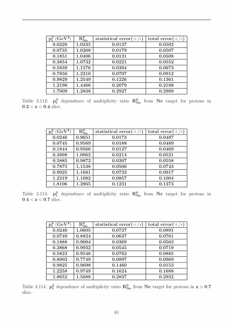
p2t (GeV2) R
p
Ne statistical error(+/-) total error(+/-)0.0228 1.0235 0.0137 0.05020.0735 1.0268 0.0179 0.05070.1851 1.0406 0.0131 0.05080.3854 1.0732 0.0221 0.05520.5839 1.1576 0.0394 0.06730.7856 1.2210 0.0707 0.09120.9829 1.2549 0.1226 0.13611.2198 1.4466 0.2079 0.21881.7009 1.2838 0.2927 0.2989
Table 3.112: p2t dependence of multiplicity ratio R
p
Ne from Ne target for protons in0.2 < z < 0.4 slice.
p2t (GeV2) Rp
Ne statistical error(+/-) total error(+/-)0.0246 0.9651 0.0173 0.04870.0745 0.9569 0.0188 0.04890.1844 0.9566 0.0127 0.04690.3898 1.0062 0.0214 0.05210.5885 0.9872 0.0307 0.05580.7875 1.1538 0.0506 0.07430.9925 1.1681 0.0733 0.09171.2219 1.1082 0.0857 0.10041.8106 1.2865 0.1231 0.1373
Table 3.113: p2t dependence of multiplicity ratio Rp
Ne from Ne target for protons in0.4 < z < 0.7 slice.
p2t (GeV2) Rp
Ne statistical error(+/-) total error(+/-)0.0240 1.0605 0.0737 0.08910.0749 0.8824 0.0637 0.07610.1888 0.9004 0.0369 0.05630.3868 0.9932 0.0545 0.07190.5823 0.9546 0.0762 0.08850.8002 0.7749 0.0897 0.09690.9825 0.9698 0.1460 0.01531.2258 0.9749 0.1624 0.16881.8652 1.5688 0.2837 0.2932
Table 3.114: p2t dependence of multiplicity ratio Rp
Ne from Ne target for protons in z > 0.7slice.
81

p2t (GeV2) Rπ+
Kr statistical error(+/-) total error(+/-)0.0231 0.7581 0.0046 0.02840.0739 0.7652 0.0058 0.02890.1844 0.7926 0.0042 0.02960.3833 0.8504 0.0080 0.03240.5841 0.9040 0.0156 0.03690.7848 0.9500 0.0289 0.04550.9852 1.0776 0.0548 0.06781.2196 1.1418 0.0845 0.09451.6453 1.3170 0.1643 0.1714
Table 3.115: p2t dependence of multiplicity ratio Rπ+
Kr from Kr target for positively chargedpions in 0.2 < z < 0.4 slice.
p2t (GeV2) Rπ+
Kr statistical error(+/-) total error(+/-)0.0241 0.6943 0.0071 0.02430.0745 0.7158 0.0079 0.02530.1816 0.7462 0.0055 0.02560.3885 0.7256 0.0088 0.02590.5895 0.7649 0.0133 0.02890.7889 0.8126 0.0199 0.03370.9902 0.8704 0.0296 0.04161.2287 0.8971 0.0372 0.04781.8148 1.1383 0.0522 0.0647
Table 3.116: p2t dependence of multiplicity ratio Rπ+
Kr from Kr target for positively chargedpions in 0.4 < z < 0.7 slice.
p2t (GeV2) Rπ+
Kr statistical error(+/-) total error(+/-)0.0244 0.6648 0.0118 0.03020.0736 0.6711 0.0138 0.03130.1808 0.6106 0.0089 0.02710.3868 0.5797 0.0142 0.02810.5870 0.6052 0.0220 0.03360.7901 0.6483 0.0322 0.04210.9924 0.5853 0.0418 0.04851.2226 0.6511 0.0531 0.05971.9074 0.8015 0.0690 0.0767
Table 3.117: p2t dependence of multiplicity ratio Rπ+
Kr from Kr target for positively chargedpions in z > 0.7 slice.
82

p2t (GeV2) RK+
Kr statistical error(+/-) total error(+/-)0.0230 0.8459 0.0125 0.04760.0735 0.8651 0.0166 0.04980.1866 0.9466 0.0126 0.05290.3832 1.0321 0.0224 0.06040.5867 1.0910 0.0401 0.07160.7884 1.2239 0.0767 0.10150.9798 1.2764 0.1239 0.14201.2088 1.0759 0.1505 0.16151.7124 1.6546 0.3399 0.3516
Table 3.118: p2t dependence of multiplicity ratio RK+
Kr from Kr target for positively chargedkaons in 0.2 < z < 0.4 slice.
p2t (GeV2) RK+
Kr statistical error(+/-) total error(+/-)0.0236 0.7897 0.0162 0.04580.0743 0.7808 0.0185 0.04630.1867 0.8053 0.0128 0.04560.3897 0.8402 0.0197 0.04970.5896 0.8747 0.0280 0.05510.7906 0.9029 0.0406 0.06370.9900 0.9667 0.0569 0.07741.2313 1.0558 0.0722 0.09221.8626 1.2160 0.0947 0.1155
Table 3.119: p2t dependence of multiplicity ratio RK+
Kr from Kr target for positively chargedkaons in 0.4 < z < 0.7 slice.
p2t (GeV2) RK+
Kr statistical error(+/-) total error(+/-)0.0239 0.8122 0.0373 0.05780.0753 0.7271 0.0376 0.05450.1875 0.7263 0.0227 0.04550.3891 0.7120 0.0318 0.05010.5885 0.6031 0.0398 0.05150.7908 0.6438 0.0592 0.06880.9979 0.8581 0.0943 0.10521.2207 0.8150 0.1036 0.11271.7916 1.0173 0.1426 0.1529
Table 3.120: p2t dependence of multiplicity ratio RK+
Kr from Kr target for positively chargedkaons in z > 0.7 slice.
83

p2t (GeV2) Rp
Kr statistical error(+/-) total error(+/-)0.0230 1.0529 0.0129 0.05150.0733 1.0673 0.0169 0.05320.1857 1.1224 0.0126 0.05450.3863 1.2401 0.0223 0.06260.5843 1.4514 0.0427 0.08070.7857 1.6064 0.0779 0.10870.9826 1.6831 0.1350 0.15661.2239 1.6862 0.1987 0.21401.6638 1.9557 0.3579 0.3696
Table 3.121: p2t dependence of multiplicity ratio Rp
Kr from Kr target for protons in0.2 < z < 0.4 slice.
p2t (GeV2) Rp
Kr statistical error(+/-) total error(+/-)0.0250 0.8405 0.0149 0.04240.0746 0.8514 0.0163 0.04330.1835 0.8147 0.0106 0.03990.3903 0.9210 0.0186 0.04730.5910 1.0408 0.0294 0.05720.7879 1.2434 0.0479 0.07570.9926 1.3612 0.0754 0.09901.2289 1.6749 0.1085 0.13421.8849 2.1867 0.1653 0.1949
Table 3.122: p2t dependence of multiplicity ratio Rp
Kr from Kr target for protons in0.4 < z < 0.7 slice.
p2t (GeV2) Rp
Kr statistical error(+/-) total error(+/-)0.0253 0.6855 0.0497 0.05930.0756 0.7289 0.0531 0.06330.1893 0.7469 0.0304 0.04650.3904 0.7081 0.0397 0.05190.5933 0.6960 0.0557 0.06470.7865 0.7431 0.0815 0.08871.0052 0.9366 0.1327 0.13991.2259 1.1314 0.1724 0.18051.8090 1.5900 0.2520 0.2629
Table 3.123: p2t dependence of multiplicity ratio Rp
Kr from Kr target for protons in z > 0.7slice.
84

p2t (GeV2) Rπ+
Xe statistical error(+/-) total error(+/-)0.0232 0.6979 0.0038 0.02700.0736 0.7101 0.0048 0.02760.1849 0.7402 0.0034 0.02850.3834 0.8049 0.0063 0.03150.5833 0.8784 0.0121 0.03570.7836 0.9450 0.0222 0.04250.9867 1.1131 0.0426 0.06031.2179 1.1361 0.0631 0.07661.6966 1.5603 0.1302 0.1433
Table 3.124: p2t dependence of multiplicity ratio Rπ+
Xe from Xe target for positively chargedpions in 0.2 < z < 0.4 slice.
p2t (GeV2) Rπ+
Xe statistical error(+/-) total error(+/-)0.0241 0.6394 0.0059 0.02220.0744 0.6462 0.0066 0.02270.1843 0.6796 0.0045 0.02320.3888 0.6711 0.0071 0.02360.5892 0.6928 0.0104 0.02550.7906 0.7520 0.0156 0.02970.9895 0.8285 0.0232 0.03621.2313 0.9456 0.0304 0.04391.8261 1.1169 0.0404 0.0551
Table 3.125: p2t dependence of multiplicity ratio Rπ+
Xe from Xe target for positively chargedpions in 0.4 < z < 0.7 slice.
p2t (GeV2) Rπ+
Xe statistical error(+/-) total error(+/-)0.0245 0.5793 0.0097 0.02680.0744 0.6253 0.0118 0.02950.1819 0.5590 0.0076 0.02530.3867 0.5464 0.0122 0.02660.5920 0.5572 0.0184 0.03030.7887 0.5976 0.0268 0.03720.9953 0.5960 0.0374 0.04541.2186 0.6457 0.0455 0.05341.8794 0.6673 0.0526 0.0600
Table 3.126: p2t dependence of multiplicity ratio Rπ+
Xe from Xe target for positively chargedpions in z > 0.7 slice.
85

p2t (GeV2) RK+
Xe statistical error(+/-) total error(+/-)0.0230 0.8011 0.0105 0.04280.0733 0.8059 0.0133 0.04580.1857 0.8799 0.0099 0.04880.3847 1.0743 0.0187 0.06130.5837 1.1214 0.0323 0.06890.7830 1.1292 0.0545 0.08200.9898 1.3820 0.0996 0.12471.2299 1.5173 0.1419 0.16411.6920 2.2071 0.2902 0.3140
Table 3.127: p2t dependence of multiplicity ratio RK+
Xe from Xe target for positively chargedkaons in 0.2 < z < 0.4 slice.
p2t (GeV2) RK+
Xe statistical error(+/-) total error(+/-)0.0241 0.7505 0.0138 0.04300.0736 0.7133 0.0153 0.04170.1872 0.7667 0.0106 0.04300.3886 0.7848 0.0158 0.04550.5887 0.8452 0.0229 0.05130.7886 0.9617 0.0351 0.06290.9872 1.0200 0.0479 0.07321.2296 1.1638 0.0622 0.08871.8430 1.3336 0.0771 0.1058
Table 3.128: p2t dependence of multiplicity ratio RK+
Xe from Xe target for positively chargedkaons in 0.4 < z < 0.7 slice.
p2t (GeV2) RK+
Xe statistical error(+/-) total error(+/-)0.0246 0.7471 0.0318 0.05160.0748 0.7240 0.0331 0.05140.1913 0.6716 0.0192 0.04120.3921 0.5923 0.0250 0.04070.5940 0.6505 0.0369 0.05110.7867 0.7328 0.0551 0.06800.9908 0.6034 0.0654 0.07321.2278 0.6563 0.0784 0.08611.8511 0.6937 0.0948 0.1020
Table 3.129: p2t dependence of multiplicity ratio RK+
Xe from Xe target for positively chargedkaons in z > 0.7 slice.
86

p2t (GeV2) R
p
Xe statistical error(+/-) total error(+/-)0.0229 1.0277 0.0110 0.04990.0733 1.0891 0.0145 0.05350.1869 1.1223 0.0104 0.05400.3868 1.2834 0.0185 0.06330.5852 1.4665 0.0341 0.07710.7818 1.7241 0.0632 0.10300.9880 1.8321 0.1064 0.13711.2243 1.9304 0.1556 0.18031.6849 1.9529 0.2451 0.2618
Table 3.130: p2t dependence of multiplicity ratio R
p
Xe from Xe target for protons in0.2 < z < 0.4 slice.
p2t (GeV2) Rp
Xe statistical error(+/-) total error(+/-)0.0237 0.8030 0.0129 0.04000.0741 0.7821 0.0139 0.03940.1852 0.7912 0.0093 0.03850.3873 0.8859 0.0159 0.04470.5875 1.0222 0.0253 0.05450.7953 1.1658 0.0397 0.06780.9886 1.4557 0.0668 0.09581.2212 1.5131 0.0836 0.10991.8790 2.1137 0.01303 0.1641
Table 3.131: p2t dependence of multiplicity ratio Rp
Xe from Xe target for protons in0.4 < z < 0.7 slice.
p2t (GeV2) Rp
Xe statistical error(+/-) total error(+/-)0.0239 0.8227 0.0497 0.06310.0755 0.5273 0.0404 0.04740.1927 0.6385 0.0252 0.03930.3852 0.6421 0.0344 0.04580.5910 0.6375 0.0483 0.05690.7872 0.7213 0.0731 0.08060.9877 0.9305 0.1204 0.12821.2329 1.0112 0.1530 0.16032.0002 1.6100 0.2291 0.2414
Table 3.132: p2t dependence of multiplicity ratio Rp
Xe from Xe target for protons in z > 0.7slice.
87

3.4 z dependence in three p2t slices
The z dependence of RhA for three slices in p2
t is presented in Figure 3.4. The overall
reduction of RhA with z was observed. At high p2
t range the z dependence is stronger which
is more prominent for havier targets. At small values of z a strong dependence of RhA on p2
t
0.2
0.4
0.6
0.8
1
1.2
0 0.5 1
0.2
0.4
0.6
0.8
1
1.2
0 0.5 1
0.2
0.4
0.6
0.8
1
1.2
0 0.5 1
0.5
1
1.5
0 0.5 1
0.5
1
1.5
0 0.5 1
0.5
1
1.5
0 0.5 1
0
0.5
1
1.5
2
2.5
0 0.5 1
0
0.5
1
1.5
2
2.5
0 0.5 1
pt2 < 0.4 GeV2
pt2 = 0.4-0.7 GeV2
pt2 > 0.7 GeV2
0.4
0.6
1.0
0.8
RAh
Ne Kr
π+
Xe
1.5
0.5
1.0
K+
0.5
1.5
1.0
0
2.5
2.0
0.5 1 0.5 1 0.5 1
p
z
0
0.5
1
1.5
2
2.5
0 0.5 1
0.2
0.4
0.6
0.8
1
1.2
0 0.5 1
0.2
0.4
0.6
0.8
1
1.2
0 0.5 1
0.2
0.4
0.6
0.8
1
1.2
0 0.5 1
0.5
1
1.5
0 0.5 1
0.5
1
1.5
0 0.5 1
0.5
1
1.5
0 0.5 1
0
0.5
1
1.5
2
2.5
0 0.5 1
0
0.5
1
1.5
2
2.5
0 0.5 1
pt2 < 0.4 GeV2
pt2 = 0.4-0.7 GeV2
pt2 > 0.7 GeV2
0.4
0.6
1.0
0.8
RAh
Ne Kr
π-
Xe
1.5
0.5
1.0
K -
0.5
1.5
1.0
2.5
0
2.0
10.5 10.5 10.5
p–
z
0
0.5
1
1.5
2
2.5
0 0.5 1
Figure 3.4: Dependence of RhA on z for three slices in p2
t .
was found while for high z values there is almost no p2t dependence for π+, π− and K+. This
consistency between different pt values at high z range can be caused by the instantaneous
hadronization since the main contribution into hadron transverse momentum assumed to be
from quark rescatering process which is proportional to the production time and according to
the LUND model it behaves as ∼ (1− z). Thus with increasing of z this time goes down
reducing the contribution from partonic effects into the hadronization process. That is why the
pt dependence disappears at high values of z. The corresponding data points shown in Figure
3.4 are tabulated in tables together with statistical and total errors.
88

z bin Rπ+
Ne statistical error(+/-) total error(+/-)0.0940 0.9236 0.0317 0.04560.1560 0.9089 0.0041 0.03320.2467 0.8978 0.0039 0.03300.3457 0.8793 0.0047 0.03110.4461 0.8748 0.0061 0.03020.5464 0.8879 0.0077 0.03010.6470 0.8933 0.0095 0.03120.7468 0.8939 0.0115 0.03270.8461 0.8695 0.0136 0.04110.9400 0.7813 0.0152 0.0343
Table 3.133: z dependence of multiplicity ratio Rπ+
Ne from Ne target for positively charged pionsin 0.0 < p2
t < 0.4 GeV2 slice.
z bin Rπ+
Ne statistical error(+/-) total error(+/-)0.1813 0.9924 0.0503 0.06190.2552 0.9101 0.0166 0.03710.3481 0.9412 0.0152 0.03710.4465 0.9009 0.0167 0.03620.5466 0.8800 0.0201 0.03480.6457 0.8237 0.0224 0.03520.7449 0.8508 0.0287 0.03540.8426 0.7789 0.0346 0.04090.9418 0.7868 0.0474 0.0566
Table 3.134: z dependence of multiplicity ratio Rπ+
Ne from Ne target for positively charged pionsin 0.4 < p2
t < 0.7 GeV2 slice.
z bin Rπ+
Ne statistical error(+/-) total error(+/-)0.2647 1.0281 0.0513 0.06350.3529 0.9585 0.0294 0.04460.4496 0.9287 0.0256 0.04050.5480 0.9682 0.0280 0.04230.6448 0.8541 0.0292 0.04070.7443 0.8616 0.0375 0.04770.8413 0.7920 0.0498 0.06100.9348 0.8769 0.0737 0.0814
Table 3.135: z dependence of multiplicity ratio Rπ+
Ne from Ne target for positively charged pionsin p2
t > 0.7 GeV2 slice.
89

z bin Rπ−
Ne statistical error(+/-) total error(+/-)0.0941 0.9082 0.0301 0.04870.1555 0.8954 0.0042 0.03860.2459 0.8809 0.0041 0.03830.3453 0.8717 0.0052 0.03550.4459 0.8760 0.0068 0.03250.5465 0.8669 0.0085 0.03180.6470 0.8846 0.0107 0.03380.7469 0.8901 0.0129 0.03940.8470 0.8739 0.0152 0.05910.9410 0.7912 0.0174 0.0464
Table 3.136: z dependence of multiplicity ratio Rπ−
Ne from Ne target for negatively chargedpions in 0.0 < p2
t < 0.4 GeV2 slice.
z bin Rπ−
Ne statistical error(+/-) total error(+/-)0.1820 0.9010 0.0463 0.06030.2543 0.9393 0.0172 0.04410.3481 0.9063 0.0154 0.03960.4460 0.8908 0.0180 0.03700.5450 0.8945 0.0234 0.03930.6458 0.8176 0.0271 0.04020.7435 0.7659 0.0338 0.04660.8428 0.7373 0.0454 0.06620.9399 0.7504 0.0630 0.0751
Table 3.137: z dependence of multiplicity ratio Rπ−
Ne from Ne target for negatively chargedpions in 0.4 < p2
t < 0.7 GeV2 slice.
z bin Rπ−
Ne statistical error(+/-) total error(+/-)0.2648 1.0469 0.0511 0.06820.3532 0.9759 0.0297 0.04930.4485 0.9534 0.0273 0.04400.5475 0.9428 0.0304 0.04510.6453 0.8615 0.0344 0.04650.7422 0.8419 0.0484 0.05990.8415 0.8951 0.0768 0.09660.9386 0.8979 0.0960 0.1077
Table 3.138: z dependence of multiplicity ratio Rπ−
Ne from Ne target for negatively chargedpions in p2
t > 0.7 GeV2 slice.
90

z bin RK+
Ne statistical error(+/-) total error(+/-)0.0949 0.9308 0.1533 0.16140.1589 0.9643 0.0133 0.05400.2494 0.9501 0.0109 0.05270.3479 0.9460 0.0119 0.05270.4469 0.9204 0.0138 0.05190.5465 0.9110 0.0164 0.05210.6462 0.9359 0.0210 0.05500.7457 0.8934 0.0257 0.05490.8350 0.8256 0.0313 0.05470.9377 0.7698 0.0445 0.0611
Table 3.139: z dependence of multiplicity ratio RK+
Ne from Ne target for positively chargedkaons in 0.0 < p2
t < 0.4 GeV2 slice.
z bin RK+
Ne statistical error(+/-) total error(+/-)0.1815 1.0619 0.1392 0.15070.2571 1.0542 0.0456 0.07320.3505 1.0009 0.0350 0.06470.4488 0.9402 0.0351 0.06200.5470 0.9165 0.0391 0.06330.6467 0.8694 0.0438 0.06440.7477 0.8244 0.0503 0.06730.8425 0.7398 0.0630 0.07470.9334 0.7703 0.0958 0.1045
Table 3.140: z dependence of multiplicity ratio RK+
Ne from Ne target for positively chargedkaons in 0.4 < p2
t < 0.7 GeV2 slice.
z bin RK+
Ne statistical error(+/-) total error(+/-)0.2640 1.1601 0.1267 0.14150.3553 1.0333 0.0623 0.08380.4501 0.9621 0.0497 0.07210.5498 0.9947 0.0515 0.07460.6457 0.9853 0.0567 0.07800.7440 0.9668 0.0705 0.08790.8446 0.8174 0.0834 0.09450.9383 0.7317 0.1269 0.1330
Table 3.141: z dependence of multiplicity ratio RK+
Ne from Ne target for positively chargedkaons in p2
t > 0.7 GeV2 slice.
91

z bin RK−
Ne statistical error(+/-) total error(+/-)0.0949 0.7797 0.1571 0.16560.1588 0.8994 0.0154 0.06230.2472 0.8818 0.0136 0.06070.3460 0.8483 0.0159 0.05910.4457 0.8718 0.0209 0.06210.5455 0.8459 0.0260 0.06240.6426 0.7791 0.0356 0.06320.7440 0.7872 0.0547 0.07600.8392 0.7656 0.0981 0.11080.9364 0.3432 0.1204 0.1245
Table 3.142: z dependence of multiplicity ratio RK−
Ne from Ne target for negatively chargedkaons in 0.0 < p2
t < 0.4 GeV2 slice.
z bin RK−
Ne statistical error(+/-) total error(+/-)0.1828 0.9470 0.1470 0.16010.2563 0.9256 0.0501 0.07980.3494 0.9032 0.0439 0.07480.4465 0.9194 0.0545 0.08230.5422 0.8577 0.0638 0.08590.6412 0.6751 0.0716 0.08470.7427 0.8258 0.1335 0.14450.8471 0.6577 0.1937 0.1987
Table 3.143: z dependence of multiplicity ratio RK−
Ne from Ne target for negatively chargedkaons in 0.4 < p2
t < 0.7 GeV2 slice.
z bin RK−
Ne statistical error(+/-) total error(+/-)0.2656 0.9214 0.1165 0.13190.3520 0.9894 0.0769 0.10160.4459 0.8762 0.0696 0.09110.5430 1.0163 0.0895 0.11250.6418 0.7329 0.0854 0.09850.7403 0.8582 0.1548 0.16520.8419 0.5789 0.2319 0.2351
Table 3.144: z dependence of multiplicity ratio RK−
Ne from Ne target for negatively chargedkaons in p2
t > 0.7 GeV2 slice.
92
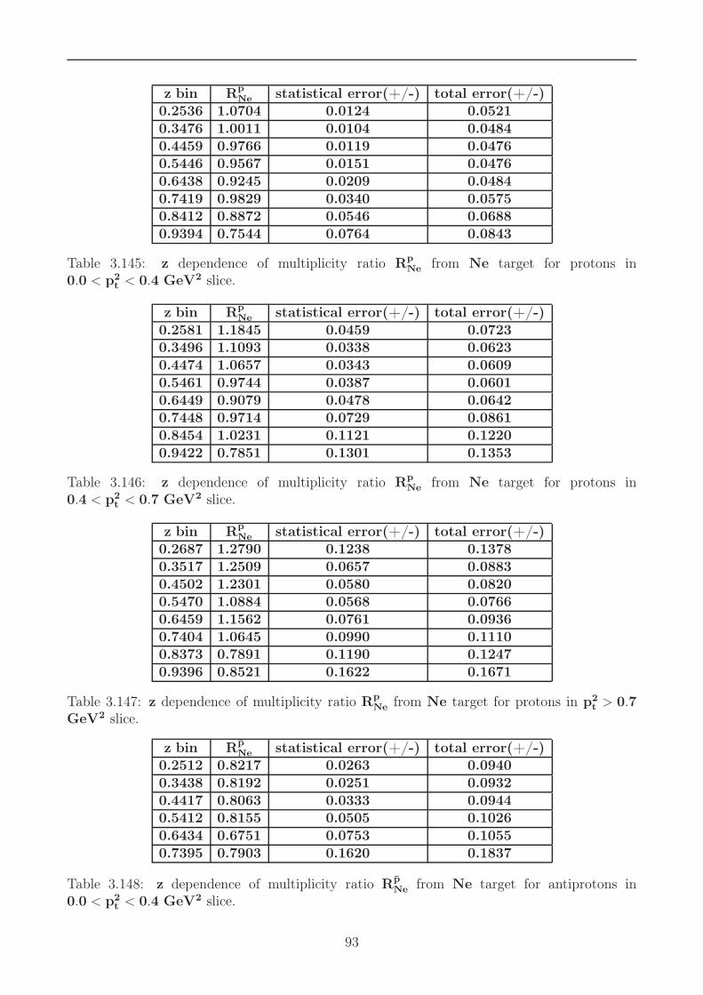
z bin Rp
Ne statistical error(+/-) total error(+/-)0.2536 1.0704 0.0124 0.05210.3476 1.0011 0.0104 0.04840.4459 0.9766 0.0119 0.04760.5446 0.9567 0.0151 0.04760.6438 0.9245 0.0209 0.04840.7419 0.9829 0.0340 0.05750.8412 0.8872 0.0546 0.06880.9394 0.7544 0.0764 0.0843
Table 3.145: z dependence of multiplicity ratio Rp
Ne from Ne target for protons in0.0 < p2
t < 0.4 GeV2 slice.
z bin RpNe statistical error(+/-) total error(+/-)
0.2581 1.1845 0.0459 0.07230.3496 1.1093 0.0338 0.06230.4474 1.0657 0.0343 0.06090.5461 0.9744 0.0387 0.06010.6449 0.9079 0.0478 0.06420.7448 0.9714 0.0729 0.08610.8454 1.0231 0.1121 0.12200.9422 0.7851 0.1301 0.1353
Table 3.146: z dependence of multiplicity ratio RpNe from Ne target for protons in
0.4 < p2t < 0.7 GeV2 slice.
z bin Rp
Ne statistical error(+/-) total error(+/-)0.2687 1.2790 0.1238 0.13780.3517 1.2509 0.0657 0.08830.4502 1.2301 0.0580 0.08200.5470 1.0884 0.0568 0.07660.6459 1.1562 0.0761 0.09360.7404 1.0645 0.0990 0.11100.8373 0.7891 0.1190 0.12470.9396 0.8521 0.1622 0.1671
Table 3.147: z dependence of multiplicity ratio RpNe from Ne target for protons in p2
t > 0.7GeV2 slice.
z bin Rp̄
Ne statistical error(+/-) total error(+/-)0.2512 0.8217 0.0263 0.09400.3438 0.8192 0.0251 0.09320.4417 0.8063 0.0333 0.09440.5412 0.8155 0.0505 0.10260.6434 0.6751 0.0753 0.10550.7395 0.7903 0.1620 0.1837
Table 3.148: z dependence of multiplicity ratio Rp̄Ne from Ne target for antiprotons in
0.0 < p2t < 0.4 GeV2 slice.
93

z bin Rp̄Ne statistical error(+/-) total error(+/-)
0.2582 0.7611 0.0695 0.10860.3473 0.8070 0.0653 0.10990.4452 0.7635 0.0753 0.11250.5395 0.8506 0.1231 0.15440.6362 0.7918 0.1773 0.1974
Table 3.149: z dependence of multiplicity ratio Rp̄
Ne from Ne target for antiprotons in0.4 < p2
t < 0.7 GeV2 slice.
z bin Rp̄
Ne statistical error(+/-) total error(+/-)0.2685 0.9993 0.1991 0.22720.3515 0.7429 0.0976 0.12710.4440 1.1716 0.1600 0.20510.5442 1.0635 0.2203 0.24920.6370 1.1993 0.4091 0.4299
Table 3.150: z dependence of multiplicity ratio Rp̄Ne from Ne target for antiprotons p2
t > 0.7GeV2 slice.
z bin Rπ+
Kr statistical error(+/-) total error(+/-)0.0940 0.9538 0.0330 0.04780.1558 0.8569 0.0039 0.03210.2462 0.7939 0.0034 0.03000.3454 0.7583 0.0042 0.02780.4459 0.7319 0.0052 0.02610.5465 0.7184 0.0065 0.02480.6467 0.7087 0.0079 0.02530.7465 0.6776 0.0092 0.02590.8462 0.6279 0.0105 0.03250.9394 0.5494 0.0117 0.0265
Table 3.151: z dependence of multiplicity ratio Rπ+
Kr from Kr target for positively charged pionsin 0.0 < p2
t < 0.4 GeV2 slice.
94

z bin Rπ+
Kr statistical error(+/-) total error(+/-)0.1805 0.9929 0.0491 0.06140.2542 0.9459 0.0166 0.03920.3479 0.8517 0.0135 0.03370.4459 0.7872 0.0147 0.03120.5456 0.7401 0.0170 0.02990.6461 0.7296 0.0202 0.03190.7460 0.6181 0.0225 0.03160.8429 0.5993 0.0287 0.04100.9364 0.5057 0.0338 0.0402
Table 3.152: z dependence of multiplicity ratio Rπ+
Kr from Kr target for positively charged pionsin 0.4 < p2
t < 0.7 GeV2 slice.
z bin Rπ+
Kr statistical error(+/-) total error(+/-)0.2652 1.0787 0.0513 0.06540.3531 1.0001 0.0285 0.04610.4501 0.9514 0.0248 0.04150.5480 0.8719 0.0247 0.03810.6446 0.7742 0.0263 0.03710.7440 0.6778 0.0303 0.03880.8433 0.6200 0.0394 0.04970.9351 0.6258 0.0525 0.0591
Table 3.153: z dependence of multiplicity ratio Rπ+
Kr from Kr target for positively charged pionsin p2
t > 0.7 GeV2 slice.
z bin Rπ−
Kr statistical error(+/-) total error(+/-)0.0941 0.9187 0.0332 0.05220.1552 0.8448 0.0041 0.03970.2458 0.7892 0.0037 0.03820.3452 0.7501 0.0046 0.03220.4456 0.7207 0.0058 0.02780.5459 0.7205 0.0073 0.02680.6472 0.7091 0.0089 0.02820.7468 0.6867 0.0106 0.03220.8457 0.6734 0.0124 0.05210.9401 0.5730 0.0137 0.0376
Table 3.154: z dependence of multiplicity ratio Rπ−
Kr from Kr target for negatively chargedpions in 0.0 < p2
t < 0.4 GeV2 slice.
95
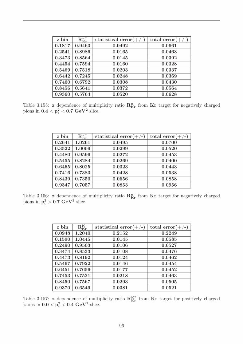
z bin Rπ−
Kr statistical error(+/-) total error(+/-)0.1817 0.9463 0.0492 0.06610.2541 0.8986 0.0165 0.04630.3473 0.8564 0.0145 0.03920.4454 0.7594 0.0160 0.03280.5469 0.7518 0.0203 0.03370.6442 0.7245 0.0248 0.03690.7460 0.6792 0.0308 0.04300.8456 0.5641 0.0372 0.05640.9360 0.5764 0.0520 0.0628
Table 3.155: z dependence of multiplicity ratio Rπ−
Kr from Kr target for negatively chargedpions in 0.4 < p2
t < 0.7 GeV2 slice.
z bin Rπ−
Kr statistical error(+/-) total error(+/-)0.2641 1.0261 0.0495 0.07000.3522 1.0009 0.0299 0.05200.4480 0.9596 0.0272 0.04530.5455 0.8284 0.0269 0.04000.6465 0.8025 0.0323 0.04430.7416 0.7383 0.0428 0.05380.8439 0.7350 0.0656 0.08580.9347 0.7057 0.0853 0.0956
Table 3.156: z dependence of multiplicity ratio Rπ−
Kr from Kr target for negatively chargedpions in p2
t > 0.7 GeV2 slice.
z bin RK+
Kr statistical error(+/-) total error(+/-)0.0948 1.2040 0.2152 0.22490.1590 1.0445 0.0145 0.05850.2490 0.9503 0.0106 0.05270.3474 0.8533 0.0108 0.04760.4473 0.8192 0.0124 0.04620.5467 0.7922 0.0146 0.04540.6451 0.7656 0.0177 0.04520.7453 0.7521 0.0218 0.04630.8450 0.7567 0.0293 0.05050.9370 0.6549 0.0381 0.0521
Table 3.157: z dependence of multiplicity ratio RK+
Kr from Kr target for positively chargedkaons in 0.0 < p2
t < 0.4 GeV2 slice.
96

z bin RK+
Kr statistical error(+/-) total error(+/-)0.1828 1.1262 0.1369 0.15000.2558 1.1302 0.0456 0.07650.3497 1.0088 0.0344 0.06470.4480 0.8969 0.0330 0.05880.5456 0.8560 0.0360 0.05880.6460 0.8246 0.0411 0.06080.7431 0.6691 0.0426 0.05600.8445 0.6566 0.0559 0.06630.9332 0.6498 0.0826 0.0898
Table 3.158: z dependence of multiplicity ratio RK+
Kr from Kr target for positively chargedkaons in 0.4 < p2
t < 0.7 GeV2 slice.
z bin RK+
Kr statistical error(+/-) total error(+/-)0.2672 1.2579 0.1207 0.13870.3542 1.2545 0.0701 0.09780.4493 1.0687 0.0521 0.07800.5474 1.0190 0.0505 0.07490.6453 0.8587 0.0478 0.06680.7436 0.8545 0.0599 0.07580.8436 0.6871 0.0770 0.08560.9372 0.5899 0.1048 0.1096
Table 3.159: z dependence of multiplicity ratio RK+
Kr from Kr target for positively chargedkaons in p2
t > 0.7 GeV2 slice.
z bin RK−
Kr statistical error(+/-) total error(+/-)0.0950 0.7225 0.1796 0.18380.1586 0.8900 0.0158 0.05090.2471 0.8240 0.0130 0.04660.3453 0.7478 0.0145 0.04310.4458 0.7555 0.0187 0.04510.5443 0.6775 0.0220 0.04290.6433 0.6807 0.0319 0.04880.7409 0.6288 0.0452 0.05670.8410 0.7239 0.0840 0.09280.9373 0.4830 0.1441 0.1466
Table 3.160: z dependence of multiplicity ratio RK−
Kr from Kr target for negatively chargedkaons in 0.0 < p2
t < 0.4 GeV2 slice.
97

z bin RK−
Kr statistical error(+/-) total error(+/-)0.1822 1.0073 0.1685 0.17720.2555 0.8687 0.0469 0.06650.3478 0.9263 0.0444 0.06710.4460 0.7776 0.0484 0.06420.5459 0.7547 0.0592 0.07200.6425 0.6897 0.0753 0.08410.7506 0.5701 0.0964 0.10130.8412 0.5085 0.1632 0.16550.9300 0.0815 0.1183 0.1184
Table 3.161: z dependence of multiplicity ratio RK−
Kr from Kr target for negatively chargedkaons in 0.4 < p2
t < 0.7 GeV2 slice.
z bin RK−
Kr statistical error(+/-) total error(+/-)0.2673 1.1766 0.1434 0.15700.3526 0.8437 0.0681 0.08210.4493 0.8831 0.0679 0.08310.5459 0.8454 0.0766 0.08930.6424 0.9070 0.1025 0.11370.7394 0.8824 0.1711 0.17770.8492 0.4470 0.2123 0.2137
Table 3.162: z dependence of multiplicity ratio RK−
Kr from Kr target for negatively chargedkaons in p2
t > 0.7 GeV2 slice.
z bin Rp
Kr statistical error(+/-) total error(+/-)0.2523 1.2067 0.0121 0.05860.3467 0.9977 0.0096 0.04800.4448 0.8821 0.0104 0.04290.5444 0.8032 0.0126 0.03990.6431 0.7589 0.0174 0.03980.7430 0.7520 0.0265 0.04430.8418 0.6852 0.0431 0.05390.9413 0.6601 0.0622 0.0696
Table 3.163: z dependence of multiplicity ratio Rp
Kr from Kr target for protons in0.0 < p2
t < 0.4 GeV2 slice.
98

z bin RpKr statistical error(+/-) total error(+/-)
0.2581 1.4881 0.0495 0.08590.3489 1.3229 0.0349 0.07150.4461 1.1054 0.0323 0.06130.5457 0.9272 0.0348 0.05590.6462 0.8082 0.0415 0.05640.7441 0.7580 0.0569 0.06720.8482 0.6030 0.0713 0.07680.9427 0.6234 0.1043 0.1084
Table 3.164: z dependence of multiplicity ratio Rp
Kr from Kr target for protons in0.4 < p2
t < 0.7 GeV2 slice.
z bin RpKr statistical error(+/-) total error(+/-)
0.2692 1.6904 0.1382 0.15950.3524 1.6629 0.0719 0.10640.4489 1.6580 0.0655 0.10200.5478 1.3331 0.0600 0.08690.6444 1.1698 0.0694 0.08870.7451 0.9432 0.0825 0.09370.8380 1.0016 0.1367 0.14460.9479 1.0315 0.1659 0.1729
Table 3.165: z dependence of multiplicity ratio Rp
Kr from Kr target for protons in p2t > 0.7
GeV2 slice.
z bin Rp̄
Kr statistical error(+/-) total error(+/-)0.2493 0.7647 0.0214 0.08650.3430 0.7019 0.0200 0.07940.4418 0.6336 0.0258 0.07400.5430 0.6706 0.0406 0.08390.6416 0.6712 0.0685 0.10050.7335 0.4720 0.1197 0.1305
Table 3.166: z dependence of multiplicity ratio Rp̄Kr from Kr target for antiprotons in
0.0 < p2t < 0.4 GeV2 slice.
z bin Rp̄
Kr statistical error(+/-) total error(+/-)0.2557 0.8528 0.0743 0.11940.3434 0.7243 0.0575 0.09800.4459 0.7927 0.0744 0.11440.5479 0.5367 0.0810 0.10010.6460 0.4450 0.1211 0.1306
Table 3.167: z dependence of multiplicity ratio Rp̄Kr from Kr target for antiprotons in
0.4 < p2t < 0.7 GeV2 slice.
99

z bin Rp̄Kr statistical error(+/-) total error(+/-)
0.2649 1.1137 0.2364 0.26610.3499 0.9020 0.1106 0.14830.4455 0.6695 0.0956 0.12050.5455 0.9534 0.1621 0.19290.6382 0.5777 0.1725 0.1837
Table 3.168: z dependence of multiplicity ratio Rp̄
Kr from Kr target for antiprotons in p2t > 0.7
GeV2 slice.
z bin Rπ+
Xe statistical error(+/-) total error(+/-)0.0940 0.9073 0.0386 0.05130.1558 0.8245 0.0045 0.03150.2461 0.7417 0.0040 0.02950.3456 0.7002 0.0047 0.02650.4455 0.6719 0.0059 0.02420.5465 0.6583 0.0073 0.02310.6465 0.6362 0.0088 0.02330.7460 0.6229 0.0104 0.02460.8457 0.5751 0.0119 0.03180.9403 0.4765 0.0129 0.0251
Table 3.169: z dependence of multiplicity ratio Rπ+
Xe from Xe target for positively charged pionsin 0.0 < p2
t < 0.4 GeV2 slice.
z bin Rπ+
Xe statistical error(+/-) total error(+/-)0.1804 1.0593 0.0610 0.07290.2546 0.9270 0.0195 0.04140.3486 0.7967 0.0153 0.03340.4457 0.7408 0.0169 0.03090.5459 0.6681 0.0191 0.02930.6468 0.6266 0.0219 0.03050.7460 0.5832 0.0258 0.03320.8442 0.5250 0.0315 0.04140.9404 0.5027 0.0403 0.0463
Table 3.170: z dependence of multiplicity ratio Rπ+
Xe from Xe target for positively charged pionsin 0.4 < p2
t < 0.7 GeV2 slice.
100

z bin Rπ+
Xe statistical error(+/-) total error(+/-)0.2652 1.0614 0.0596 0.07280.3522 1.0244 0.0344 0.05140.4490 0.8953 0.0283 0.04220.5472 0.8505 0.0288 0.04040.6456 0.7573 0.0311 0.04030.7431 0.6693 0.0356 0.04290.8390 0.5238 0.0426 0.05030.9408 0.5810 0.0599 0.0654
Table 3.171: z dependence of multiplicity ratio Rπ+
Xe from Xe target for positively charged pionsin p2
t > 0.7 GeV2 slice.
z bin Rπ−
Xe statistical error(+/-) total error(+/-)0.0941 0.8972 0.0391 0.05680.1551 0.8246 0.0048 0.04000.2457 0.7421 0.0043 0.03770.3449 0.6961 0.0052 0.03100.4457 0.6639 0.0066 0.02630.5460 0.6755 0.0084 0.02680.6458 0.6499 0.0101 0.02720.7459 0.6232 0.0119 0.03230.8472 0.6029 0.0139 0.05110.9400 0.5421 0.0159 0.0388
Table 3.172: z dependence of multiplicity ratio Rπ−
Xe from Xe target for negatively chargedpions in 0.0 < p2
t < 0.4 GeV2 slice.
z bin Rπ−
Xe statistical error(+/-) total error(+/-)0.1803 0.9904 0.0596 0.07640.2538 0.8849 0.0193 0.04860.3468 0.8037 0.0166 0.03900.4460 0.7809 0.0195 0.03570.5436 0.6975 0.0232 0.03510.6449 0.6567 0.0278 0.03770.7440 0.6350 0.0353 0.04670.8418 0.6067 0.0466 0.06800.9372 0.5585 0.0612 0.0713
Table 3.173: z dependence of multiplicity ratio Rπ−
Xe from Xe target for negatively chargedpions in 0.4 < p2
t < 0.7 GeV2 slice.
101

z bin Rπ−
Xe statistical error(+/-) total error(+/-)0.2640 1.1100 0.0624 0.08390.3515 1.0089 0.0352 0.05660.4495 0.9583 0.0322 0.04880.5463 0.8154 0.0315 0.04400.6460 0.7867 0.0382 0.04890.7425 0.6525 0.0473 0.05680.8433 0.5874 0.0679 0.08310.9295 0.6569 0.0956 0.1048
Table 3.174: z dependence of multiplicity ratio Rπ−
Xe from Xe target for negatively chargedpions in p2
t > 0.7 GeV2 slice.
z bin RK+
Xe statistical error(+/-) total error(+/-)0.0946 1.0747 0.2391 0.24610.1592 1.0267 0.0167 0.05820.2489 0.8978 0.0123 0.05030.3474 0.8018 0.0124 0.04530.4467 0.7590 0.0141 0.04360.5465 0.7527 0.0169 0.04420.6458 0.7391 0.0209 0.04530.7452 0.7108 0.0252 0.04610.8426 0.6680 0.0323 0.04860.9372 0.5996 0.0427 0.0537
Table 3.175: z dependence of multiplicity ratio RK+
Xe from Xe target for positively chargedkaons in 0.0 < p2
t < 0.4 GeV2 slice.
z bin RK+
Xe statistical error(+/-) total error(+/-)0.1822 1.3107 0.1855 1.19870.2556 1.2877 0.0597 0.09190.3502 1.0205 0.0412 0.06910.4470 0.8484 0.0382 0.05990.5466 0.8041 0.0411 0.06000.6452 0.8200 0.0483 0.06570.7448 0.6402 0.0498 0.06070.8399 0.6321 0.0660 0.07440.9385 0.6524 0.0971 0.1034
Table 3.176: z dependence of multiplicity ratio RK+
Xe from Xe target for positively chargedkaons in 0.4 < p2
t < 0.7 GeV2 slice.
102
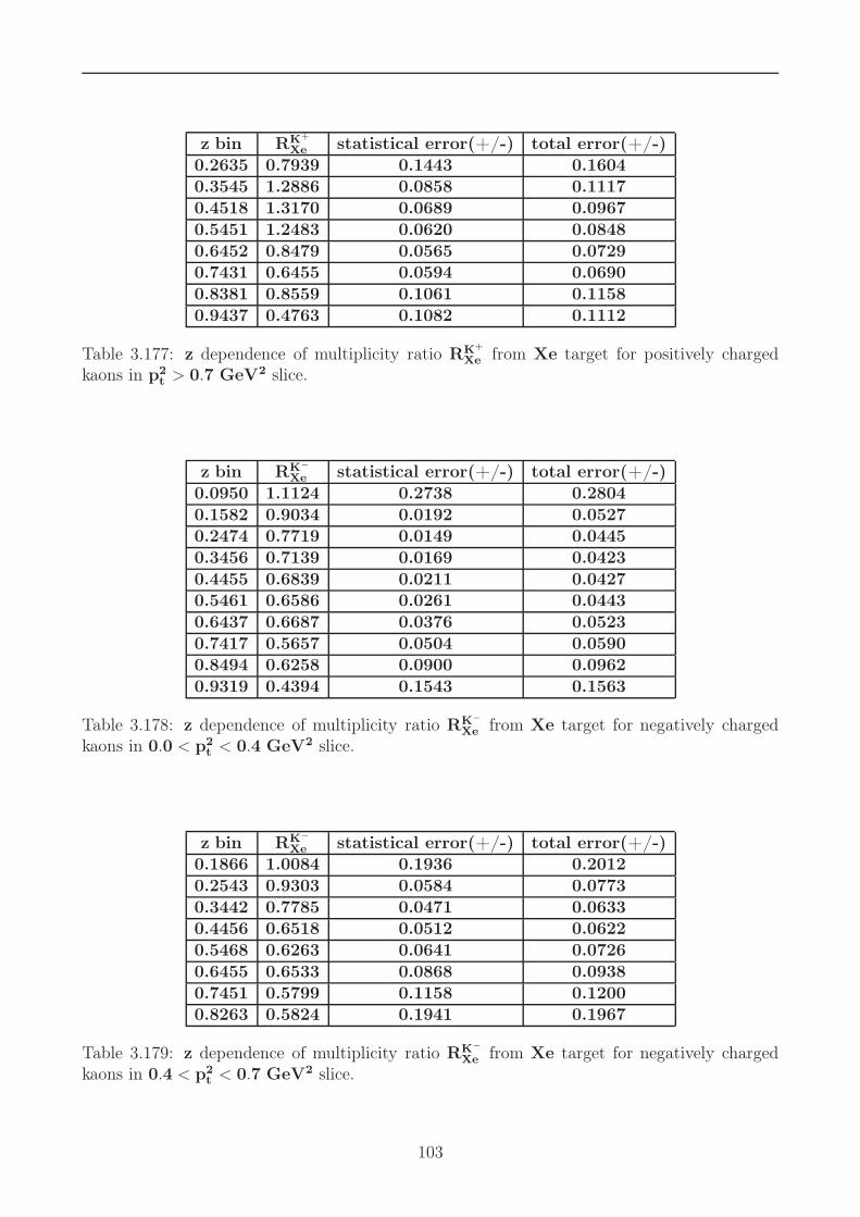
z bin RK+
Xe statistical error(+/-) total error(+/-)0.2635 0.7939 0.1443 0.16040.3545 1.2886 0.0858 0.11170.4518 1.3170 0.0689 0.09670.5451 1.2483 0.0620 0.08480.6452 0.8479 0.0565 0.07290.7431 0.6455 0.0594 0.06900.8381 0.8559 0.1061 0.11580.9437 0.4763 0.1082 0.1112
Table 3.177: z dependence of multiplicity ratio RK+
Xe from Xe target for positively chargedkaons in p2
t > 0.7 GeV2 slice.
z bin RK−
Xe statistical error(+/-) total error(+/-)0.0950 1.1124 0.2738 0.28040.1582 0.9034 0.0192 0.05270.2474 0.7719 0.0149 0.04450.3456 0.7139 0.0169 0.04230.4455 0.6839 0.0211 0.04270.5461 0.6586 0.0261 0.04430.6437 0.6687 0.0376 0.05230.7417 0.5657 0.0504 0.05900.8494 0.6258 0.0900 0.09620.9319 0.4394 0.1543 0.1563
Table 3.178: z dependence of multiplicity ratio RK−
Xe from Xe target for negatively chargedkaons in 0.0 < p2
t < 0.4 GeV2 slice.
z bin RK−
Xe statistical error(+/-) total error(+/-)0.1866 1.0084 0.1936 0.20120.2543 0.9303 0.0584 0.07730.3442 0.7785 0.0471 0.06330.4456 0.6518 0.0512 0.06220.5468 0.6263 0.0641 0.07260.6455 0.6533 0.0868 0.09380.7451 0.5799 0.1158 0.12000.8263 0.5824 0.1941 0.1967
Table 3.179: z dependence of multiplicity ratio RK−
Xe from Xe target for negatively chargedkaons in 0.4 < p2
t < 0.7 GeV2 slice.
103

z bin RK−
Xe statistical error(+/-) total error(+/-)0.2637 1.1789 0.1743 0.18570.3525 0.9233 0.0867 0.10020.4497 0.8328 0.0779 0.09010.5461 0.9047 0.0957 0.10760.6375 0.7190 0.1078 0.11470.7507 1.0880 0.2379 0.24510.8256 1.2152 0.4661 0.4708
Table 3.180: z dependence of multiplicity ratio RK−
Xe from Xe target for negatively chargedkaons in p2
t > 0.7 GeV2 slice.
z bin Rp
Xe statistical error(+/-) total error(+/-)0.2525 1.2323 0.0144 0.06050.3466 0.9735 0.0112 0.04730.4451 0.8533 0.0121 0.04210.5441 0.7718 0.0146 0.03920.6431 0.6889 0.0195 0.03790.7421 0.6505 0.0288 0.04210.8407 0.7152 0.0523 0.06220.9421 0.5071 0.0637 0.0680
Table 3.181: z dependence of multiplicity ratio RpXe from Xe target for protons in
0.0 < p2t < 0.4 GeV2 slice.
z bin RpXe statistical error(+/-) total error(+/-)
0.2579 1.5092 0.0580 0.09180.3484 1.3602 0.0419 0.07660.4449 1.0603 0.0372 0.06230.5456 0.8780 0.0393 0.05710.6442 0.7943 0.0487 0.06140.7446 0.6761 0.0634 0.07100.8437 0.6765 0.0902 0.09570.9443 0.4832 0.1044 0.1069
Table 3.182: z dependence of multiplicity ratio RpXe from Xe target for protons in
0.4 < p2t < 0.7 GeV2 slice.
104

z bin Rp
Xe statistical error(+/-) total error(+/-)0.2689 2.2011 0.1902 0.21670.3511 1.6757 0.0834 0.11490.4477 1.6727 0.0773 0.11050.5453 1.2491 0.0681 0.09010.6420 1.0608 0.0763 0.09130.7436 0.9320 0.0986 0.10800.8431 1.0264 0.1694 0.17620.9408 0.8090 0.1700 0.1742
Table 3.183: z dependence of multiplicity ratio Rp
Xe from Xe target for protons in p2t > 0.7
GeV2 slice.
z bin Rp̄Xe statistical error(+/-) total error(+/-)
0.2497 0.7303 0.0239 0.08350.3428 0.6485 0.0224 0.07450.4437 0.5886 0.0290 0.07070.5430 0.5920 0.0445 0.07870.6393 0.4834 0.0671 0.08550.7344 0.3929 0.1224 0.1298
Table 3.184: z dependence of multiplicity ratio Rp̄
Xe from Xe target for antiprotons in0.0 < p2
t < 0.4 GeV2 slice.
z bin Rp̄
Xe statistical error(+/-) total error(+/-)0.2565 0.7949 0.0863 0.12260.3497 0.7657 0.0694 0.10890.4463 0.7416 0.0880 0.11980.5378 0.7059 0.1136 0.13740.6358 0.7970 0.2011 0.2193
Table 3.185: z dependence of multiplicity ratio Rp̄Xe from Xe target for antiprotons in
0.4 < p2t < 0.7 GeV2 slice.
105

z bin Rp̄Xe statistical error(+/-) total error(+/-)
0.2614 1.0839 0.2661 0.29140.3493 1.0229 0.1395 0.17900.4429 0.7270 0.1227 0.14630.5468 0.9633 0.1974 0.22390.6437 0.8221 0.2474 0.2633
Table 3.186: z dependence of multiplicity ratio Rp̄
Xe from Xe target for antiprotons in p2t > 0.7
GeV2 slice.
3.5 Conclusion
The first multidimensional kinematic dependencies of hadron multiplicity ratio RhA have
been extracted for pions(π+, π−), kaons(K+, K−) and protons(p, p̄) on neon, krypton and
xenon targets relative to deuterium. The raw hadron yields are corrected from RICH misiden-
tification effects which are found to be essential for protons and kaons and practically not
relevant for pions. Using the corrected hadron yields the multidimensional nuclear attenuation
effect is considered. For π+ and π− the behaviour of RhA was about the same within the exper-
imental uncertainties. The dependence of RK+
A on ν for positevely charged kaons was found to
be different from Rπ+
A , Rπ−
A and RK−
A at high values of z which might be the result of different
modification of fragmentation functions in nuclear medium. Proton data show a significant
difference from the other hadrons which can be explained by a contribution of knock-out pro-
cesses, in addition to the fragmentation process. The idea is that apart from fragmentation
process some protons might be knock-outed from nuclei due to the final state interaction. The
expected spectrum for these protons should lie at small momentum range which reflected in
data by the smallest z slice.
Looking on z dependence of RhA in three slices of ν we have found that the attenuation
is small for positively charged kaons than it is for negatively charged ones. This phenomena
might be a reflection of transformation of proton into a (K+Λ) pair inside a nucleus which is
suppressed for negatively charged kaons due to the quark content. We also see that the Cronin
effect is suppressed at large values of z. A possible explanation based on the phenomenology
approach is that at high z values the production time is very small thus the contribution
106

from partonic effects is highly suppressed. On the other hand, it is assumed that the main
contribution into transverse momentum broadening comes from the partonic effects.
The hadron multiplicity ratio also depends on azimuthal angle φ but our experimental
data show no φ dependence within the experimental uncertainties. It is also important to
mention almost no Q2 dependence for the nuclear attenuation. Because in the HERMES
kinematics Q2 and xBj are strongly correlated the same is true for xBj dependences.
Having the first multidimensional data of the nuclear attenuation for charged pions, kaons
and proton-antiprotons from neon, krypton and xenon targets, it is important to check different
models which based on the one-dimensional approach and make a new predictions for hadroniza-
tion process in nuclear medium. These new more detailed data provide a great opportunity for
such a test of various model predictions in wide kinematic regime.
107

Acknowledgements
I would like to express my thanks of gratitude to the HERMES Yerevan groupe,
specially the group leader and my scientific supervisor professor Norik Akopov for
the excelent opportunity to deal with the excelent data provided by the HERMES
experiment. It has been really amazing and I was enjoyed almost every day dealing
with these small guys : hadrons, which sometimes were insufferable(there is a one
named pi0).
Thanks to all of you R. Avakian A. Avetisyan, L. Grigoryan, G. Elbakyan, H.
Marukyan, Z. Akopov, A. Movsisyan and A. Petrosyan for your help and support
during these years.
I am very appreciative of the HERMES management Klaus Rith, Gunar Schnell,
Marco Contalbrigo, Ami Rostomyan for supporting my attendence to various con-
ferences where I’ve learned many things and found to me that not everithing is
written in textbooks, although I was not so naive...
I would like to thank to Achim Hillenbrand and Sylvester Joosten, I’ve worked with
on the nice topic called multiplicity.
I also sincerely appreciate Hamlet Mkrtchyan and Jora Arakelyan for their proof-
reading and constructive remarks of the thesis. Many thanks to Mareta Hakobyan
for her huge support to complete the official part of this thesis which I would never
did myself.
Last but not least, I greatly appreciate my family for their patience and love during
all this time.

References
[1]. John C. Collins et al., Factorization for hard exclusive electroproduction of
mesons in QCD, Phys. Rev. D 56, 2982âĂŞ3006 (1997). 5
[2]. John C. Collins, Universality of soft and collinear factors in hard scattering
factorization, Phys.Rev.Lett. 93 (2004) 252001. 6
[3]. L. Osborne et al., Electroproduction of hadrons from nuclei, Phys.Rev.Lett. 40
(1978) 1624. 6
[4]. J. Ashman et al., Comparison of forward hadrons produced in muon inter-
actions on nuclear targets and deuterium, [EMC] Z. Phys. C52 (1991) 1. 6, 8,
41
[5]. A. Airapetian et al., Hadronization in Semi-inclusive deep inelastic scattering
on nuclei, Nucl. Phys. B 780 (2007) 1-27. 6, 41
[6]. W.K. Brooks et al., Studies of parton propogation and hadron formation in the
space-time domain, AIP Conf.Proc. 1056 (2008) 215-222. 6
[7]. L. Grigoryan (Yerevan Phys. Inst.), Study of the multiplicity of hadrons on
nuclei., Armenian J.Phys. 5 (2012) 95-100. 6
[8]. B. Andersson et al., Parton fragmentation and string dynamics, Phys.Rept. 97
(1983) 31-45. 7, 34
[9]. A. Airapetian et al., Hadron formation in deep-inelastic positron scattering
from 14N and 2H , Eur. Phys. J. C 20 (2001) 479-486. 7
109
REFERENCES
[10]. N. Akopov, L. Grigoryan, Z. Akopov, Study of the hadronization process in
cold nuclear medium, Eur.Phys.J C(2010) 70 5-14. 8
[11]. B. Kopeliovich, J. Nemchik, E. Predazzi, Nuclear hadronization : Within or
without?, Nucl.Phys. A740 (2004) 211-245. 11, 78
[12]. A. Accardi, V. Muccifora, H.J. Pirner, Hadron production in deep inelastic
lepton nucleuse scattering, Nucl.Phys. A720 (2003) 131-156. 13
[13]. T. Falter, W. Cassing, K. Gallmaiser, U. Mosel, Hadron formation and
attenuation in deep inelastic lepton scattering off nuclei, Phys.Lett. B594 (2004)
61-68. 14
[14]. HERMES Collaboration, A. Airapetian et al., Nucl. Instrum. Meth. A540, 68
(2005), physics/0408137. 17
[15]. HERMES Collaboration, K. Ackerstaff et al., Nucl. Instrum. Meth. A417,
230 (1998), hep-ex/9806008. 17
[16]. M. G. Beuzekom, E. Garutti, D. Heesbeen, J. J. M. Steijger, and J. Visser,
First experience with the HERMES silicon detector, Nucl. Instrum. Meth. A461,
247 (2001). 19
[17]. J. T. Brack et al., The HERMES forward tracking chambers: Construction,
operation and aging effects, Nucl. Instrum. Meth. A469, 47 (2001). 19
[18]. A. Andreev et al., Multiwire proportional chambers in the HERMES experi-
ment, Nucl. Instrum. Meth. A465, 482 (2001). 19
[19]. S. Bernreuther et al., The HERMES back drift chambers, Nucl. Instrum.
Meth. A416, 45 (1998), hep-ex/9803005. 19
[20]. H. Avakian et al., Performance of the electromagnetic calorimeter of the
HERMES experiment, Nucl. Instrum. Meth. A417, 69 (1998), hep-ex/9810004.
21
110
REFERENCES
[21]. N. Akopov et al., The HERMES dual-radiator ring imaging Cherenkov detec-
tor, Nucl. Instrum. Meth. A479, 511 (2002), physics/0104033. 21
[22]. U. Elschenbroich, Analysis of luminosity monitor data for different years,
HERMES internal note 02-013. 24
[23]. Hrayr H. Matevosyan (Adelaide U.), Wolfgang Bentz (Tokai U., Hiratsuka),
Ian C. Cloet (Washington U., Seattle & Adelaide U.), Anthony W. Thomas (Ade-
laide U.). Nov 2011. 13 pp., Transverse momentum dependent fragmenatation
and quark distribution functions from the NJL-jet model, Analysis of luminosity
monitor data for different years, Phys.Rev. D85 (2012) 014021. 31
[24]. S.Mert Aybat (NIKHEF, Amsterdam & Vrije U., Amsterdam), Ted C. Rogers
(Vrije U., Amsterdam). Jan 2011. 22 pp., TMD parton distribution and frag-
mentation functions with QCD evolution., Phys.Rev. D83 (2011) 114042. 31
[25]. S.Mert Aybat (NIKHEF, Amsterdam), John C. Collins (Penn State U.),
Jian-Wei Qiu (Brookhaven & YITP, Stony Brook), Ted C. Rogers (Vrije U.,
Amsterdam & YITP, Stony Brook). Oct 2011. 16 pp., The QCD evolution of the
Sivers function, Phys.Rev. D85 (2012) 034043. 31
[26]. P. Schweitzer, T. Teckentrup and A. Metz, Intrinsic transverse parton mo-
menta in deeply inelastic reactions, Phys. Rev. D81, 094019 (2010). 31
[27]. ÌĹ M. Glück, E. Reya and A. Vogt, Dynamical parton distributions revisited,
Eur. Phys. J. C5, 461âĂŞ470 (1998). 34
[28]. A. D. Martin, R. G. Roberts, W. J. Stirling and R. S. Thorne, Parton dis-
tributions and the LHC: W and Z production, Eur. Phys. J. C14, 133âĂŞ145
(2000). 34
[29]. J. Pumplin et al., New generation of parton distributions with uncertainties
from global QCD analysis, JHEP 07, 012, 1âĂŞ47 (2002). 34
111

REFERENCES
[31]. T. Sjostrand, L. Lonnblad, S. Mrenna, and P. Skands, (2003), hep-
ph/0308153. 35
[30]. CERN Application Software Group. Geant , Detector Descriprion and Simu-
lation Tool. CERN Program Library Long Writeup, W5013, 1994. 35
[32]. L. Mankiewicz, A. Schäfer and M. Veltri, PEPSI: A Monte Carlo generator
for polarized leptoproduction, Comput. Phys. Commun. 71, 305âĂŞ318 (1992).
36
[33]. G. Ingelman, A. Edin and J. Rathsman, LEPTO 6.5 - A Monte Carlo Genera-
tor for Deep Inelastic Lepton-Nucleon Scattering, Comput. Phys. Commun.101,
108âĂŞ134 (1997). 36
[34]. A.C. Miller Applying radiative corrections to ratios of cross sections for Deeply
Inelastic Scattering, HERMES Internal Note. 37
[35]. A. Airapetian et al, Multidimensional study of hadronization in nuclei, Eur.
Phys. J. A 47 (2011) 113. 40
[36]. A. Accardi et al., Parton propagation and fragmentation in QCD matter, Riv.
Nuovo Cim. 32, 439 (2010). 41
[37]. J.W. Cronin, H. J. Frisch, M. J. Shochet, J. P. Boymond, R.Mermod, P.
A. Piroue and R. L. Sumner, Production of hadrons with large transverse mo-
mentum at 200-GeV, 300-GeV, and 400-GeV, Phys. Rev. D 11 (1975) 3105.
78
[38]. A. Airapetian et al., Transverse momentum broadening of hadrons produced
in semi-inclusive deep-inelastic scattering on nuclei, Phys. Lett. B 684 (2010)
114-118. 78
[39]. B.Z. Kopeliovich (Heidelberg, Max Planck Inst. & Regensburg U. & Dubna,
JINR), J. Nemchik (Kosice, IEF), A. Schafer (Regensburg U.), A.V. Tarasov
112

REFERENCES
(Heidelberg, Max Planck INst. & Regensburg U. & Dubna, JINR), Cronin effect
in hadron production off nuclei, Phys. Rev. Lett. 88, 232303 (2002). 78
[40]. Alberto Accardi, Cronin effect in proton-nucleus collisions: a survey of theo-
retical models, arXiv:hep-ph/0212148. 78
113