Agricultural Productivity Growth in Latin America and the Caribbean (LAC):

An Analysis of Climatic Effects, Convergence, and Catch-up

Michée A. Lachaud1 Boris E. Bravo-Ureta

2 Carlos E. Ludena

3

Abstract

This study estimates a Climate Adjusted Total Factor Productivity (CATFP) for agriculture in

Latin America and Caribbean (LAC) countries. Climatic variability is introduced in SPF models

by including average annual maximum temperature, precipitation and its monthly intra-year

standard deviations, and the number of rainy days. Climatic conditions have a negative impact

on production becoming stronger at the end of the 2000s compared to earlier periods. An Error

Correction Model is applied to investigate catch-up and convergence across LAC countries.

Argentina defines the frontier in LAC and CATFP convergence is found across all South

American countries, Costa Rica, Mexico, Barbados and The Bahamas. Using IPCC 2014

scenarios, the study shows climatic variability induces significant reductions in productivity over

the 2013-2040 period. Estimated productivity losses due to climatic variability range from USD

12.7 to 89.1 billion in the LAC region depending on the scenario and the discount rate.

JEL Code: D24, Q54, O47, E27.

Key Words: Agriculture, Total Factor Productivity, Climate Effects, Convergence, Forecasting,

Latin America, Caribbean.

1 Assistant Research Professor, Department of Agricultural and Resource Economics, University of Connecticut,

email: lachaud.michee.arnold@gmail.com, Corresponding author 2 Professor, Department of Agricultural and Resource Economics, University of Connecticut and Adjunct Professor,

University of Talca 3 Economist, Climate Change and Sustainability Division, Inter-American Development Bank

This paper was prepared under funding of the project “Agricultural Productivity Growth in Latin America and the

Caribbean” (RG-K1351) coordinated by César Falconi, Carlos Ludena and Pedro Martel of the IDB.

1

1. Introduction

Economists and policy makers have understood the importance of agriculture in the development

process for some time (e.g., Johnston & Mellor, 1961), while the 2007-2008 financial and

economic crises brought heightened attention to food security and food prices among other

factors. The social upheaval experienced in several countries where people took to the streets to

protest against escalating food prices (Diao et al., 2008), has highlighted the importance of

achieving food independence. Recent studies have shown that increasing agricultural

productivity is fundamental for long-term poverty alleviation and for overall economic growth

(e.g., World Bank, 2008).

Furthermore, agriculture plays an important role in overall economic growth in Latin

American and the Caribbean (LAC) countries (World Bank, 2003), and it has significant

spillover effects on other sectors of the economy (Hazell & Roell, 1983; Krueger et al., 1991;

Federico, 2005). According to the Economic Commission for Latin America and the Caribbean

(ECLAC, 2014), in 2012, the sector accounts for nearly 5% of Gross Domestic Product (GDP),

employs 16% of the workforce and produces about 23% of the total exports of the region.

Perry et al. (2005) have estimated that when accounting for the multiplier effect on other

sectors, agriculture’s share of Gross Domestic Product (GDP) in Latin America is about 50%

higher than what official statistical estimates indicate. Another reason to focus on agricultural

productivity among LAC countries, as pointed out by Chomitz and Buys (2007) and Stonich

(1989), among others, is the rising challenge imposed by climate change, natural resource

depletion and environmental degradation. According to the International Food Policy Research

Institute (IFPRI, 1995), approximately 200 million hectares of land in Latin America were

degraded during 1970-1995, and all the countries in the region, with the exception of Argentina,

had lost more than 5% of its forests. Moreover, since 1960, roughly 60% of forests in Central

America have been destroyed. More recent data from FAO (2010) reveals that South America

had the largest net loss of forests between 2000 and 2010 worldwide, which is estimated at 4.0

million hectares per year. Moreover, the forest cover continues to decrease in all countries in

Central America with the exception of Costa Rica. These data reveal that the expansion of the

2

agricultural frontier is still ongoing in several LAC countries, which can be a contributor to

climatic variability and thus can affect agricultural productivity (Geist & Lambin, 2000).

Most studies in agricultural productivity in the region are outdated and ignore unobserved

heterogeneity and climatic effects. The most recent published study is Ludena (2010), which is

based on data available up to 2007. Policy decisions made on outdated data can be misleading;

thus, agricultural productivity studies in the region need to be updated. One the other hand,

recent evidence from the fifth assessment report (AR5) of the Intergovernmental Panel on

Climate Change (IPCC) suggests that adverse impacts of climatic variability are more

pronounced in LAC than other regions of the world and are likely to be even worst in the future

(e.g., IPCC, 2014a; IPCC, 2014b; Stern, 2013). Specifically, climate projections indicate that

temperatures will rise by between 1.6 oC and 4

oC in the region by the end of the twenty-first

century while changes in precipitation levels are expected to range between -22% and 7% for

Central American countries; and, these changes would be more heterogeneous across South

American countries. Farming and livestock economic activities are responsive and vulnerable to

climatic variability and latest research findings highlight important prospective adverse impacts

on LAC agricultural sector by 2020 especially due to an increase in temperature levels and

changes in precipitation patterns (e.g., Vergara et al., 2013). Finally, while several studies (e.g.,

Mendelson & Dinar, 2003; Müller et al., 2010; Lobell et al., 2011; Ramirez et al., 2010) have

shown that agricultural productivity in Least Developing Countries (LDCs) is vulnerable to

climatic variability, few studies have focused on this topic in LAC. Therefore, a comprehensive

analysis of the relationship between agricultural productivity and climatic variability is critical

for LAC.

Several studies have examined agricultural productivity growth in LAC, some focusing

on specific countries (e.g., Bravo-Ureta & Cocchi, 2004; Gasques et al., 2012), others on several

LAC countries (e.g., Bharati & Fulginiti, 2007; Ludena et al., 2005), while yet others have

considered LAC along with countries from other parts of the globe (e.g., Bravo-Ortega &

Lederman, 2004; Coelli and Rao, 2005; Ludena, 2010). However, all these studies have

neglected the impact of climatic variability on agricultural productivity despite its potential

significance and implications regarding effective policy responses to sustain output growth.

3

There has been recently a growing body of literature that investigates the impact of

weather events such as temperature, precipitation, drought and so forth on economic outcomes.

First of all, it is worth noting that unlike weather that varies on a day-to-day basis and climate

change, which is a long-term gradual change in average weather conditions, climatic variability

can be seen as a yearly fluctuation in weather around a long-term average value.4 A better way to

look at it as explained by Dell et al. (2014) is that climate change can be interpreted as a

distribution in which climatic variability is a draw or a specific realization. This emerging

literature, based on panel data estimators, is motivated by the failure of cross sectional analysis

to establish a clear causative relationship between climate variables and economic output (Dell et

al., 2014). Therefore, this approach uses year-to-year variation to capture contemporaneous

effects of climate variables on economic outcomes. Specifically, it employs a reduced form panel

data approach, and has a causative interpretation that allows identifying, in our context, the net

effect of climatic variability on agricultural production and productivity (see Dell et al., 2014 for

an extensive review of the literature).

The objective of this study is to support the analysis of agricultural productivity growth

across LAC countries, with a special focus on the introduction of climate variables to produce

Climate Adjusted Total Factor Productivity Indexes (CATFP). This study will also provide a

comparative analysis of the convergence of TFP in agriculture within LAC countries, and

including forecasts to 2040 of possible productivity paths for LAC. In order to achieve that

objective, our conceptual framework and research methodology follows these steps: 1) Develop

a database that includes different types of climate variables, agricultural output, and conventional

inputs (tractors, fertilizer, animal stock, land and labor); 2) Use Stochastic Production Frontier

(SPF) methods along with panel data techniques to estimate alternative frontier models; compute

and decompose TFP into a Technical Efficiency (TE) index , Technological Progress (TP), a

Scale Efficiency (SE) index and Climate Effects (CE) which makes it possible to identify the

main drivers of productivity growth across countries; 3) Use panel data unit root co-integration

tests and the Error Correction Model (ECM) to analyze catch-up and convergence within LAC

countries and at the sub-regional level; 4) Forecast possible TFP paths for LAC countries to

2030-2040.

4 See http://www.climate.noaa.gov/education/pdfs/ClimateLiteracy-8.5x11March09FinalHR.pdf

4

The remainder of this paper is structured as follows: section two presents the analytical

framework; section three focuses on the data; section four presents the results; and section five is

devoted to the conclusion and a discussion of policy implications.

2. Analytical Framework

We investigate the impact of climatic variability on agricultural production and productivity by

using Stochastic Production Frontiers (SPF) and panel data techniques. The SPF method

basically estimates a benchmarking production frontier which serves to evaluate the performance

of each country in the sample. We estimate and test two sets of model specifications that vary

according to the treatment of the climatic variables and unobserved heterogeneity.

First, to account for country unobserved heterogeneity, such as unmeasured land quality

and environmental conditions that are not captured explicitly in the data and which potentially

affect the production, we estimate the Generalized True Random Effects (GTRE) model as

suggested by Colombi et al. (2011, 2014). A similar approach has also been presented recently

by Tsionas and Kumbhakar (2014), and Filippini and Greene (2014).

Second, the random effects specification assumes the absence of correlation between unit

specific effects and independent variables (Greene, 2008). However, if there is correlation

between unobserved heterogeneity and conventional inputs (e.g., land, labor, and machinery)

included in the production model and is ignored then the resulting estimates would be biased and

inconsistent. Therefore, we use the proposition of Farsi et al., (2005) and apply the Mundlak

(1978) adjustment to mitigate this problem and estimate what we call the Generalized True

Random Effects Mundlak (GTREM) model.

Both the GTRE and GTREM models are estimated by Simulated Maximum Likelihood

(SML). GRTE is an extension of the True Random Effects (TRE) proposed by Greene (2005a,

2005b). TRE models separate time variant inefficiency from time invariant country specific

unobserved heterogeneity. Consequently, TE estimates from TRE models offer information on

the time-varying component of inefficiency. Nevertheless, TRE models do not differentiate

unobserved country heterogeneity from time invariant inefficiency. Therefore, country time

invariant inefficiency and unobserved heterogeneity is captured as country random effects in the

TRE model.

5

The GTRE model proposed by Colombi et al., (2011, 2014) has an error term that is

decomposed into four elements and thus makes it possible to account separately for the usual

noise in the data, country unobserved time-invariant heterogeneity, time-varying or transient

inefficiency and time invariant or persistent inefficiency. Herein, the transient inefficiency is

interpreted as short-term TE (SRTE) associated with changes in managerial skills or disruptions

resulting from the adoption of new technologies. By contrast, persistent inefficiency can be seen

as long-run TE (LRTE) due to structural or institutional factors which evolve slowly overtime.

While LRTE and country unobserved heterogeneity are both time invariant effects, a major

difference between them is that the latter is considered to be not under the country decision

maker control (e.g., geological makeup of a country and other physical features or

characteristics). Unlike the three-step Tsionas and Kumbhakar (2014) estimator, and the Full

Information Maximum Likelihood (FIML) estimation proposed by Colombi (2011), we use a

recent one step estimator approach, based on simulation methods and on the Butler and Moffitt

(1982) formulation, suggested by Filippini and Greene (2014) who argue that it is more efficient

and unbiased.

We then use the estimated parameters from the GTRE SPF model to derive measures of

climatic impacts based on the methodology developed in Hughes et al., (2011). Subsequently, we

measure CATFP and decompose it into TE, TP, SE and CE using the approach suggested by

O’Donnell (2010, 2012), which satisfies basic axiomatic and economic properties. Finally, we

undertake a full analysis of CATFP.

2.1 Panel Data Stochastic Production Frontiers

There have been recent developments in panel data SPF analysis that make it possible to

separate country time invariant heterogeneity from time varying and time invariant inefficiencies

(e.g., Colombi et al., 2014). However, these new panel data SPF techniques have not been

exploited yet in most empirical work. In this section, we present the basic model specifications

that incorporate these new techniques.

We start with the panel data GTRE frontier model suggested by Colombi et al. (2014),

and Tsionas and Kumbhakar (2014), which, using a balanced panel data set, is given by:

6

where denotes the natural logarithm (log) of output for the i-th country in the t-th time

period; is a (1K) vector of inputs expressed in logs; T a time trend; is a (K1) vector of

unknown parameters to be estimated; and represents the j-th climate variable for the i-th

country in the t-th time period. The term vit is a random error that is assumed to follow a normal

distribution with mean zero and constant variance (vit iid ; and uit is a non-negative

unobservable random error, which captures the inefficiency of the i-th country in period t. The

inefficiency error term is assumed to follow a half-normal distribution. The term

represents a country time invariant inefficiency component and it has a half normal distribution

with underlying variance ; and

is a country specific random constant that

captures the unobserved heterogeneity which is assumed to be uncorrelated with the covariates

(e.g., Wooldridge, 2002, p.252); and is a common country constant. The other Greek letters

are parameters to be estimated. There are NT observations (N countries for T years).

We use the Cobb-Douglas (CD) functional form to approximate the underlying

technology of the SPF model in equation (1). Thus, the estimated parameters can be interpreted

directly as partial elasticities of production. The CD functional form is chosen because it is

globally consistent with economic and index number theories(i.e., non-negativity, monotonicity

and homogeneity) for obtaining transitive TFP indexes which is in contrast with the more

flexible and popular Translog (O’Donnell, 2012; O’Donnell and Nguyen, 2012).5

Greene (2005a, 2005b) has shown that we cannot use the Maximum Likelihood

Estimator (MLE) for TRE models because there is no closed form of the integral of associated

log-likelihood function. By relaxing the assumption of normal distribution of the time-invariant

effect and assuming instead a skew normal distribution, Filippini and Greene (2014) show that,

as is the case with the TRE models, the GTRE specification can be estimated by a SML method,

which consists of maximizing the log-likelihood based on a simulated estimate of the density

5 We first estimate the models using a Translog functional form, but these models, as expected, fail to satisfy the non-negativity of partial elasticities of production with respect to the inputs at all points in the dataset.

ity

itu

7

function (Greene, 2001; Train, 2002). Specifically, we denote as the time invariant

effect that has a skew normal distribution with parameters

Following Bhat (2001) and Greene (2005b), we use random draws from Halton sequences as the

simulation method and exploit the Butler and Moffitt (1982) formulation to estimate the models.

Recall that the GTRE model is based on the assumption that the regressors are not

correlated with country specific effects. To account for this correlation, we use the Mundlak

adjustment specification, which is also estimated by SML. The Mundlak correction model first

defines an auxiliary regression to capture the correlation between the country specific effect and

the independent variables as follows:

where

and

represents the random variable that drives the random

parameter. Equation 2 can then be inserted in equation 1 to obtain the Mundlak corrected

GTREM model (GTREM):

Technical efficiency is computed through simulation using the LIMPEP package

software developed by Greene (2012) and are based on the Jondrow, Lovell, Materov, and

Schmidt (JLMS) estimator (Jondrow et al., 1982). More precisely, the transient efficiency value

is derived from the following expression:

=

(4)

where = , =

represents the signal-to-noise ratio that captures the weight of

inefficiency in the total error term, and are the standard deviations of the inefficiency term

and the statistical noise of the composite error respectively, and . The terms

and are the standard normal and conditional density functions respectively.

u v

8

Subsequently, we compute . Analogously, the persistent

inefficiency counterpart is derived as . Finally, following Kumbhakar et

al., (2014), we compute a total TE measure as:

In the empirical application, the dependent variable ( ) is the natural logarithm of

agricultural production, is a set of inputs which includes tractors (TR), fertilizers (FER),

animal stock (AS), land (LA) and labor (LB); the smooth time trend, T, captures technological

progress; comprise annual average maximum temperature, annual average precipitation,

annual average rainy days, and monthly intra-year standard deviations of maximum temperature,

precipitation and rainy days; and the Greek letters represent parameters to be estimated.

2.2 Climate Effects Index (CEI)

We initially compute the change in output attributed to the climatic variables , using

the estimated parameters of equation 3, which is the preferred model as explained below. Thus:

The next step is to derive and compute the climate effects index (CEI), which captures

the joint effects of climatic variables on production (Hughes et al. 2011).

The , is then used to investigate the impact of changes in

maximum temperature, and rainy day patterns on production across countries and over time. The

CEI is non-negative by construction and values less than 1 indicate a negative impact on

production, values greater than 1 imply positive effects, and values equal to 1 reveal no impact.

2.3 O’Donnell TFP decomposition

Following O’Donnell (2012), for each country in each group, we define TFP as the ratio

of aggregate output to aggregate input. More formally, TFP for country i in year t is

ity

9

where is an aggregate output, and is an aggregate input. The index

that compares TFP of country i in year t with TFP of country k in year s is

where and .

Given the assumption of the Cobb-Douglas technology, equation 1 can be re-written as:

The TFP index in equation 9 satisfies all the economically relevant axioms from index

number theory. The first right-hand term is a measure of scale efficiency change where r

captures returns to scale and the Greek parameters are coefficients to be estimated. The second

component on the right-hand side captures climatic effects and the third technological progress.

The last component measures the output-oriented technical efficiency change and it is derived

from equation 5 (Kumbhakar et al., 2014).

2.4 Catch-up and Convergence

Catch-up is typically used to denote movements towards a country’s own frontier

(Kumbhakar et al., 2005; Kumar and Russell, 2002). Recall that the inefficiency (or efficiency)

estimate from equation 5 measures the distance of a given country at a specific time with respect

to its frontier. Therefore, when catch-up takes place the term is shrinking overtime. In other

words, a country that is catching-up experiences a relative increase in TE over time. It should be

noted that the overall TE expression in equation 5 is used in the calculation of TE. We analyze

the catch-up process by studying the temporal behavior of TE across LAC countries relative to

their own frontiers. This exercise can be repeated for the other countries in the full sample.

Convergence, another issue of significance in the analysis of productivity across

countries, is a measure of how the production possibility frontiers of the least performing

countries are moving with respect to the frontier of the best performing ones (Barro, 1997;

10

Baumol, 1986; Solow, 1956). Therefore, we investigate how CATFP of low performing

countries in LAC evolves overtime relative to that of high performing ones in the region. In other

words, we are investigating convergence in terms of CATFP across LAC countries. In addition,

we examine whether CATFP across LAC countries is converging to that of Europe (average

TFP) by using Europe as the reference frontier. 6

Barro (1991), Baumol (1986), De Long (1988), and Mankiw et al., (1992) have provided

some of the most significant contributions to the empirical convergence literature. These authors

have interpreted a negative relationship between the initial level of income and growth rates as a

sign of convergence. That is, given “n” countries in a group with different initial CATFP levels,

if countries with lower initial CATFP grow faster than those with a higher one, least productive

countries are approaching the frontier of the better performers over a given time horizon. This

notion of convergence is known as -convergence.

A more robust approach to test the convergence hypothesis across countries is based on

panel data Unit Root and Co-integration tests. A time series with a convergent long-run trend

should be either stationary or co-integrated because it has a common stochastic drift (Hamilton,

1994). That is, the series depicts a similar long-run pattern and it does not scatter over time.

Some previous studies examine convergence either in terms of technical efficiency (e.g.,

Cornwell and Wächter, 1999; Ludena et al., 2007), income per capita, labor productivity or TFP

(e.g., Bernard and Jones, 1996; Rao and Coelli, 2004). Most of those papers, and others, have

used conventional time series unit root and co-integration techniques to study convergence.

Applying classical time series methods might lead to the wrong conclusion of the non-stationary

of a series because the analysis is not based on structural equations and does not account for the

cross-sectional dependence of the data (Westerlund, 2007). We apply panel data unit root tests,

which have been used in just a few productivity studies (e.g., Ball et al., 2004; Suhariyanto and

Thirtle, 2001; Ludena, 2010; Liu et al., 2011). In addition, we consider panel data co-integration

tests to explore the existence of a long-run uniform trend among CATFP estimates across LAC

countries. The application of this latter methodology has been even more limited in the

productivity literature.

6 Section 4.3 discusses why the United States was not included in the present analysis.

11

We first start by testing the presence of a unit root among CATFP estimates. The

presence of a unit root in the CATFP series suggests that it is non-stationary. Stationarity is

important for long-run dynamics because it implies that the mean and all auto-covariances of

CATFP are finite and do not change over time (Hamilton, 1994). Specifically, we consider the

following auto-regressive (AR) process:

where are parameters to be estimated, and is assumed to be white noise. Under the

null hypothesis that CATFP estimates contain a unit root, we perform the Im-Pesaran-Shin (IPS)

(2003) and Levil-Lin-Chu (LLC) (2002) tests. The LLC test assumes a common autoregressive

parameter in the panel, which means that it is not permissible for the CATFP estimates for some

countries to contain unit roots while others do not. LLC (2002) have argued that individual unit

root tests in time series analysis has limited power and instead have suggested a group unit root

tests. In addition, we perform the IPS test because it relaxes the assumption of the common

autoregressive coefficient of the LLC test. This IPS test allows for heterogeneity of the

autoregressive roots between cross sections. Both the LLC and IPS tests are based on a t-test and

Augmented Dickey-Fuller (ADF) regressions. Moreover, we conduct the Breitung (2000) panel

data unit root test. Breitung has argued that the LLC and IPS tests loose power when individual

specific trends are taken into consideration. This last test is performed to check the robustness of

the LLC and IPS results. One of the advantages of the Panel unit root tests used here is that they

account for both the time-series and cross-sectional dimensions of the data (Westerlund, 2007).

Another advantage of using panel data unit root tests is that the estimators are normally

distributed (Ball et al., 2004).

We next proceed to the analysis of co-integration tests for non-stationary series. A

stationary linear combination of two or more non-stationary CATFP series implies that they are

co-integrated (Hamilton, 1994). As in the case of panel-data unit root tests, we use panel-data co-

integration tests that are arguably more powerful than those of the conventional time series

method based on the residuals because they do not entail the ad hoc assumption of cross-

sectional dependence, which requires that time series are independent across units, and do not

impose the common-factor restriction for long-run and short-run parameters (e.g., Banerjee et al.,

1998; Kremers et al., 1992).

12

We use the error-correction co-integration tests for panel data recently developed by

Westerlund (2007) and applied in recent empirical studies (e.g., Rassenfosse and Potterie, 2012).

These tests are based on structural parameters as opposed to the time series co-integration tests

that are based on residuals as stated above. We first specify the long-run relationship among

CATFP estimates across sub-regions and LAC countries as:

where m represents the number of countries in the sub-region, denotes the total factor

productivity of the reference country and is the productivity level of the other countries

relative to the reference one at the beginning of the period. Then, we specify the following Error

Correction Model (ECM), which combines the long-run relationship and the short-run effect:

Equation 12 is then re-parameterized to obtain the expression below:

where and the error correction term is the residual from equation 11, which is used as

an adjustment process to capture long-run dynamics. The term is the adjustment coefficient

that measures the speed at which CATFP converge to the equilibrium value. This approach

basically consists of testing the null hypothesis of absence of co-integration using a conditional

panel ECM by inferring that the error-correction term is zero (Westerlund, 2007). In other words,

if there is error correction, and therefore and are co-integrated. On the

other hand, if CATFP estimates are not co-integrated and therefore there is no evidence

of long-run dynamics. The other parameter of interest captures long-run relationships among

CATFP estimates.

13

We use the Mean-Group (MG) and Pooled Mean-Group (PMG) estimators developed by

Pesaran and Smith (1995), and Pesaran, Shin and Smith (1997, 1999) to estimate equation 13.

These estimation methods differ from conventional Fixed Effects and Random Effects estimators

because these methods relax the assumptions of homogeneity of intercepts and of slopes, which

have been shown to be unsuitable (IPS, 2003; Phillips and Moon, 2000). Basically, MG

estimators consist of estimating N Time-series regressions and averaging the coefficients and

they allow intercepts, slope coefficients and error variances to vary across countries. On the other

hand, PMG estimators are based on a conjunction of pooling and averaging coefficients and they

share the same properties with MG. However, PMG estimators are based on Maximum

Likelihood and they constrain long-run coefficients to be equal across countries. Catao and

Terrones (2005), Fedderke (2004), Kim et al. (2010), and Njoupouognigni (2010), among others,

have applied both PMG and MG estimators in recent empirical work by. We also apply both MG

and PMG estimators and use the Hausman test to discriminate between the two.

2.5 Forecasting

In this sub-section, we present the forecast framework of CATFP across LAC countries

for the 2013-2040 period. The forecast is based on panel data techniques because this approach

makes it possible to control econometrically the unobserved differences across countries that are

eventually correlated with climatic variability. It is straightforward to forecast Technological

Progress given a Cobb-Douglas specification with a time trend, and SE does not show any

suspicious pattern in terms of structural break or unit root (see Figure 5). However, climatic

variability (our focus) and TE (see Figure 6) present some interesting features such as potential

structural breaks and the presence of a unit root that require special attention.

The forecasts are based on the assumption that TE, SE, TP and CE jointly determine the

temporal behavior of CATFP, and they are computed using a forecasting panel data approach,

which consists of a system of equations (e.g., Baltagi, 2008). While we consider that TE, SE, TP

and CE can be modeled using stochastic relationships that depend on their past values and an

external shock, it is assumed that there is a non-stochastic relationship between these

aforementioned components and CATFP. That is, the latter relationship can be interpreted as an

identity. Specifically, we have:

14

(14)

(15)

(16)

(17)

(18)

where d is a dummy variable equal to 0 before the structural break and 1 after. We expect the

interaction of the dummy with the time trend to be statistically significant; and, all the other

variables are as defined earlier.

2.5.1 Forecasts of Climatic Variables

We use the estimated parameters for equation 3 for the simulation exercise and the

underlying assumption is the absence of climate adaptation to lessen the adverse impact of

climatic variability. The latter is compatible with the climate change literature where a 30 year

window is considered as a short-term forecast period (ECLAC, 2010).

Two new categories of climate scenarios have been developed by IPCC (2014a): the

Representative Concentration Pathways (RCPs) and the Shared Scenarios Pathways (SSPs). The

former refers to a set of assumptions regarding future GHG emissions and the latter to potential

world development paths depending on chosen policies. There are four types of RCPs (RCP2.6;

RCP4.5; RCP6; RCP8.5) and they represent possible changes in GHG emissions and are defined

in terms of radiative forcing comparing emissions of the year 2100 relative to pre-industrial

values. Correspondingly, the SPP outlines the intensity of policy needed for climate adaptation

and mitigation (IPCC, 2014a). There are five SPPs: Sustainable Pathway (SSP1), Moderate

Pathway (SSP2), Rocky Road (SSP3), and Taking the Fast Road (SSP5). SSP3, which is

equivalent to the old “A2” scenario from previous IPCC Special Report on Emissions Scenarios

(SRES), assumes a heterogeneous world, high GHG emissions, increasing population, regional

oriented economic development and slow technological progress. In contrast, the SSP2 is very

close to the “B2” SRES that incorporates relatively low emissions with a moderately level of

15

economic development and a focus on local socio-economic solutions.7 According to ECLAC

(2010), the “A2” and “B2” scenarios are the most suitable ones to investigate and project

economic impacts of climatic variability across developing countries given their characteristics

in terms of economic growth and technology adoption. Therefore, we simulate the impacts of

climatic variability on TFP and agricultural production under three different scenarios until the

year 2040. Specifically, climatic variability projections are based on the SSP3 (A2) and SPP2

(B2), and subsequently, in order to evaluate the economic impacts of climatic variability on

production and productivity, we use a third scenario, the counterfactual, in which we keep the

climatic variables constant at their mean for the last 30 years of the data (1982-2012).

Temperature and precipitation projections are from the Regional Climate Modeling

system (RCM) and are driven by two models: the fourth-generation atmospheric general

circulation model (ECHAM-4); and the Hadley Centre Coupled Model version 3 (HADCM-3).

The baseline references for temperature and precipitation are 1960-1990 averages. Given that

LAC is quite heterogeneous and climatic variability is expected to be distributed unevenly across

countries, we use country projected mean annual maximum temperature and precipitation until

2050 to reconstruct the time series of annual observations for temperature, precipitation intensity

and anomaly (see Table A in the appendix). Nonetheless, we do not have such information at the

country level for South America. Therefore, we use the sub-regional average for this group.

Likewise, as projected rainy days across the region are not available, they are modeled using

panel data forecasts based on past information and external shocks as described above. Using all

this information, we compute the climate effects until the year 2040.

3. DATA

3.1 Data on Output and Inputs

The data used to estimate the models are from different sources. First, we use an FAO data set,

which is a balanced panel covering a 52-year period from 1961 to 2012, for LAC countries for a

total of 1352 observations. This dataset contains The Value Agricultural Gross Output (Y), which

combines aggregate crop and livestock products, measured in thousands of constant 2004-2006

international dollars.

7 http://climate4impact.eu/impactportal/help/faq.jsp?q=scenarios_different

16

There are five different conventional inputs: Tractors, Fertilizer, Animal Stock, Land, and

Labor. As defined by FAOSTAT (2014), TR are thousands of agricultural tractors used in the

production process; FER is measured as the quantity of nitrogen, phosphorous and potassium in

thousand metric tons; AS is thousands of cattle, sheep, goat, pigs, chicken, turkeys, ducks and

geese expressed in livestock unit (LU) equivalents; LA is measured as arable land and permanent

crops expressed in thousands of hectares; and, LB is the total economically active population in

agriculture expressed in thousands of persons.

The level of production in LAC, our group of particular interest in this study, is quite

dispersed and the country with the highest level of production (Brazil) has roughly more than

nine times the average production in the region.

3.2 Climate Variables

In addition, we use the climatic dataset of Harris et al., (2014) which covers the years

1961 to 2012. This dataset contains annual mean total precipitation (PRECIP) measured in

millimeters (mm), rainy days (RD) measured as the number of rainy days, and annual maximum

temperature (TEM) measured in degree Celsius (oC).

According to climate model simulations, climate change causes variations in frequency

and intensity of precipitations (Chou et al., 2012). Therefore, a good alternative to capture the

impacts of precipitation on agricultural production is by considering its frequency (how often it

rains) and its intensity (quantity). Number of rainy days and precipitation quantity are often used

as such measures, respectively (Kumar et al., 2011). Therefore, the number of RD can be

considered as a measure of precipitation frequency. Kumar et al., (2011) argue that rainfall,

rainy-day frequency and maximum temperature are important factors to consider when analyzing

the sensitivity of agricultural production due to climatic variability, particularly in rain-fed

regions. According to Wani et al., (2009), almost 90% of the farmland in LAC is rain-fed.

TEM is based on two indicators: the Daily Mean Temperature (DMT) and the Diurnal

Temperature Range (DTR). DMT is calculated as the median between the observed daily

maximum and minimum temperatures whereas DTR is the difference between the daily

17

maximum and minimum temperatures. Finally, TEM is calculated by adding half of the DTR to

the DMT (Harris et al., 2014) and it is used as a measure of extreme temperature because it

captures temperature at the time of day when evaporation is higher.

[Table 1]

The Harris dataset was originally generated by the Climatic Research Unit (CRU) at the

University of East Anglia (2013), which works in concert with the World Meteorological

Organization (WMO) and NOAA, and other international climate institutions and programs. The

CRU time series dataset is constructed using the Climate Anomaly Method or CAM (Peterson et

al., 1998), which consists essentially of comparing data from several climatic stations to that of a

base period (1961-1990) to screen anomalies. To be included in the gridding operations, each

station series must include enough data for a base period average (1961-1990). Outliers are

defined as values that are more than 3.0 standard deviations away from the normal, (4.0 for

precipitation). Thus, to enable the screening of outliers, monthly standard deviations are

calculated for each station. Temperature and precipitation data are based on monthly climatic

observations and station anomalies are interpolated into high-resolution grids (0.5◦×0.5◦

latitude/longitude). Annual data are then calculated as the 12-month average (Harris et al.,

2014).8 As in Barnwal and Kotani (2013), in addition to the mean of the climate variables, we

use the intra-annual standard deviation, which is a measure of monthly deviation within a year

and such variable allows capturing more variability in the climate variables.

Climate variables vary considerably across countries. In particular, the number of rainy

days ranges widely, with an average of 163 days with a standard deviation of 60 days (Table 1).

Similarly, significant differences are also observed in precipitation patterns across countries.

4. RESULTS

As can be seen in Table 2, all parameters for the variables that capture traditional inputs across

models and groups of countries are statistically significant at the 1% level, and regularity

8 See Harris et al., 2014 for more details regarding the methodological approach to measure these variables.

18

conditions from production economic theory, which require that partial output elasticities be

nonnegative, are satisfied uniformly.

Following Rabe-Hesketh and Skrondal (2005), for the GTREM models we only include

the mean variables from the auxiliary regression (see equation 2) that are statistically significant.

These results also suggest that the parameters for the climate variables are statistically significant

across models (Table 2). Moreover, the λ parameter, the signal-to-noise ratio, is highly

significant across models revealing the importance of inefficiency in total output variability.

Likewise, the coefficient of is highly significant across models implying the importance of

segregating transient, and persistent inefficiencies from country time invariant heterogeneity.

The results suggest that confounding time invariant heterogeneity with either time variant or time

invariant inefficiency significantly affects efficiency estimates. Consequently, the models that do

not account for transient and persistent inefficiencies would lead to biased TFP measures

because any time invariant inefficiency is lumped with country unobserved heterogeneity.

As explained above, we estimate two sets of models GTRE and GTREM. As shown in

Table 2, the means of fertilizers, animal stock, labor, maximum temperature and rainy days

appear to be correlated with country unobserved heterogeneity and a Wald test suggests that the

associated parameters are significantly different from zero at the 1% level. The Wald test

supports the validity of the GTREM. In addition, a LR test comparing the GTREM and GTRE

models confirms that, at the 1% level of significance, the former outperforms the latter.

Therefore, the subsequent analysis focuses on the GTREM model unless otherwise indicated.

4.1 Parameters

Estimates of the parameters of the GTREM Model for LAC countries are reported in the

fourth column of Table 2. Results suggest that agricultural production in LAC is most responsive

to labor, animal stock, and land. Extreme temperature has a negative and significant impact on

agricultural production whereas average precipitation has a small but positive effect on output.

The negative impact of maximum temperature on production largely outweighs that of the

precipitation. In addition, any deviation from the average precipitation is considered as an

anomaly and it has a severe negative impact on production. In fact, a 10% average increase in

this anomaly would yield a 2.4% decrease in production. Further, precipitation frequency,

19

measured as the number of annual rainy days, also has a negative impact on production at the

current mean level (163 rainy days) and an increase of 10% in the number of rainy days is

expected to decrease output, on average, by nearly 0.75%, ceteris paribus. These results do

corroborate some previous findings that point out that changes in precipitation patterns and more

significantly deviation from the current mean have significant effects on runoff, erosion,

flooding, with adverse impacts upon agriculture in LAC countries (e.g., Andressen et al., 2000;

Cotrina, 2000).

On the other hand, the results indicate that maximum temperature has an adverse effect

on production as explained above. According to the IPCC (2014a), temperature estimates might

increase between 1.4 oC and 5.8

oC. By the same token, the World Bank (2012) asserts that an

increase of 4 oC in the global temperature over the next 100 years would have a devastating

impact on LAC, one of the regions that would be most affected by rising temperature.

Combining these predictions with our results, ceteris paribus, we could expect that an increase in

the average maximum temperature (28.3 oC), by 4

oC or 5.8

oC would lead to a reduction in

production of approximately 3% and 4.5%, respectively. Of course, the ceteris paribus

assumption might be too strong and we expect that technological progress and farmers and

governments own change in practices will increase the capacity to adapt and thus moderate the

adverse effects of climatic variability. However, these results highlight the urgency of

undertaking adequate and effective measures to mitigate the impacts of climatic variability on

agricultural production and to promote adaptation strategies.

4.2 Climate Effects Indexes

We first start by assessing the impact of each climate variable on production over time,

ceteris paribus. Figure 1A illustrates the marginal effect of increases in temperature during the

1961-2012 period. Overall, maximum temperature has a decreasing effect on agricultural

production in the region.

[Figure 1]

We do know from the GTREM SPF model results that the partial elasticity of the variable

precipitation with respect to output has a small but positive effect on production. Figure 1B

shows the impact of the standard deviation of precipitation on production across LAC countries

20

for the 1961-2012 period. The findings suggest that since the 1970s deviations in precipitation

have had a more substantial negative impact on production with an average output decline of up

to 1.3% in the last decade.

Finally, we explore the agricultural production response to precipitation frequency. The

average number of rainy days in the sample is 163 and most Central American, South America

Andean and the Caribbean countries have a precipitation frequency greater than the sample

average. As displayed in Figure 1C, on average, a number of rainy days greater than the sample

average can have an adverse negative impact on production.

Figure 2 illustrates the mean climate effects index (CEI), across LAC countries from

1961 to 2012, constructed from the estimated coefficients of the GRTEM SPF model and

equation 6. Recall that CEI captures the joint effect of annual average maximum temperature,

precipitation frequency, intensity and anomaly on agricultural production, ceteris paribus. Thus,

on average, the CEI shows a downward slope with values lower than one within a narrow range,

which suggests a slow but negative climate impact on production over time. According to these

results, we can expect more somber repercussions of climatic variability on agricultural

production.

[Figure 2]

In addition, using the mean CEI, we compute the percent change in production in 2001-

2012 relative to 1961-2000 as a result of changes in climate variables. Figure 3 reveals that

climatic variability has reduced output by between 0.05% (Venezuela) and 12.55% (The

Bahamas), on average, in the last decade compared to earlier ones. Furthermore, our results

suggest that the effects of climatic variability fluctuate significantly across LAC sub-regions and

across countries. In particular, climatic variability has been more detrimental to Caribbean and

Central American countries and all these countries have been affected negatively by changes in

climatic patterns with the exception of Mexico. In contrast, the combined effects of temperature

and precipitation (frequency, standard deviation and intensity) seem to have had a positive

impact on production in Argentina, Brazil, Chile, Colombia, Mexico and Peru, ranging from

0.88% to 4.2%.

[Figure 3]

21

4.3 Total Factor Productivity Gap Analysis:

We now turn to the analysis of gaps in total factor productivity growth. In the context of

this study, the term gap is used to denote a sustained difference in CATFP measures across

countries. Table 3 shows cumulative CATFP across LAC countries per decade and the last

column reports the annual average growth rate. More specifically, we compare the CATFP of

each country with that of Brazil, which exhibits the highest CATFP in 1961. However, it is

worth noting that the CATFP indexes presented in Table 3 are transitive, which means that they

can be used to compare consistently the productivity of all countries to that of any country

chosen as a reference at any specific point in time (O’Donnell and Nguyen, 2012). In other

words, we use the performance of Brazil in 1961 as a benchmark but we could have chosen any

other country and year and obtained consistent results and this is precisely the attractiveness of

the transitivity property (O’Donnell and Nguyen, 2012).

By 1971, Brazil had experienced a cumulative 11% growth in CATFP compared to 1961

and most other countries had also enjoyed significant productivity growth except for Uruguay

that showed very little change. The decade of the 1980s was economically challenging compared

to the previous one. In the 1980s, most countries experienced positive growth Nicaragua being a

notable exception, but the average growth was lower than the previous decade. During the 1990s,

countries such as Guyana and, to a lesser extent, Honduras, Trinidad and Tobago, El Salvador

and Mexico showed little productivity growth while productivity kept declining in Nicaragua.

On the other hand, it is worth noting that from 1990 to 2012 there was a big jump in Chile’s

CATFP (see Figure 6 in the Catch-up Analysis Section 4.5), and a significant part of this growth

is attributable to TE change.

[Table 3]

For the entire period of analysis, when we compare the initial level in 1961 with the level

reached in 2012, Brazil, Chile and Venezuela had an accumulated CATFP of 80%, 79% and 79%

respectively, followed by Costa Rica (72%), and The Bahamas and Peru with 65% each.

Trinidad and Tobago (28%), Haiti (42%), Guyana (44%) and Panama (46%) have the lowest

cumulative growth. Though Brazil has initially the highest CATFP in 1961, over the 1961-2012

period Venezuela has the highest average annual rate of CATFP growth (1.52%), followed by

22

Chile (1.33%) and Mexico (1.30%). As shown in Table 3, on average for all countries in LAC,

CATFP has been increasing over time at an annual growth rate of 1.1%. By contrast, Trinidad

and Tobago (0.59 %), Panama (0.86 %), Haiti (0.95%) and Bolivia (0.96%) grew at the lowest

rates.

4.4 Total Factor Productivity Components

We now discuss the different types of technical efficiency, namely SRTE, LRTE and

overall TE. Figure 4 presents the kernel density distribution of SRTE (transient) and LRTE

(persistent). LRTE has a long left tail which includes TE values below 60% whereas the SRTE

distribution is less skewed and contains some TE values that are slightly below 90%. In addition,

the distribution of LRTE is more dispersed.

[Figure 4]

These findings imply that in terms of managerial skills, adoption and use of current

technologies captured by STRE, LAC countries are doing fairly well. As displayed in Table 4,

Nicaragua (SRTE=0.903) and El Salvador (SRTE=0.908) followed by Trinidad and Tobago

(SRTE=0.917) seem to have more difficulties in using the best available technologies.

[Table 4]

On the other hand, structural factors and institutional reforms, which take a long period to

change, seem to be another important obstacle for LAC countries in reaching their agricultural

frontier. Therefore, more effort is needed by policy makers to promote reductions in persistent

inefficiency in the agricultural sector in the region. In particular, as shown in Table 4, countries

that are the most affected by those factors are Nicaragua (LRTE=0.85), Trinidad and Tobago

(LRTE=0.88), Bolivia (0.89), Venezuela and El Salvador (0.90). Furthermore, Argentina, with

the highest overall average TE at 0.90 for the 1961-2012 period, is the reference frontier. By

contrast, Nicaragua (average overall TE=0.77%), Trinidad and Tobago (0.82%), Bolivia (0.82%)

and El Salvador (0.83%) are the countries furthest away from Argentina.

The Returns to Scale (RTS) measure for LAC is estimated to be 0.95 implying that the

technology exhibits decreasing returns to scale. The estimated parameter of the time trend,

23

, reveals that LAC countries experienced an annual average technological progress

(TP) equal to 1.01% over the sample period. In addition, Figure 5 shows that TP has been the

key driver of agricultural productivity in LAC. On the other hand, the evolution of SE indicates

that it has remained quite flat, decreasing at a 0.003% annually, without much of an effect on

productivity and this result is consistent with the nature of decreasing returns to scale of the

technology (see Table 5).

[Table 5]

As shown in Figure 5 below, TE was relatively constant during the first two decades

followed by a decline in the 1980s and 1990s, and then a slight increase in the last decade. Over

the entire period, TE increased at average of 0.014% per year (Table 5). Finally, TP and CATFP

follow similar trends with slight variations in the 1980-2000 period.

[Figure 5]

4.5 Catch-up

Recall that catch-up occurs when countries are getting closer to their own frontier due to

increases in Technical Efficiency (TE) (Kumbhakar et al., 2005; Kumar and Russell, 2002). In

order to examine the catch-up process, we analyze TE across LAC and over time. Results

suggest that Venezuela (0.44%), Chile (0.25%), Mexico (0.22%), The Bahamas (0.18%) and

Costa Rica (0.17%) had the highest average annual TE reflecting the best performance in

handling existing agricultural technologies (Table 5). Note that these same countries were among

the most productive ones. These findings suggest that TE is a key factor in explaining

productivity differences in the region. By contrast, Trinidad and Tobago (-0.49%), Panama (-

0.23%), and Haiti (-0.15%) depicted the lowest average rates indicating that these last countries

face low learning-by-doing in the use of existing technologies and confront structural and

institutional obstacles that prevent them from catching-up to their own frontier. To have a better

picture of the catch-up process, instead of using a simple average that does not have a time

dimension, we now proceed to analyze the temporal behavior of TE.

Figure 6 reveals that South American countries started catching-up to their own

production frontier in the middle of the 1980s whereas Central American countries joined the

24

catch-up path in the late 1980s. On the other hand, the Caribbean countries do not exhibit signs

of catch-up. The observed catch-up effect in South and Central America might correspond to

successful structural reforms undertaken by most countries in these sub-regions in the late of the

1980s and the beginning of the 1990s (Loayza and Fajnzylber, 2005). On aggregate, the region

saw a decline from 1960 to the 1980s, with a reversal of the catch-up trend from the 1990s

onwards. These results are consistent with Ludena (2010), who also observed this catching up

effect in the last two decades.

[Figure 6]

In South America, the Southern Cone countries and in particular Chile started caching-up

to their frontier even early in the mid 1970s. The Andean region undertook the catch-up path

almost two decades later (beginning of the 1990s) compared to the Southern Cone region. On the

other hand, in the Caribbean, Trinidad and Tobago did not show a catching-up trend.

4.6 Convergence

Convergence takes place when the TFP of least performing countries grows relatively

faster than that of high performing ones (Barro, 1997; Baumol, 1986; Solow, 1956). In this

section, we investigate convergence and its speed across and within sub-regions using panel data

regression techniques as explained earlier.9 Brazil is considered as the reference country for the

convergence analysis within LAC because it has the highest initial CATFP in 1961. First, we test

whether CATFP estimates are stationary across LAC sub-regions and within countries by

exploring the possible existence of long-run linkages among CATFP series. Table 6 presents the

results of LLC, IPS and Breitung Panel Unit Root tests (Breitung, 2000; IPS, 2003; LLC, 2002).

Specifically, we test the null hypothesis that CATFP estimates embody a unit root against the

alternative that they are stationary. In the case of LLC, we specify a test with panel-specific

means without time because in the dataset (see LLC, 2002). The LLC bias-adjusted t

statistics are 2.99, 1.37 and 3.84 for South American, Central American and the Caribbean

9 LAC countries are divided into three sub-regions: 1) Caribbean which includes Barbados, The Bahamas, Guyana, Suriname, Dominican Republic, Haiti, Jamaica and Trinidad and Tobago; 2) Mexico and Central America which includes Mexico, Belize, Costa Rica, El Salvador, Guatemala, Honduras, Nicaragua and Panama; and 3) South America comprises Argentina, Bolivia, Brazil, Chile, Colombia, Ecuador, Peru, Uruguay, Paraguay, and Venezuela.

25

countries, respectively. These t statistics indicate that we cannot reject the null hypothesis that

the panels contain a unit root in all three cases (Table 6).

To lessen the impacts of cross-sectional correlation, we subsequently eliminate the cross

sectional means from the CATFP estimates and results do not change except for South America.

That is, when accounting for cross sectional similarities across South American countries,

CATFP estimates in this region are stationary. In addition, findings from the IPS root test, which

allows the autoregressive parameter (see equation 10) to vary across countries, corroborate the

results of the LLC tests. That is, CATFP estimates present a unit root and we fail to reject the

null hypothesis at the 1% level of significance. Given the characteristics of the sample, i.e., N is

small relatively to T, evidence from LLC and IPS tests suggests potential existence of divergence

in TFP estimates across LAC countries over time. Further, we carry out the Breitung test to

check the robustness of the results by including individual-specific trends and evidence indicates

persistency in CATFP estimates across sub-regions. We therefore conclude that CATFP

estimates are non-stationary and we subsequently proceed to the co-integration analysis.

[Table 6]

We run four co-integration tests developed by Westerlund (2007). The first two denoted

as , are called group-mean tests, and they do not constrain to be equal (see equation

13). These tests are conducted to assess the alternative hypothesis that for at least one

country, which would indicate that, on average, CATFP estimates in the panel are co-integrated

(Westerlund, 2007). On the other hand, the other two tests, labeled , evaluate the

alternative that all countries in the panel are co-integrated.

Before proceeding to the co-integration analysis, we start testing the hypothesis of cross-

sectional dependence using the Breusch-Pagan LM test. In all cases, South America, Central

America and the Caribbean, the tests suggest consistently and significantly that there is cross

sectional dependence and the statistics for each sub-region respectively are =1649.4,

=1328.3and

=1344.5. These results clearly suggest that there are common factors

affecting CATFP estimates across all the sub-regions; thus, conventional co-integration tests for

time series data that assume cross-sectional independence are likely to yield misleading

conclusions.

26

Table 7 displays the outcomes of the Panel co-integration tests across the different sub-

regions. The Akaike Information Criterion (AIC) is used to calculate the optimal length of lag

and lead for the ECM equation. Because the results of the Breusch-Pagan LM tests reveal there

are common factors that affect the cross-sectional units (LAC countries), as in Westerlund

(2007), we bootstrapped robust critical values for the test statistics.

[Table 7]

The results show, under the four Westerlund statistical tests, that the null hypothesis of

co-integration cannot be rejected across all sub-regions when ignoring the cross-sectional

dependence. However, when accounting for common factors that affect countries in the region, it

appears that only CATFP levels for the South America sub-region as a whole are co-integrated.

On the other hand, the panel tests for the other sub-regions reveal there is no co-integration and

only CATFP levels for some countries share a long-run dynamic relationship with that of Brazil.

In particular, the results suggest that CATFP estimates are co-integrated for Costa-Rica, Mexico

and Guatemala in Central America and for The Bahamas, Barbados and Jamaica in the

Caribbean region.

We therefore use PMG and MG estimators to fit the ECM of equation 13. Table 8

presents the results of the ECM for only the countries that have their CATFP co-integrated. We

report the estimated parameters of the short-run effects and long-run dynamic relationships

among CATFP estimates. The parameter that captures the co-integrating vector ( is highly

significant and equal to 1.41 for the PMG and 1.48 for the MG models. In addition, there is a

significant difference between short-run coefficients ( ) across the two models. Hence, we

compare them by testing the null hypothesis that the estimated parameters for the MG model are

consistent against the alternative that those for the PMG model are not. The test leads to a

Hausman statistic with a distribution equal to 0.72 with a P-value = 0.396. Therefore, we

conclude that the PMG outperforms the MG model indicating the homogeneity of the long-run

estimated coefficient of CATFP across LAC countries. The results imply that, on average, the

CATFP level of South American countries, Costa Rica, Mexico, Barbados and The Bahamas are

converging to that of Brazil, but with different short-run responses (PMG estimators).

[Table 8]

27

4.7 Forecasting Agricultural Productivity and Output Growth

As stated above, the TE forecasts are based on panel data estimation methods. Before

proceeding to the estimation, we start by testing whether the TE series are stationary and contain

any structural break over time. This action is motivated by the behavior of TE patterns in the

catch-up analysis (see Figure 6). A structural break can be seen as a change in TE series due to

economic policies, reforms or some other external shock. Having a structural break can affect the

results of a unit root test.

There are different models that allow testing for structural breaks and unit root tests but

there are advantages of testing both jointly. This joint test avoids bias towards non-stationary and

unit root, and makes it easy to determine the timing of the break (Glynn et al., 2007). In our

context, we use the so-called endogenous Additive Outlier (AO) structural break test that is

based on the assumption that changes occur rapidly and only affect the slope of the estimates

(Clemente et al., 1998). Here we fail to reject the null hypothesis of a unit root test for the TE

series. The results show that the first difference of TE is stationary and the structural break

appears at different periods across South American (1976), Central American (2000) and the

Caribbean (2005) countries (see Figure 7). When considering LAC as a whole, we note that the

break detected by the test is in 1988, which is around the time of structural reforms in the region

(Corbo and Schmidt-Hebbell, 2013).

[Figure 7]

The findings regarding the structural break and unit root are considered when proceeding

to the forecast as explained below. Before making out-of-sample forecasts, we first conduct a

static forecast (one-step-ahead forecast), which consists of using actual values of all lagged

variables in the model. The results show that the static forecasts fit the data quite well. We then

perform dynamic forecasts (more than a one-step-ahead forecast) for the last 10 years of the data

in the sample, which is compared to the actual data. Again, the findings show that our model

specification produces relatively good forecast estimates compared to the observed data. Finally,

we proceed to the forecasts of CATFP for the 2013-2040 period, which is displayed in Figure 8.

[Figure 8]

28

Under all IPCC scenarios as defined earlier (p14), SSP3 (A2), SSP2 (B2), and our

baseline, CATFP will keep increasing during the forecast period but at different rates. As

expected, CATFP levels grow at a slower rate under the high emissions SSP3 scenario, in

comparison to the relatively low-emissions SSP2 scenario. We then use our baseline case to

evaluate the impact of climactic variability on both productivity and production. In order to do

so, we use the forecasted CATFP to calculate its annual growth rate and we then compute the

relative percent difference between the two scenarios with respect to our baseline.

[Table 9]

As shown in Table 9, productivity drops by 2.4% and 10.7% under the SSP2 (B2) and

SSP3 (A2) scenarios, respectively, compared to the baseline, the average climate variables 1960-

1990. Likewise, we use the two scenarios and the counterfactual to compute the impact of

climatic variability on production. For this computation, we combine the climate data from the

different scenarios with those of the GTREM estimated frontier (equation 3) keeping all the other

variables (conventional inputs) constant at their mean values throughout the 2013-2040 period.

That is, we incorporate only the variation in the climatic variables. The results show that under

the SSP2 (B2) and SSP3 (A2) scenarios, on average, output drops by 9% and 20% respectively

in the region by 2040 compared to the baseline (average 1960-1990). This loss in output during

the 2013-2040 forecast period amounts to US $21.9 and US $58.9 billion in present value terms

at a 2% discount rate. Furthermore, we perform a sensitivity analysis by using 0.5% and 4% as

discount rates, which facilitates comparisons with other studies that use similar rates (e.g.,

ECLAC, 2010). The results show that, under the SSP3 (A2) scenario, the region can expect

output losses ranging from US $34.2 to nearly US $89.1 billion with the 4% and 0.5% discount

rates, respectively. Similarly, output losses would vary between US $12.7 and US $33.2 billion

under the SSP2 (B2) scenario (Table 9).

5. SUMMARY AND CONCLUSIONS

This study examined the impact of climatic variability and country unobserved heterogeneity on

TFP growth and investigated productivity gaps, catch-up and convergence processes in LAC. In

addition, we forecasted possible effects of climate change on Climate Adjusted Total Factor

29

Productivity (CATFP) and on output to 2040 for LAC countries. We combine data from the

University of East Anglia’s Climatic Research Unit with FAO data for 26 LAC countries

between 1961-2012 to estimate different alternative Stochastic Production Frontier (SPF) model

specifications. Specifically, climatic variability is introduced in the SPF models by including

average annual maximum temperature, precipitation, wet days and their monthly intra-year

standard deviations. We use a Generalized True Random Effects Mundlak estimator, which

makes it possible to identify country unobserved heterogeneity from transient and persistent

inefficiencies. Therefore, we investigate the impacts of alternative assumptions regarding

unobserved heterogeneity and the omission of climatic variables on technical efficiency (TE) and

Total Factor Productivity (TFP). TFP is derived using a multiplicatively-complete index,

recently suggested by O’Donnell (2010, 2012), which satisfies all axioms coming from index

number theory. The associated estimated coefficients from the SPF models are then used to

construct a climatic effects index across countries and over time that captures the impact of

climatic variability on agricultural production. An Error Correction Model is then applied to

investigate catch-up and CATFP convergence across LAC countries.

The results for LAC countries indicate that the combined effect of temperature,

precipitation anomaly, and precipitation frequency have an adverse impact on output and

agricultural productivity in the region. By contrast, the quantity of precipitation has a positive

effect. Moreover, the results show that the combined effect of all climatic variables considered

(i.e., the climate effect index) has, on average, an increasingly negative impact on production

over time.

In addition, there is considerable variability of TFP change across LAC countries and,

overtime, within countries. Climatic variability affects production and productivity unevenly

across time and space and has a particularly negative effect in most Caribbean and Central

American countries.

Moreover, the analysis suggests that technological progress (TP) has been the key driver

of agricultural productivity growth in LAC whereas technical efficiency (TE) has fluctuated up

and down over time in the region. These results highlight the importance of local government

30

investments in research and development generally, and in promoting adaptation strategies in

particular to reduce the impact of climatic variability.

The impact of climatic variability on agricultural productivity is a global issue with

potential worldwide consequences on food security, particularly for people who are most

vulnerable and least able to cope with this adversity. The international community has an

important role to play in promoting regional climate adaptation programs, and in providing

technical and financial assistance to local governments in LAC because projections show that

climatic effects will decrease productivity growth in the region by 2.3%-10.7%, on average,

between 2013 and 2040.

6. POLICY IMPLICATIONS

The main finding of this study is that climatic variability has negative impacts on production and

productivity. These adverse impacts are significant and vary across sub-regions and countries.

On the basis of information from the fifth assessment report from the IPCC (2014), climatic

variability will reduce productivity across LAC countries in the scenarios considered.

Specifically, our forecast revealed that between 2013 and 2040 productivity in LAC can be

expected to decrease by 2.3%, under the B2 scenario (relatively low emissions), and 10.7%,

under the A2 scenario (high emission case), with respect to a baseline scenario. The latter

assumes no change in climatic variables relative to the average for the 30 year period 1982-2012.

The forecasted economic cost ranges between US $12.7 and US $89.1 billion dollars in the

region depending on the scenario and the discount rate used. Consistent with Stern (2013), these

numbers are very conservative because they do not take into consideration extreme weather

impacts (e.g., hurricanes) and the resulting damage to agricultural infrastructures. Nonetheless,

these results clearly suggest that, given the importance of agriculture in the LAC countries, if

appropriate adequate and immediate actions are not undertaken then climatic variability can be

expected to change the economic development path of the region.

The impact of climatic variability is not merely a regional problem given the critical role

LAC agriculture plays and will continue to play in terms of global food security, poverty

alleviation and inequality reduction especially for vulnerable people living in rural areas.

Increasing land use for agricultural purposes will not be an option for land-constrained countries

31

and neither a viable and sustainable alternative for non-constrained ones. There is no doubt that

increasing productivity will have to be the path to thwart the challenges from climatic variability,

among other obstacles, in order to insure global food security.

The results show that precipitation has a positive impact on production; however, under

IPCC prediction scenarios, precipitation is expected to decrease considerably across the region,

where more than 90% of farming is rain-fed. This situation will create more pressure on water

resources in the region. Consequently, it is critical to promote efficient irrigation water use, and

invest wisely in sustainable irrigation infrastructures/technologies across countries. Several

studies show that irrigation leads to more productive and yield higher output growth (e.g.,

Boshrabadi et al., 2008; Cheesman and Bennett, 2008; Rahman, 2011).

In addition, the results show that country unobserved heterogeneity is significant, and it is

different from transient and persistent inefficiencies. Therefore, policy measures should be

implemented on a country by country basis taking into consideration the predominant agro-

ecological characteristics of each location.

Technological progress (TP) is identified as the main driver of CATFP growth. TP is

essentially driven by research and development (R&D), so it will be fundamental to increase the

flow of both public and private investments in R&D in the region. Countries that are closer to the

regional frontier, which is the best management practice in the region, need to increase their

R&D investments in order to push the frontier outwards. Investment in R&D should be oriented

to programs focusing on adaptation and mitigation strategies to cope with climate change, and to

increase the absorptive capacity of existing technologies, among other aspects. For instance,

more investments and coordination among stakeholders are needed to encourage

environmentally friendly production technologies and to generate improved seeds and

management techniques that enhance the resiliency of farming systems to climatic variability.

There is a lack of recent quantitative information regarding the rates of return to agricultural

research in the region. Recent estimates, for a small sample of countries in the region, suggest

that the average rate of return for agricultural research for the 1981-2006 period is estimated at

16%, with a range between 7.1% and 35% (Lachaud, 2014). In addition, Lachaud (2014) shows

that doubling agricultural research in the region, ceteris paribus, would generate a 22% increase

in production. Therefore, there is need for governments to promote research in agriculture by

32

supporting universities and extension activities, encouraging private initiatives, and looking for

international support to fund this work.

The evidence also shows that on average technical efficiency (TE) does not contribute

much to CATFP growth in the region. These results imply a low-learning by doing process in

terms of technology absorption. In addition, a detailed analysis revealed that persistent

inefficiency, which refers to institutional reform and governance, plays a critical role in

increasing overall TE in the region. The catch-up analysis per sub-region indicates that South

American and Central American countries are getting closer to their frontier whereas the

Caribbean countries are still struggling to catch-up. Therefore, this problem of technology

absorption and governance is of particular relevance to the Caribbean countries. Investment in

training, education and structural reform in the sector can play an important role for the

Caribbean. Moreover, special attention should be devoted to Central American and Caribbean

countries for which CATFP estimates are not converging to that of Brazil, the reference frontier.

Finally, according to the fifth assessment report of the IPCC (2014a), developing

countries, including LAC, are lagging in the implementation of adaptation programs in various

dimensions including knowledge generation (related to access and adoption of existing

technology), governance (related to persistent inefficiency) and finance. These issues, except for

the finance component, are reflected in our results. While the effects of climatic variability on

production and productivity are clear, it would be important to analyze the level of investments

needed to offset these impacts. There are many issues and sub-sectors to be considered when

evaluating the economic cost of climatic variability and, each of these requires different

investment levels and types. For example, according to the National Center for Atmospheric

Research (NCAR) and the Commonwealth Scientific and Industrial Research Organization

(CSIRO), reported in Nelson et al., (2009), the investment needed in agricultural research to

counteract the effects of climatic variability on nutrition in the region ranges from US $392 to

US $426 million. The corresponding figures for irrigation expansion and related efficiency

enhancements are US $30.5 to US $128.5 million. These needed investments have direct bearing

on regional and national financial institutions such as the Inter-American Development Bank in

terms of possible effective interventions in the sector. On the other hand, countries in the region

need to develop strategies to secure the required funding and technical expertise to implement

33

adequate adaptation programs to face the current and forthcoming repercussions of climatic

variability.

34

Table 1: Descriptive Statistics (N=26 countries, T=52 years, Sample size= 1352)

Variable Mean Std. Dev. Min Max

PRODUCTION (PROD) 6031825 1.55E+07 9480 1.50E+08

TRACTORS (TR) 48.63373 136.9652 0.029 1000

FERTILIZER (FER) 330735.7 1146489 85 1.10E+07

ANIMAL STOCK (AS) 13603350 32856550 16305 244833000

LAND (LA) 5533.329 12572.67 9 79929.8

LABOR (LB) 1352 2986.0 3.83 16342.0

TEM 28.3 3.7 12.80 31.8

PRECIP 1904.4 2003.5 436.10 41918.0

Anomaly 0.2 0.1 0.05 0.6

WD 162.8 60.6 43.40 262.1

35

Table 2: GRTE and GTREM estimates for Agricultural Production Frontier Models for LAC

countries

Models GTRE GTREM

NT=1352 Coeff. S.E. Coeff. S.E.

Intercept 6.971*** 0.093 6.971*** 0.093

Tractor (TR) 0.123*** 0.004 0.086*** 0.001

Fertilizer (FER) 0.125*** 0.004 0.072*** 0.001

Animal Stock (AS) 0.288*** 0.007 0.215*** 0.005

Land (LA) 0.172*** 0.008 0.173*** 0.002

Labor (LB) 0.229*** 0.006 0.404*** 0.006

T 0.007*** 0.000 0.010*** 0.000

Temperature (TEMP) -0.075*** 0.028 -0.213*** 0.061

Precipitation (PRECIP) 0.070*** 0.020 0.021*** 0.007

PRECIP STDEV -0.215*** 0.048 -0.240*** 0.016

RD -0.155*** 0.017 -0.088*** 0.013

Mean (FER) 0.096*** 0.002

Mean (AS) 0.091*** 0.005

Mean (LB) -0.204*** 0.006

Mean (TEM) 0.207*** 0.061

Mean (RD) -0.069*** 0.014

1.941*** 0.203 59.32*** 17.131

0.165*** 0.005 0.165*** 0.005

0.147 n/a 0.191

0.076 0.003

0.019 0.026

2.330 1.957

RTS 0.9350 0.9350

Log-likelihood -14.07 21.56

Notes:*,**,*** are 10%, 5%, and 1% level of significance respectively

S.E.: Standard error.Variables are measured in natural log.

n/a: non available

RTS: Returns to Scale

36

Table 3: Cumulative CATFP by decade in LAC, 1961-2012 (Brazil: 1961=1)

Countries 1961 1971 1981 1991 2001 2012

Cumulative Growth

(diff 1961-2012)

Growth

Rate

Argentina 0.86 0.96 1.05 1.18 1.32 1.47 0.61 1.05

The Bahamas 0.73 0.79 0.97 1.06 1.19 1.37 0.65 1.26

Barbados 0.77 0.86 0.94 1.05 1.16 1.32 0.55 1.06

Bolivia 0.81 0.90 0.96 1.09 1.23 1.33 0.51 0.96

Brazil 1.00 1.11 1.15 1.36 1.54 1.80 0.80 1.15

Belize 0.81 0.90 1.00 1.12 1.24 1.38 0.57 1.06

Chile 0.81 0.93 1.09 1.24 1.38 1.60 0.79 1.33

Colombia 0.84 0.95 1.06 1.18 1.30 1.49 0.64 1.12

Costa Rica 0.82 0.96 1.06 1.23 1.24 1.54 0.72 1.25

Dominican Republic 0.77 0.85 0.93 1.03 1.16 1.35 0.58 1.10

Ecuador 0.77 0.85 0.95 1.07 1.17 1.30 0.54 1.04

El Salvador 0.73 0.79 0.86 0.90 0.97 1.25 0.53 1.07

Guatemala 0.58 0.67 0.75 0.85 0.95 1.07 0.49 1.20

Guyana 0.61 0.67 0.75 0.75 0.94 1.04 0.44 1.07

Haiti 0.68 0.80 0.88 0.98 1.06 1.09 0.42 0.95

Honduras 0.75 0.85 0.95 0.97 1.08 1.31 0.56 1.09

Jamaica 0.67 0.77 0.82 0.92 1.04 1.17 0.50 1.09

Mexico 0.52 0.61 0.71 0.75 0.88 1.00 0.48 1.30

Nicaragua 0.75 0.86 0.78 0.69 0.94 1.29 0.54 1.07

Panama 0.85 0.96 1.05 1.14 1.18 1.31 0.46 0.86

Paraguay 0.81 0.90 1.00 1.12 1.23 1.39 0.57 1.06

Peru 0.84 0.94 1.00 1.05 1.30 1.49 0.65 1.12

Suriname 0.78 0.89 0.99 1.10 1.16 1.28 0.51 0.99

Trinidad and Tobago 0.82 0.93 1.00 1.03 1.08 1.10 0.28 0.59

Uruguay 0.75 0.79 0.93 0.98 1.08 1.33 0.58 1.14

Venezuela 0.68 0.84 1.00 1.07 1.32 1.47 0.79 1.52

LAC 1.10

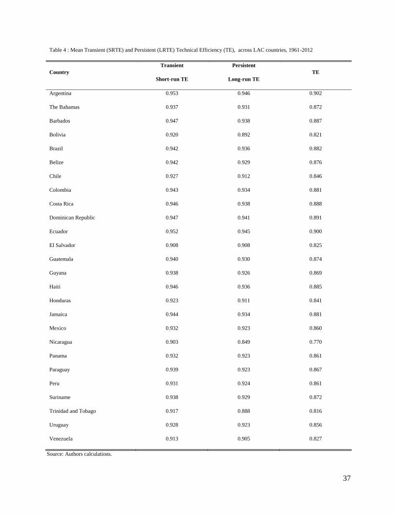
37

Table 4 : Mean Transient (SRTE) and Persistent (LRTE) Technical Efficiency (TE), across LAC countries, 1961-2012

Country

Transient

Short-run TE

Persistent

Long-run TE

TE

Argentina 0.953 0.946 0.902

The Bahamas 0.937 0.931 0.872

Barbados 0.947 0.938 0.887

Bolivia 0.920 0.892 0.821

Brazil 0.942 0.936 0.882

Belize 0.942 0.929 0.876

Chile 0.927 0.912 0.846

Colombia 0.943 0.934 0.881

Costa Rica 0.946 0.938 0.888

Dominican Republic 0.947 0.941 0.891

Ecuador 0.952 0.945 0.900

El Salvador 0.908 0.908 0.825

Guatemala 0.940 0.930 0.874

Guyana 0.938 0.926 0.869

Haiti 0.946 0.936 0.885

Honduras 0.923 0.911 0.841

Jamaica 0.944 0.934 0.881

Mexico 0.932 0.923 0.860

Nicaragua 0.903 0.849 0.770

Panama 0.932 0.923 0.861

Paraguay 0.939 0.923 0.867

Peru 0.931 0.924 0.861

Suriname 0.938 0.929 0.872

Trinidad and Tobago 0.917 0.888 0.816

Uruguay 0.928 0.923 0.856

Venezuela 0.913 0.905 0.827

Source: Authors calculations.

38

Table 5: Growth Rates of CATFP Components in LAC, 1961-2012

Country TE SE CATFP

Argentina -0.032 -0.002 1.052

Bahamas 0.175 -0.005 1.256

Barbados -0.028 0.001 1.057

Bolivia -0.111 -0.005 0.963

Brazil 0.071 -0.004 1.154

Belize -0.021 -0.007 1.060

Chile 0.245 -0.004 1.335

Colombia 0.032 -0.003 1.123

Costa Rica 0.172 -0.006 1.255

Dominican Republic 0.011 -0.003 1.099

Ecuador -0.041 -0.004 1.044

El Salvador -0.012 -0.002 1.071

Guatemala 0.120 -0.005 1.202

Guyana -0.015 -0.002 1.067

Haiti -0.145 -0.001 0.946

Honduras 0.008 -0.004 1.089

Jamaica 0.005 -0.001 1.092

Mexico 0.222 -0.004 1.304

Nicaragua -0.016 -0.004 1.065

Panama -0.228 -0.003 0.857

Paraguay -0.031 -0.005 1.056

Peru 0.038 -0.004 1.124

Suriname -0.087 -0.004 0.992

Trinidad and Tobago -0.488 0.000 0.586

Uruguay 0.053 -0.003 1.136

Venezuela 0.438 -0.004 1.522

LAC 0.014 -0.003 1.097

39

Table 6: Panel Unit Root Tests across sub-regions

South America Test p-value root

Levin-Lin-Chu (LLC) 2.99 0.99 I(1)

Im-Pesaran-Shin (IPS) -1.21 0.11 I(1)

Breitung 7.73 1 I(1)

Central America Test p-value root

Levin-Lin-Chu (LLC) 1.37 0.91 I(1)

Im-Pesaran-Shin (IPS) -1.46 0.07 I(1)

Breitung 6.32 1 I(1)

Caribbean Test p-value Root

Levin-Lin-Chu (LLC) 3.84 0.99 I(1)

Im-Pesaran-Shin (IPS) 2.67 0.99 I(1)

Breitung 7.17 1 I(1)

40

Table 7: Panel Cointegration test across LAC Sub-regions

Statistic

tests Value

Z-

value

P-

value

R. P

value Value

Z-

value

P-

value

R. P-

value Value

Z-

value

P-

value

R. P-

value

South America

Central America

Caribbean

Gt -3.1 -3.2 0.00 0.00 -2.5 -2.4 0.01 0.15 -2.7 -2.2 0.00 0.01

Ga -25.5 -6.8 0.00 0.01 -12.3 -2.7 0.01 0.18 -11.0 -1.5 0.00 0.06

Pt -9.2 -2.5 0.00 0.00 -6.7 -2.5 0.01 0.12 -5.3 -2.0 0.00 0.02

Pa -28.3 -10.8 0.00 0.01 -11.6 -4.5 0.00 0.15 -11.3 -3.4 0.00 0.00

Notes: These statistic tests are derived in Westerlund (2007)

R. : Robust

41

Table 8: Estimates for Error Correction Model (ECM)

Models Model PMG

Model MG

N=874 Coeff. S.E.

Coeff. S.E.

0.57a 0.057

0.8a 0.121

-0.91a 0.023

-0.97a 0.035

-0.24a 0.068

-0.40a 0.066

Log-likelihood 1373.9

Notes: a, b, c are 1%, 5%, and 10% level of significance respectively

S.E.: Standard error. Variables are measured in natural log.

42

Table 9: Economic Cost and productivity loss in LAC due to Climatic Variability by 2040

CATFP Growth

(%)

Present Value Loss (billion US $)

Discount Rate Discount Rate Discount Rate

0.5% 2% 4%

(A2)

(B2) (A2) (B2) (A2) (B2) (A2) (B2)

LAC w.r.t. Baseline -10.73 -2.35 89.1 33.2 58.9 21.9 34.2 12.7

Source: Authors calculations.

43

Figure 1: Effects of Maximum Temperature, Precipitation Anomaly and Rainy days on Output in LAC,

1961-2012

A. Maximum Temperature B. Precipitation

C. Rainy days

Source: Authors calculations based on FAO and CRU data.

-.4

-.2

0

.2

.4

Cha

ng

e in

Outp

ut (in

%)

27.5 28 28.5 29

Temperature (Degree Celcius)

-1.5

-1

-.5

0

Cha

ng

e in

Outp

ut (%

)

1960 1970 1980 1990 2000 2010

-.2

-.1

0

.1

.2

Cha

ng

e in

Outp

ut (in

%)

155 160 165 170 175

Rainy Days

44

Figure 2: Mean Climate Effects Index (CEI) across LAC countries, 1961-2012

Source: Authors calculations.

Figure 3: Relative change in output in LAC countries due to climatic variability

(1961-2000 vs 2001-2012) (%)

Source: Authors calculations.

.353

.354

.355

.356

.357

.358

Clim

ate

Effe

cts

Ind

ex (

CE

I)

1960 1970 1980 1990 2000 2010

-.05-1.15

-2.7-5.26

.88-.63

-1.93-3.64

1.22-2.51

-1.51-3.43

-5.31-1.92-1.97

-.13-3.32

-2.23.89

1.964.21

-.13-5.91

-7.32-12.53

2.61

-15 -10 -5 0 5Average Change in Output (in %)

Venezuela Uruguay

Trinidad and TobagoSuriname

PeruParaguayPanama

NicaraguaMexico

JamaicaHonduras

HaitiGuyana

GuatemalaEl Salvador

EcuadorDominican Republic

Costa RicaColombia

ChileBrazil

Bolivia Belize

BarbadosBahamasArgentina

45

Figure 4: Kernel Distribution of Persistent (LRTE) and Transient (SRTE) Technical Efficiency

across LAC countries

Source: Authors calculations.

Figure 5: Cumulative CATFP, TE, TC and SE in LAC, 1961-2012 (1961=1)

Source: Authors calculations.

Ker nel D ensity E stim ates

6 .0 7

1 2 .1 4

1 8 .2 0

2 4 .2 7

3 0 .3 4

.0 0

.7 0 .8 0 .9 0 1 .0 0.6 0

SRTE LRTE

De ns ity

1

1.1

1.2

1.3

1.4

1.5

Cum

ula

tive In

de

x (1

96

1=

1)

1960 1970 1980 1990 2000 2010

TE SE TP CATFP

46

Figure 6: Technical Efficiency “Catch-up” Index for LAC and Sub-regions, 1961-2012 (1961 = 1)

Source: Authors calculations.

.97

.98

.99

1

1.01

TE

(1

96

1=

1)

1960 1970 1980 1990 2000 2010

LAC

.98

.99

1

1.01

1.02

TE

(1

96

1=

1)

1960 1970 1980 1990 2000 2010

South America

.94

.96

.98

1

1.02

TE

(1

96

1=

1)

1960 1970 1980 1990 2000 2010

Caribbean

.94

.96

.98

1

1.02

TE

(1

96

1=

1)

1960 1970 1980 1990 2000 2010

Central America

.94

.96

.98

1

1.02

TE

(1

96

1=

1)

1960 1970 1980 1990 2000 2010

South America, Andean Region

.7

.8

.9

1

TE

(1

96

1=

1)

1960 1970 1980 1990 2000 2010

Trinidad & Tobago

.94

.96

.98

1

1.02

TE

(1

96

1=

1)

1960 1970 1980 1990 2000 2010

South America, South Cone Region

.8

.9

1

1.1

1.2

TE

(1

96

1=

1)

1960 1970 1980 1990 2000 2010

Chile

47

Figure 7: Structural break and Unit Root test for LAC and Sub-Regions, 1961-2012

Source: Authors calculations.

-.0

2-.

01

0

.01

.02

D.D

.TE

1960 1970 1980 1990 2000 2010

Latin America and the Caribbean

-8-7

.5-7

-6.5

Bre

akp

oin

t t-

sta

tistic

1960 1970 1980 1990 2000 2010

Breakpoint t-statistic: min at 1988

in series: D.TE

Clemente-Montañés-Reyes single AO test for unit root

-.0

4-.

02

0

.02

.04

D.D

.TE

1960 1970 1980 1990 2000 2010

South America

-6.6

-6.4

-6.2

-6-5

.8-5

.6

Bre

akp

oin

t t-

sta

tistic

1960 1970 1980 1990 2000 2010

Breakpoint t-statistic: min at 1976

in series: D.TE

Clemente-Montañés-Reyes single AO test for unit root

-.04

-.02

0

.02

.04

D.D

.TE

1960 1970 1980 1990 2000 2010

Carribean

-10

-9.5

-9

-8.5

Bre

akpo

int t-

sta

tistic

1960 1970 1980 1990 2000 2010

Breakpoint t-statistic: min at 2005

in series: D.TE

Clemente-Montañés-Reyes single AO test for unit root

-.04

-.02

0

.02

.04

D.D

.TE

1960 1970 1980 1990 2000 2010

Central America

-6

-5.8

-5.6

-5.4

-5.2

-5

Bre

akpo

int t-

sta

tistic

1960 1970 1980 1990 2000 2010

Breakpoint t-statistic: min at 2000

in series: D.TE

Clemente-Montañés-Reyes single AO test for unit root

48

Figure 8: Historical and Projected Cumulative CATFP across LAC countries, 1961-2040 (1961=1)

Source: Authors calculations.

1

1.5

2

2.5In

de

xes

1960 1980 2000 2020 2040

CATFP_Baseline CATFP_B2 CATFP_ A2

49

APPENDIXES

Table A: Projected Mean of Climate Variables w.r.t. to the IPCC baseline (1960-1990)

Scenario A2 Scenario B2 Scenario A2 Scenario B2

Bahamas 1.53 1.75 -9.8 -12.41

Barbados 1.86 1.93 -4.15 -24.07

Belize 2.38 2.39 -13.56 -5.5

DR 1.81 2.13 10.18 5.74

Guyana 2.73 3.16 11.59 -7.3

Haiti 2.01 2.05 23.34 24.38

Jamaica 1.66 1.75 -16.99 -20.85

Trinidad 2.27 2.53 12.24 -16.49

Suriname 1.8 1.89 -4.03 -11.51

Average 1.8 1.89 -4.03 -11.51

Costa Rica 1.6 1.23 -12.47 -3.08

El Salvador 2.03 1.4 -15.23 -2.44

Guatemala 2 1.43 -12.73 -0.1

Honduras 1.83 1.4 -15.7 -7.18

Panama 1.4 1.23 -7.97 -2.36

Nicaragua 1.9 1.37 -17.93 -7.31

Mexico 1.73 1.33 -13.87 -4.33

Average 1.73 1.33 -13.87 -4.33

South America 4 2.5 -40 -20

Maximum Temperature Precipitation

50

REFERENCES

Andressen, R., L. F. Terceros and M. Monasterio, (2000). “The role of climate in the

desertification process of the southern Bolivian high plains.” in Proceedings of the

Meeting of Experts from Regional Associations III and IV on Extreme Events” Caracas,

Venezuela,World Meteorological Organization, Geneva, Switzerland, pp. 55–75.

Ball, V. E., C. Hallahan and R. Nehring. (2004). “Convergence of productivity: an analysis of

the catch-up hypothesis within a panel of states.” American Journal of Agricultural

Economics, 86(5): 1315-1321.

Baltagi, B. (2008). “Econometric analysis of panel data.” John Wiley & Sons, Vol. 1.

Banerjee, A., J. Dolado and R. Mestre. (1998). “Error‐ correction mechanism tests for

cointegration in a single‐ equation framework.” Journal of time series analysis, 19(3):

267-283.

Barro, R. J. (1991). “Economic growth in a cross section of countries”. Quarterly Journal of

Economics, 106(2): 407-443.

Barro, R. J. (1997). “The Determinants of economic growth: a cross-country empirical study.”

MIT Press, Cambridge.

Barnwal, P., and K. Kotani. (2013). “Climatic impacts across agricultural crop yield

distributions: an application of quantile regression on rice crops in Andhra Pradesh,

India.” Ecological Economics, 87: 95-109.

Baumol, W. J. (1986). “Productivity growth, convergence, and welfare: what the long-run data

show.” The American Economic Review, 76(5): 1072-1085.

Bernard A. B., and C. I. Jones. (1996). “Comparing apples to oranges: productivity convergence

and measurement across industries and countries.” The American Economic Review,

86(5): 1216-1238.

Bhat, C. R. (2001). “Quasi-random maximum simulated likelihood estimation of the mixed

multinomial logit model.” Methodological, 35(7): 677-693.

Boshrabadi, H. M., R. Villano and E. Fleming. (2008). “Technical efficiency and

environmental‐ technological gaps in wheat production in Kerman province of Iran.”

Agricultural Economics, 38(1): 67-76.

Breitung, J. (2000). “The local power of some unit root tests for panel data.” In: B. H. Baltagi

(ed.) Nonstationary Panels, Panel Cointegration, and Dynamic Panels. Amsterdam:

Elsevier, pp. 161–177.

Bruckner, M., and A. Ciccone. (2011). “Rain and the democratic window of opportunity.”

Econometrica, 79 (3): 923–47.

51

Burke, P. J., and A. Leigh, (2010). “Do output contractions trigger democratic change?”

American Economic Journal Macroeconomics, 2(4): 124-157.

Butler, J. S., and R. Moffitt. (1982). “A computationally efficient quadrature procedure for the

one-factor multinomial probit model.” Econometrica, 50(3): 761-764.

Catao, L. A., and M. E. Terrones. (2005). “Fiscal deficits and inflation.” Journal of Monetary

Economics, 52(3): 529-554.

Cheesman, J., J. Bennett and T. V. H. Son. (2008). “Estimating household water demand using

revealed and contingent behaviors: evidence from Vietnam.” Water Resources Research,

44 (11):1-11.

Chomitz, K. M., P. Buys, G. De Luca, T. S. Thomas and S. WertzKanounnikoffand. (2007). “At

Loggerheads? agricultural expansion, poverty reduction, and environment in the tropical

forests.” The World Bank report, Washington,DC.

Chou, C., C. A. Chen, P. H. Tan and K. T. Chen, (2012). “Mechanisms for global warming

impacts on precipitation frequency and intensity.” Journal of Climate, 25(9): 3291-3306.

Clemente, J., A. Montanes, and M. Reyes. (1998). “Testing for a unit root in variables with a

double change in the mean.” Economics Letters, 59(2): 175-182.

Colombi, R., S. C. Kumbhakar, G. Martini and G. Vittadini. (2011). “A stochastic frontier model

with short-run and long-run inefficiency.” Unpublished manuscript, University of

Bergamo.

Colombi, R., S. C. Kumbhakar, G. Martini and G. Vittadini. (2014). “Closed-skew normality in

stochastic frontiers with individual effects and long/short-run efficiency.” Journal of

Productivity Analysis, 42(2):123–136.

Corbo, V. and K. Schmidt-Hebbel. (2013). “The international crisis and Latin America.”

Monetaria 35(1): 37-62.

Cornwell, C. M., and J. U. Wächter. (1999). “Productivity convergence and economic growth: a

frontier production function approach.” ZEI working paper, No. B 06-1999.

Cotrina, J. S. (2000). “Evaluation of the ENSO phenomena impact on agriculture in Peru,” in

Proceedings of the Meeting of Experts from Regional Associations III and IV on Extreme

Events, Caracas, Venezuela, World Meteorological Organization, Geneva, Switzerland,

pp. 135–151.

Dell, M., B. F. Jones and B. A. Olken. (2012). “Temperature shocks and economic growth:

Evidence from the last half century.” American Economic Journal Macroeconomics,

4(3): 66-95.

Dell, M., B. F. Jones and B. A. Olken, (2014). “What do we learn from the weather? the new

climate-economy literature.” Journal of Economic Literature, 52(3): 740-98.

52

De Long, J. B. (1988). “Productivity growth, convergence, and welfare: comment.” The

American Economic Review, 78(5): 1138-1154.

ECLAC (2014). “Economics of climate change in Latin America and the Caribbean. Summary

2010.” Santiago, Chile.

ECLAC (2010). “The economics of climate change in Latin America and the Caribbean:

Paradoxes and challenges.”Santiago, Chile.

Food and Agriculture Organization of the United Nations (FAO) (2010). “Global Forest

Resources Assessment 2010: Main Report.” FAO Forestry Paper No. 163. Food and

Agriculture Organization of the United Nations. Rome.

FAOSTAT (2014). “Statistical database.” Retrieved September 2014, from

http://faostat.fao.org/site/339/default.aspx.

Farsi, M., M. Filippini and W. Greene (2005). “Efficiency measurement in network industries:

application to the Swiss railway companies.” Journal of Regulatory Economics, 28 (1):

69–90

Fedderke, J. (2004). “Investment in fixed capital stock: testing for the impact of sectoral and

systemic uncertainty.” Oxford Bulletin of Economics and Statistics, 66(2): 165-187.

Federico, G. (2005).“Feeding the world: an economic history of agriculture, 1800-2000.”

Princeton University Press.

Filippini, M., and W. H. Greene. (2014). “Persistent and transient productive inefficiency: a

aaximum simulated likelihood approach.” CER-ETH–Center of Economic Research at

ETH Zurich Working Paper, (14/197).

Fulginiti, L. E., R. K. Perrin, and B. Yu, (2004). “Institutions and agricultural productivity in

Sub-Saharan Africa.” Agricultural Economics, 31(2-3), 169-180.

Geist, H. and E. Lambin. (2002). “Proximate causes and underlying driving forces of tropical

deforestation.” Bioscience, 52(2): 143-150.

Glynn, J., N. Perera and R. Verma. (2007). “Unit root tests and structural breaks: a survey with

applications.” Faculty of Commerce-Papers, 455.

Greene, W. H. (2005a). “Reconsidering heterogeneity in panel data estimators of the stochastic

frontier model.” Journal of Econometrics, 126(2):269-303.

Greene, W. H. (2005b). “Fixed and random effects in stochastic frontier models.” Journal of

Productivity Analysis, 23(1): 7-32.

Greene, W. H. (2008). “Econometric analysis.” Englewood Cliffs, NJ: Prentice Hall.

Greene, W. H. (2001). “Fixed and random effects in nonlinear models.” Department of

Economics, Stern School of Business, New York University, Working Paper Number 01–

01.

53

Greene, W. H. (2012). “LIMDEP version 10.0: user’s manual and reference guide.” New York:

Econometric Software.

Hamilton, J. D. (1994). “Time series analysis.” Princeton: Princeton university press, Vol. 2.

Harris, I., P. D. Jones, T. J. Osborn and D. H. Lister. (2014). “Updated high-resolution grids of

monthly climatic observations–the CRU TS3. 10 Dataset.” International Journal of

Climatology, 34(3): 623-642.

Hazell, P. and A. Roell. (1983). “Rural growth linkages: household expenditure patterns in

Malaysia and Nigeria.” IFPRI Research Report, No. 41, IFPRI, Washington, DC.

Hughes, N., K. Lawson, A. Davidson, T. Jackson and Y. Sheng, (2011). “Productivity pathways:

climate adjusted production frontiers for the Australian broadacre cropping industry.”

ABARES report, Australia.

Hsiang, S. M., and A. S. Jina. (2014). “The causal effect of environmental catastrophe on long-

run economic growth: Evidence From 6,700 Cyclones.” NBER Working Paper No.

20352.

Im, K. S., M. H. Pesaran and Y. Shin. (2003). “Testing for unit roots in heterogeneous panels.”

Journal of Econometrics, 115(1):53-74.

IPCC (2014a). “Climate change 2014: impacts, adaptation, and vulnerability.” Contribution of

Working Group II to the Fifth assessment report of the Intergovernmental Panel on

Climate Change, Barros, V. R., and others (eds.), Cambridge, Cambridge University

Press

IPCC (2014b). “Summary for policymakers.” Global and sectoral aspects. Climate change 2014:

impacts, adaptation, and vulnerability. Contribution of Working Group II to the fifth

assessment report of the Intergovernmental Panel on Climate Change, Field, C. B. and

others (eds.), Cambridge, Cambridge University Press.

James, R. and R. Washington (2013). “Changes in African temperature and precipitation

associated with degrees of global warming.” Climatic Change, 117(4): 859-872.

Jondrow, J., C. A. Knox Lovell, I. S. Materov and P. Schmidt. (1982). “On the estimation of

technical inefficiency in the stochastic frontier production function model.” Journal of

Econometrics, 19(2): 233-238.

Kim, D. H., S. C. Lin and Y. B. Suen, (2010). “Dynamic effects of trade openness on financial

development.” Economic Modelling, 27(1):254-261.

Kremers J. J., N. R. Ericsson and J. J. Dolado (1992). “The power of co-integration tests.”

Oxford bulletin of economics and statistics, 54(3): 325-348.

Krueger, A.O., M. Schiff, and A. Valdes. (1991). “The political economy of agricultural pricing

policy.” Vol 1: Latin America. Vol 2: Asia. Johns Hopkins University Press.

54

Kumar, S., and R. R. Russell. (2002). “Technological change, technological catch-up, and capital

deepening: relative contributions to growth and convergence.” The American Economic

Review, 92(3):527-548.

Kumar, S., B. M. K. Raju, C. A. R. Rao, K. Kareemulla and B. Venkateswarlu. (2011).

“Sensitivity of yields of major rainfed crops to climate in India.” Indian Journal of

Agricultural Economics, 66(3): 340-352.

Kumbhakar, S. C. and E. G. Tsionas. (2005). “Measuring technical and allocative inefficiency in

the translog cost system: a Bayesian approach.” Journal of Econometrics, 126(2): 355-

384.

Kumbhakar, S. C., G. Lien and J. B. Hardaker. (2014). “Technical efficiency in competing panel

data models: a study of Norwegian grain farming.” Journal of Productivity Analysis,

41(2): 321-337.

Lachaud, M. A. (2014). “Three Essays on Resource Use, Sustainability and Agricultural

Productivity.” PhD thesis, Digital Commons, University of Connecticut, Storrs.

Lachaud, M. A., B. E. Bravo-Ureta and C. E. Ludena. (2015). “Agricultural productivity gaps in

Latin America and the Caribbean in the presence of unobserved heterogeneity and

climatic effects: a comparison of alternative model specifications.” Working paper,

University of Connecticut, Storrs.

Levin, A., C. Lin and C. Chu. (2002). “Unit root tests in panel data: Asymptotic and finite-

sample properties.” Journal of Econometrics, 108(1):1-24.

Liu, Y., C. R. Shumway, R. Rosenman and V. E. Ball. (2011). “Productivity growth and

convergence in U.S. agriculture: new cointegration panel data results.” Applied

Economics, 43(1):91-102.

Loayza, N. and P. Fajnzylber. (2005). “Economic growth in Latin America and the Caribbean:

stylized facts, explanations, and forecasts.” World Bank Publications, Washington, DC.

Lobell, D., J. Costa-Roberts, W. Schlenker. (2011). “Climate trends and global crop production

since 1980.” Science, 333 (6042):616-620.

Ludena, C. E., T. W. Hertel, P. V. Preckel and A. Nin. (2007). “Productivity growth and

convergence in crop, ruminant and non-ruminant production: measurement and

forecasts.” Agricultural Economics, 37(1): 1-17.

Ludena, C. E. (2010). “Agricultural productivity growth, efficiency change and technical

progress in Latin America and the Caribbean.” IDB Working Paper Series, No. 186.

Maccini, S. and D. Yang. (2009). “Under the weather: health, schooling, and economic

consequences of early-life rainfall.” The American Economic Review, 99(3): 1006-1026.

Mankiw, N. G., D. Romer and D. N. Weil. (1992). “A contribution to the empirics of economic

growth.” Quarterly Journal of Economics, 107(2): 407-437.

55

Müller, C., A. Bondeau, A. Popp, K. Waha and M. Fader. (2010). “Climate change impacts on

agricultural yields.”In Development and Climate Change. World Development, Report.

Mendelsohn, R. and A. Dinar. (2003). “Climate, water, and agriculture.” Land Economics, 79(3):

328–341.

Mukherjee, D., B. E. Bravo-Ureta and A. de Vries. (2013). “Dairy productivity and climatic

conditions: econometric evidence from South-eastern United States.” Australian Journal

of Agricultural and Resource Economics, 57(1): 123-140.

Mundlak, Y. (1978). “On the pooling of time series and cross section data.” Econometrica,

46(1): 69-85.

Nelson, G. C., M. W. Rosegrant, J. Koo, R. Robertson, T. Sulser, T. Zhu, C. Ringler, S. Msangi,

A. Palazzo, M. Batka, M. Magalhaes, R. Valmonte-Santos, M. Ewing and D. Lee. (2009).

“Climate change: Impact on agriculture and costs of adaptation.” International Food

Policy Research Institute (IFPRI), Washington, DC.

Nin‐ Pratt, A. and B. Yu. (2010). “Getting implicit shadow prices right for the estimation of the

Malmquist index: the case of agricultural total factor productivity in developing

countries.” Agricultural Economics, 41(3-4), 349-360.

Njoupouognigni, M. (2010). “Foreign aid, foreign direct investment and economic growth in

Sub-Saharan Africa: evidence from pooled mean group estimator (PMG).” International

Journal of Economics and Finance, 2(3): 39-45.

O'Donnell, C. J. (2010) “Measuring and decomposing agricultural productivity and profitability

change.” Australian Journal of Agricultural and Resource Economics 54(4):527-560.

O’Donnell C. J. (2012). “An aggregate quantity framework for measuring and decomposing

productivity change.” Journal of Productivity Analysis, 38(3):255-272.

O’Donnell C. J., and K. Nguyen. (2012). “An econometric approach to estimating support prices

and measures of productivity change in public hospitals.” Journal of Productivity

Analysis, 40(3):323-335.

Pesaran, M. H., Y. Shin and R. P. Smith (1997). “Estimating long-run relationships in dynamic

heterogeneous panels.” DAE Working Papers Amalgamated, Series 9721.

Pesaran, M. H., Y. Shin and R. P. Smith (1999). “Pooled mean group estimation of dynamic

heterogeneous panels.” Journal of the American Statistical Association, 94(446): 621-

634.

Pesaran, M. H. and R. Smith (1995). “Estimating long-run relationships from dynamic

heterogeneous panels.” Journal of Econometrics, 68(1): 79-113.

Peterson, T. C., T. R. Karl, P. F. Jamason, R. Knight and D. R. Easterling. (1998). “First

difference method: maximizing station density for the calculation of long-term global

56

temperature change.” Journal of Geophysical Research: Atmospheres, 03(D20): 25967-

25974.

Phillips, P. C. and H. R. Moon. (2000). “Nonstationary panel data analysis: an overview of some

recent developments.” Econometric Reviews, 19(3): 263-286.

Rabe-Hesketh, S. and A. Skrondal. (2005). “Multilevel and Longitudinal Modeling Using

Stata.” College Station, TX: Stata Press.

Rahman, S. (2011). “Resource use efficiency under self-selectivity: the case of Bangladeshi rice

producers.” Australian Journal of Agricultural and Resource Economics, 55(2): 273-290.

Rao D. P. and T. J. Coelli. (2004). “Catch-up and convergence in global agricultural

productivity.” Indian Economic Review, 39(1):123-148.

Rassenfosse G. D. and B. Potterie (2012). “On the price elasticity of demand for patents.” Oxford

Bulletin of Economics and Statistics, 74(1): 58-77.

Solow, R. M. (1956). “A contribution to the theory of economic growth.” Quarterly Journal of

Economics, 70(1): 65-94.

Stern, N. (2013). “The structure of economic modeling of the potential impacts of climate

change: grafting gross underestimation of risk onto already narrow science models.”

Journal of Economic Literature, 51(3): 838-859.

Suhariyanto, K., and C. Thirtle. (2001). “Asian agricultural productivity and convergence.”

Journal of Agricultural Economics, 52(3): 96-110.

Train, K., (2002). “Discrete choice: methods with simulation.” Cambridge University Press,

Cambridge.

Tsionas, E. G. and S. C. Kumbhakar. (2014). “Firm heterogeneity, persistent and transient

technical inefficiency: a generalized True random Effects model.” Journal of Applied

Econometrics, 29(1): 110-132.

University of East Anglia Climatic Research Unit (CRU) (2013). [Phil Jones, Ian Harris]. “CRU

TS3.21: Climatic Research Unit (CRU) Time-Series (TS) Version 3.21 of high resolution

gridded data of month-by-month variation in climate (Jan. 1901 - Dec. 2012), [Internet].”

NCAS British Atmospheric Data Centre, 2013, Date of citation. Available from

http://badc.nerc.ac.uk/browse/badc/cru/data/cru_cy/cru_cy_3.21/data

Vergara, W., A. R. Rios, L. M. Galindo, P. Gutman, P. Isbell, P. H. Suding and R. Pachauri,

(2013). “The climate and development challenge for Latin America and the Caribbean:

options for climate-resilient, low-carbon development.” Inter-American Development

Bank, Washington, DC.

Wani, S. P., J. Rockström and T. Y. Oweis, (eds.). (2009). “Rainfed agriculture: unlocking the

potential.” CABI North American Office, Cambridge MA.

57

Westerlund, J. (2007). “Testing for error correction in panel data.” Oxford Bulletin of Economics

and Statistics, 69(6): 709-748.

Wooldridge, J. M. (2002). “Econometric analysis of cross section and panel data: MIT press.

World Bank (2003). “Rural poverty report.” The World Bank, Washington, DC.

World Bank (2008). “World Development Report 2008: agriculture for development.” The

World Bank, Washington, DC.

World Bank (2012). “Climate change: is Latin America prepared for temperatures to rise 4

degrees?” Retrieved September 1, 2013, from

http://www.worldbank.org/en/news/feature/2012/11/19/climate-change-4-degrees-latin-

america-preparation