agricultural and environmental efficiency implications ... s... · transboundary externalities...
TRANSCRIPT

AGRICULTURAL AND ENVIRONMENTAL EFFICIENCY - IMPLICATIONS
FOR THE REGIONAL INTEGRATION OF THE CARIBBEAN ISLANDS Johannes Sauer Institute of Food and Resource Economics Royal Veterinary and Agricultural University Copenhagen, Denmark Email: [email protected]
Sonja S. Teelucksingh Economics Department The University of the West Indies St. Augustine, Trinidad Email: [email protected]
Abstract Much of the utilised land in Caribbean islands is coastal zone, with highly interlinked terrestrial and marine ecosystems. Marine resources available to island states can, if properly utilised, significantly contribute to the sustainable development of the Caribbean region. Developmental strategies that compromise the integrity of this resource can have devastating effects. The Caribbean islands were historically monocrop agricultural economies, and agriculture continues to play an important socio-economic role in the livelihoods of Caribbean peoples. In islands with a heavy reliance on coastal zone areas, the agricultural sectors can pose significant transboundary externalities to Caribbean Sea ecosystems and, from the human harvesting perspective, the fisheries sectors in particular in terms of agricultural run off into the marine environment. Given geographical proximity, shared marine resources, land-ocean interactions and transboundary externalities resulting from non-point sources of pollution, the environmental challenges facing the islands of the Caribbean Sea can only be effectively addressed by cross-country efforts under the umbrella of increased regional cooperation. This paper seeks to address these issues in the context of regional integration. In a first step we investigate the relative efficiency of agricultural production on selected Caribbean islands by means of stochastic efficiency analysis. Based on this analysis we then focus possible lines of production specialisation in terms of relative comparative advantages. This single sector approach is then modified by incorporating environmental linkages between the agricultural and fisheries sectors of the selected islands. Finally, post-integration scenarios are built based not only on inter-island relative productive efficiencies of the agricultural sectors but also on inter-sectoral relative environmental efficiencies from a multi-sectoral point of view.

2
Paper Outline Introduction research question data set method results implications

3
1 - Introduction The issue of natural resource management is a crucial one, particularly so in small island economies where a heavy reliance on natural resource exploitation is coupled with a vulnerability to external economic and environmental factors. Small island economies generally share a number of characteristics (Bass 1993). Small populations and high population densities lead to high demands on natural resources. Island ecosystems are intimately linked. A high ratio of coastal to land area leaves islands vulnerable to internal and external ecological influences. Islands are characterised by environmental fragility, with a delicate balance existing between highly coupled terrestrial and marine ecosystems (Mc Elroy et al, 1990). The “Caribbean Economy” of today is now identifiable by characteristics that have their origins in the “plantation economy” – a monocrop economy with a large export sector based on natural resource exploitation. There exists a high propensity of import consumption. In the extreme cases, it produces what it does not consume and consumes what it does not produce. The economy is a price taker, reactive rather than proactive, and hence is highly vulnerable to changes in the global economic climate. The Caribbean Economy remains dependent on the developed world for absorption of its exports and as the source of its imports, its capital and entrepreneurship and even its skilled labour. These structural characteristics imply a certain set of vulnerabilities of such an economy to both the external economic climate and the surrounding and all encompassing natural environment. Both in an historic and a contemporary sense, island economies have supported themselves by wholesale biomass removal, accompanied by substantial environmental degradation (McElroy et. al 1990, Bass 1993). The last two decades have seen a growing awareness of environmental issues the world over, and the Caribbean region has been no exception. As early as 1973, there was documented concern about marine pollution issues in the region (UNEP 1994). Coastal degradation and marine pollution have since become serious and important issues (Siung-Chang, 1997). The surrounding marine environment and its quality impacts upon all aspects of life in the Caribbean (Roberts et. al, 1995). Indeed, for many small islands the marine environment can be the most important economic resource (Bass, 1993). Developmental strategies that compromise the integrity of this resource can have devastating effects, both in an immediate sense as well as in the longer term. The interlinked island ecosystems will respond to changes in one of the constituent parts. Furthermore, as the economy begins to respond to the environmental changes, shifts in the economic structure itself will impact the way in which the environmental resources are exploited. In the end, if development occurs at overbearing costs to the marine environmental quality, it is the poorest members of the society who will suffer the most (Roberts et. al, 1995).

4
The Caribbean Region The “Caribbean Region” can be geographically defined in a number of ways. The broadest definition is that utilised by the 1983 Convention for the Protection and Development of the Marine Environment of the Wider Caribbean Region (WCR), more commonly known as the Cartagena Convention (see Figure 1). Here the “Convention Area” was defined as follows – “....the marine environment of the Gulf of Mexico, the Caribbean Sea and areas of the Atlantic Ocean adjacent thereto, south of 30’ north latitude and within 200 nautical miles of the Atlantic coast of the States referred to in article 25 of the Convention” (UNEP 1994) This definition encompasses twelve continental States, thirteen island States, the Commonwealth of Puerto Rico, three overseas departments of France, a Territory shared by the Netherlands and France (St. Martin) and eleven dependent territories (UNEP 1994). The Wider Caribbean Region as defined by the Cartagena Convention represents over forty discrete political entities with a rich and diverse heritage. It is a melting pot of cultures, languages, societal structure and economic capabilities (Fabres 1996, Montero 2002). The Caribbean Sea of this region is an immense expanse that is downstream from major continental river systems that generate over 20% of fresh water and 12% of sediment outflows into the Atlantic Ocean. The region also receives major inflows of deep water from the Atlantic. The Caribbean sea contains an estimated 9% of global coral reef area and a human population of over 230 million people, with over 50 million living in coastal areas (Fabres 1996). The Role of the Natural Environment In all economies, the natural environment has at least three clear roles to play. Firstly, it is the source of the environmental inputs into the production of the domestic sectors of the economy. Secondly, it acts as the receptor or “waste-sink” of these productive activities, in as much as its limited assimilative capacity allows. Finally, the environment has value in its own right to the welfare of the economy (the amenity value). As the common source of key environmental inputs into production, the natural environment accounts for an interdependence between domestic productive sectors and also the medium through which externalities can arise. Although the role of non-marketed environmental inputs can theoretically be captured by market-based instruments such as royalties and licenses for access to environmentally fragile sites, there exists no market to account for the environmental impacts that one sector can potentially have on another and the negative externalities that arise from this. The question of externalities becomes crucial when dealing with an economy such as the one that has been defined - small, highly open, highly linked in the resource dependence of its two sectors and highly vulnerable to global economic shifts and changes. The physical and geographical landscape of any island economy leads to the existence of a close linkage and a delicate balance between terrestrial activities and the surrounding environment, in particular the marine ecosystems that surround it. This means that, though different environmental resources may play a specific role in production, the environmental linkage between them can lead to the existence of externalities. Though productive sectors may utilise different natural resources in production, the resources are themselves linked

5
through some ecological system which means that the production decisions and activities of one sector impacts upon the other and externalities arise in this way. Fisheries and Agriculture in the Caribbean For small island developing states in particular, the small-scale fisheries and agricultural sectors play a critical socio-economic role. While some islands are able to exploit indigenous mineral resources, tourism has replaced the sugar plantations as the monocrop of most small Caribbean islands. Fisheries and agriculture in the Caribbean islands continue to be, for the most part, small-scale and artisanal, an avenue of employment for much of the poorer classes of society. Despite small percentage contributions to aggregate GDP, there are substantial, indirect non-economic benefits derived. Fish provides the basic source of animal protein for many SIDS, and figures heavily in the food security equation in these countries (FAO 1999). The fisheries sector is important not only as the provider of this food resource but also because it is an avenue for self-employment and in the case of industrial fisheries, paid employment - this in a developing world context where employment opportunities are increasingly limited and labour decreasingly mobile across and between sectors due to sector industrialisation, and lack of skill and education as a barrier to entry. The harvesting and marketing of the resource both from small scale and industrial fleets, can also present opportunities to the inhabitants to participate in an economic activity to which in some cases they would not otherwise have access. The nature of the problem facing SIDS in terms of optimal utilisation of fishery resources at one point in time or its sustainable utilisation over the future time period are the same as that faced by larger states the world over. The difference, however, lies in the intensification of the problem due to a number of factors. Physically, the small size of the island states means that the opportunities for land-based development are limited, and so the sea and its resources play an increasingly critical role in the lives and economy of its inhabitants. Ecologically, the terrestrial and marine ecosystems of SIDS are essentially self-contained, leading to the quicker and more intense manifestation of problems than would be the case in larger, more developed continental states. Economically, the SIDS do not have access to the economic resources that would lead to choice and exercise of one of the range of solutions that (theoretically) the more developed states possess. It is commonly accepted that the marine resources available to island states can, if properly utilised, significantly contribute to the sustainable development of the region. Dolman (1990) further argues that it is the specific development of artisanal as opposed to industrial fisheries that is the key to sustainable social and economic development. He suggests that island states are not economically able to deal with the requirements and uncertainties associated with the development of industrial fisheries, that such development would lead to few employment opportunities and in many cases all that an industrial fishery focus would serve to do would be to magnify existing social and economic inequalities. He argues that with proper management and planning, an artisanal fishery focus would be cheaper, create more employment, contribute to national nutritional objectives and help to promote a more equitable income distribution. In short, while traditionally undervalued and neglected, it is the traditional small-scale artisanal fishery that is the most viable backbone of the increasingly socio-economically important fisheries sector.

6
For small island developing states in particular, the fisheries sector plays a critical socio-economic role. It is commonly accepted that the marine resources available to island states can, if properly utilised, significantly contribute to the sustainable development of the region. It has been further argued that it is the specific development of artisanal as opposed to industrial fisheries that is the key to sustainable social and economic development. Despite small percentage contributions to aggregate GDP, there are substantial, indirect non-economic benefits derived. Fish provides the basic source of animal protein for many SIDS, and figures heavily in the food security equation in these countries. The fisheries sector is important not only as the provider of this food resource but also because it is an avenue for self-employment - this in a developing world context where employment opportunities are increasingly limited and labour decreasingly mobile across and between sectors due to sector industrialisation, and lack of skill and education as a barrier to entry. The small-scale harvesting and marketing of the can also present opportunities to the inhabitants to participate in an economic activity to which in some cases they would not otherwise have access. The Perturbation of the Marine Environment The activities of a fishery itself can cause disruption in the ecological system. Unmanaged or mismanaged harvests can affect both the population biology of the ecosystem, as well as the physical habitat within which the species of the ecosystem exist. The immediate removal of large numbers of individuals of one species can affect the dynamics of all other species in the system. Furthermore, if the ability of a species to regenerate itself in the future time period is threatened by excessive harvests in the present, this can mean that not only are future harvests under threat but also the stability of the whole ecosystem. Depending on the nature of effort, excessive and even moderate levels of effort can also have a negative impact on the physical characteristics of the system. In the case of shrimp fisheries in particular, the trawling method of harvest is viewed as particularly physically detrimental to marine habitats as well as notoriously low in terms of the ratio of the target catch to non-target species or bycatch. These effects are what motivate traditional fishery regulation. Damaging environmental effects can also result from production or consumption activities that are independent of the fishery sector. In island economies, small land size and increasing population pressures mean that there is a magnified link between terrestrial activities and the marine environment. Land based activities can unknowingly cause both natural parameter shifts as well as the introduction of toxic substances into the marine ecological systems, which can have both a direct impact on a target species as well as an indirect impact on species to which they are trophically linked. If terrestrial or coastal zone activities can have a harmful impact on the surrounding or adjoining marine environment upon which the fishery harvests depend1, and if this impact is not reflected in market prices, we have a classical negative externality. This is what motivates the environmental regulation of terrestrial activities. Physical, chemical and biological changes in the marine environment within which species reside can operate in one of three ways. Any ecosystem and its component species and natural habitats are characterised by and accustomed to certain levels of physiochemical factors such as temperature, salinity, light intensities, acidity/alkalinity, dissolved oxygen concentration and oceanographic parameters such as winds and currents. The resilience of a
1 Of course, fishery harvests are only one of the benefits of the marine environment, and its degradation implies
many other negative impacts on society of which loss of harvest is but one.

7
marine ecosystem is measured by its ability to adjust to changes in these parameters. One effect of perturbations to the system is a change in these natural parameters. Marine ecosystems can also be perturbed by the introduction of toxic and alien substances into its ecological processes. The species and habitats that comprise the ecosystem are then forced to adapt to the substance, either by altering its chemical state to a less toxic nature by natural processes, or by assimilating and excreting the substance. Ecosystems are capable of performing these functions, in particular when the substance is one that can be naturally occurring in small, background levels in the marine environment, such as hydrocarbon inflow through natural seeps. The ability of an ecosystem to adapt to and assimilate potentially toxic chemicals is another feature of ecosystem resilience. Thirdly, marine organisms, though they may themselves be adaptable enough to withstand natural parameter shifts or the introduction of toxic substances into the ecosystem within which they exist, can be indirectly affected by the changes that these stresses can induce in other more vulnerable species of the ecosystem. This is through the trophic dynamics that exist within an ecosystem and the predator-prey relationships that result. Though morbidity and mortality of a species may not be directly induced by ecosystem perturbations, this could be the end result if the organisms or vegetation upon which the species are dependent as a food source are negatively affected by the changes. Furthermore, in terms of ecosystem health as a whole, negative consequences as a result of changing species composition can occur if there exists predator elimination and so the population explosion of the former prey. These three potential channels through which marine ecosystems can be affected by human-induced activities are not independent of each other but on the contrary inextricably linked. Toxic substances can themselves cause natural parameter shifts as the natural processes of the ecosystem attempt to assimilate the substance or reduce it to a less toxic nature. Alternatively, it can sometimes be the natural parameter levels that determine the assimilative capacity of an ecosystem and so impact the final toxicity levels of the substance. It can also be that certain species that are characterised by a greater sensitivity to physiochemical factors and possess less of an adaptability to changes in these factors through a smaller range of tolerance can be eliminated from an ecosystem by large parameter shifts, leading to trophic adjustment. Though it can be convenient to categorise ecosystem effects, it is essential to know that this is a simplification of the problem and that the reality is that an ecosystem is a complex and interlinking web. No general statement can be made on the consequences for fish populations and a whole and individual species in particular of ecosystem alterations as a result of toxic injections or natural parameter shifts. It must be recognised that the severity of such effects will depend on a host of variables that include climatological factors (the season in which the pollution occurs), oceanographic parameters (winds, currents), and the chemical nature of the pollutant and the timing and intensity of its release. The life history of the species in question is also of particular importance, where there is the potential for varying sensitivities to environmental alterations at different life stages. The tendency of some species to have different geographical preferences and occupy different positions in the water column or sediment at different life stages also means that there are varying degrees of exposure to a pollutant across the life history of a species. The key question becomes the extent to which both the ecological systems as well as the species themselves can withstand and absorb environmental changes with limited habitat and behavioural effects. The answer to this question is a complex one, dependent upon the

8
assimilative capacity of the system (itself dependent on the nature, type, levels and timing of the introduction of the toxic substance into its parameters) as well as the nature of the species that reside within the system, their physical and physiological characteristics, their sensitivity to and so the extent to which they respond to the natural parameters from one life stage to the next, and the capacity of these species to adapt to the changing parameters of the ecological system within which they reside. Land-Based Pollution in the Caribbean In islands where much of the utilised land is in the coastal zone, there exists a strong link between the terrestrial and marine environments. Over the last ten years these links have become visible due to the evidence as to the deterioration of the marine environment upon which most if not all of the island’s ecosystems are dependent. The oceanographic features of the Caribbean region in particular make the area particularly prone to toxic accumulation (Ross and deLorenzo 1997, Rawlins et. al 1998). Land-based marine pollution can be defined as the disposal or release of polluting substances from land-based activities to the coastal and marine waters (Diamante et al, 1991). Pollution from land-based sources is considered to be the most important threat to the marine environment of the Caribbean (UNEP 1994, Rawlins et. al 1998). As in other parts of the world, the major sources of land-based pollution vary from country to country, depending on the nature and intensity of the country-specific development activities that are undertaken. Nevertheless, discharges of any type and from a wide range of urban, industrial and agricultural activities contribute to inshore coastal pollution and can also have significant offshore effects once they enter into the main oceanic circulatory systems that serve the region. Also included are less obvious airborne pollutants that are primarily land-based in nature and are discharged directly or indirectly into the marine environment. In order to control land-based sources of marine pollution, it is necessary to identify the types of pollutants, their levels and the specific economic activity that produce the pollutants. Many land-based sources are easily recognisable, particularly industrial outfalls and sewage effluents that are discharged directly into the coastal ocean waters and inland riverine systems. However, in some islands it is non-point rather than point sources of land-based pollution that cause the more serious threat to the marine environment. Sedimentation resulting from soil erosion, nutrient over-enrichment and toxic contamination from non point sources all constitute serious threats to the integrity of the marine ecosystem. While less easy to identify than more obvious point sources and hence almost impossible to regulate and legislate against, non-point sources of land-based pollution can have equally damaging effects. The rivers of the region are the means of transport for the introduction of a considerable amount of particulate material to the marine environment every year. (UNEP 1994). Agricultural activities and changing land-use patterns in particular are responsible for the increased riverine loads that overwhelm the natural and geochemical processes responsible for controlling them (UNEP 1994, Rawlins et. al 1998). Documented effects of sedimentation and the resulting increase in the turbidity of coastal waters include increasing siltation of critical coastal ecosystems such as coral reefs (Morelock et. al 1979, Cortes et. al 1985, UNEP 1994).

9
There are different types of agricultural practices that lead to both point and non-point pollution of the coastal marine environment. The widespread use of fertilisers and pesticides lead to negative environmental effects when they (inevitably) enter the marine environment through the runoff of rain and irrigation water and through atmospheric transport. A considerable amount of suspended and dissolved particulate materials are also introduced to coastal areas by the rivers of the region due to improper cultivation practices and land clearance for agriculture. These cause soil erosion and sedimentation of streams, estuaries and coastal waters. Fertilisers lead to the nutrient enrichment of coastal waters. In particular, nitrogen and phosphorous compounds discharged into enclosed coastal waters are a major cause of eutrophication (UNEP 1994). This is in conjunction with the pollution of coastal waters by sewage that also has a nutrient enrichment effect. Nutrient enrichment can also interact with other pollutants such as petroleum hydrocarbons to produce subtle but significant alterations in the ecological systems of coastal waters. For coral reef systems in particular, enhanced phosphorus concentrations can be damaging ((Kumarsingh et. al, 1998). Many coral reefs in the Wider Caribbean are considered to be suffering from the effects of eutrophication (Rawlins et. al 1998). Pesticide contamination is associated with high toxicity and has a tendency to accumulate in coastal and marine sediments and biota. Pesticides such as insecticides, herbicides and fungicides are extensively used in intensive agricultural activity in the region. These can pose a serious public health risk through the toxic contamination of non-target organisms such as seafood species. It has been estimated that an average 90% of pesticides applied in agricultural practices do not reach the targeted species (UNEP 1994). Pesticide pollution also has negative environmental implications for marine water quality. In addition to providing one of the media through which fertilisers and pesticides can reach the coastal marine environment, sediments or particulate materials can have a damaging effect on coastal ecological systems. A certain amount of river borne particulate material is naturally introduced into coastal areas via the rivers of the region. There exist natural geochemical processes that control these materials. However, when these volumes are pushed past their natural boundaries by human activities difficulties arise. The increased turbidity of coastal waters that results can place severe stress on critical coastal ecosystems of the regions such as coral reefs. Agricultural practices can cause massive sediment overload in coastal waters. Deforestation of river basin watersheds for agricultural practices also causes concern (UNEP 1994). Onshore and inland mining operations, such as the mining of bauxite in Jamaica and the mining and processing of ores in Cuba and the Dominican Republic, can also increase sediment loads through the disposal of particulate wastes. Suspended materials are also introduced into coastal areas through the practice of ocean dumping, that is, waste disposal at sea. These materials are usually dredge spoils, including contaminated sediments containing toxic heavy metals and organic pollutants that originate from industrial sources. Ocean dumping also includes sewage disposal at sea, which is promoted by multilateral lending agencies in the absence of domestic sewage systems to treat the waste, and as an alternative to coastal dumping (Siung Chang 1997). The assumption is that while the problems of bacterial, sediment and nutrient contamination remain, they remain further offshore. However due to the nature of current patterns in the region, most of these pollutants find their way back to inshore areas instead.

10
The rearing of livestock also contributes to sewage pollution of the marine environment. The production of sewage from livestock is significant, with cows and pigs producing greater per capita volumes of sewage waste than humans (Siung Chang 1997). While a small amount of this waste is used as organic fertiliser for crops, most of it enters waterways that then enter the coastal marine environment.
2 - Research Questions In islands with a heavy reliance on coastal zone areas, the agricultural sectors can pose significant transboundary externalities to Caribbean Sea ecosystems and, from the human harvesting perspective, the fisheries sectors in particular in terms of agricultural run off into the marine environment. To successfully address environmental concerns in the Caribbean region, it is clear that some level of regional cooperation is a necessary precursor. This paper investigates regional integration from the point of view of the agricultural sector in terms of both agricultural productivity. Recognising, however, that agricultural activities can affect fisheries output in islands where much of the utilized land is coastal zone, this paper also seeks to investigate regional integration from an environmental perspective, by focusing not only on single sector productivities but on the fisheries externalities as well. The objective of this analysis is to demonstrate empirically that productive specialization in a regional integration scenario should not only try to maximize productivity but should minimize inter-sectoral externalities from the environmental perspective also. The following research questions are investigated in the following analysis: (i) What is the relative total factor productivity for agricultural production on the different islands? How have these productivities developed over time (single sector perspective)? (ii) What is the relative total factor productivity for agricultural production and fisheries production on the different islands. How have these productivities developed over time (two sector perspective)? (iii) What are the differencies in total factor productivity between according to the single as well as two-sectoral perspective? (iv) Based on these relative differencies, what can be expected for the development of the joint total factor productivity for agricultural production and fisheries production on the different islands assuming different production paths? What are the policy implications of these scenarios?

11
3 - Modelling
3.1. Distance Function Approach For the estimation of total factor productivity development over time we apply an input distance function approach first introduced by Shephard (1970) and based on the input
requirement set ( )tL y
{ }( ) max : ( )ρ ρ= ∈t t
iD Lx,y x y [1]
where ρ denotes the factor by which the input vector x can be scaled down in order to
produce a given output vector y with the technology existing at a particular time t. For any
input-output combination ( )x,y belonging to the technology set, the distance function takes a
value no smaller than unity, the latter indicating technical efficiency. The input distance function is dual to the corresponding cost function, expressed as
{ }( ) min : ( ) 1= ≥t t
x iC Dw,y wx x,y [2]
where w denotes a vector of input prices. Hence the derivatives of the input distance function
can be related to the cost function as follows
*( ( ), )( )
( )
∂= =
∂
tti k
kt
k
D wr
x C
*tx w, y y
x,yw, y
[3]
where k denotes the input and *t
kr is its cost-deflated shadow price. [3] can be also
expressed in terms of elasticities
,
*ln ( )
ln ( )ε
∂= = =
∂ti xk
t tti k kktD
k
D w xS
x C
w, y
w,y [4]
where t
kS is the corresponding cost share. The application of the envelope theorem to the
minimisation problem in [2] leads to the elasticity of the input distance function with respect to the output
,
ln ( ( ), ) ln ( )
ln lnε
∂ ∂= = −
∂ ∂ti xk
t t
i
Dm m
D C
y y
*tx w,y y w,y
[5]
The distance function in [1] can be finally used to make inferences about the evolution of the underlying technology over time. Following basically Chambers (1988) and applying the envelope theorem yields
,
ln ( ( , ), , ) ln ( , )ε
∂ ∂= = −
∂ ∂ti t
i
D
D t t C t
t t
*x w, y y w,y
[6]
where the elasticity of the input distance function with respect to time equals the elasticity of cost reduction providing a dual measure of the speed of technical change. If the Hicksian concept of biased technical change is considered
2 ln
ln
∂ ∂= =
∂ ∂ ∂
t
k ikt
k
S DB
t x t [7]
where a positive (negative) value of kt
B indicates that technical change is biased in favor of
(against) input k . As the value of the distance function is not observed Lovell et al. (1994) suggested to exploit the property of linear homogeneity with respect to the input distance function, given by
( , ) ( , ) 0λ λ λ= ∀ >i i
D t D tx, y x, y [8]

12
As x is a vector of dimension K and 11/λ = x , where 1x denotes an arbitrarily chosen
component, [8] can be written as
1 1ln ( , ) ln ln ( / , )= +i i
D t x D tx, y x x ,y [9]
Imposing constant returns to scale leads to
1 1 1 1ln ( , ) ln ln ln ( / / , )= − +i i
D t x y D tx, y x x , y y [10]
As the logarithm of the distance function in [10] represents the deviation of an observation
( , )tx, y from the deterministic border of the input requirement set ( , )L ty which can be
explained by the stochastic error components concept: the first symmetric component v
corresponds to random shocks as well as measurement errors, the second non-negative component u corresponds to technical inefficiencies. Consequently [9] and [10] respectively,
can be written as
1 1ln ln ( / , )− = − +i
x D t u vx x , y [11]
and
1 1 1ln ln ln ( / / , )− + = − +i
x y D t u v1
x x , y y [12]
For the estimation of [11] and [12] it is commonly assumed that the random error terms v are
iid and follow a normal distribution 2(0, )σv
N . However, different distributional assumptions
can be made with respect to the inefficiency terms u . By following the model of Battese/Coelli
(1995) based on Aigner et al. (1977) we assume a truncation of the stochastic term it
u at zero
of a normal variable 2( , )µ σ
it uN where
µ δ=it it
z [13]
with it
z is a vector of observable explanatory variables and δ as a vector to be estimated.
Following finally Coelli/Perelman (1996) the predicted individual inefficiencies are obtained by numerically maximising the corresponding likelihood function and calculating
1/ 1/ [exp( ) ]= = −i i i i iTE D E u v u [14]
3.2. The Single Sector Perspective For the modelling of the single sector perspective a flexible translog functional form was chosen as it’s empirical significance has been documented by numerous applications (see Sauer 2006 and Irz/Thirtle, 2004). The model with K inputs and M outputs can be described as
0 ' '
1 1 1 ' 1
2
' '
1 ' 1 1 1
1 1
1ln ( , ) ln ln ln ln
2
1 1 + ln ln ln ln
2 2
+ ln ln
α α β χ α
β χ γ
χ χ
= = = =
= = = =
= =
= + + + + +
+ + +
+
∑ ∑ ∑∑
∑∑ ∑∑
∑
K M K K
i k k m m t kk k k
k m k k
M M K M
mm m m tt km k m
m m k m
K
kt k mt m
k m
D t x y t x x
y y t x y
x t y t
x, y
∑M
[15]
where linear homogeneity in x requires
'
1 ' 1 1 1
1 ; 1 ; 0; 0α α γ χ= = = =
= ∀ = ∀ = =∑ ∑ ∑ ∑K K K K
k kk km kt
k k k k
k m [16]
and the assumption of a constant returns to scale technology implies for the translog specification further

13
' '
1 1 ' 1 1 1
1 , '; 0 , 0; 0β β β γ χ= = = = =
= − ∀ ∀ = = ∀ = =∑ ∑ ∑ ∑ ∑M M M M M
m mm mm km mt
m m m m m
m m k [17]
The estimation model for the constant returns to scale case is then
* * * *
1 1 0 ' '
2 2 2 ' 2
* * 2 * *
' '
2 ' 2 2 2
*
2
1ln ln ln ln ln ln
2
1 1 + ln ln ln ln
2 2
+ ln
α α β χ α
β χ γ
χ χ
= = = =
= = = =
=
− + = + + + + +
+ + +
+
∑ ∑ ∑∑
∑∑ ∑∑
∑
K M K K
k k m m t kk k k
k m k k
M M K M
mm m m tt km k m
m m k m
K
kt k mt
k
x y x y t x x
y y t x y
x t*
2
ln=
− +∑M
m
m
y t u v
[18]
where *
kx denotes the ‘normalised’ input quantity 1/
kx x with the agricultural related inputs k =
labor, tractors, fertilizer, and land and *
my denotes the ‘normalised’ output quantity 1/
my y with
the agricultural related outputs m = bananas, cassava, coconuts, potatos, and yams. Symmetry is imposed as usual by setting
' ' ' ', ', ; , ',α α β β∀ ∀ = ∀ ∀ =kk k k mm m m
k k m m [19]
In the case of a variable returns to scale technology [18] becomes
* * *
1 0 ' '
2 1 2 ' 2
2 *
' '
1 ' 1 2 1
*
2 1
1ln ln ln ln ln
2
1 1 + ln ln ln ln
2 2
+ ln ln
α α β χ α
β χ γ
χ χ
= = = =
= = = =
= =
− = + + + + +
+ + +
+
∑ ∑ ∑∑
∑∑ ∑∑
∑
K M K K
k k m m t kk k k
k m k k
M M K M
mm m m tt km k m
m m k m
K M
kt k mt m
k m
x x y t x x
y y t x y
x t y t − +∑ u v
[20]
where *
kx denotes again the ‘normalised’ input quantity 1/
kx x and symmetry is imposed as
outlined by [19]. Hence we estimate the translog frontier model in a variable as well as a constant returns to scale specification which finally enables us to reveal also evidence on the scale efficiency of island i at time t following
/= vrs crs
it it itse te te [21]
The technical change index per island and period is then obtained directly from the estimated parameters by simple calculations
, 1
½
1
1
1 * 1+
+
+
∂ ∂ = + +
∂ ∂ it t
i i
i i
D Dtch
t t [22]
following basically Nishimuzu and Page (1982) as well as Coelli et al. (1998) and using the geometric mean to estimate the technical change index between adjacent periods t and t+1. Technical change is neutral if 0, 0χ χ= =
kt mt for all inputs k and outputs m and can be
decomposed into pure (t tt
tχ χ+ ) and non-neutral technical change
ln lnχ χ+∑ ∑kt k mt mk mx y . In the case of non-neutral technical change the measure of the
bias in technical change is simply
( ) ( )
( )
ln / ln ( ln ) χθ
θ
∂ ∂ ∂= = +
∂k m k m
it iti k m t
it
k m
D x yb
t [23]

14
where θit
is the input or output elasticity of input k or output m respectively. Technical change
is biased towards input k/output m as ( ) 0>k m
b and input k/output m saving if ( ) 0<k m
b . θit
and ( )k mb are both island and time varying.
Both indices – technical efficiency change based on [18] or [20] and technical change by [22] – are then multiplied to obtain the Malmquist total factor productivity indezes (tfp) per island and period as defined in distance notation by
( )( )( )
( )( )
( )( ), 1 , 1
½1
1 1 1 1
1 1 , 11 1
1 1
, , ,, , , * *
, , ,+ +
++ + + +
+ + ++ ++ +
= =
it t it t
t t t
i it it i it it i it it
it it it it it tt t t
i it it i it it i it it
d y x d y x d y xtfp y x y x effch tch
d y x d y x d y x [24]
and following Faere et al. (1994). For the inefficiency effects specification, three variables were selected and their respective cross-terms: a time trend and two island dummies reflecting the Barbados or St.Vincent-Grenadines
0µ δ δ δ δ δ δ= + + + + +it t b svg bt svgt
t b svg bt svgt [25]
This specification allows for a variation in the inefficiencies over time and island. The choice of these inefficiency explaining factors is due to prior evidence on the regional conditions (i.e. climatic conditions or soil quality differences), efficiency related literature (see e.g. Irz/Thirtle, 2004 or Sauer et al., 2006), and discussions with regional experts. Due to the aggregate nature of our study as well as a general lack of data with respect to the focused islands, however, we were not able to include socio-economic variables, such as educational level, farming experience, extension services etc. Finally different likelihood ratio (LR) tests are applied using the common test statistic
{ } { }0 1 0 12 ln[ ( ) / ( )] 2 ln[ ( )] ln[ ( )]LR L H L H L H L H= − = − − [26]
where L(H0) and L(H1) are the values of the likelihood function. Under the null hypothesis, this statistic follows a chi-squared distribution with a number of degrees of freedom equal to the number of restrictions. By [26] we test for (i) the appropriatness of the flexible translog
specification ( 0, ,α β γ χ χ= = = = = ∀ ∀kk mm km kt mt
k m ), (ii) the mean distance function
( 0 0χ δ δ δ δ δ δ= = = = = = =t b svg bt svgt
), (iii) no inefficiency effects
( 0δ δ δ δ δ= = = = =t b svg bt svgt
), (iv) input-output separability ( 0, ,γ = ∀ ∀km
k m ), (v) no technical
change ( 0, ,χ χ χ χ= = = = ∀ ∀t tt tk tm
k m ), and (vi) neutral technical change
( 0, ; 0,χ χ= ∀ = ∀tk tm
k m ). With respect to the underlying regression assumptions we further
test for heteroscedasticity as well as serial correlation by a F-test formula following Wooldridge (2002).
3.3. The Two Sector Perspective In a next modelling step we aim to measure the total factor productivity development by considering beside the primary agricultural sector also the fisheries sector to reveal evidence on a potential trade-off in agricultural production and fisheries production efficiencies. We estimate again the input distance function model outlined by [15] in a constant as well as a variable returns to scale specification following equations [18] and [20]. The estimation model applied simply differs with respect to the number of outputs considered (m = bananas, cassava, coconuts, potatos, yams, and fisheries) as well as the aggregation of inputs considered (k = labor, tractors, fertilizer, and land).

15
3.3. Bootstrapped Panel Frontiers To test finally for the robustness of our estimates obtained by [18] and [20] we further apply a simple stochastic resampling procedure based on bootstrapping techniques (see e.g. Efron 1979 or Efron/Tibshirani 1993). This seems to be necessary as our panel data sample
consists of a (rather) limited number of observations. If we suppose that ˆnΨ is an estimator of
the parameter vector nψ including all parameters obtained by estimating [18] or [20] based on
our original sample of 135 observations 1( ,..., )n
X x x= , then we are able to approximate the
statistical properties of ˆnΨ by studying a sample of 1000 bootstrap estimators
ˆ ( ) , 1,...,n mc c CΨ = . These are obtained by resampling our 135 observations – with
replacement – from X and recomputing ˆnΨ by using each generated sample. Finally the
sampling characteristics of our vector of parameters is obtained from
(1) (1000)ˆ ˆ ˆ,...,
m m Ψ = Ψ Ψ [27]
As is extensively discussed by Horowitz (2001) or Efron and Tibshirani (1993), the bias of the
bootstrap as an estimator of ˆn
Ψ , ˆn nnBψ = Ψ − Ψ
%
% , is itself a feasible estimator of the bias of the
asymptotic estimator of the true population parameter nψ .2 This holds also for the standard
deviation of the bootstrapped empirical distribution providing a natural estimator of the standard error for each initial parameter estimate. By using a bias corrected boostrap we aim to reduce the likely small sample bias in the initial estimates.
3.5. Total Factor Productivity Externalities – Proxies for Environmental Efficiency The differences in the Malmquist total factor productivity idezes per island and period due to the switch from a single to a two-sectoral approach can be simply obtained by
( ) ( )( )( )
( )( )
( )( )
( )( )
, 1 , 1
½1
1 1 1 12 1
1 1 1 1 1 1
1 12
1
1 1 1
, , ,, , , / , , , * /
, , ,
, ,
,
+ +
+
+ + + +
+ + + + + +
+ +
+
+ + + +
=
it t it t
t t t
i it it i it it i it its s
it it it it it it it it t t t
i it it i it it i it its
t t
i it it i it it
t
i it it
d y x d y x d y xtfp y x y x tfp y x y x
d y x d y x d y x
d y x d y x
d y x
( )( )
( )( )
( ) ( ), 1 , 1
½
1 2 2 1 1
, 1 , 11 1
1 11
,* * / *
, , + ++ ++ +
+ +
=
it t it t
t
i it it s s s s
it t it tt t
i it it i it its
d y xeffch tch effch tch
d y x d y x
[28]
basically following again Faere et al. (1994). These differences in absolute terms can be interpreted as the change (‘-‘, i.e. loss, ‘+’, i.e. gain) in total factor productivity due to the environmental linkages between intensive agricultural production and fisheries production as outlined in section 2. This is done for every island i and year t considered. Hence, a loss in total factor productivity can be interpreted as a result of increasing detrimental environmental impacts by agricultural production on fisheries (i.e. negative externalities) whereas a gain in total factor productivity can be interpreted as a result of a decrease in such detrimental environmental impacts (i.e. positive externalities).
2 Hence the bias-corrected estimator of
nψ can be computed by ˆ ˆ2n
Bψψ ψ ψ− = −%
% .

16
4 - Data and Estimation This study focuses on a subset of the Caribbean region: the islands of St. Lucia, Barbados, and St. Vincent and the Grenadines. These islands were chosen for geographical proximity, exploitation of common fishing grounds and fisheries stocks, and similarities of small-scale agricultural holdings. The crops of bananas, cassavas, coconuts, potatoes and yams were selected based on domestic importance as well as the significance of such holdings on domestic food security. Total fish production data for each country was utilized to investigate the fisheries sectors in this analysis.
Map 1 Caribbean Sea
Map 1 illustrates the study region and table 1 gives a descriptive summary of the data used for the different islands.
sample islands

17
Table 1 Descriptive Statistics
Barbados, n = 45, 1961 – 2005
variable mean std dev Max min
bananas (in ‘000 tons) 915.16 486.35 500 2200
cassava (in ‘000 tons) 825.53 324.90 317 2430
coconuts (in ‘000 tons) 1519.69 137.39 1230 1950
potatos (in ‘000 tons) 4253.24 2259.49 1468 12000
yams (in ‘000 tons) 5589.02 4729.87 349 15420
fish (in ‘000 tons) 3.51 1.27 2.1 8.93
labor (in ‘000 n) 26.84 14.77 10 59
tractors (in n) 494.02 94.30 290 585
fertilizer (in tons) 4433.84 1618.93 2700 9147
land (in ha) 1325.02 528.83 572 2436
labor (incl. fisheries, in ‘000 n) 140.64 5.36 128 149 St.Lucia, n = 45, 1961 – 2005
variable mean std dev Max min
bananas (in ‘000 tons) 85489.07 37744 32800 168060
cassava (in ‘000 tons) 884.87 106.41 650 1000
coconuts (in ‘000 tons) 25640.56 8172.17 11000 40000
potatos (in ‘000 tons) 1000.44 362.49 204 1490
yams (in ‘000 tons) 3685.13 1026.70 1119 6890
fish (in ‘000 tons) 1.14 0.43 0.5 2.1
labor (in ‘000 n) 37.98 3.011258 33 43
tractors (in n) 90.4 42.83 25 146
fertilizer (in tons) 3673.16 3264.95 450 13647
land (in ha) 11237.09 5661.69 4848 23500
labor (incl. fisheries, in ‘000 n) 88.24 11.81 69 104 St.Vincent-Grenadines, n = 45, 1961 – 2005
variable mean std dev Max min
bananas (in ‘000 tons) 40668.44 15009.28 19477 83900
cassava (in ‘000 tons) 1762.04 1162.11 220 3800
coconuts (in ‘000 tons) 17441.24 8473.47 2080 30400
potatos (in ‘000 tons) 3371.53 2308.94 1085 11802
yams (in ‘000 tons) 2432.76 1273.27 855 7300
fish (in ‘000 tons) 1.78 2.16 0.2 8.61
labor (in ‘000 n) 33.29 4.24 27 40
tractors (in n) 69.07 15.94 27 81
fertilizer (in tons) 2992.27 995.27 1110 4200
land (in ha) 7789.2 3817.58 4364 16670
labor (incl. fisheries, in ‘000 n) 64.69 7.27 48 73

18
5 - Results and Discussion 5.1. Hypotheses Tests and Model Statistics The results for the different alternative model specification tests using generalised likelihood ratio testing are summarized by table 2:
Table 2 Diagnosis and Model Selection Tests
SINGLE SECTOR
MODEL MULTI SECTOR
MODEL
H0 (LR-test formula) 2χ value
(i) “Cobb Douglas specification”
( 0, ,α β γ χ χ= = = = = ∀ ∀kk mm km kt mt k m ) 230.08*** (rejected) 102.55*** (rejected)
(ii) “mean distance function” (0 0χ δ δ δ δ δ δ= = = = = = =t b svg bt svgt
) 107.71*** (rejected) 6810.32*** (rejected)
(iii) “no inefficiency effects” ( 0δ δ δ δ δ= = = = =t b svg bt svgt
) 240.27*** (rejected) 270.42*** (rejected)
(iv) “no input-output separability” ( 0, ,γ = ∀ ∀km
k m ) 91.96*** (rejected) 710.27*** (rejected)
(v) “no technical change” ( 0, ,χ χ χ χ= = = = ∀ ∀t tt tk tm k m ) 107.70*** (rejected) 8810.30*** (rejected)
(vi) “neutral technical change” ( 0, ; 0,χ χ= ∀ = ∀tk tmk m ) 64.71*** (rejected) 91.2*** (rejected)
(vii) “no joint parameter significance”
(0,
, ,
α β α β γ χ χ χ χ= = = = = = = = =
∀ ∀ ∀
k m kk mm km t tt kt mt
k m t)
50 933.44*** (rejected)
84 8927.74*** (rejected)
(viii) “heteroscedasticity of error term” 1
71.89*** (rejected) 89.78*** (rejected)
H0 (F-test formula)
F value
(ix) “no autocorrelation in panel data” 2
1355.41*** (not rejected)
316.29*** (not rejected)
*,**,***: Significance at 10, 5, and 1 % -Level; 1: Iterated GLS based LR-Test; 2: Wooldridge Autocorrelation Test.
Alternative model specifications of the frontier models were evaluated using generalized likelihood ratio tests, which compare the likelihood functions under the null and alternative hypothesis. The first test (i) shows that the chosen translog functional form is superior with respect to the inflexible CobbDouglas specification for both models. Test (ii) compares the frontiers with the mean input distance function estimated by considering that the inefficiency term u is non-stochastic and equal to zero. In this case, any deviation from the frontiers of the input requirement set is solely explained by random shocks and the distance function can be conveniently estimated by ordinary least squares. However, the test statistics clearly rejected the null hypothesis for both models implying that the major part of the deviation from the deterministic border of the input requirement set is due to technical inefficiencies rather than random shocks. Hence, significant inefficiencies exist in the three islands agricultural as well as fisheries production. The statistical results for test (iii) show that the inclusion of the inefficiency effects variables improve the explanatory power of the models. The null hypothesis is rejected at the 1% level in both cases implying that the distributions of inefficiencies are not identical across individual observations but depend on the variables
included in vector it
z . This supports the chosen model specification (Battese/Coelli, 1995) in
opposition to older specifications. The restrictions applied to test for the separability of inputs and outputs in the input distance function are strongly rejected for both models (see test statistics iv), which implies that is not favourable to consistently aggregate the different outputs into a single index. Further, test statistic (v) and (vi) test for the existence of technical change over time and the cost-neutrality of technological progress implying no effect on the factor shares over time. These propositions are rejected at the 1% level for both model specifications. The hypothesis of an insignificance of the joint parameters (vii) is strongly rejected for both models pointing to validity of the chosen model specifications. Finally

19
diagnosis tests were conducted to test for the homoscedasticity of the error terms (viii) as well as possible serial correlation in the panel data used (ix) following Wooldridge (2002). The null hypothesis of heteroscedastic errors is rejected at the 1%-level for both models. The null hypothesis of no autocorrelation is not rejected at the 1%-level using an F-test formula. To sum up, the results of these specification and diagnosis tests show the complexity of the technological relationships in the islands’ agriculture and fisheries sectors: technical inefficiences are significant, inputs and outputs are not separable, the CobbDouglas functional form which is restrictive in terms of flexibility as well as substitional relationships is not appropriate, technological change is biased and there is evidence of important differencies between the individual islands. The two frontier models are significant with respect to the usual model and individual parameter statistics: For model I more than 60%, for model II more than 80% of the parameters are statistically significant at least at the 10%-level (see appendix tables A1 and A2). The bootstrapped bias-corrected standard errors finally confirm the robustness of the estimation results. 5.2. Efficiency, Technical Change, Total Factor Productivity, and ‘Environmental
Externalities’
5.2.1. Technical Efficiency, Efficiency Change Figure 1 shows the development of technical efficiency for the islands over the period investigated for both cases (i.e. agricultural production and joint agricultural/fisheries production).
Figure 1 Technical Efficiencies – Single Sector / Two-Sector Cases
0.00
0.10
0.20
0.30
0.40
0.50
0.60
0.70
0.80
0.90
1.00
1961
1963
1965
1967
1969
1971
1973
1975
1977
1979
1981
1983
1985
1987
1989
1991
1993
1995
1997
1999
2001
2003
2005
year
technical
efficiency
barbados (agr)
stlucia (agr)
stvincentgrenadines (agr)
barbados (agr/fish)
stlucia (agr/fish)
stvincgrenadines (agr/fish)
With respect to the single sector case the highest efficiency was found for Barbados over all years (with a mean of 0.992) and the lowest for St.Vincent/Grenadines (with a mean of 0.663). For the two sector case the highest efficiency was again found for Barbados over all years

20
(with a mean of 0.978) but the lowest for St.Lucia (with a mean of 0.605). See table 3 as well as appendix tables A3 and A4 for the details.
Table 3 Technical Efficiency, Efficiency Change - Single Sector / Two-Sector Cases
Agriculture
barbados (per year)
mean stddev min max
technical efficiency 0.9919 0.0074 0.9724 0.9991
efficiency change 1.0006 0.0006 1.0001 1.0021 st.lucia mean stddev min max
technical efficiency 0.7481 0.1947 0.3193 0.9623
efficiency change 1.0256 0.0237 1.0031 1.0884 st.vincent-grenadines
mean stddev min max
technical efficiency 0.6634 0.2394 0.1798 0.9438
efficiency change 1.0390 0.0364 1.0046 1.1357
Agriculture/Fisheries
barbados (per year)
mean stddev min max
technical efficiency 0.9784 0.0235 0.9128 0.9986
efficiency change 1.0020 0.0022 1.0001 1.0082 st.lucia
mean stddev min max
technical efficiency 0.6047 0.3031 0.0487 0.9558
efficiency change 1.0729 0.0831 1.0045 1.3168 st.vincent-grenadines
mean stddev min max
technical efficiency 0.6864 0.2663 0.1306 0.9701
efficiency change 1.0479 0.0538 1.0031 1.2036
For both Barbados and St.Lucia the technical eficiency was found to be lower for the two sector case, however, the opposite was found for the island of St.Vincent/Grenadines. With respect to the change in efficiency over time, the rates of annual change are higher in the two sector model for all islands: from about 0.2% per year for Barbados, about 4.8% per year for St.Vincent/Grenadines and about 7.3% per year for St.Lucia.
5.2.2. Technical Change The technical change over the period investigated (1961 - 2005) was found to be at average positive for nearly all islands and models (see table 4 and appendix A3 and A4) ranging from about 19.3% per year (St.Vincent/Grenadines, single sector case) to about 7.5% per year (St.Vincent/Grenadines, two sector case). However, a negative rate of technical change can be stated for Barbados in the two sector case (of about 0.8% per year).

21
Table 4 Technical Change - Single Sector / Two-Sector Cases
Agriculture
barbados (per year)
mean stddev min max
technical change 1.1695 0.0126 1.1534 1.1949 st.lucia mean stddev min max
technical change 1.1750 .01570 1.2026 1.2026 st.vincent-grenadines mean stddev min max
technical change 1.1935 .01229 1.1760 1.2182
Agriculture/Fisheries
barbados (per year)
mean stddev min max
technical change 0.9929 0.0226 0.9666 1.0401 st.lucia mean stddev min max
technical change 1.0869 0.0296 0.9682 1.1169 st.vincent-grenadines
mean stddev min max
technical change 1.0752 0.0118 1.0501 1.0955
Figure 2 illustrates the development of the rate of technical change over the period investigated for the different islands and models: Figure 2 Technical Change - Single Sector / Two-Sector Cases
0.85
0.90
0.95
1.00
1.05
1.10
1.15
1.20
1.25
1961
1963
1965
1967
1969
1971
1973
1975
1977
1979
1981
1983
1985
1987
1989
1991
1993
1995
1997
1999
2001
2003
year
technical change
barbados (agr)
stlucia (agr)
stvincentgrenadines (agr)
barbados (agr/fish)
stlucia (agr/fish)
stvincgrenadines (agr/fish)
It becomes evident that there is stark difference in technical change between the two cases analysed: the rate of technical change is significantly lower for the two sector case of a joint
22
production of agricultural crops and fish. This holds for all islands and years whereas the largest difference has been found for Barbados and the lowest for St.Lucia.
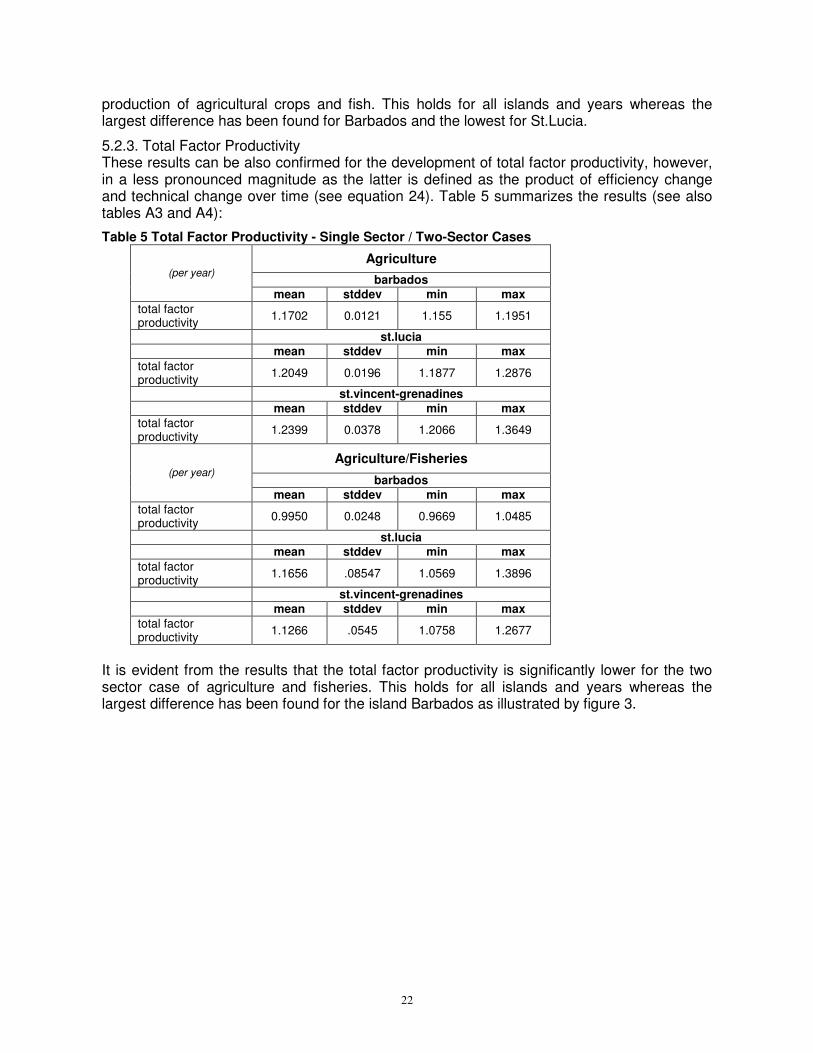
5.2.3. Total Factor Productivity These results can be also confirmed for the development of total factor productivity, however, in a less pronounced magnitude as the latter is defined as the product of efficiency change and technical change over time (see equation 24). Table 5 summarizes the results (see also tables A3 and A4):
Table 5 Total Factor Productivity - Single Sector / Two-Sector Cases
Agriculture
barbados (per year)
mean stddev min max
total factor productivity
1.1702 0.0121 1.155 1.1951
st.lucia mean stddev min max
total factor productivity
1.2049 0.0196 1.1877 1.2876
st.vincent-grenadines
mean stddev min max
total factor productivity
1.2399 0.0378 1.2066 1.3649
Agriculture/Fisheries
barbados (per year)
mean stddev min max
total factor productivity
0.9950 0.0248 0.9669 1.0485
st.lucia mean stddev min max
total factor productivity
1.1656 .08547 1.0569 1.3896
st.vincent-grenadines
mean stddev min max
total factor productivity
1.1266 .0545 1.0758 1.2677
It is evident from the results that the total factor productivity is significantly lower for the two sector case of agriculture and fisheries. This holds for all islands and years whereas the largest difference has been found for the island Barbados as illustrated by figure 3.

23
Figure 3 Total Factor Productivity - Single Sector / Two-Sector Cases
0.90
0.95
1.00
1.05
1.10
1.15
1.20
1.25
1.30
1.35
1.40
1961
1963
1965
1967
1969
1971
1973
1975
1977
1979
1981
1983
1985
1987
1989
1991
1993
1995
1997
1999
2001
2003
year
total factor
productivity
barbados (agr)
stlucia (agr)
stvincentgrenadines (agr)
barbados (agr/fish)
stlucia (agr/fish)
stvincgrenadines (agr/fish)
5.2.4. Economies of Scale and Technological Biases Significant differences in the scale efficiency have been found for the individual islands as well as cases (see appendix table A5 for detailed values). The mean scale efficiencies range from about 0.486 in the single case for St.Lucia to about 0.901 in two sector case for Barbados. Figure 4 illustrates the development over time:

24
Figure 4 Scale Efficiencies - Single Sector / Two-Sector Cases
0.00
0.10
0.20
0.30
0.40
0.50
0.60
0.70
0.80
0.90
1.00
1961
1963
1965
1967
1969
1971
1973
1975
1977
1979
1981
1983
1985
1987
1989
1991
1993
1995
1997
1999
2001
2003
2005
year
scale efficiency
barbados (agr)
stlucia (agr)
stvincentgrenadines (agr)
barbados (agr/fish)
stlucia (agr/fish)
stvincgrenadines (agr/fish)
Only in the single sector case for St.Vincent/Grenadines the scale efficiency steadily increases over time whereas a steady decline has been found for the island Barbados in both cases investigated. The development of the other scale efficiencies peak at some year during the period of the 1980s.
Table 6 summarizes the empirical evidence found for the biases in technological change over time for both cases.

25
Table 6 Technological Biases - Single Sector / Two-Sector Cases model I model II
barbados
input/output mean stddev mean stddev
tractor 0.1514 0.1615 9.5484 3.9963
fertilizer -0.0029 0.0949 -11.4463 5.4554
land 0.5157 0.1447 14.6679 6.7332
cassava 0.5964 0.1140 5.8457 3.8213
coconuts 0.0224 0.1609 -7.0829 3.0063
potatos -0.2262 0.1163 8.8801 2.9985
yams 0.0472 0.1057 6.6056 2.5852
fish - - 4.9825 2.6398 st.lucia
input/output mean stddev mean stddev
tractor 1.6429 0.0718 0.0487 0.2510
fertilizer -0.2939 0.0736 -0.1931 0.0896
land 0.9486 0.1439 -0.3004 0.2812
cassava -0.3958 0.1503 -0.7659 0.2939
coconuts 1.0014 0.0980 0.3339 0.1718
potatos -0.7561 0.1899 0.5722 0.12916
yams -0.4444 0.0609 0.0071 0.0724
fish - - 0.2682 0.1113 st.vincent-grenadines
input/output mean stddev mean stddev
tractor 1.1468 0.4338 0.0963 0.2714
fertilizer -0.1871 0.0373 -0.2836 0.1405
land 1.2156 0.5368 0.0036 0.6176
cassava 0.1281 0.1425 -0.6918 0.1818
coconuts 0.6111 0.1849 0.4023 0.1269
potatos -0.5035 0.2047 0.6567 0.2974
yams -0.2741 0.0811 0.0359 0.2187
fish - - 0.3862 0.1234
For all islands and models technological change showed to be machinery (i.e. tractor) input saving, fertilizer input wasting as well as fish output increasing at the sample mean. This implies that because of technical change over time relatively more fish has been produced by using less machinery and increasingly more fertilizer. With respect to technical change due to other inputs and outputs developments the empirical evidence is mixed over islands and models analysed.

26
5.2.5. Environmental Externalities – Environmental Efficiencies Figure 5 finally shows the differencies in total factor productivity between the two cases investigated simply calculated as the ratio of total factor productivity in the two sector to total factor productivity in the single sector case (see appendix table A6 for the individual values).
Figure 5 Single Sector / Two Sector Case – ‘Environmental Externalities’
0.60
0.70
0.80
0.90
1.00
1.10
1.20
1961
1963
1965
1967
1969
1971
1973
1975
1977
1979
1981
1983
1985
1987
1989
1991
1993
1995
1997
1999
2001
2003 year
two sector/
single sector
barbados (tfp)
st.lucia (tfp)
st.vincgren (tfp)
I becomes evident that positive externalities between agricultural production and fisheries production could be only found for St.Lucia in the 1960s. For all other years as well as other islands negative externalities between agricultural production and fisheries production have to be stated (see the 1.00 line as the threshold). The negative externalities are the largest for St.Vincent/Grenadines and the lowest for St.Lucia over all years examined. If those negative externalities are interpreted as environmental inefficiency with respect to the joint production of agricultural crops (i.e. bananas, cassava, coconuts, potatos, yams) and fish, then one can conclude that the environmental efficiency is the highest for the island St.Lucia over all years and the lowest for St.Vincent/Grenadines.
5.2.6. Inefficiency Effects – Single and Two Sector Perspectives With respect to the explanation of the variance in inefficiency over the different years we tested the island related dummies for Barbados and St.Vincent/Grenadines as well as their interaction effects with time. The choice of these inefficiency explaining factors is due to prior evidence on the regional conditions (i.e. climatic conditions or soil quality differences), efficiency related literature (see e.g. Irz/Thirtle, 2004 or Sauer et al., 2006), and discussions with regional experts. Due to the aggregate nature of our study as well as a general lack of data with respect to the focused islands, however, we were not able to include socio-economic variables, such as educational level, farming experience, extension services etc. All factors chosen showed a significant effect on single sector as well as two sectoral inefficiency.

27
Table 7 Inefficiency Effects
Factor Model I (single sector) Model II (two sector)
Location Barbados -1.2795** 3.5458***
Location St.Vincent/Grenadines 7.9944*** 2.8229***
Time x Barbados 0.1141*** -1.6297**
Time x St.Vincent/Grenadines -0.1328*** 0.0896***
*,**,***: Significance at 10, 5, and 1 % -Level.
For both models the regional location St.Vincent/Grenadines showed a highly negative effect on technical efficiency for the investigated years and products. The empirical evidence with respect to the other factors is nevertheless mixed: Whereas the regional location Barbados showed to have a positive effect on agricultural efficiency (model I), it has a significant negative effect on the joint efficiency of agricultural and fisheries production (model II). The same holds for the time and St.Vincent/Grenadines related cross term but the opposite has been found for the time and Barbados related cross term showing a negative effect on agricultural efficiency (model I) and a significant positive effect on the joint efficiency of agricultural and fisheries production (model II).
5.3. Implications for Regional Integration The preceeding quantitative analysis delivered the following results: (1) For both Barbados and St.Lucia the mean technical eficiency was found to be lower for the two sector case, however, the opposite was found for the island of St.Vincent/Grenadines. (2) It became evident that the rate of technical change is significantly lower for the two sector case of a joint production of agricultural crops and fish. This holds for all islands and years whereas the largest difference has been found for Barbados and the lowest for St.Lucia. (3) Consequently the results show that the total factor productivity is significantly lower for the two sector case which holds for all islands and years whereas the largest difference has been found for the island Barbados. (4) Only in the single sector case for St.Vincent/Grenadines the scale efficiency steadily increases over time. (5) Assuming that the negative externalities with respect to total factor productivity found can be interpreted as environmental inefficiency for the joint production of agricultural crops and fish, we conclude that the environmental efficiency is the highest for the island St.Lucia over all years and the lowest for St.Vincent/Grenadines.
With respect to the proposed economic integration in the region these findings suggest the following crucial implications with respect to an integrated (economic and environmental) perspective on rural development:
- Based on the documented negative externalities of agricultural production on fisheries for all islands, sustainable integration scenarios have to consider the relative advantages of the islands not only with respect to production but also with respect to environmental efficiency.
- As the highest and lowest negative externalities have been found for St.Vincent/Grenadines and St.Lucia respectively, a gradual dislocation of fisheries production from the island St.Vincent/Grenadines to the island St.Lucia should be considered. This means, focusing policy support on the comparative advantage of St.Lucia with respect to environmental efficiency.
- The documented scale inefficiencies further support this implication: Most recently the highest economies of scale have been found for St.Lucia (about 4.399 for the year 2005) suggesting significant economic gains by a further extension of the joint production of agricultural crops and fish on this island.

28
6 - Conclusions In a world stage of increasing regional organizations, groupings and blocs, the Caribbean region continues to investigate the feasibility of Caribbean regional integration from various perspectives. Given the geographical and oceanographic features of the Caribbean region and the general economic and environmental characteristics of Caribbean economies, the minimization of environmental degradation must be predicated on some level of regional cooperation. The traditional focus of the benefits of regional integration is on sector productivities, comparative advantages and factor specializations. However, bringing the environmental sector into the analysis from not only a “source and sink” point of view but also as the medium through which negative inter-sectoral externalities exist means that the traditional focus should be amended. The objectives of regional integration, in particular in a resource-dependent, small-island region such as the Caribbean should not be sector productivities alone but rather sector productivities together with the minimization of inter-sectoral externalities. This paper focuses on a subset of Caribbean economies and a subset of Caribbean agricultural crops. The islands of Barbados, St. Lucia and St. Vincent and the Grenadines are investigated with respect to five common and important crops – bananas, cassavas, coconuts, potatoes and yams. Within this framework, the possibility of negative externalities via land-based agricultural pollution of the marine environment is brought into the analysis by considering the joint efficiencies of agriculture and total fish production of the three countries. This analysis can be considered a template for an investigation of regional cooperation and specialization from an environmental point of view. For simplicity we have considered a subset of countries and crops in the Caribbean. This analysis can of course be extended and broadened to larger cases. The objective is to begin a demonstration of how, in policy considerations in developing countries and regions, environmental concerns can be brought to play a much larger role.

29
7 - References X Shephard (1970) Chambers (1988) Lovell et al. (1994) Battese/Coelli (1995) Aigner et al. (1977) Coelli/Perelman (1996) Sauer 2006 Sauer et al., 2006 Irz/Thirtle, 2004 Nishimuzu and Page (1982) Coelli et al. (1998) Faere et al. (1994) Wooldridge (2002) Efron 1979 Efron/Tibshirani 1993 Horowitz (2001)

30
8 - Appendices
Table A1 Bootstrapped Panel Frontier Estimates – Model I (Single Sector)
X
Table A2 Bootstrapped Panel Frontier Estimates – Model II (Two Sector)
X

31
Table A3 Efficiency, Technical Change and Total Factor Productivity – Single Sector Model
IslandIslandIslandIsland BarbadosBarbadosBarbadosBarbados StLuciaStLuciaStLuciaStLucia StVincentStVincentStVincentStVincent
YearYearYearYear Technical Technical Technical Technical
Efficiency Efficiency Efficiency Efficiency
Technical Technical Technical Technical
Efficiency Efficiency Efficiency Efficiency
ChangeChangeChangeChange
Technical Technical Technical Technical
ChangeChangeChangeChange
Total FaTotal FaTotal FaTotal Factor ctor ctor ctor
ProductivityProductivityProductivityProductivity
Technical Technical Technical Technical
Efficiency Efficiency Efficiency Efficiency
Technical Technical Technical Technical
Efficiency Efficiency Efficiency Efficiency
ChangeChangeChangeChange
Technical Technical Technical Technical
ChangeChangeChangeChange
Total Factor Total Factor Total Factor Total Factor
ProductivityProductivityProductivityProductivity
1961 0.9724 0.3193 0.1798
1962 0.9745 1.0021 1.1573 1.1597 0.3475 1.0884 1.1831 1.2876 0.2042 1.1357 1.2018 1.3649
1963 0.9763 1.0019 1.1577 1.1599 0.3758 1.0816 1.1701 1.2655 0.2297 1.1251 1.1910 1.3400
1964 0.9781 1.0018 1.1559 1.1579 0.4041 1.0753 1.1539 1.2408 0.2562 1.1153 1.1796 1.3156
1965 0.9797 1.0016 1.1540 1.1559 0.4322 1.0695 1.1535 1.2337 0.2834 1.1063 1.1797 1.3051
1966 0.9812 1.0015 1.1534 1.1552 0.4599 1.0642 1.1524 1.2263 0.3112 1.0980 1.1821 1.2979
1967 0.9825 1.0014 1.1554 1.1571 0.4872 1.0593 1.1512 1.2194 0.3393 1.0904 1.1843 1.2913
1968 0.9838 1.0013 1.1579 1.1595 0.5139 1.0548 1.1519 1.2150 0.3677 1.0835 1.1866 1.2856
1969 0.9850 1.0012 1.1551 1.1565 0.5399 1.0506 1.1537 1.2121 0.3960 1.0770 1.1851 1.2764
1970 0.9861 1.0011 1.1571 1.1584 0.5652 1.0468 1.1557 1.2098 0.4242 1.0711 1.1833 1.2674
1971 0.9871 1.0010 1.1654 1.1666 0.5896 1.0432 1.1581 1.2082 0.4520 1.0657 1.1836 1.2613
1972 0.9881 1.0010 1.1686 1.1697 0.6132 1.0400 1.1603 1.2067 0.4794 1.0607 1.1808 1.2524
1973 0.9890 1.0009 1.1643 1.1654 0.6358 1.0369 1.1615 1.2044 0.5063 1.0560 1.1775 1.2435
1974 0.9898 1.0008 1.1541 1.1550 0.6575 1.0342 1.1627 1.2024 0.5325 1.0518 1.1765 1.2374
1975 0.9905 1.0008 1.1552 1.1561 0.6783 1.0316 1.1637 1.2004 0.5580 1.0478 1.1760 1.2323
1976 0.9912 1.0007 1.1590 1.1598 0.6981 1.0292 1.1647 1.1987 0.5827 1.0442 1.1768 1.2288
1977 0.9919 1.0007 1.1601 1.1608 0.7170 1.0270 1.1630 1.1944 0.6065 1.0409 1.1805 1.2287
1978 0.9925 1.0006 1.1662 1.1669 0.7349 1.0250 1.1623 1.1913 0.6294 1.0378 1.1865 1.2313
1979 0.9930 1.0006 1.1640 1.1647 0.7519 1.0231 1.1656 1.1926 0.6514 1.0349 1.1843 1.2257
1980 0.9935 1.0005 1.1623 1.1629 0.7679 1.0214 1.1675 1.1924 0.6724 1.0323 1.1818 1.2200
1981 0.9940 1.0005 1.1599 1.1605 0.7831 1.0198 1.1677 1.1908 0.6925 1.0299 1.1850 1.2204
1982 0.9945 1.0004 1.1574 1.1579 0.7975 1.0183 1.1680 1.1894 0.7116 1.0276 1.1887 1.2216
1983 0.9949 1.0004 1.1613 1.1618 0.8110 1.0169 1.1691 1.1889 0.7298 1.0256 1.1914 1.2218
1984 0.9953 1.0004 1.1605 1.1610 0.8237 1.0157 1.1706 1.1889 0.7471 1.0236 1.1912 1.2194
1985 0.9956 1.0004 1.1628 1.1632 0.8356 1.0145 1.1707 1.1877 0.7634 1.0219 1.1899 1.2159
1986 0.9959 1.0003 1.1674 1.1678 0.8468 1.0134 1.1728 1.1885 0.7789 1.0202 1.1905 1.2146
1987 0.9962 1.0003 1.1710 1.1714 0.8573 1.0124 1.1800 1.1947 0.7934 1.0187 1.2049 1.2274
1988 0.9965 1.0003 1.1725 1.1728 0.8672 1.0115 1.1844 1.1980 0.8072 1.0173 1.2182 1.2393
1989 0.9968 1.0003 1.1727 1.1730 0.8764 1.0106 1.1863 1.1990 0.8201 1.0160 1.2156 1.2351
1990 0.9970 1.0002 1.1762 1.1765 0.8850 1.0098 1.1870 1.1987 0.8322 1.0148 1.2130 1.2310
1991 0.9972 1.0002 1.1771 1.1773 0.8930 1.0091 1.1872 1.1980 0.8437 1.0137 1.2105 1.2271
1992 0.9974 1.0002 1.1837 1.1839 0.9006 1.0084 1.1885 1.1985 0.8544 1.0127 1.2050 1.2203
1993 0.9976 1.0002 1.1852 1.1854 0.9076 1.0078 1.1885 1.1977 0.8644 1.0117 1.1998 1.2139
1994 0.9978 1.0002 1.1792 1.1794 0.9141 1.0072 1.1888 1.1973 0.8738 1.0109 1.1958 1.2088
1995 0.9980 1.0002 1.1875 1.1876 0.9202 1.0067 1.1887 1.1966 0.8826 1.0101 1.1961 1.2081
1996 0.9981 1.0002 1.1949 1.1951 0.9259 1.0062 1.1887 1.1961 0.8908 1.0093 1.1973 1.2085
1997 0.9983 1.0001 1.1919 1.1921 0.9312 1.0057 1.1884 1.1952 0.8985 1.0086 1.1965 1.2068
1998 0.9984 1.0001 1.1884 1.1885 0.9362 1.0053 1.1896 1.1959 0.9056 1.0080 1.1970 1.2066
1999 0.9985 1.0001 1.1866 1.1867 0.9408 1.0049 1.1942 1.2000 0.9123 1.0074 1.1993 1.2081
2000 0.9986 1.0001 1.1855 1.1857 0.9450 1.0045 1.1937 1.1991 0.9185 1.0068 1.2025 1.2108
2001 0.9987 1.0001 1.1844 1.1845 0.9490 1.0042 1.1922 1.1972 0.9243 1.0063 1.2061 1.2137
2002 0.9988 1.0001 1.1805 1.1806 0.9527 1.0039 1.1969 1.2016 0.9298 1.0059 1.2081 1.2152
2003 0.9989 1.0001 1.1814 1.1815 0.9561 1.0036 1.2001 1.2044 0.9348 1.0054 1.2092 1.2158
2004 0.9990 1.0001 1.1832 1.1833 0.9593 1.0033 1.2020 1.2060 0.9395 1.0050 1.2110 1.2170
2005 0.9991 1.0001 1.1831 1.1832 0.9623 1.0031 1.2026 1.2063 0.9438 1.0046 1.2157 1.2213

32
Table A4 Efficiency, Technical Change and Total Factor Productivity – Two Sector Model
IslandIslandIslandIsland BarbadosBarbadosBarbadosBarbados StLuciaStLuciaStLuciaStLucia StVincentStVincentStVincentStVincent
YearYearYearYear Technical Technical Technical Technical
Efficiency Efficiency Efficiency Efficiency
Technical Technical Technical Technical
Efficiency Efficiency Efficiency Efficiency
ChangeChangeChangeChange
Technical Technical Technical Technical
ChangeChangeChangeChange
Total Factor Total Factor Total Factor Total Factor
ProductivityProductivityProductivityProductivity
TechnTechnTechnTechnical ical ical ical
Efficiency Efficiency Efficiency Efficiency
Technical Technical Technical Technical
Efficiency Efficiency Efficiency Efficiency
ChangeChangeChangeChange
Technical Technical Technical Technical
ChangeChangeChangeChange
Total Factor Total Factor Total Factor Total Factor
ProductivityProductivityProductivityProductivity
Technical Technical Technical Technical
Efficiency Efficiency Efficiency Efficiency
Technical Technical Technical Technical
Efficiency Efficiency Efficiency Efficiency
ChangeChangeChangeChange
Technical Technical Technical Technical
ChangeChangeChangeChange
Total Factor Total Factor Total Factor Total Factor
ProductivitProductivitProductivitProductivityyyy
1961 0.9128 0.0487 0.1306
1962 0.9203 1.0082 1.0400 1.0485 0.0641 1.3168 0.9702 1.2776 0.1572 1.2036 1.0533 1.2677
1963 0.9272 1.0075 1.0373 1.0451 0.0823 1.2843 0.9682 1.2435 0.1860 1.1835 1.0501 1.2428
1964 0.9336 1.0068 1.0357 1.0428 0.1034 1.2554 1.1069 1.3896 0.2168 1.1655 1.0766 1.2548
1965 0.9394 1.0062 1.0353 1.0417 0.1271 1.2296 1.1092 1.3639 0.2492 1.1494 1.0804 1.2418
1966 0.9447 1.0057 1.0322 1.0380 0.1534 1.2067 1.1116 1.3414 0.2828 1.1349 1.0845 1.2308
1967 0.9496 1.0052 1.0291 1.0344 0.1819 1.1862 1.1133 1.3206 0.3173 1.1219 1.0831 1.2151
1968 0.9540 1.0047 1.0258 1.0306 0.2125 1.1679 1.1169 1.3045 0.3523 1.1102 1.0813 1.2004
1969 0.9581 1.0043 1.0221 1.0265 0.2447 1.1515 1.1144 1.2833 0.3874 1.0997 1.0772 1.1846
1970 0.9618 1.0039 1.0260 1.0300 0.2781 1.1368 1.1111 1.2632 0.4223 1.0902 1.0710 1.1677
1971 0.9652 1.0035 1.0115 1.0151 0.3125 1.1236 1.1089 1.2461 0.4568 1.0817 1.0726 1.1602
1972 0.9683 1.0032 1.0054 1.0086 0.3475 1.1118 1.1064 1.2301 0.4906 1.0740 1.0727 1.1521
1973 0.9711 1.0029 1.0029 1.0058 0.3826 1.1011 1.0900 1.2002 0.5235 1.0670 1.0716 1.1434
1974 0.9737 1.0027 0.9989 1.0016 0.4176 1.0915 1.0930 1.1930 0.5553 1.0607 1.0713 1.1363
1975 0.9761 1.0024 0.9949 0.9973 0.4522 1.0828 1.0936 1.1842 0.5859 1.0551 1.0688 1.1276
1976 0.9782 1.0022 0.9940 0.9962 0.4861 1.0750 1.0844 1.1657 0.6151 1.0499 1.0689 1.1222
1977 0.9802 1.0020 0.9919 0.9939 0.5191 1.0679 1.0941 1.1685 0.6429 1.0453 1.0624 1.1105
1978 0.9820 1.0018 0.9912 0.9930 0.5511 1.0616 1.0779 1.1443 0.6693 1.0411 1.0584 1.1018
1979 0.9836 1.0017 0.9923 0.9939 0.5818 1.0558 1.0874 1.1481 0.6943 1.0373 1.0708 1.1107
1980 0.9851 1.0015 0.9911 0.9926 0.6112 1.0506 1.0836 1.1384 0.7177 1.0338 1.0662 1.1022
1981 0.9864 1.0014 0.9867 0.9881 0.6393 1.0459 1.0852 1.1349 0.7398 1.0307 1.0642 1.0968
1982 0.9876 1.0012 0.9846 0.9859 0.6659 1.0416 1.0813 1.1263 0.7604 1.0278 1.0606 1.0901
1983 0.9888 1.0011 0.9844 0.9855 0.6910 1.0377 1.0711 1.1115 0.7796 1.0253 1.0617 1.0886
1984 0.9898 1.0010 0.9833 0.9843 0.7147 1.0343 1.0818 1.1188 0.7975 1.0229 1.0664 1.0909
1985 0.9907 1.0009 0.9852 0.9861 0.7369 1.0311 1.0781 1.1117 0.8141 1.0208 1.0637 1.0858
1986 0.9916 1.0008 0.9896 0.9905 0.7577 1.0282 1.0789 1.1093 0.8295 1.0189 1.0657 1.0858
1987 0.9923 1.0008 0.9881 0.9889 0.7771 1.0256 1.0865 1.1143 0.8437 1.0172 1.0576 1.0758
1988 0.9930 1.0007 0.9868 0.9875 0.7951 1.0232 1.0962 1.1217 0.8569 1.0156 1.0698 1.0865
1989 0.9936 1.0006 0.9861 0.9867 0.8119 1.0211 1.1011 1.1243 0.8690 1.0142 1.0703 1.0854
1990 0.9942 1.0006 0.9839 0.9845 0.8275 1.0192 1.0956 1.1166 0.8802 1.0129 1.0703 1.0840
1991 0.9947 1.0005 0.9817 0.9822 0.8419 1.0174 1.1048 1.1241 0.8905 1.0117 1.0829 1.0956
1992 0.9952 1.0005 0.9793 0.9797 0.8552 1.0158 1.1013 1.1187 0.9000 1.0106 1.0847 1.0963
1993 0.9957 1.0004 0.9678 0.9682 0.8675 1.0144 1.1014 1.1172 0.9087 1.0096 1.0904 1.1009
1994 0.9961 1.0004 0.9733 0.9737 0.8788 1.0130 1.0959 1.1101 0.9166 1.0088 1.0907 1.1003
1995 0.9964 1.0004 0.9756 0.9760 0.8892 1.0118 1.1022 1.1153 0.9239 1.0080 1.0955 1.1042
1996 0.9967 1.0003 0.9711 0.9714 0.8988 1.0108 1.1012 1.1131 0.9306 1.0072 1.0927 1.1006
1997 0.9970 1.0003 0.9707 0.9710 0.9075 1.0098 1.0935 1.1042 0.9367 1.0066 1.0901 1.0973
1998 0.9973 1.0003 0.9709 0.9712 0.9156 1.0089 1.0997 1.1095 0.9423 1.0060 1.0940 1.1006
1999 0.9976 1.0002 0.9731 0.9734 0.9230 1.0081 1.0969 1.1058 0.9474 1.0054 1.0885 1.0944
2000 0.9978 1.0002 0.9666 0.9669 0.9297 1.0073 1.0842 1.0922 0.9521 1.0049 1.0781 1.0834
2001 0.9980 1.0002 0.9670 0.9672 0.9359 1.0067 1.0828 1.0900 0.9564 1.0045 1.0841 1.0890
2002 0.9982 1.0002 0.9678 0.9680 0.9416 1.0061 1.0785 1.0850 0.9603 1.0041 1.0868 1.0912
2003 0.9983 1.0002 0.9708 0.9709 0.9468 1.0055 1.0717 1.0776 0.9638 1.0037 1.0923 1.0964
2004 0.9985 1.0002 0.9679 0.9680 0.9515 1.0050 1.0638 1.0691 0.9671 1.0034 1.0868 1.0905
2005 0.9986 1.0001 0.9702 0.9703 0.9558 1.0045 1.0521 1.0569 0.9700 1.0031 1.0818 1.0851

33
Table A5 Scale Efficiencies - Single Sector / Two-Sector Cases
AgricultureAgricultureAgricultureAgriculture Agriculture and FisAgriculture and FisAgriculture and FisAgriculture and Fisheriesheriesheriesheries
BarbadosBarbadosBarbadosBarbados StLuciaStLuciaStLuciaStLucia StVincentStVincentStVincentStVincent BarbadosBarbadosBarbadosBarbados StLuciaStLuciaStLuciaStLucia StVincentStVincentStVincentStVincent
yearyearyearyear Scale EfficiencyScale EfficiencyScale EfficiencyScale Efficiency
1961 0.97494 0.34426 0.18003 0.95075 0.05854 0.14302
1962 0.97131 0.37556 0.20447 0.93644 0.07780 0.17291
1963 0.96780 0.40717 0.23006 0.92269 0.10087 0.20560
1964 0.96438 0.43892 0.25658 0.90943 0.12790 0.24080
1965 0.96105 0.47064 0.28387 0.89656 0.15892 0.27820
1966 0.95779 0.50218 0.31171 0.88401 0.19389 0.31744
1967 0.95459 0.53342 0.33992 0.87172 0.23268 0.35817
1968 0.95145 0.56422 0.36830 0.85962 0.27506 0.40002
1969 0.94835 0.59451 0.39670 0.84765 0.32079 0.44266
1970 0.94528 0.62418 0.42493 0.83577 0.36958 0.48577
1971 0.94224 0.65318 0.45287 0.82393 0.42112 0.52908
1972 0.93921 0.68146 0.48037 0.81208 0.47511 0.57233
1973 0.93620 0.70896 0.50732 0.80019 0.53126 0.61534
1974 0.93319 0.73566 0.53362 0.78823 0.58930 0.65792
1975 0.93018 0.76156 0.55919 0.77615 0.64900 0.69996
1976 0.92716 0.78663 0.58396 0.76394 0.71019 0.74136
1977 0.92412 0.81088 0.60787 0.75157 0.77272 0.78207
1978 0.92106 0.83433 0.63088 0.73901 0.83650 0.82206
1979 0.91798 0.85699 0.65297 0.72624 0.90150 0.86135
1980 0.91487 0.87889 0.67411 0.71324 0.96773 0.89997
1981 0.91171 0.90004 0.69430 0.70001 0.96594 0.93796
1982 0.90852 0.92049 0.71354 0.68651 0.90561 0.97540
1983 0.90529 0.94026 0.73184 0.67275 0.85122 0.98777
1984 0.90200 0.95939 0.74920 0.65871 0.80182 0.95328
1985 0.89866 0.97793 0.76564 0.64439 0.75663 0.92131
1986 0.89526 0.99590 0.78120 0.62978 0.71502 0.89150
1987 0.89180 0.98681 0.79589 0.61489 0.67645 0.86352
1988 0.88828 0.97054 0.80974 0.59970 0.64049 0.83711
1989 0.88468 0.95520 0.82279 0.58422 0.60677 0.81203
1990 0.88101 0.94067 0.83507 0.56847 0.57498 0.78808
1991 0.87727 0.92689 0.84661 0.55244 0.54486 0.76508
1992 0.87345 0.91375 0.85745 0.53614 0.51620 0.74288
1993 0.86955 0.90120 0.86762 0.51960 0.48883 0.72135
1994 0.86555 0.88916 0.87715 0.50282 0.46259 0.70037
1995 0.86147 0.87758 0.88607 0.48583 0.43737 0.67985
1996 0.85730 0.86641 0.89443 0.46864 0.41307 0.65969
1997 0.85304 0.85559 0.90225 0.45128 0.38960 0.63984
1998 0.84867 0.84509 0.90956 0.43377 0.36692 0.62022
1999 0.84421 0.83486 0.91640 0.41615 0.34496 0.60078
2000 0.83964 0.82486 0.92279 0.39844 0.32370 0.58149
2001 0.83496 0.81507 0.92875 0.38068 0.30311 0.56229
2002 0.83018 0.80545 0.93433 0.36291 0.28318 0.54318
2003 0.82528 0.79597 0.93953 0.34517 0.26390 0.52412
2004 0.82027 0.78662 0.94439 0.32749 0.24526 0.50510
2005 0.81514 0.77736 0.94893 0.30992 0.22728 0.48612

34
Table A6 Differencies in Efficiency, Technical Change and Total Factor Productivity
BarbadosBarbadosBarbadosBarbados StLuciaStLuciaStLuciaStLucia StVincentStVincentStVincentStVincent
Technical Technical Technical Technical
Efficiency Efficiency Efficiency Efficiency
Technical Technical Technical Technical
Efficiency Efficiency Efficiency Efficiency
ChangeChangeChangeChange
Technical Technical Technical Technical
ChangeChangeChangeChange
Total Factor Total Factor Total Factor Total Factor
ProductivityProductivityProductivityProductivity
TechnTechnTechnTechnical ical ical ical
Efficiency Efficiency Efficiency Efficiency
Technical Technical Technical Technical
Efficiency Efficiency Efficiency Efficiency
ChangeChangeChangeChange
Technical Technical Technical Technical
ChangeChangeChangeChange
Total Factor Total Factor Total Factor Total Factor
ProductiProductiProductiProductivityvityvityvity
Technical Technical Technical Technical
Efficiency Efficiency Efficiency Efficiency
Technical Technical Technical Technical
Efficiency Efficiency Efficiency Efficiency
ChangeChangeChangeChange
Technical Technical Technical Technical
ChangeChangeChangeChange
Total Factor Total Factor Total Factor Total Factor
ProductivityProductivityProductivityProductivity
1961 0.93870 0.15248 0.72646
1962 0.94447 1.00615 0.89863 0.90415 0.18449 1.20993 0.82002 0.99217 0.76988 1.06534 0.68233 0.72691
1963 0.94973 1.00557 0.89607 0.90106 0.21907 1.18743 0.82748 0.98258 0.80986 1.05544 0.69476 0.73328
1964 0.95452 1.00504 0.89608 0.90060 0.25576 1.16746 0.95927 1.11991 0.84632 1.04680 0.81320 0.85126
1965 0.95888 1.00457 0.89714 0.90123 0.29405 1.14971 0.96156 1.10552 0.87928 1.03926 0.81508 0.84708
1966 0.96284 1.00413 0.89488 0.89858 0.33343 1.13392 0.96464 1.09382 0.90880 1.03269 0.81607 0.84274
1967 0.96644 1.00374 0.89067 0.89400 0.37339 1.11984 0.96711 1.08300 0.93501 1.02696 0.81664 0.83866
1968 0.96971 1.00338 0.88586 0.88885 0.41345 1.10728 0.96964 1.07367 0.95810 1.02199 0.81715 0.83512
1969 0.97267 1.00306 0.88482 0.88753 0.45316 1.09606 0.96599 1.05878 0.97826 1.01767 0.81514 0.82954
1970 0.97536 1.00276 0.88672 0.88916 0.49215 1.08604 0.96139 1.04411 0.99570 1.01393 0.81249 0.82380
1971 0.97779 1.00249 0.86798 0.87014 0.53008 1.07707 0.95757 1.03137 1.01065 1.01069 0.80903 0.81768
1972 0.97999 1.00225 0.86030 0.86224 0.56668 1.06905 0.95356 1.01940 1.02333 1.00791 0.80754 0.81393
1973 0.98198 1.00203 0.86132 0.86307 0.60174 1.06186 0.93841 0.99646 1.03397 1.00551 0.79694 0.80133
1974 0.98379 1.00184 0.86556 0.86714 0.63509 1.05542 0.94006 0.99216 1.04277 1.00347 0.79902 0.80179
1975 0.98542 1.00166 0.86119 0.86261 0.66663 1.04966 0.93979 0.98645 1.04994 1.00173 0.79914 0.80052
1976 0.98689 1.00149 0.85764 0.85892 0.69628 1.04448 0.93103 0.97245 1.05567 1.00025 0.79119 0.79138
1977 0.98822 1.00135 0.85507 0.85622 0.72402 1.03984 0.94082 0.97830 1.06012 0.99901 0.79697 0.79618
1978 0.98942 1.00121 0.84996 0.85099 0.74985 1.03568 0.92743 0.96053 1.06346 0.99797 0.78168 0.78009
1979 0.99050 1.00109 0.85247 0.85341 0.77381 1.03195 0.93288 0.96268 1.06584 0.99711 0.78769 0.78541
1980 0.99148 1.00099 0.85273 0.85357 0.79594 1.02860 0.92814 0.95468 1.06739 0.99641 0.78537 0.78255
1981 0.99236 1.00089 0.85070 0.85145 0.81631 1.02559 0.92928 0.95306 1.06822 0.99584 0.78423 0.78097
1982 0.99315 1.00080 0.85073 0.85141 0.83499 1.02289 0.92577 0.94696 1.06845 0.99539 0.77878 0.77519
1983 0.99386 1.00072 0.84767 0.84828 0.85209 1.02047 0.91611 0.93487 1.06816 0.99505 0.76897 0.76516
1984 0.99450 1.00065 0.84729 0.84783 0.86768 1.01830 0.92415 0.94107 1.06744 0.99479 0.77579 0.77175
1985 0.99508 1.00058 0.84726 0.84775 0.88187 1.01635 0.92091 0.93597 1.06637 0.99461 0.77396 0.76979
1986 0.99560 1.00052 0.84774 0.84818 0.89475 1.01460 0.91991 0.93334 1.06500 0.99449 0.77270 0.76845
1987 0.99607 1.00047 0.84382 0.84422 0.90641 1.01304 0.92072 0.93272 1.06340 0.99443 0.76418 0.75992
1988 0.99649 1.00042 0.84164 0.84199 0.91695 1.01163 0.92557 0.93633 1.06162 0.99442 0.75980 0.75556
1989 0.99687 1.00038 0.84090 0.84121 0.92646 1.01037 0.92813 0.93775 1.05969 0.99444 0.76350 0.75926
1990 0.99721 1.00034 0.83648 0.83676 0.93502 1.00924 0.92297 0.93150 1.05766 0.99450 0.76089 0.75671
1991 0.99751 1.00031 0.83399 0.83425 0.94271 1.00823 0.93062 0.93827 1.05555 0.99459 0.76878 0.76462
1992 0.99779 1.00027 0.82731 0.82754 0.94961 1.00732 0.92662 0.93340 1.05339 0.99470 0.76898 0.76490
1993 0.99803 1.00025 0.81655 0.81675 0.95579 1.00651 0.92676 0.93279 1.05121 0.99482 0.77240 0.76841
1994 0.99825 1.00022 0.82544 0.82562 0.96132 1.00578 0.92185 0.92718 1.04903 0.99497 0.77090 0.76702
1995 0.99845 1.00020 0.82161 0.82177 0.96625 1.00513 0.92723 0.93199 1.04685 0.99512 0.77521 0.77142
1996 0.99862 1.00018 0.81266 0.81280 0.97064 1.00455 0.92638 0.93059 1.04470 0.99528 0.77370 0.77005
1997 0.99878 1.00016 0.81437 0.81450 0.97455 1.00403 0.92017 0.92388 1.04259 0.99545 0.76908 0.76558
1998 0.99892 1.00014 0.81700 0.81711 0.97802 1.00356 0.92448 0.92777 1.04052 0.99562 0.77232 0.76895
1999 0.99905 1.00013 0.82013 0.82023 0.98110 1.00315 0.91857 0.92146 1.03851 0.99580 0.76593 0.76271
2000 0.99916 1.00011 0.81537 0.81546 0.98383 1.00278 0.90832 0.91084 1.03655 0.99597 0.75533 0.75229
2001 0.99926 1.00010 0.81646 0.81654 0.98623 1.00245 0.90824 0.91047 1.03465 0.99615 0.75303 0.75013
2002 0.99935 1.00009 0.81988 0.81995 0.98836 1.00215 0.90108 0.90302 1.03282 0.99632 0.74587 0.74313
2003 0.99943 1.00008 0.82168 0.82175 0.99022 1.00189 0.89302 0.89471 1.03106 0.99649 0.73852 0.73593
2004 0.99950 1.00007 0.81804 0.81810 0.99187 1.00166 0.88502 0.88648 1.02936 0.99666 0.73084 0.72840
2005 0.99956 1.00006 0.82002 0.82007 0.99330 1.00145 0.87487 0.87613 1.02774 0.99682 0.71966 0.71738