agn spectroscopy - university of alaska systemrbseu.uaa.alaska.edu/projects/agn/agn...

AGN Spectroscopy 1

AGN SpectroscopyNature’s Most Powerful “Monsters”

Rev 5/1/08

The 2.1-meter telescope at Kitt Peak National Observatory in Arizona.

The 3-meter telescope at Lick Observatory in California.

The 3.5-meter telescope at Apache Point Observatory in New Mexico.

Travis A. Rector and Brenda A. WolpaThe National Optical Astronomy Observatory950 N. Cherry Ave., Tucson, AZ 85719 USA

email: [email protected]

Teaching NotesA Note From The Authors

The goal of this project is to search for, and to study, “active galaxies.” These are galaxies that contain a luminous source of energy called an “active galactic nucleus” (AGN). The spectroscopy obtained for this project will be used to identify whether or not an object is an AGN, and what kind. We will also use spectroscopy to determine the physical characteristics (e.g., redshift, distance and luminosity) of each object. The radio properties of objects within the FIRST survey can also be studied.

Please note that it is assumed that the instructor and students are familiar with the concepts of spectroscopy as it is used in astronomy. This document is an incomplete source of information on these topics, so further study is encouraged. In particular, the “Stellar Spectroscopy” activity will be useful for learning how to analyze an optical spectrum of a star.

This is a research project; and as such the “answers” are not known. This project is challinging. It can be difficult to determine redshifts for many of the spectra, especially the BL Lac objects. Determining redshifts of BL Lacs should prob-ably be attempted only by advanced students who already have experience with the other classes of objects.

Note: You are strongly advised to do the “stellar spectroscopy” activity first to aquaint yourself with astronomical spectra.

Prerequisites

To be able to do this research project, students should first have a basic under-standing of the following concepts:

• Spectroscopy in astronomy • Redshift and Hubble’s Law • Flux density, distance and luminosity relation (the “inverse-square” law) • Galaxies, active galaxies and quasars

Description of the Data

Much of the spectra were obtained with the 2.1-meter telescope at Kitt Peak National Observatory, located about 40 miles west of Tucson, Arizona. Spec-tra were also obtained with the 3-meter telescope at Lick Observatory and the 3.5-meter telescope at Apache Point Observatory. These spectra cover the entire optical spectrum (what we can see with our eyes). Note that these data are real;

2 AGN Spectroscopy Rev. 5/1/08

and there are occasionally defects in a spectrum. In particular, the data near both ends of a spectrum is typically much noisier than the rest of the spectrum.

Object Names

The objects you will be studying have names which must seem very unusual, but they serve a purpose. The prefix (usually a 1 to 3 letter or number code) indicates the catalog to which the object belongs. The suffix, usually a six to ten number combination (which astronomers jokingly refer to as the object’s “telephone number”), roughly gives the location of the object in the sky. For example, the name of the quasar in the first tutorial is “BQ 0740+2537”. The “BQ” prefix indicates that it is an object in the FIRST Bright Quasar Survey (see below). It is has a right ascention of approximately 07 hours, 40 minutes and a declination of +25 degrees and 37 arcminutes (in the filename “bq0740p2537” the “p” is for “plus”). These names, while somewhat confusing, help astronomers keep track of the millions of astronomical objects known.

The Research Projects

Data are available for four research projects:

The goal of the first project is to identify objects in the FIRST Bright Quasar Survey. They were discovered by the FIRST survey, an acronym for “Faint Images of the Radio Sky at Twenty-centimeters”. It is a radio survey of a por-tion of the sky with the Very Large Array (VLA) radio telescope in New Mexico. Assembled by Dr. Sally Laurent-Muehleisen at the Lawrence Livermore National Laboratory, this catalog contains objects which emit radio waves. Over 2000 spectra are available to study. The radio properties of these sources can also be studied. The tutorial for the quasar “BQ 0713+3656” shows how.

The second project consists of a spectroscopic study of FIRST radio sources that have a flat radio spectrum. These objects were selectively chosen because they are predominantly “flat-spectrum radio quasars” (FSRQs) and BL Lac objects (which are collectively known as “blazars”). However, other objects are also present in this survey, including elliptical galaxies, starburst galaxies, and perhaps other types of AGN. Spectra of 151 objects from the FIRST survey are available and are labeled with the prefix “FFS”. (Note: Currently these spectra are only in Graphical Analysis 2 format. They cannot be opened with GA 3.)

The goal of the third project is to search for quasars in the Green Bank 6cm (GB6) catalog of radio sources. This project was initiated by Dr. Jane Dennet-Thorpe at the Rijksuniversiteit Gröningen and by Dr. Rector. Currently spectra of 17 objects are available for analysis. These objects should be analyzed in the same way as the FIRST sources, although we expect most of the objects to be quasars. They are labeled with the prefix “GB” or “GB6”. (Note: Currently these spectra are only in Graphical Analysis 2 format. They cannot be opened with GA 3.)

The fourth project is to study BL Lac objects from the ROSAT-Green Bank catalog (RGB). Discovered by Dr. Sally Laurent-Muehleisen, these are BL Lacs which are in both the ROSAT and Green Bank 6cm sky surveys. The goal is to determine redshifts for these objects. It is a very difficult project and should not be attempted without first gaining experience with the previous projects. (Note: Currently these spectra are only in Graphical Analysis 2 format. They cannot be opened with GA 3.)

In addition to the research data, example spectra have been included so that

The center of the Very Large Array (VLA). The VLA is a radio telescope in New Mexico operated by the National Radio Astronomy Observatory.

The Röntgen Satellite (ROSAT) was an X-ray observatory devel-oped through a cooperative program between Germany, the United States, and the United Kingdom. The satellite was designed and operated by Ger-many, and was launched by the United States on June 1, 1990. It was turned off on February 12, 1999.

AGN Spectroscopy 3

students can follow the examples provided. Spectra for different classes of objects are also included for comparison; e.g., a composite quasar spectrum is also included courtesy of Dr. Paul Francis, Australian National University.

About the Software

This research project is designed for Graphical Analysis by Vernier Software. Graphical Analysis 3 (GA3) was chosen because it is an inexpensive software package that has the necessary analysis tools. As of this writing, 3.4 is the latest version of GA3. However, many of the spectra are still in GA v2.0 and cannot be opened by v3.0 and higher. We are in the process of converting most of the spectra to the GA3 format.

An “ì” icon appears when analysis of the data with the computer is neces-sary. Here we use the Macintosh version of Graphical Analysis to illustrate the examples, but the Windows version is identical. To order Graphical Analysis, Vernier Software can be reached at the following address:

Vernier Software, Inc. 8565 S.W. Beaverton-Hillsdale Hwy. Portland, Oregon 97225-2429 Phone: (503) 297-5317, Fax: (503) 297-1760 email: [email protected] WWW: http://www.vernier.com/

Analyzing FIRST radio images requires ImageJ, a JAVA implementation of the popular program NIH Image. ImageJ runs on many platforms, including Macintosh OS 9 and OS X as well as on Microsoft Windows and LINUX on the PC. ImageJ is free and can be found online at http://rsb.info.nih.gov/ij/

Using Graphical AnalysisSummary of Commands

GA3 has many tools that are useful for this project. Below is a brief summary of some of the commands. It is not a complete summary of all of the commands.

File/Open... (ü-O)

Opens the spectrum. Each spectrum covers roughly 4000 to 9000Å. Note that this command can only be used to open spectra in GA3 format. GA3 cannot open spectra in GA2 format or earlier.

File/Import From Text File...

Use this command to import spectra that are in text format, e.g., the FIRST Bright Quasar Survey spectra. For this command to work properly the spectral data must be comma-delimited.

Analyze/Examine (ü-E)

Activates the examine tool (the magnifying glass) which gives the wavelength (the X value) and the flux density per unit wavelength (the Y value) of the data-point closest to the cursor. It is used to determine the wavelength of emission and absorption lines in the spectrum (see illustration in the sidebar).

Analyze/Integral

Sums the area under the spectrum to give the total flux density over the spectral region selected by the cursor. This is used to measure the amount of total flux

Use the examine tool (using Analyze/Examine or ü-E) to determine the wavelength of emission and absorption lines present (the X value). The infor-mation box, which is normally in the upper left corner of the plot is shown at the top. In this example the wavelength of the emission line is 6380 Angstroms (Å). The flux density per unit wavelength is 1.456 x 10-16 erg cm-2 s-1 Å-1.

The integrate tool (Analyze/Integral) is used to sum the flux over the selected range of the spectrum. The total flux density is shown on top. In this example the total flux is 1.251 x 10-13 erg cm-2 s-1 from 6000Å to 7000Å.


density in the selected region, a step in determining an object’s luminosity.

Analyze/Statistics

Gives statistical information for the spectral region selected by the cursor, including maximum and minimum datapoint values as well as the mean, median and number of data points. This tool is useful for determining the CaII break strength.

Options/Graph Options...

The graph options window (as shown below) is used to turn off the point protectors after a spectrum is loaded from a text file. The axes options window is also useful for rescaling the X- and Y-axes by inputting ranges manually or automatically by using the data values. Note that you must first select the graph (i.e., click on it) for this option to be available in the menu.

Data/Column Options

The column options is used to adjust the displayed precision of the data. Sometimes upon loading the data values in column 2 (the flux density column) are shown as zeros because the displayed precision is not correctly set. Set the displayed preci-sion to 4 significant figures as shown below before using the examine tool.

AGN Spectroscopy 5


Rev 5/1/08

Quasars, Blazars and BL Lacs: Extreme Astronomy at the Beginning of TimeA Personal Perspective by Jeffrey F. Lockwood

Where do we come from? How did we get here? When did the Universe begin? In astronomy, these basic questions remain tantalizing in their mystery, and shrouded in cosmic doubt. Some of the astronomers who choose to investigate these mysteries select nature’s most spectacular creations to study; objects so powerful in their outpouring of energy that the most amazing fact about them is that they exist at all. These objects called quasars (originally an acronym for quasi-stellar radio sources), are billions of light years away and represent a visual time capsule of what the Universe was like when it was young. In fact, tonight at the National Science Foundations’ 2.1-meter telescope on Kitt Peak, Dr. Travis Rector will be studying objects that resemble what our galaxy the Milky Way may have looked like billions of years ago.

The KPNO 2.1-meter Telescope

I met Travis at the Visitor’s Center at Kitt Peak at 3 O’clock one Saturday afternoon. It was his third night of a four night observation run and he looked a little weary having had only 5 hours of sleep before rising three hours ago. At 4 o’clock, we went over to the telescope to begin the long process of preparing the telescope and its camera to take data. As Travis begins explaining the workings of the “Goldcam,” the spectrograph which will take the spectra of his target objects during his observing run, three visitors stare at us through the glass partition. Travis decides to invite them in and proceeds to give them an explanation of his research project, shows them the control room, and the primary mirror. They, needless to say, were immensely pleased. More satisfied taxpayers.

The Goldcam, a workhorse optical spectrograph, has evolved over the years to its present condition. Attached at the Cassegrain focus of the telescope, there are a dozen different metal boxes and cylinders protruding from the main axis of the instrument. A couple of the boxes are TV cameras; two of the cylinders are lamps used to calibrate the instrument and the data display. Some of the attachments are relics of previous incarnations of the spectrograph that are not removed so as not to compromise the balance of the telescope. It takes two technicians three hours to mount Goldcam on the end of the telescope.

The heart of the spectrograph is the diffraction grating at the very bottom of the Goldcam. It is a reflection grating with medium resolution that allows a broad range of optical wavelengths to be studied (3500 to 8000 Å), covering the entire visible spectrum as well as parts of the near infrared and near UV. When studying AGN (active galactic nuclei), astronomers like to have coverage over as much of the spectrum as possible to detect the emission lines common in such objects, which may be at any wavelength.

The light from the AGN being studied is reflected several times before it gives

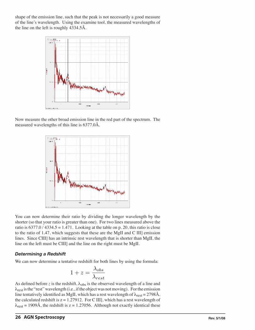
The GoldCam spectrograph, attached to the bottom of the 2.1-meter telescope.

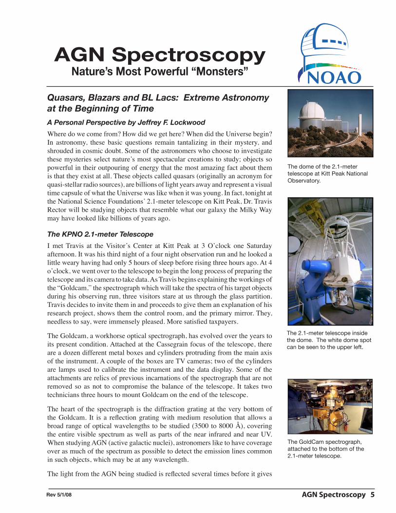
The dome of the 2.1-meter telescope at Kitt Peak National Observatory.

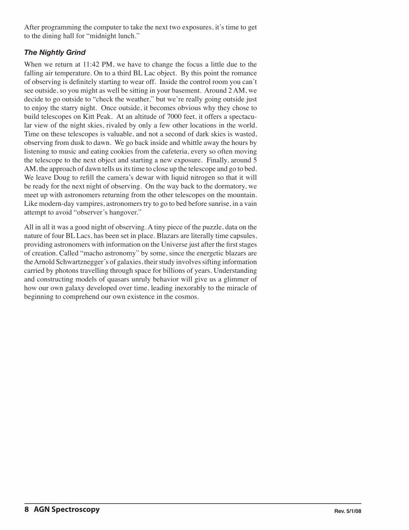
The 2.1-meter telescope inside the dome. The white dome spot can be seen to the upper left.


The 2.1-meter telescope at sunset.

up its secrets to the astronomer. Bouncing off the 2.1 meter primary mirror then off of the convex secondary and through the back of the telescope, the light hits a silvered plate at the focal plane of the telescope that has a 160 µm slit cut in it. A small video camera uses reflected light from the plate to see the slit, allow-ing the telescope operator to center objects on it during the night. After passing through the slit, the light travels down the axis of the camera and is reflected from the grating at the bottom back up to a flat mirror, which passes the spectrum to the CCD camera. The CCD chip is rectangular (3,096 X 512 pixels) to display the spectral lines over a wide range of frequency space. The whole camera is cooled by liquid nitrogen to reduce “noise” and thereby improve its sensitivity. To keep it cold during the entire night, the camera is enclosed in a device called a dewar, which acts much like a thermos bottle. Then the spectrum is sent to the computer where it is displayed on a monitor. A software package translates the image to a graphical representation that looks a lot like a seismic record of the San Francisco earthquake.

At 4:20 PM, Travis starts to calibrate the CCD array. To equalize the response of each pixel in the array, pictures of a flat white spot affixed to the dome are taken and divided into the signal of each pixel. This procedure is accomplished by taking fifty 5-second exposures and averaging them. Then, as a double check and to fine tune the response of the blue end of the spectrum, a quartz lamp that is mounted on the Goldcam is turned on and illuminates the chip. Usually, fifty exposures of 8 seconds are taken with the quartz lamp to finish the flat fielding process. Travis then inserts a cassette-size Exabyte tape to store his data for the night. With a capacity of 4 GB, he can place all of his data for a four day observing run on it with ease. At 5:30 PM, we decide it’s time for dinner.

Waiting for Nightfall

After eating, we walked back up to the telescope and asked Doug Williams, our telescope operator for the night, to open the door to the catwalk so we can watch the sunset. This is a ritual for many astronomers, to take time out to appreciate the beauty and tranquility of the setting sun and the approach of darkness despite the mounting pressures in preparing for the hectic night of observing.

At 7:00 PM, Doug centers a 7.5 magnitude SAO star and calculates the “seeing” (the smallest object, diameter measured in seconds of arc, that the telescope can resolve at that moment) with a new computer program. He says, “Pretty good, 1.2 arcseconds.” Evidently, even though the skies were pretty free of clouds, the seeing was poor last night, forcing him to only take data on the brightest objects in his observing list. At 7:15 PM, Travis begins a half-hour process of focusing the camera. He takes seven 10-second exposures of a standard star’s spectra and displays all of them on the monitor to find the clearest and most distinct image. He repeats the process and settles on a focus of 2650 (mm per focus unit) and Doug adjusts the secondary mirror accordingly.

Doug selects another standard star, a white dwarf this time so a final test expo-sure can be taken. As the telescope slews slowly towards its position in the sky, stars on the monitor whip by like meteors. Once the star is centered on the slit four two minute exposures are taken. The computer then calculates a sensitivity function that will calibrate the chips response across the continuum to match the star’s spectrum, particularly in the blue portion.

Doug has been a telescope operator for one year. Prior to coming to Kitt Peak, he spent 15 years as a fisherman in Alaska. For five months each year, he would

Dr. Travis Rector standing next to the 2.1-meter telescope on Kitt Peak.

AGN Spectroscopy 7

An illustration of what an AGN is believed to look like. At the very center is a massive Black Hole which is pulling in stars, gas and dust (the surrounding torus). Nearby gas clouds (the black and white dots) are heated and produce emission lines. Some AGN eject jets of gas which shoot away at nearly the speed of light.

work on a salmon or herring boat and earn enough money to support himself the rest of the year. Then, each winter he would take courses at the University of Washington. Once Doug graduated with a degree in physics, he decided to find a second job to supplement his fishing income so he applied for and was hired for the operator’s job last year.

At 7:55 PM, Travis turns on the HeNeAr lamp that is a light source filled with Helium, Neon, and Argon gas. The lamp is attached to the spectrograph and illuminates the CCD s that it can be used to calibrate the wavelength scale of the camera. At 8:00 PM, we are finally ready to begin the actual data-taking phase. Travis gives Doug a BL Lac object from his “cache,” a list of 40 or 50 research targets he has supplied to the operator. He figures we will have time to take data on three or four BL Lacs from his list. He needs to take four 30 minute exposures of each object. All four are later averaged for the most accurate spectrum possible. Travis is working with Dr. Sally Laurent-Mueheleisen from Lawrence Livermore Lab and his former advisor, Dr. John Stocke from the University of Colorado on this project. He will be taking much of the data over the course of the spring and summer. The purpose of the study is to survey the entire range of BL Lac objects, from high to low energy.

Mother Nature’s “Monsters”

BL Lacs are related to quasars. Specifically, just to confuse things, they are also related to objects called “flat-spectrum radio quasars” (FSRQs). Collectively, they are known as “blazars,” a word that comes from the combination of the terms BL Lac and quasar. It appears that blazars are oriented such that their “jets,” enormous outpourings of electrons and protons from the black hole, are coming straight at us. The jets, travelling at nearly the speed of light, are ejected along the axis of rotation of the black hole. The particles in the jets are affected by time dilation which “stacks up” their incoming wavefronts to the point where it appears that the energy coming from the BL Lac is as much as a thousand times greater than it really is. The process is called “Doppler boosting.” Because the jet is so bright, it tends to overwhelm any emission from the rest of the galaxy, washing out any emission or absorption lines that might be there. For this reason, BL Lac spectra are not easy to interpret. The main thrust of the research project is the study of unification models for the different varieties of blazars. The major questions is: How are all these different types of objects related? Is it: 1) Orientation: Do they look different because we see each object from a different direction? 2) Environment: Are they in clusters of galaxies or are they alone? 3) Evolution: How do they change over time? And 4) Intrinsic physical properties: Are they just different? About the size of our solar system, all blazars seem to have a huge black hole powering them, with a mass equal to over 10 million suns. The gas near the black hole yields the emission lines seen in their spectra.

At 8:30 PM, the first 30-minute exposure is done. The data is displayed on the computer screen. The spectrum doesn’t look like much as it is a black and white display of the BL Lac’s continuous spectrum, with a few bumps and lines here and there. Later, Travis will use the computer to transform the raw data into a graphical form that is much easier to interpret. Observing is a continual process of “hurry up and wait.” It’s grind it out time, the non-romantic, repetitive push-a-button-and-watch-the-clock-for-30-minutes time.

At 10 PM we’re finished with the first object. Before going to a second one, Travis uses the HeNeAr lamp to recalibrate the camera. Doug checks the temperature to see if the focus of the telescope might have changed during the observation.


After programming the computer to take the next two exposures, it’s time to get to the dining hall for “midnight lunch.”

The Nightly Grind

When we return at 11:42 PM, we have to change the focus a little due to the falling air temperature. On to a third BL Lac object. By this point the romance of observing is definitely starting to wear off. Inside the control room you can’t see outside, so you might as well be sitting in your basement. Around 2 AM, we decide to go outside to “check the weather,” but we’re really going outside just to enjoy the starry night. Once outside, it becomes obvious why they chose to build telescopes on Kitt Peak. At an altitude of 7000 feet, it offers a spectacu-lar view of the night skies, rivaled by only a few other locations in the world.Time on these telescopes is valuable, and not a second of dark skies is wasted, observing from dusk to dawn. We go back inside and whittle away the hours by listening to music and eating cookies from the cafeteria, every so often moving the telescope to the next object and starting a new exposure. Finally, around 5 AM, the approach of dawn tells us its time to close up the telescope and go to bed. We leave Doug to refill the camera’s dewar with liquid nitrogen so that it will be ready for the next night of observing. On the way back to the dormatory, we meet up with astronomers returning from the other telescopes on the mountain. Like modern-day vampires, astronomers try to go to bed before sunrise, in a vain attempt to avoid “observer’s hangover.”

All in all it was a good night of observing. A tiny piece of the puzzle, data on the nature of four BL Lacs, has been set in place. Blazars are literally time capsules, providing astronomers with information on the Universe just after the first stages of creation. Called “macho astronomy” by some, since the energetic blazars are the Arnold Schwartznegger’s of galaxies, their study involves sifting information carried by photons travelling through space for billions of years. Understanding and constructing models of quasars unruly behavior will give us a glimmer of how our own galaxy developed over time, leading inexorably to the miracle of beginning to comprehend our own existence in the cosmos.

AGN Spectroscopy 9


Rev 5/1/08

IntroductionThe Power of Spectroscopy

Spectroscopy is the study of “what kinds” of light we see from an object. It is a measure of the quantity of each color of light (or more specifically, the amount of each wavelength of light). It is a powerful tool in astronomy. In fact, most of what we know in astronomy is due to spectroscopy: it can reveal the temperature, velocity and composition of an object as well as be used to infer mass, distance and many other pieces of information. Spectroscopy is done at all wavelengths of the electromagnetic spectrum, from radio waves to gamma rays; but here we will focus on optical light.

The three types of spectra are shown in the diagram below: continuous, emis-sion line and absorption line. A continuous spectrum includes all wavelengths of light; i.e., it shows all the colors of the rainbow (case “a” in the diagram below). It is produced by a dense object that is hot and dense, either a dense gas (such as a star) or a liquid or solid (e.g., a tungsten filament in a light bulb). In contrast, an emission line spectrum consists of light at only a few wavelengths, i.e., at only a few discrete colors (case “b”). An emission line spectrum is produced by a hot, tenuous (low-density) gas. Importantly, the wavelengths of the emission lines depend on the type of gas; e.g., hydrogen gas produces different emission lines than helium. Absorption lines can be best thought of as the opposite of emission lines. While an emission line adds light of a particular wavelength, an absorption line subtracts light of a particular wavelength. Again opposite of emission lines, absorption lines are produced by a cool gas. Since there must be some light to subtract, absorption lines can only be seen when superimposed onto a continuum spectrum. Thus, for absorption lines to be seen, cool gas must lie between the viewer and a hot source (case “c”). The cool gas absorbs light from the hot source before it gets to the viewer. Here “hot” and “cool” are relative terms- the gas must simply be cooler than the continuum source. Also note that a gas absorbs the same wavelengths of light that it emits.

Astronomers like to plot spectra differently than you often see in a textbook. Spectra are plotted as flux (the amount of light) as a function of wavelength. In the diagram above the three types of spectra are shown. In the bottom frame they are shown together, as they might appear in an object’s spectrum.

Emission and absorption lines are named after the element responsible for the line (remember that different types of gas produce different lines) and the gas’ ionization state. Atoms in a hot gas can lose electrons, either by absorbing pho-


tons (particles of light) or by collisions with other particles. Losing one or more electrons changes the wavelengths of the emission and absorption lines produced by the gas, thus it is important to know its ionization state. A roman numeral suffix indicates the ionization state, where higher numbers indicate higher ioniza-tion states; e.g., “NaI” is neutral (non-ionized) sodium, “CaII” is singly-ionized calcium, etc. In general hotter gases are more highly ionized. Some common lines have special names for historical reasons. Because hydrogen gas is by far the most common, many of its lines were given special names; e.g., “Ly α” is a very strong ultraviolet line which is produced by neutral hydrogen (H I); it is part of the Lyman series of lines. “Hα”, “Hβ”, “Hγ”, etc. are strong optical lines, also produced by neutral hydrogen (part of the Balmer series). You will notice that the names of some spectral lines are put in brackets or partial backets (e.g., [NII] and CIII]). These line are called “forbidden lines” and “semi-forbidden lines” respectively because they cannot be seen in gas on Earth. These lines can only occur in very low-density gas clouds such as those found in space.

Spectroscopy as an Identification Tool

When looking up at the night sky with thousands of stars overhead it is easy to wonder: How do astronomers know what they are?

In the image above there are hundreds of points of light. Most are stars within our galaxy, but not all. In fact, some of these points are distant galaxies that are so far away that they only look like points of light. How do astronomers tell the difference? Often the answer is spectroscopy. As you will see, the spectra of stars, galaxies and active galaxies are very different. In these projects, you will focus primarily on galaxies, both normal and active. The following sections describe the different types of objects you will encounter and what their spectra look like. You can use this information to set up a classification scheme for determining the identity of each object.

The Milky Way and Other Galaxies

Our galaxy, known as “The Milky Way,” is a typical spiral galaxy. It is approxi-mately 100,000 light years in diameter. It consists of about 200 billion stars, each

Nomenclature:“Na I” is pronounced “sodium one”, “[NII]” is pronounced “nitrogen two” and “Hα” is pro-nounced “H alpha” or “hydrogen alpha”, etc.

Nomenclature:The positions of spectral lines are measured in units of Ang-stroms, or “Å” for short (1 Å = 10-10 meters = 0.1 nanometers).

AGN Spectroscopy 11

with masses ranging from 0.1 to as much as 100 times the mass of our Sun. It is estimated that the entire Universe contains at least 400 billion galaxies, with a wide range of sizes, masses and shapes. Most galaxies are considered “normal” because they simply look like a large group of stars, with dust and gas.

The spectrum of NGC 3245, a nearby elliptical galaxy, is shown below. Note that the spectrum does not show any emission lines, but has several absorption lines. The spectrum of an elliptical galaxy is dominated by cooler, red giant stars because they are luminous and common in galaxies. The cool outer atmospheres of these stars produce the very strong absorption lines you see in the galaxy’s spectrum. The most notable absorption line is the CaII absorption line doublet at ~4000Å. Note that the continuum flux drops dramatically at wavelengths shorter than the CaII lines; in elliptical galaxies the flux drops to roughly half its value. This is known as the “calcium break.” The calcium break strength for elliptical galaxies is 40-50%. Elliptical galaxies are common but they are very weak radio sources. We expect to find them in the FIRST survey, but only those that are nearby (i.e., at low redshift) because more distant ones are too faint to detect.

Note that two of the absorption lines in the spectrum above are marked with a “⊕” symbol. These are called telluric lines, which are caused by oxygen and water vapor in the Earth’s atmosphere. At wavelengths longer than ~6000Å there are several “bands” of numerous, closely spaced absorption lines. Because they are caused by our atmosphere, these lines appear in the same locations in every spectrum (although the shapes and strengths of these lines can change slightly). Because we are always looking through the Earth’s atmosphere, the telluric lines appear in the spectra of all objects, not just elliptical galaxies.

“Starburst” Galaxies

Most galaxies go through a continual cycle of star birth and death. However, some galaxies are currently forming stars at a furious rate, going through a stellar “baby boom.” These galaxies are known as starburst galaxies. Often rapid star formation is induced in a galaxy by gravitational interaction or collision with another galaxy. Newly-formed massive stars in the starburst galaxy heat up gas in the interstellar medium and create strong, narrow emission lines which are seen in addition to the galaxy’s spectrum. Because of the massive stars, the spectra of starburst galaxies also have more blue light than normal galaxies; therefore the continuum flux does not decrease as much blueward of the CaII absorption lines (the break strength is <40%). Like “radio galaxies” (described below), starburst galaxies usually have several narrow emission lines. For both of these reasons it is often difficult to differentiate between starburst galaxies and radio galaxies.

The elliptical galaxy NGC 3245.

Nomenclature:A “doublet” is two closely-spaced spectral lines. The CaII and MgII lines are doublets.


One difference is that the Hβ and [OIII] emission lines in starburst galaxies are usually about the same strength (within a factor of two or so). The same is true for the Hα and [NII] emission lines; however since these two lines are so close to each other they are usually “blended” together, as is the case in the example below. The [OII] and [SII] emission lines are also common in starbursts, but not always present. Starburst galaxies are rare and are weak sources of radio waves, thus we expect to find very few of them in the FIRST survey.

Active Galaxies, Quasars and Other “Monsters”

The Milky Way and NGC 3245 are examples of typical, “normal” galaxies. But some galaxies look very different. They emit enormous amounts of energy, much of it is in the form of radio waves and X-rays, that are not coming from the stars. For this reason they are called “active galaxies.” The means by which the radio, optical and X-ray radiation is produced is complex, but the ultimate source of energy is a “supermassive” Black Hole that sits at the center of the galaxy. Supermassive black holes are much bigger than stellar black holes. They are 100 million to a billion times the mass of the Sun! The black hole and its surrounding material are known as an Active Galactic Nucleus, or an AGN for short. The galaxy in which the AGN resides is known as the “host galaxy.”

A black hole is a celestial body whose gravity is so strong that nothing can escape from it, not even light itself. The black hole attracts nearby matter, which falls inward and forms a disk around the black hole. As the matter falls towards the black hole, it accelerates and heats up due to compression (much like gas does when it is compressed). While the black hole itself cannot be seen, this matter radiates huge amounts of energy as it falls in. The accretion disk becomes so hot (over a million degrees) that it emits X-rays and gamma rays. Remarkably, all of this energy comes from a region about the size of our Solar System. Nearby, tenuous clouds of gas are also heated, often enough to produce strong emission lines. To keep producing so much energy the black hole must continually pull in nearby dense material. Astronomers refer to this as “feeding the monster.” In some AGN not all of the material is pulled into the black hole. Some of it is ejected in jets of ionized gas at nearly the speed of light. These jets are very luminous radio sources, which extend out far beyond the galaxy itself (e.g., see the illustration of the radio galaxy “Centaurus A”).

There is a wide range of different types of active galaxies and AGN, which

An illustration of what an AGN is believed to look like. At the very center is a massive black hole which is pulling in stars, gas and dust (the surrounding torus). Nearby gas clouds (the black and white dots) are heated and produce emission lines. Some AGN eject jets of gas that shoot away at nearly the speed of light.

Note!The spectra of most of these objects are significantly noisier on the ends of the spectrum, especially on the blue end. Unless they are especially strong, it will be difficult to iden-tify spectral lines at wavelengths shorter than 4000Å.

AGN Spectroscopy 13

astronomers jokingly refer to as the “AGN zoo.” Because they are luminous radio sources, we expect to find many AGN in the FIRST survey. Below is a description of some of the different classes of AGN we expect to find and how to differentiate them by their spectra.

Radio Galaxies

The term radio galaxy was coined to describe objects that look like normal galax-ies in optical images, but were found to emit enormous amounts of radio waves. Their optical spectra reveal the presence of strong, narrow emission lines and a CaII break strength that is <40%. For these reasons radio galaxies are easily confused with starburst galaxies. The primary difference is the strength of the emission lines: in radio galaxies the forbidden lines [O II], [O III] and [N II] are strong, and they are usually stronger than the Balmer lines (Hα, Hβ, etc.) Unlike quasars, radio galaxies tend not to have broad emission lines. Since radio galax-ies emit copious amounts of radio waves, we expect to find them in the FIRST survey more frequently than starburst galaxies. Because they are less luminous than quasars, the redshifts of radio galaxies should typically be less than 0.2.

Quasars

Quasars are the most distant and most luminous type of AGN known; and their spectra don’t look like normal galaxies at all. Instead of having an optical spectrum which looks like a galaxy (e.g., with many absorption lines and a CaII break), quasars have a very smooth continuum spectrum with strong emission lines. The continuum you see is not due to starlight but synchrotron radiation from the AGN. Synchrotron radiation is produced by electrons in the AGN’s jets that are moving near the speed of light. The quasar’s emission lines are produced by clouds of gas within the galaxy that are heated by the AGN. Quasars are so luminous they usually outshine their host galaxy, often by as much as 1000 times or more. Imagine: something about the size of our Solar System can outshine over 100 billion stars by a factor of 1000!

The spectrum of a quasar typically consists of a relatively smooth continuum with one or more emission lines. These lines are often very broad, although some lines (in particular, the forbidden lines) are usually narrow. Because it is easier to measure the central wavelength of a narrow line, it is recommended these be used when calculating the redshift of the quasar (if they are present). Because the host galaxy is overwhelmed by the AGN’s light, you don’t see absorption

The top picture shows the radio galaxy “Centaurus A” as it looks in an optical image, but a radio telescope reveals a dramati-cally different view. The bottom image shows the radio image superimposed onto the optical image. Twin radio jets stretch over 100,000 light years from the center of the galaxy. Images courtesy David Malin, Anglo-Australian Observatory and Jack O. Burns, New Mexico State University.


lines from stars within the galaxy. Nor do you see a CaII break.

The spectrum above is a composite of over 100 quasar spectra averaged together. The spectrum is shown at zero redshift; i.e., what the quasar would look like if it were not moving away from us. You can see that the continuum is relatively smooth, with several emission lines.

The spectrum above shows a typical quasar spectrum. Both narrow and broad emission lines are present (as well as a telluric absorption bands around 6800Å and 7600Å). Note that no galactic absorption lines are present.

BL Lac Objects

Most AGN have strong emission lines, but a special class of AGN are notori-ous for having only very weak emission lines, if any at all. They are known as “BL Lacertae objects,” or BL Lacs for short. Because they lack strong emission lines, it is often difficult or impossible to determine redshifts for these objects. BL Lacs are most easily differentiated from radio galaxies and quasars by their emission lines: quasars and radio galaxies have strong lines, BL Lacs do not. Like radio galaxies, BL Lacs often show a CaII break in their spectrum whereas quasars rarely do.

BL Lacertae objects are a rare and unusual class of AGN which are named after their prototype, BL Lacerta, an AGN located in the constellation of Lacerta, the Lizard. Lacerta lies between Cassiopeia, the Princess and Cygnus, the Swan.

AGN Spectroscopy 15

The above spectrum is a BL Lac because it has no emission or absorption lines that are clearly real, nor is a CaII break readily apparent. The only spectral lines seen are the telluric absorption bands around 6800Å and 7600Å. The spectrum below is of a less-luminous BL Lac. It looks much like a galaxy except that its CaII break is not as strong. Like starburst and radio galaxies, BL Lacs have a CaII break that is <40%. Because no emission lines may be present, the galactic absorption lines can be used to determine the redshift of a BL Lac. (Note that the blue end of the spectrum is noisy, which is common in many of these spectra.)

Redshift and Hubble’s Law

Not only are spectra used to determine an object’s identity, but also its velocity and distance. Spectroscopy is used to determine an object’s velocity towards or away from us via the Doppler effect. The Doppler effect in sound is familiar to most of us: the pitch of a train whistle is higher when the train is approaching us and lower when it is moving away. The Doppler effect on light is similar. As an object emitting light moves towards you, the wavelengths become shorter (i.e., they become bluer; the light is said to be blueshifted). Conversely, if the object is moving away from you, the wavelengths of emitted light become longer (i.e., the light is redshifted). This shift is readily noticable in the emission or absorp-


tion lines in an object’s spectrum. The amount of shift is given by the following equation:

λobs = (1 + z)λrest

In this equation, λobs is the observed wavelength of an emission or absorption line (i.e., what you measure from the spectrum), λrest is the “rest” wavelength of a line (i.e., what you would measure if the object were not moving) and z is called the redshift of the object (here we will only discuss redshifts, in which case the value of z > 0). It is important to note that a redshifted spectrum is not only shifted but also stretched. The separation between any two lines therefore increases with redshift. However, the ratio of the wavelengths of the two lines does not change. That is, if you take the ratio of the above equation for two lines at the same redshift (e.g., lines “A” and “B”), the (1+z) redshift terms cancel out, giving:

λaobs

λbobs

=λa

rest

λbrest

In the early 20th century the astronomer Vesto Slipher noted that absorption lines in the spectra of many galaxies had longer wavelengths (i.e., they were “redder”) than those observed in stationary objects. Assuming that the redshift was caused by the Doppler effect, Slipher concluded that these galaxies were moving away from us. Interestingly, he noted that virtually all galaxies (with the exception of a few nearby ones) are moving away from us. Soon thereafter the astronomer Edwin Hubble discovered that more distant galaxies are moving away from us faster than nearby galaxies; and that there was a direct correlation between a galaxy’s distance and its velocity away from us. This is known as “Hubble’s Law”; and it is a powerful tool for determining a galaxy’s distance. Hubble’s Law is expressed by the equation:

vrec = H0Dnow

Where vrec is the object’s velocity away from us (known as the “recession” velocity), Dnow is its distance from us right now (as compared to the distance of the object when the light we now see was first emitted). And H0 is the “Hubble constant”. As you can see H0 gives the relation between an object’s recession velocity and its distance. The value of H0 is estimated to be around 72 km s-1 Mpc-1 (said, “kilometers per second per megaparsec”).

Note that Hubble’s Law applies only to distant galaxies. It does not apply to stars and other objects within the Milky Way, nor to very nearby galaxies because gravity counteracts the effects of the expansion of the Universe. This is because an object’s velocity will be dominated by its “peculiar velocity” through space, which is the result of the gravitational pull of other, nearby galaxies. In fact, the gravitational pull between the Milky Way and the Andromeda Galaxy (M31) is so strong that M31 is moving towards us! How to determine an object’s velocity, distance and luminosity are described in the next section.

Nomenclature:Astronomers use the Greek letter “λ” (pronounced “lambda”) as a symbol for wavelength.

Nomenclature:A megaparsec (Mpc) is one million parsecs; and a parsec is 3.26 light years. A light year is how far light will travel in one year, which is 9.46 x 1012 kilometers.

Nomenclature:Rest wavelength refers to the wavelength of light the object would emit if it were not moving relative to the observer (i.e., “at rest”).

Nomenclature:Peculiar velocity refers to an object’s velocity through space, as a result of gravitational attrac-tion.

Recession velocity refers to an object’s velocity due to the expansion of space itself (as a result of the Big Bang).

AGN Spectroscopy 17


Rev 5/1/08

ProcedureDiscovering Emission Lines

The first goal for each object is to look for emission lines in the spectrum. If found, these will be used to determine the redshift and distance to the object. It will also help us look for other important spectral features, such as absorption lines and the “Calcium break.” Finally, this information can be used to identify the type of object. The best way to learn how to determine redshifts is to first follow the example provided. Once you feel comfortable determining redshifts you may start the research projects.

To search for emission lines in the spectrum do the following:

ì Use the examine tool:

• Use File/Open... (ü-O) or File/Import From Text File... to load the spectrum to be studied.

• Note that the spectrum has bumps and wiggles. Most of these are due to “noise.” These objects are very faint (about 1 million times fainter that what you can see with your naked eye). We must therefore use large telescopes with very sensitive electronic cameras. Nontheless, there are still inaccuracies in measuring the shape of an object’s spectrum. Because spectrographs are not as sensitive to blue light, the spectra are noisier at wavelengths less than ~4500Å and longer than ~7500Å.

• Activate the examine tool (Analyze/Examine or ü-E). The information box gives the wavelength (the X value) and flux density per unit wavelength (the Y value) of the datapoint above or below the cursor. Move the cursor to a possible emission line and record its wavelength (the X value). Measure the center, which is not necessarily the peak of the emission line. Noise in the spectrum can distort the shape of the emission line, such that the peak is not necessarily the most accurate measure of a line’s wavelength.

• Measure the wavelengths of as many emission lines as you can find and write them down. Especially in the case of the BL Lac objects, some or all of the emission lines may be weak and it may not be clear whether or not some of them are real. Mark those lines which you are uncertain to be real as “tentative.”

Determining the Redshift

Now you will try to determine the redshift of the object.

• Pick the two strongest lines you measured. Take the ratio of their measured wavelengths by dividing the longer wavelength by the shorter (so that the ratio is greater than one). Since the ratio of any two lines does not change with redshift we can use the ratio to identify the lines. For example, the rest


wavelength of C IV is 1549Å and the rest wavelength of Hβ is 4861Å, the ratio of these two lines is equal to 4861/1549 which is 3.14.

• Try to match the ratio you measured to the emission-line ratios given in the table of line ratios below. The table only includes ratios for the strong lines, so other ratios are possible. You may wish to create a larger table of emis-sion line ratios that includes the weak lines as well. If you find a ratio which closely matches, you can identify the lines. The ration should be within 0.02; e.g., if your ratio is 1.49 you may have found CIII] and MgII, since the ratio for those two lines is 1.47. If no ratio is close, it is possible that one of the lines you chose is not real. If possible, choose one or two new lines and try again.

Emission Line Ratios Ly α C IV C III] Mg II Hβ [O III] Ly α C IV 1.28 C III] 1.57 1.23 Mg II 2.31 1.81 1.47 Hβ 4.01 3.14 2.55 1.74 [O III] 4.13 3.23 2.62 1.79 1.03 Hα 5.41 4.24 3.44 2.35 1.35 1.31

• Once you find a close ratio, tentatively identify the lines and determine tenta-tive redshifts for both lines by using the redshift equation:

1 + z =λobs

λrest

Average the redshifts for both lines and adopt this as the tentative redshift for the object.

• Try to confirm this redshift by looking for other emission lines at their expected positions. If you do find additional emission lines, this is a good confirma-tion that your tentative redshift is correct. However, if you do not find any other emission lines at their expected position it does not necessarily rule it out. Not all emission lines appear in all objects.

• Alternatively, try to match other possible emission lines in the spectrum with those listed. Note that these lists are not 100% complete, so it is possible (but unlikely) that you will discover emission lines that are not listed. If you see several emission lines which you believe are real but do not match any lines at your tentative redshift, you should probably try to determine a new tentative redshift.

• Beware of any emission lines which fall within the telluric absorption bands. The telluric bands are very broad absorption lines that are produced by oxygen and water vapor in the Earth’s atmosphere. Because they are produced by our atmosphere, the bands will be in the same position in every spectrum (i.e., they are not redshifted).

Measuring the Width of Emission Lines

As you have read earlier, some emission lines are considered to be “broad” while others are “narrow.” Astronomers determine the width of an emission lines by measuring what is known as its “full-width half-maximum” (FWHM). This the width of the emission line at the halfway point between the base of the line (i.e., at the level of the continuum) and the peak of the emission line. In some cases the base of the emission line can be difficult to estimate because the continuum

Strong emission lines commonly seen in AGN (Å): Ly α 1213 C IV 1549 C III] 1909 Mg II 2796,2803* Hβ 4861 [O III] 4959,5007** Hα 6563

*Usually these two lines are too close to see separately. They blend into one line at 2798Å.

**Sometimes blended into one line at 5000Å.

Weak emission lines also common in AGN:

Ly β 1026 Si IV 1400 C II] 2326 [O III] 3133 [Ne V] 3426 [O II] 3727 [Ne III] 3869 Hδ 4102 Hγ 4340 [O I] 6300 [N II] 6584 [S II] 6717,6731

Galactic absorption lines: (Strong lines are shown in bold)

Mg II 2796,2803 Ca II 3933,3968 G-band 4304 Mg “b” 5175 Na “D” 5893

Telluric absorption bands:

5860-5990 6270-6370 6850-7400 7570-7700

AGN Spectroscopy 19

is not flat. The sidebar on the right illustrates how to measure the FWHM of an emission line. While somewhat arbitrary, lines that have FWHM > 25Å are considered to be broad, while lines with FWHM < 25Å are narrow. Broad lines usually only occur in quasars.

Discovering Absorption Lines

Often galaxian absorption lines can be found in the spectrum. In the case of quasars, BL Lacs and other AGN, the AGN can be much brighter than the rest of the galaxy, so the galaxy’s absorption lines are usually “washed out” and will most likely be weak, if they can be detected at all. Searching for absorption lines in AGN is similar to normal and starburst galaxies, but somewhat more difficult because the absorption lines can be caused by either the AGN host galaxy or by an intervening galaxy. Thus absorption lines can occur at any redshift up to and including the object’s emission line redshift (if known). Multiple absorption systems at different redshifts are possible, but resist the urge to identify every bump and wiggle in the spectrum as an absorption line!

• If you have determined a redshift from emission lines, look for absorption lines at this redshift. You may also find absorption lines at a lower redshift due to an intervening galaxy. In particular, look for the strong MgII and CaII doublets, which consist of two closely spaced absorption lines. They can be differentiated by their line ratios (1.0025 for MgII and 1.0089 for CaII).

• If you find a potential absorption line doublet, try to find other absorption (and emission) lines at the same redshift to help confirm this redshift.

• Like emission lines, be wary of any absorption lines which fall within the telluric bands.

Hubble’s Law

The distance to an object is directly related to its velocity by an equation known as Hubble’s Law:

vrec = HD

In this equation vrec is the object’s recession velocity due to the expansion of the Universe. D is the distance to the object. And H is known as the Hubble constant. This is because, even though its value changes over time, it is constant at all locations in space at a particular time. The distance to an object right now Dnow is therefore given by:

vrec = H0Dnow

Many Distances, Many Cosmologies

Because space is expanding, and it takes time for light to travel to us, the distance to an object is not trivial to determine. Distance in General Relativity is a complex issue that is not simply defined. While the distance Dnow can in principle be mea-sured, in practice it cannot. Astronomers therefore also use three other measures of distance. These have the advantage that they can be measured directly from astronomical measurements. One is the “angular size distance” Da, which is the distance at which the object agrees with the simple relation:

θ =

d

Da

Where q (“theta”) is the angular size of the object (as it appears in the sky), and d is the physical diameter of the object.

The top panel shows a typi-cal emission line. The top and bottom horizontal (gray) lines mark the base and the peak of the line. The halfway point is marked with a black line.

Use the examine tool (using Analyze/Examine or ü-E) to measure the FWHM of the emission line at the halfway point. In the example above, FWHM = 2818Å - 2780Å = 38Å. It is therefore considered to be broad.

H0 = 72 km/sec/Mpc

Note:Based upon measurements of the cosmic microwave back-ground (CMB) from the WMAP mission, the value for H0 (pro-nounced “H naught”) is currently estimated to be about:


Similarly, the “luminosity distance” Dl is defined as:

f =L

4πD2

l

Where f is the observed flux density of the object. And L is the object’s lumi-nosity. This is simply the “inverse square law.” Finally, the “light travel time” distance Dltt is defined as:

Dltt = c (to − tem)

Where t0 is the current time (i.e., the time at which the light from an object is seen) and tem is the time at which the light was emitted. And c is the speed of light. This distance usually cannot be measured directly because we usually don’t know tem.

Why the need for four distances? In a normal “Euclidean” geometry, and if the speed of light were infinite, all four distances would be the same. However, the Universe is more complex in that it is expanding and has a curved geometry as described by General Relativity. Furthermore, it takes time for light to get from one point to another. Using these four distances allows us to make sense of the things we can measure, in particular redshift, flux density, and angular size. All of these distances are related to each other. So once you know one distance you can derive the others. Unfortunately the relations are dependent on the assumed cosmological model and therefore can’t be listed here. However, as an example, the relationship between Da and Dl is always:

Dl = Da (1 + z)2

Using Hubble’s Law, calculating the distance to an object requires that you know its recession velocity. This can be determined from the object’s redshift. How-ever the relationship between redshift and velocity (and therefore distance) also depends on what cosmological model you use. In a simple model of the Universe, known as the “Empty Universe” model, the relationship between velocity and redshift is relatively straightforward:

1 + z = ev/c

Combining this with Hubble’s Law, the distance to an object is therefore:

Dnow =c

H0

ln (1 + z)

While easier to calculate, the Empty Universe model is not accurate for objects at high redshift. It is also not very realistic- clearly there is plenty of matter in the Universe! The cosmological model that best fits the observed fluctuations in the cosmic microwave background (CMB) is the LCDM (pronounced “lambda CDM”) model. Unfortunately, calculating velocities and distances in this model are rather complicated- too much so for a calculator. Fortunately, a cosmology calculator written by astronomer Ned Wright at UCLA is available online at:

http://www.astro.ucla.edu/~wright/CosmoCalc.html

An example on how to use this calculator is given in the tutorial for the quasar BQ 0740+2537.

Faster than the Speed of Light?

Astute readers will notice that, according to Hubble’s Law, objects will be

AGN Spectroscopy 21

moving faster than the speed of light if H0Dnow > c. In the Empty Universe model this occurs when z > 1.718; and in the LCDM model it occurs roughly when z > 1.4. Does this mean that objects with redshifts above this value are currently moving faster than the speed of light? The answer is yes! This may seem to be a violation of special relativity, but it isn’t. This is because there are two fundamentally different kinds of velocities: peculiar velocity and recession velocity. Peculiar velocity is an object’s velocity through space. And recession velocity is an objects velocity due to the expansion of space. An analogy is that of a pawn on a rubber chess board. The pawn moving from square to square is a peculiar velocity, because it is changing its position in space on the chess board. Now imagine that you have two pawns- one on each end of your rubber chess board. If you grab the edges of the chess board and stretch it, the pawns will move away from each other even though they are still sitting on the same squares as before. This is a recessional velocity. Notice how it is a different kind of motion than a peculiar velocity.

General Relativity prohibits peculiar velocities greater than the speed of light (which is analogous to the rule that pawns, in general, can move only one square at a time). But it doesn’t place limits on recessional velocities. Space itself is free to expand at any rate it likes. For this reason we see distant galaxies and AGN moving away from us at speeds greater than the speed of light. And it isn’t a violation of special relativity because it is a recession (cosmological) velocity, not a peculiar velocity. Special relativity can only be used when there is a global inertial frame, which is not the case here.

This also explains why we can see objects that are further away than the age of the Universe times the speed of light (i.e., objects further away than about 13.7 Gly). Remember that Hubble’s Law gives you the distance and recessional velocity of an object now. But the photons of light we are currently seeing (i.e., the light that was used to produce a spectrum) were emitted by the object a long time ago, when the Universe was smaller and the object was closer.

Because they are so luminous, AGN are some of the most distant objects in the Universe that we can study. Since it takes light so long to travel to us from these objects we are in effect looking back in time. By observing them we are in effect investigating the Universe as it was long ago, when it was young and a very different place than it is now.

Flux Density and Luminosity

When we observe an object with a telescope we can measure its “flux density,” which is the amount of energy per second that we see from the object over a range of wavelengths. However, what we really want to know is an object’s “luminosity,” which is the total amount of light it emits per second. Astronomers are interested in determining an object’s luminosity because it tells us how much energy it is producing. This in turn is used to understand the true nature of the object. In the case of AGN, we know that they are extremely energetic because they are so luminous. This was one of the first clues that active galaxies must have another source of energy. Stars alone could not produce all the energy seen.

Before we can determine an object’s luminosity (using the inverse-square law) we must first determine its flux density. This is a little complicated, so first let us discuss a few important concepts. Flux density is measured in units of energy per unit of area per unit of time per unit of wavelength. Astronomers like to use units of erg cm-2 s-1Å-1 (1 erg = 10-7 Joule). The luminosity is the total energy emitted from an object and is measured in units of erg s-1. In general this

The integrate tool (Analyze/Integral) is used to sum the flux over the selected range of the spectrum. The total flux density is listed in the upper left corner (shown above). In this example the total flux is 1.251 x 10-13 erg cm-2 s-1 from 6000Å to 7000Å.

Nomenclature:“Bolometric luminosity” is defined as an object’s luminosity over the entire electromagnetic spectrum (from radio waves to gamma rays). In practice it is difficult or impossible to measure an object’s bolometric luminosity. We therefore usually measure an object’s luminosity over a limited wavelength range, e.g., 5000Å to 6000Å.


refers to the total amount of energy produced, called the “bolometric luminos-ity,” which includes the entire electromagnetic spectrum (radio waves through gamma rays). However, here we are only looking at optical light, which is only a tiny fraction of the total electromagnetic spectrum. Thus when calculating a flux and calculating a luminosity you must be sure to specify what portion of the spectrum you are measuring. You are free to choose whatever range you like. Over the years astronomers have divided the optical spectrum in different ways. A common approach is to divide the optical region into the following bands: B-band (4000-5000Å), V-band (5000-6000Å), R-band (6000-7000Å) and I-band (7000-9000Å). As you might have guessed, B-band is the blue portion of the spectrum and R-band is the red. V-band is the green portion (“V” stands for “visible”) and I-band is the near-infrared portion of the spectrum.

To measure the flux over a band of the spectrum do the following:

ì Use the integrate tool:

• Load the spectrum to be studied.

• Use the cursor to select (i.e., draw a rectangle around) the region of the spectrum over which you want to measure the flux. Activate the integrate tool (Analyze/Integrate or ü-I). At the bottom of the plot it will list the spectral region you have selected (the start and finish values) and the flux over that region for each dataset.

Now you can determine the object’s intrinsic luminosity by the inverse-square law and luminosity distance:

f =L

4πD2

l

Since the flux was calculated in units of erg cm-2 s-1 be sure to convert the object’s distance from megaparsecs into centimeters. An example on how to do this calculation is given in the tutorial for the quasar BQ 0740+2537.

Measuring the Calcium Break

The spectra of some objects have a calcium break, which is a drop in the con-tinuum flux level blueward of the CaII absorption line doublet often seen at a rest wavelength of ~4000Å.

AGN Spectroscopy 23

The spectrum of the elliptical galaxy NGC 3245 is shown above, with horizontal black lines marking the average continuum flux level on both sides of the CaII break. The calcium break strength is defined by the following equation:

Break =Fr − Fb

Fr

Where Fb is the mean continuum flux level blueward of the CaII absorption lines, from 3750Å to 3950Å, and Fr is the mean flux level just redward, from 4050Å to 4250Å in the object’s rest frame. In practice you must shift the wavelength ranges you measure to take into account the redshift of the object. In other words, Fb is measured from (1+z)(3750Å) to (1+z)(3950Å) and Fr is measured from (1+z)(4050Å) to (1+z)(4250Å).

To measure Fb and Fr do the following:

ì Use the integrate tool:

• Load the spectrum to be studied.

• To measure Fb, use the cursor to select the region of the spectrum from (1+z)(3750Å) to (1+z)(3950Å).

• Select Statistics from the Analyze menu to determine the mean value of the data over the selected region.

• Do the same to determine Fr from (1+z)(4050Å) to (1+z)(4250Å).

Once you have determined Fb and Fr you can determine the calcium break strength. An example of how to do this is given in the tutorial for MS 1408+59.

AGN Spectroscopy 24

This page intentionally blank.

AGN Spectroscopy 25


Rev 5/1/08

An Example: The Spectrum of BQ 0740+2537Description of the Spectrum

BQ 0740+2537 is a quasar that was discovered by the FIRST Bright Quasar Survey. This spectrum was obtained with the Multiple Mirror Telescope, a 6.5-meter telescope on Mt. Hopkins, Arizona.

Use File/Import From Text File... to load the spectrum “bq0740p2537.txt”. Select the graph by clicking on it, and then select Options/Graph Options... to turn off the point protectors and Data/Column Options to set the dis-played precision to 4 for column 2. The graph should look like this:

You’ll notice that the spectrum is not smooth. It has peaks and valleys. Most of the little bumps and wiggles are due to noise, an intrinsic uncertainty in the measurement of the flux density at that wavelength. However, some of these peaks and valleys are emission and absorption lines, respectively. While it is not always easy to tell, the large peaks and valleys are most likely real and not just merely noise.

Measuring the Wavelengths of Emission Lines

In the spectrum of BQ 0740+2537 you will notice that there are two broad humps that are likely real emission lines. To identify the position of the emission lines, activate the examine tool (Analyze/Examine or ü-E). A vertical line and a text box in the upper left corner will appear, which shows the wavelength (the X value) and flux density per unit wavelength (the Y value) of the datapoint in the same column as the cursor. Use the magnifying glass to measure the center, not the peak of the emission line. Note that noise in the spectrum can distort the

The Multiple Mirror Telescope on Mt. Hopkins, Arizona is jointly operated by the Smithsonian Institution and the University of Arizona.


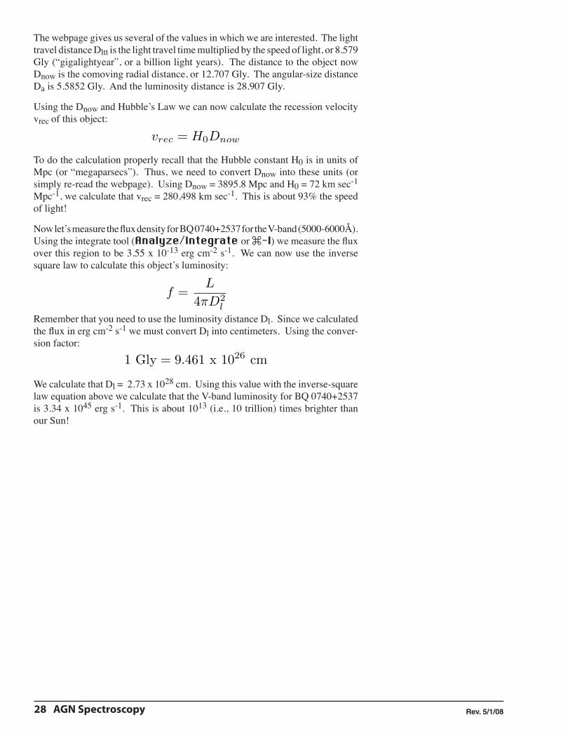
shape of the emission line, such that the peak is not necessarily a good measure of the line’s wavelength. Using the examine tool, the measured wavelengths of the line on the left is roughly 4334.5Å.

Now measure the other broad emission line in the red part of the spectrum. The measured wavelengths of this line is 6377.0Å.

You can now determine their ratio by dividing the longer wavelength by the shorter (so that your ratio is greater than one). For two lines measured above the ratio is 6377.0 / 4334.5 = 1.471. Looking at the table on p. 20, this ratio is close to the ratio of 1.47, which suggests that these are the MgII and C III] emission lines. Since CIII] has an intrinsic rest wavelength that is shorter than MgII, the line on the left must be CIII] and the line on the right must be MgII.

Determining a Redshift

We can now determine a tentative redshift for both lines by using the formula:

1 + z =λobs

λrest

As defined before z is the redshift, λobs is the observed wavelength of a line and λrest is the “rest” wavelength (i.e., if the object was not moving). For the emission line tentatively identified as MgII, which has a rest wavelength of λrest = 2798Å, the calculated redshift is z = 1.27912. For C III], which has a rest wavelength of λrest = 1909Å, the redshift is z = 1.27056. Although not exactly identical these

AGN Spectroscopy 27

redshifts are close to each other. If these were not close (within approximately 0.01) we would suspect that either the line ratio we chose is wrong or that we made in error in calculating the redshift. The average of the two is z = 1.275, which we will adopt as the redshift.

Finding these two relatively strong emission lines (for this object, at least) is solid evidence that this is the correct redshift; however it is not always clear, especially if we don’t know if one or both of the lines are real. Thus it helps to confirm a tentative redshift by identifying additional lines in the spectrum. One approach is to look for other strong emission lines at your tentative redshift. For example, in this object, the CIV line is a good line to look for because is a strong emission line often found in AGN spectra whose wavelength is bluer, but relatively close to CIII]. If the tentative redshift of z = 1.275 is correct, we would find it at 3523Å [1549Å x (1+1.275) = 3523Å]. This is too far in the blue and off the left side of our plot. Similarly, the Hβ emission line would be too far off of the right side of the plot. Another approach is to look for other possible emission lines in the spectrum and see if their positions match known emission lines. Unfortunately no other possible lines are seen in this example. But since we detect two strong emission lines that are clearly real (and have the right ratio for the two strong lines CIII] and MgII) we conclude that this redshift is well established.

Determining Distances, Velocity and Luminosity

Now we can determine this object’s distances via Ned Wright’s cosmology cal-culator. Use the values z = 1.275, H0 = 72, Wm = 0.27, and Wvac = 0.73, and then click on the “general” button. The following results should appear:


The webpage gives us several of the values in which we are interested. The light travel distance Dltt is the light travel time multiplied by the speed of light, or 8.579 Gly (“gigalightyear”, or a billion light years). The distance to the object now Dnow is the comoving radial distance, or 12.707 Gly. The angular-size distance Da is 5.5852 Gly. And the luminosity distance is 28.907 Gly.

Using the Dnow and Hubble’s Law we can now calculate the recession velocity vrec of this object:

vrec = H0Dnow

To do the calculation properly recall that the Hubble constant H0 is in units of Mpc (or “megaparsecs”). Thus, we need to convert Dnow into these units (or simply re-read the webpage). Using Dnow = 3895.8 Mpc and H0 = 72 km sec-1 Mpc-1, we calculate that vrec = 280,498 km sec-1. This is about 93% the speed of light!

Now let’s measure the flux density for BQ 0740+2537 for the V-band (5000-6000Å). Using the integrate tool (Analyze/Integrate or ü-I) we measure the flux over this region to be 3.55 x 10-13 erg cm-2 s-1. We can now use the inverse square law to calculate this object’s luminosity:

f =L

4πD2

l

Remember that you need to use the luminosity distance Dl. Since we calculated the flux in erg cm-2 s-1 we must convert Dl into centimeters. Using the conver-sion factor:

1 Gly = 9.461 x 1026 cm

We calculate that Dl = 2.73 x 1028 cm. Using this value with the inverse-square law equation above we calculate that the V-band luminosity for BQ 0740+2537 is 3.34 x 1045 erg s-1. This is about 1013 (i.e., 10 trillion) times brighter than our Sun!

AGN Spectroscopy 29

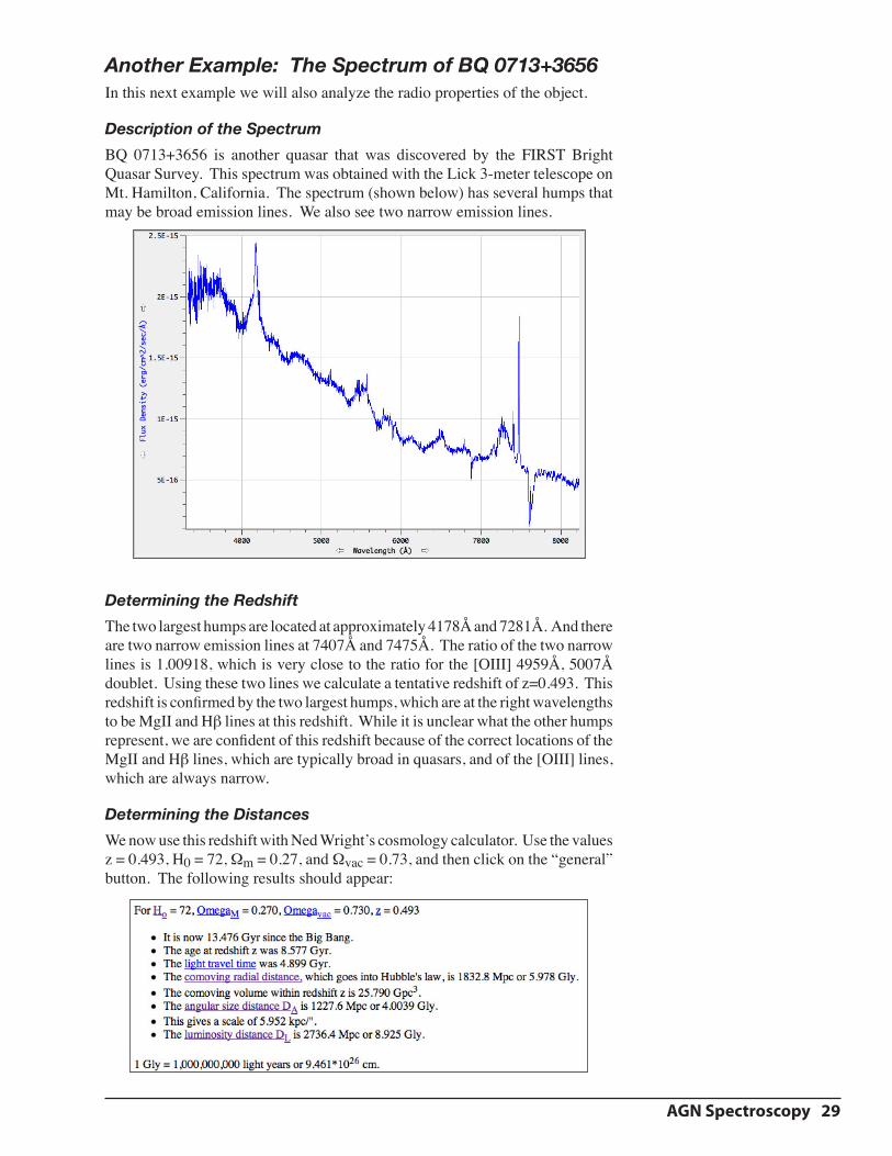
Another Example: The Spectrum of BQ 0713+3656In this next example we will also analyze the radio properties of the object.

Description of the Spectrum

BQ 0713+3656 is another quasar that was discovered by the FIRST Bright Quasar Survey. This spectrum was obtained with the Lick 3-meter telescope on Mt. Hamilton, California. The spectrum (shown below) has several humps that may be broad emission lines. We also see two narrow emission lines.

Determining the Redshift

The two largest humps are located at approximately 4178Å and 7281Å. And there are two narrow emission lines at 7407Å and 7475Å. The ratio of the two narrow lines is 1.00918, which is very close to the ratio for the [OIII] 4959Å, 5007Å doublet. Using these two lines we calculate a tentative redshift of z=0.493. This redshift is confirmed by the two largest humps, which are at the right wavelengths to be MgII and Hβ lines at this redshift. While it is unclear what the other humps represent, we are confident of this redshift because of the correct locations of the MgII and Hβ lines, which are typically broad in quasars, and of the [OIII] lines, which are always narrow.

Determining the Distances

We now use this redshift with Ned Wright’s cosmology calculator. Use the values z = 0.493, H0 = 72, Wm = 0.27, and Wvac = 0.73, and then click on the “general” button. The following results should appear:


Determining the Optical Luminosity

Using the integrate tool in GA3 we find that the total V-band flux density from 5000Å to 6000Å is about 1.131 x 10-12 erg cm-2 s-1. Using the luminosity distance Dl and the inverse square law we find that the optical luminosity over this wavelength range is 1.01 x 1045 erg s-1. This is about 1/3 as luminous as the quasar BQ 0740+2537 from the previous example.

Downloading the Radio Image

We are now going to study the radio properties of this quasar. Since this quasar is located in the area of the sky covered by the FIRST VLA survey, we can download VLA radio images of this object with the FIRST cutout server, which is located online at:

http://third.ucllnl.org/cgi-bin/firstcutout

Follow this URL and you’ll be taken to a page that looks as shown below:

To retrieve a cutout we must first find the celestial coordinates (i.e., the RA and Dec) of this quasar. The coordinates for all of the BQ quasars are given in the text file “bq_list.txt.” Scrolling down to our object we find that its coordinates are “07 13 09.447 +36 56 06.60”. Enter this string of numbers exactly as shown (but without the quote marks) into the RA and Dec text box. And set the image type to GIF. Click on the “Extract the Cutout” button and the following should appear:

If image shown above doesn’t appear, check to make sure that you have the coordinates entered correctly. Also make sure that the default settings are set

AGN Spectroscopy 31

as shown above.

This image shows what the object looks like at radio wavelengths. But to analyze the image we will need to download a FITS file. This can be done either by selecting “FITS File” as the image type and clicking the “Extract the Cutout” button again. Or you can simply click on the extracted image itself. Both should cause a file titled ‘J071309+365606.fits’ to be downloaded.

Determining the Radio Flux Density and Luminosity

To analyze the radio image:ì Launch ImageJ.ì Open and rescale the image:

• Use File/Open... (ü-O) and select the file ‘J071309+365606.fits’ • Open the brightness & contrast control panel with Image/Adjust/

Brightness & Contrast. You may want to zoom in to magnify the image. Move the ‘maximum’ slider to the left until the image looks close to as shown below:

Now we wish to determine the radio flux density:ì Draw a box around the source with the ‘Rectangular Selection’ tool.

The box should be no larger than what is necessary to enclose the entire object (as shown below):

ì Measure the object’s flux density:

• Select Analyze/Set Measurements... and make sure that the ‘integrated density’ option is selected (as shown to the right). Also set the decimal places to 3.

• Select Analyze/Measure (ü-M) and a window with the measure-

The measurement options should be set as shown above. In particular, the ‘integrated density’ should be selected. And the decimal places should be set to 3.


Nomenclature:Radio flux density is measured in units of ‘Janskys’ (Jy). The Jansky is defined as:

1 Jy = 10−26 W m−2 Hz−1

Note that this is a monochro-matic flux density, meaning that it is the flux density as measured at a single frequency. in the case of the FIRST survey, it is a frequency of about 1.4 GHz, which corresponds to a wave-length of about 20 centimeters. In comparison, the optical flux density was measured over a range of wavelengths (i.e., from 5000Å to 6000Å). For this reason the optical and radio flux densities cannot be compared directly.

ment results (like shown below) should appear:

From this window we can read that the integrated flux density (IntDen) is 5.648. Note that this number will vary slightly depending on the size and location of your box. The units of flux density are in Janksys (Jy), so the total radio flux density from this object is 5.648 Jy.

To calculate the radio luminosity of this object we use the inverse-square law in much the same way as we did for calculating the optical luminosity. We will still use the luminosity distance (as determined from Ned Wright’s cosmology calculator). However, we must now convert the distance into meters. We calculate that the radio luminosity is about 5.05 x 1027 W Hz-1.

Measuring Angular and Linear Distances

At optical wavelengths quasars look like nothing more than points of light (i.e., just like a star). But at radio wavelengths they often have extended structure, from jets of energized plasma shooting out of the AGN and into space. The material from the jets collects into giant “lobes” outside of the galaxy. In the case of our quasar, we clearly see the AGN itself (usually called the “core”). It is the bright dot at the center of the image. While the jets are not clearly seen, we do clearly see two lobes, on opposite sides of the core. We wish to measure how far from the AGN the energetic plasma is ejected into space. To do this we must first measure the angular distance from the core to each lobe. We then will convert these measurements into linear distances. To measure the pixel lengths:

ì In ImageJ, select the ‘straight line selections’ tool. If the box from the rectangle selection tool is still present, click outside of the box (but inside the image) to get the box to disappear. Click and drag from the core to the outer edge of each lobe. As you drag the cursor (with the mouse button held down), you will see the length of the line shown under the main toolbar. I measure the distance to the left lobe from the core to be about 21.8 pixels, and the distance to the right lobe from the core to be about 22.5 pixels.

The pixel scale for each image from the FIRST survey is 1.8 arcseconds per pixel. So, the angular distances to the left lobe is 39.2”. And the distance to the right lobe is 40.5”. The angular size q of an object depends on its linear size and the distance to the object by the simple relation:

θ =

d

Da

Where ‘d’ is the linear size of the object, and Da is the angular distance to the object, as determined by the cosmology calculator. Note that the angular size must be in units of radians. To use this equation you must therefore convert the angular distances measured with ImageJ from arcseconds into radians. Alternatively, one may notice that the cosmology calculator conveniently also gives a conversion factor, noting that at this redshift 1” corresponds to 5.952 kpc. Thus, the linear sizes of the left and right lobes are 233.6 kpc and 241.1 kpc respectively. For a sense of scale, note that the distance across our Milky Way galaxy is about 30 kpc. That means that each jet of plasma is travelling a distance almost ten times the size of our galaxy!

Diagram of a typical double-lobed radio AGN. (Image by C. Carilli)

Nomenclature:There are two units used when measuring angles: degrees and radians. There are 360° in an entire circle. And there are 2p radians in a circle as well. Thus, one radian equals about 57.3°.

Each degree can be subdivided into smaller units. Specifically 1° = 60 arcmin, and 1 arcmin = 60 arcsec. As shorthand, single quote marks are used for arcminutes, and double quote marks are used for arcseconds. For example, 1° = 3600”.

AGN Spectroscopy 33

Another Example: The Spectrum of S5 0454+844Description of the spectrum

S5 0454+844 is a BL Lac object in the Strong Source #5 catalog of radio sources. In this example we will search for absorption line doublets.

Measuring wavelengths of absorption lines

Open the file ‘s5_0454p844.ga3.’ The spectrum of S5 0454+844 should look as shown below. It is smooth except for several sets of absorption lines. It does not appear to have any emission lines.

Nearly all of the absorption lines are telluric lines, which are due to the Earth’s atmosphere. However, there is a closely-spaced pair of absorption lines at 6542Å and 6559Å (shown below). The ratio of these two lines is 1.0026, indicating that this is the MgII doublet. It is determined to be at a redshift of z = 1.340.

As discussed before, MgII is a very strong galactic absorption line, thus it is not surprising that we do not see any other absorption features (they are probably too weak to detect). Since there are no emission lines in the spectrum it is a BL Lac object. We do not know whether or not the MgII absorption lines belong to the BL Lac’s host galaxy or to another galaxy that is in front of the BL Lac. Thus the measured redshift of z = 1.340 is only a lower limit to the BL Lac’s redshift.


Yet Another Example: The Spectrum of MS 1408+59Description of the spectrum

In this example we will calculate the redshift and the strength of the “calcium break” in the spectrum of MS 1408+59, a BL Lac object discoverd by the Ein-stein X-ray satellite. Its redshift is more typical of BL Lacs. Its spectrum, shown below, was obtained with the Palomar 5-meter telescope.

Measuring wavelengths of absorption lines

Open the file ‘ms1408p59.ga3’ The spectrum of MS 1408+49 does not show any emission lines, however there are several absorption lines:

First, we see an absorption doublet (two closely spaced absorption lines) at 5857Å and 5934Å. The doublet is identified as CaII because its line ratio is 1.0080. For the doublet to be at these wavelengths, the object must be at a redshift of at z = 0.496. We also see the “CaII break,” where the continuum flux drops slightly blueward of the CaII doublet. Looking for other galactic absorption lines at z = 0.496 we find G-band at 6442Å, Mg “b” at 7733Å and Na “D” at 8818Å.

Measuring the calcium break strength

To determine the calcium break strength we use the equation:

Break =Fr − Fb

Fr

Fb is the continuum flux level blueward of the CaII absorption lines, from 3750Å to 3950Å, and Fr is the flux just redward, from 4050Å to 4250Å in the object’s rest frame. In practice you must shift the wavelength ranges you measure to take into account the redshift of the object. In this example the object is at a redshift of z = 0.496, so Fb should be measured from 5610Å to 5909Å and Fr is measured from 6059Å to 6358Å.

ì To measure the calcium break in GA3:

• Using the cursor, select the region of the spectrum from 5610Å to 5950Å.

• Select Statistics from the Analyze menu. A text box should appear.

The HEAO-2 X-ray observatory. After launch it was renamed in honor of Albert Einstein. It was the first X-ray imaging telescope to be put into space. It operated from November 1978 to April 1981.

The Palomar 5-meter (200-inch) telescope is owned and oper-ated by the California Institute of Technology.

AGN Spectroscopy 35

The mean value given is Fb. In this example, Fb = 2.08 x 10-17. • To find Fr, select the region of the spectrum from 6059Å to 6358Å and

select Statistics again from the Analyze menu. In this example, Fr = 2.29 x 10-17.

There should now be two text boxes that give the statistics for each portion of the spectrum (as shown below):

Putting the measured values for Fb and Fr into the calcium break strength equa-tion we find the break strength for this object to be 0.092, or 9.2%.

AGN Spectroscopy 36

AGN SpectroscopyName(s) Class

Date Lab NotebookDo the following for each object you study:

• Search for emission lines in the spectrum. Identify as many lines as you can.

• Determine a redshift for the object from any emission lines you have discovered.

• Determine the FWHM of the emission lines. Do you consider any of these lines to be broad?

• Search for absorption lines in the spectrum and try to determine their redshift(s). Are they at the same redshift as the emission lines?

• If you found the CaII absorption line doublet, estimate the break strength.

• How fast is it moving away from us? What fraction of the speed of light is this?

• Find the distance to the object (in Mpc).

• At this distance how long would it take light from this object to travel to us?

• Measure the flux in one or more of the B, V, R and I bands.

• Calculate the luminosity for each spectral band you measure.

• Compare its luminosity to the elliptical galaxy NGC 3245.

For all of the objects you study:

• Which class, or classes, of object is the most common in the survey?

• Which objects are the closest, and which are the furthest away?

agn spectroscopy - university of alaska systemrbseu.uaa.alaska.edu/projects/agn/agn...

Documents