Agglomeration and regional growth

Richard E. Baldwin and Philippe Martin

Graduate Institute of International Studies (Geneva) ; University of Paris1 Panthéon-Sorbonne, CERAS-ENPC (Paris) and CEPR

* This is the draft of a chapter for the Handbook of Regional and Urban Economics: Cities andGeography edited by Vernon Henderson and Jacques-François Thisse

2

1. Introduction: why should we care about growth and geography?

2. The basic framework of growth and agglomeration

3. The case without localized spillovers: growth matters for geography

3.1. The growth equilibrium

3.1.1. Endogenous growth and the optimal savings/investment relation

3.1.2. The role of capital mobility

3.2. Perfect capital mobility: the location equilibrium

3.2.1. Stability of the location equilibrium

3.2.2 Does capital flow from the rich to the poor?

3.3. No capital mobility: “new growth” and “new geography”

3.3.1. Stability of the symmetric equilibrium

3.3.2 The Core-Periphery equilibrium

3.4. Concluding remarks

4. The case with localized spillovers: geography matters for growth (and vice versa)

4.1. Necessary extensions of the basic model

4.2. The case of perfect knowledge capital mobility

4.2.1 Spatial equity and efficiency

4.2.2 Welfare implications

4.3. The case without capital mobility: the possibility of a growth take-off andagglomeration

4.3.1 The long-run equilibria and their stability

4.3.2 Possibility of catastrophic agglomeration

4.3.3 Geography affects growth

4.3.4 Can the Periphery gain from agglomeration?

4.4. The geography of goods and ideas: stabilising and destabilising integration

4.4.1 Globalisation and the newly industrialised countries

4.4.2 The learning-linked circular causality

5. Other contributions

6. Concluding remarks

3

1. INTRODUCTION

Spatial agglomeration of economic activities on the one hand and economic growth on theother hand are processes difficult to separate. Indeed, the emergence and dominance of spatialconcentration of economic activities is one of the facts that Kuznets associated with moderneconomic growth. This strong positive correlation between growth and geographic agglomerationof economic activities has been documented by economic historians (Hohenberg and Lees, 1985for example), in particular in relation to the industrial revolution in Europe during the nineteenthcentury. In this case, as the growth rate in Europe as a whole sharply increased, agglomerationmaterialized itself in an increase of the urbanization rate but also in the formation of industrialclusters in the core of Europe that have been by and large sustained until now. The role of citiesin economic growth and technological progress has been emphasized by urban economists(Henderson, 1988, Fujita and Thisse, 1996), development economists (Williamson, 1988) as wellas by economists of growth (Lucas, 1988). At the other hand of the spectrum, as emphasized byBaldwin, Martin and Ottaviano (2001), the growth takeoff of Europe took place around the sametime (end of eighteenth century) as the sharp divergence between what is now called the Northand the South: growth sharply accelerated (for the first time in human economic history) at thesame time as a dramatic and sudden process of agglomeration took place at the world level.Hence, as put by Fujita and Thisse (2002b), “agglomeration can be thought as the territorialcounterpart of economic growth.”

Less dramatically and closer to us, Quah’s results (1996) suggest also a positive relationbetween growth and agglomeration. He finds that among the Cohesion group of countries(Greece, Spain, Portugal and Ireland, though there are no Irish regional data), the two countriesthat have achieved a high rate of growth and converged in per capita income terms towards therest of Europe (Spain and Portugal) have also experienced the most marked regional divergence,This is consistent with the results of De la Fuente and Vives (1995), for instance, building on thework of Esteban (1994) who suggest that countries have converged in Europe but that thisprocess of convergence between countries took place at the same time as regions inside countrieseither failed to converge or even diverged. There are however few direct empirical tests of therelation between agglomeration and growth. Ciccone (2002) analyses the effects of employmentdensity on average labour productivity for 5 European countries at the Nuts 3 regional level. Hefinds that an increase in agglomeration has a positive effect on the growth of regions. An indirecttest of the relationship is performed in the literature on localized technology spillovers. Thepresence of localized spillovers has been well documented in the empirical literature. Studies byJacobs (1969) and more recently by Jaffe et al. (1993), Coe and Helpman (1995 and 1997),Ciccone and Hall (1996) provide strong evidence that technology spillovers are neither global norentirely localized. The diffusion of knowledge across regions and countries does exist butdiminishes strongly with physical distance which confirms the role that social interactionsbetween individuals, dependent on spatial proximity, have in such diffusion. A recent study byKeller (2002) shows that even though technology spillovers have become more global with time,“ technology is to a substantial degree local, not global, as the benefits from spillovers aredeclining with distance. » The fact that technology spillovers are localized should in theory leadto a positive link between growth and spatial agglomeration of economic activities as being« close » to innovation clusters has a positive effect on productivity. Hence, these empiricalresults point to the interest of studying growth and the spatial distribution of economic activitiesin an integrated framework. From a theoretical point of view, the interest should also be clear.

4

There is a strong similarity between models of endogenous growth and models of the “neweconomic geography”. They ask questions that are related: one of the objectives of the first fieldis to analyze how new economic activities emerge through technological innovation; the secondfield analyzes how these economic activities choose to locate and why they are so spatiallyconcentrated. Hence, the process of creation of new firms/economic activities and the process oflocation should be thought as joint processes. From a methodological point of view, the twofields are quite close as they both assume (in some versions) similar industrial structures namely,models of monopolistic competition which reflects the role of economies of scale in both fields.

In this chapter, we will attempt to clarify some of the theoretical links between growthand agglomeration. Growth, in the form of innovation, can be at the origin of catastrophic spatialagglomeration in a cumulative process à la Myrdal. One of the surprising features of theKrugman (1991) model, was that the introduction of partial labour mobility in a standard “newtrade model” with trade costs could lead to catastrophic agglomeration. The growth analog to thisresult is that the introduction of endogenous growth in the same type of “new trade model” canlead to the same result. A difference with the labour mobility version is that all the results arederived analytically in the endogenous growth version. Growth also alters the process of locationeven without catastrophe. In particular, and contrary to the fundamentally static models of the“new economic geography”, spatial concentration of economic activities may be consistent with aprocess of delocation of firms towards poor regions.

The relation between growth and agglomeration depends crucially on capital mobility.Without capital mobility between regions, the incentive for capital accumulation and thereforegrowth itself is at the heart of the possibility of spatial agglomeration with catastrophe. In theabsence of capital mobility, some results are in fact familiar to the New Economic Geography(Fujita, Krugman and Venables, 1999): a gradual lowering of transaction costs between twoidentical regions first has no effect on economic geography but at some critical level inducecatastrophic agglomeration. In the model presented in this chapter, in the absence of migration,“catastrophic” agglomeration means that agents in the south have no more private incentive toaccumulate capital and innovate. The circular causality which gives rise to the possibility of aCore-Periphery structure is depicted below and as usual in economic geography models ischaracterized by both production and demand shifting which reinforce each other. The productionshifting takes the form of capital accumulation in one region (and de-accumulation in the other)and the demand shifting takes the form of increased permanent income due to investment in oneregion (and a decrease in permanent income in the other region).

5

Figure 1: Demand-linked circular causality (a.k.a. backward linkages)

Capital mobility eliminates the possibility of catastrophic agglomeration because in thiscase production shifting does not induce demand shifting as profits are repatriated. It is thereforestabilizing in this sense. This is in sharp contrast with labour mobility which we know to bedestabilizing. However, capital mobility also makes the initial distribution of capital between thetwo regions a permanent phenomenon so that both the symmetric and the Core-Peripheryequilibria are always stable.

In a second section of this chapter, we will concentrate on the opposite causality runningfrom spatial concentration to growth. For this, we will introduce localized technology spilloverswhich will imply that the spatial distribution of firms will have an impact on the cost ofinnovation and therefore the growth rate.

This chapter uses modified versions of Baldwin (1999), Baldwin, Martin and Ottaviano(2000) and Martin and Ottaviano (1999). The first two papers analyze models of growth andagglomeration without capital mobility. In contrast to the first paper which uses an exogenousgrowth model, this chapter analyses endogenous growth. In contrast to the second paper, werestrict our attention to the case of global technology spillovers. The last paper presents a modelof growth and agglomeration with perfect capital mobility. Baldwin et al. (2003) also treat somecommon themes in chapters 6 and 7.

2. THE BASIC FRAMEWORK OF GROWTHAND AGGLOMERATION

Many of the most popular economic geography models focus on labour, examples beingKrugman (1991), Krugman and Venables (1995), Ottaviano, Tabuchi and Thisse (2002) and Puga(1999). These are unsuited to the study of growth. The key to all sustained growth is theaccumulation of human capital, physical capital and/or knowledge capital – with theaccumulation of knowledge capital, i.e. technological progress having a privileged position. Wethus need a model in which capital exists and its stock is endogenous.

North accumulates more capital

Northern permanent income increases

Northern market size increases

Northern firm profits and return to capital rises

6

To present the basic elements of this literature, we organise the discussion with the helpof a workhorse model. As Baldwin et al (2003) show, introducing capital into a geography modelis relatively simple. The simplest way is accomplished by the ‘footloose capital’ model (FCmodel) due to Martin and Rogers (1995). The FC model, however, takes the capital stock asgiven. Getting to a growth model requires us to add in a capital-producing sector.

Specifically we denote capital as K and labour of L. The capital-producing sector isreferred to as the sector I (for innovation and investment, see below) and this comes on top of thetwo usual sectors, manufactures M and traditional-goods T. The regions (two of them) aresymmetric in terms of preferences, technology and trade costs. The usual Dixit-Stiglitz M-sector(manufactures) consists of differentiated goods. Another difference is that the fixed cost is interms of K. Each variety requires one unit of capital which can be interpreted as an idea, a newtechnology, a patent, machinery etc.. Production also entails a variable cost (aM units of labourper unit of output). Its cost function, therefore, is π +w aMxi, where π is K's rental rate, w is thewage rate, and xi is total output of a typical firm. Traditional goods, which are assumed to behomogenous, are produced by the T-sector under conditions of perfect competition and constantreturns. By choice of units, one unit of T is made with one unit of L. The structure of the basicgrowth and agglomeration model is in figure 2.

Regional labour stocks are fixed and immobile, so that we eliminate one possible sourceof agglomeration. Each region's K is produced by its I-sector. I is a mnemonic for innovationwhen interpreting K as knowledge capital, for instruction when interpreting K as human capital,and for investment-goods when interpreting K as physical capital. One possible interpretation ofthe difference between the situation of capital mobility and one of capital immobility is that in thefirst case K is physical capital (mobility then means the delocation of plants) or as knowledgecapital that is marketable and tradable through patents. The second case, capital immobility,would be more consistent with the interpretation of human capital. In this case, labour immobilityimplies capital immobility. The I-sector produces one unit of K with aI units of L, so that themarginal cost of the I sector, F, is w aI. Note that this unit of capital in equilibrium is also thefixed cost of the manufacturing sector. As one unit of capital is required to start a new variety, thenumber of varieties and of firms at the world level is simply the capital stock at the world level:

*KKK W += . We note n and n* the number of firms located in north and south respectively. Asone unit of capital is required per firm we also know that: *nnK W += . However, depending onthe assumption we make on capital mobility, the stock of capital produced and owned by oneregion may or may not be equal to the number of firms producing in that region. In the case ofcapital mobility, the capital may be produced in one region but the firm that uses this capital unitmay be operating in another region. Hence, the number of firms located in one region is, in thecase of capital mobility, different from the stock of capital owned by this region.

7

Figure 2: The basic structure of the growth and agglomeration model

To individual I-firms, the innovation cost aI is a parameter, however following Romer(1990) and Grossman and Helpman (1991), a sector-wide learning curve is assumed. That is, themarginal cost of producing new capital declines (i.e., aI falls) as the sector's cumulative outputrises. Many justifications of this intertemporal externality, classic in the endogenous growthliterature, are possible. Romer (1990), for instance, rationalizes it by referring to the non-rivalnature of knowledge. We can summarize these standard assumptions on this literature by thefollowing:

* ; /1 ; ; KKKKawaFaL

K WWII

I

I +====& (1)

where K and K* are the northern and southern cumulative I-sector production levels. Note thatspillovers are global: the North learns as much from an innovation made in the South than in theNorth. Below, we introduce localized technological spillovers. Following Romer (1990) andGrossman and Helpman (1991), depreciation of knowledge capital is ignored1. Finally, theregional K's represent both region-specific capital stocks and region-specific cumulative I-sectorproduction. Because the number of firms, varieties and capital units is equal the growth rate of

the number of varieties, on which we will focus, is therefore: gKK WW =/& .We assume an infinitely-lived representative consumer (in each country) with

preferences:

σσααρ

/111

0

/11M

1

0

*

C ; ; ln−+

=

−−∞

=

−

=== ∫∫

KK

iiMT

t

t dicCCQQdteU(2)

where ρ is the rate of time preference, σ is the constant elasticity of substitution among varieties,

1 See Baldwin et al. (2003) for a similar analysis with depreciation.

L, numeraire, w=1

T sector (traditional)- Walrasian (CRS& Perf. Comp.)- unit labor cost

No trade costs ? pT=pT= w=w*=1

North &and South markets

M-sector (Manufactures)- Dixit-Stiglitz monopolistic competition- increasing returns: fixed cost, 1 unit of K- variable cost = aM units of L

Iceberg trade costs

I-sector (Innovation, Investment…)- perfect competition-intertemporal spillovers (2 cases: global or localized)- variable cost for one unit of K = aI

Trade in capital, 2 cases:-perfect capital mobility- no capital mobility

8

and the other parameters have the usual meaning. Utility optimization implies that a constantfraction α of total northern consumption expenditure E falls on M-varieties with the rest spent onT. Optimisation by agents in the North also yields unitary elastic demand for T and the CESdemand functions for M varieties. The optimal northern consumption path also satisfies the

standard Euler equation with log utility which requires2 ρ−= rEE /& (r is the north's rate ofreturn on investment) and a transversality condition. Southern optimization conditions areisomorphic.

On the supply side, free trade in T equalizes nominal wage rates as long as both regionsproduce some T (i.e. if α is not too large). Taking northern labour as numeraire then w=w*=1.As for the M-sector, units are chosen such that aM =1-1/σ so that producer prices of varieties arealso normalized to 1. With monopolistic competition, equilibrium operating profit is the value ofsales divided by σ. Using the goods market equilibrium and the optimal pricing rules, theoperating profits are given by:

1

1)1(

*; **

,;1

)1()1(

; 1

nn

E

nn

Ew

w

nn

E

nn

Ew

w

sss

sss

BKE

bB

bss

sss

sB

KE

bB

−+−

+−+

≡=

≡≡−+

−+

−+≡= −

φφφ

π

τφσα

φφ

φπ σ

(3)

where sE ≡ E/ Ew is north’s share of world expenditure Ew; sn = n/(n+n*) is the share of firmswhich are located in the north, and 0=φ=1 is the usual transformation of transaction costs suchthat φ measures the “free-ness” (phi-ness of trade), with φ=0 implying zero free-ness and φ=1implying perfect free-ness (zero trade costs). When capital is immobile, this share is the share ofcapital owned by the Northern region: sK. Also, B is a mnemonic for the 'bias' in northern M-sector sales since B measures the extent to which the value of sales of a northern variety exceedsaverage operating profit per variety worldwide (namely, bEw/Kw).

3. THE CASE WITHOUT LOCALIZEDSPILLOVERS: GROWTH MATTERS FOR

GEOGRAPHY

As we shall see, the localisation of the learning spillovers drive growth is a majorconcern. We start with the simple extreme case considered by Grossman and Helpman (1991)where spillovers are perfectly global. This assumption is already embedded in equation (1).

2 See Barro and Sala-I-Martin 1995 for a derivation using the Hamiltonian approach. Intuitively, the marginal cost ofpostponing consumption is ρ plus the rate of decline of marginal utility which, given the log preferences is just,

EE /& . The marginal benefit is r, the rate of return on investment. The optimal consumption path must be such thatthe two are equalized so that agents are indifferent to a small intertemporal reallocation of consumption.

9

3.1. The growth equilibriumSince the location of innovation and production are irrelevant to the innovation process

(knowledge spillovers are global and depend only on past I-sector production), the worldwideequilibrium growth rate can be determined without pinning down the spatial distribution ofindustry (the location equilibrium). The easiest and most intuitive way of solving for growthequilibria is to use Tobin’s q (Baldwin and Forslid 2000). The essence of Tobin's approach is toassert that the equilibrium level of investment is characterized by the equality of the stock marketvalue of a unit of capital – which we denote with the symbol v – and the replacement cost ofcapital, F. Tobin takes the ratio of these, so what micro economists would naturally call theM-sector free-entry condition (namely v=F) becomes Tobin's famous condition q =v/F=1.

Calculating the numerator of Tobin's q (the present value of introducing a new variety)requires a discount rate. In steady state, 0/ =EE& in both regions3, so the Euler equations implythat r=r*=ρ. Moreover, the present value of a new variety also depends upon the rate at whichnew varieties are created. In steady state, the growth rate of the capital stock (or of the number ofvarieties) will be constant and will either be the common g=g* (in the interior case), or north's g(in the core-periphery case). In either case, the steady-state values of investing in new units of Kare:

; *

*

gv

gv

+=

+=

ρπ

ρπ

(4)

It can be checked that the equality, v=F, is equivalent to the arbitrage condition present inendogenous growth models such as Grossman and Helpman (1991). The free entry condition inthe innovation sector ensures that the growth rate of the value v of capital is equal to growth rateof the marginal cost of an innovation, F, which due to intertemporal spillovers is –g. With r =ρ,and using the definition of F we get the regional q's:

( ) ( ) ; *

*

gK

qg

Kq

ww

+=

+=

ρπ

ρπ

(5)

In the case of global spillovers, the common growth rate is easy to find because it doesnot depend on geography. The reason is simply that the cost of innovation and the total size of themarket do not depend on the location of firms. Hence, we can just use the special case of thesymmetric equilibrium where sE = sn = 1/2 to find the growth rate.

3.1.1 Endogenous growth and the optimal savings/investment relationUsing equation (3) in that case and imposing that Tobin's q is 1 in equation (5), we get the

following relation between growth and world expenditure Ew: ρ+= gbE w where b≡α/σ as isstandard in the growth literature. It just says that higher expenditure by increasing profits inducesmore entry in the manufacturing sector, which implies a higher growth rate. The otherequilibrium relation between growth and world expenditure is given by the world labour market

3 To see this, use the world labour market equilibrium: ga)E(aEL ww +−+−= 1)/11(2 σ which says thatworld labour supply can be used either in the manufacturing sector, the traditional sector or the innovation sector. Itimplies that a steady state with constant growth only exists if Ew itself is constant.

10

equilibrium: ( ) ga)E(saEL ww +−+−= 1/112 , which states that labour can be used either in themanufacturing sector (recall the unit labour requirement in this sector is normalized to 1-1/σ), inthe T sector or in the innovation sector ( wK& is the production of the sector per unit of time andF=1/Kw is the labour requirement in the innovation sector). Here the relation is negative as higherexpenditure implies that labour resources are diverted from the innovation sector to themanufacturing and traditional sector.

Combining the two we find that the world level of expenditure is simply given

by: ρ+= LE w 2 . Using these equations, the growth rate of the number of varieties and of theworld capital stock is given by:

σα

ρ ≡−−= bbLbg ;)1(2(6)

This shows that when knowledge spillovers are global in scope, the equilibrium growth dependspositively on the size of the world economy (as measured by the endowment of the primaryfactor) and negatively on the discount rate. Importantly, the equilibrium g does not depend ongeography.

Finally, a simple equilibrium relation exists between sE and sK, the northern share ofexpenditures and the northern share of capital ownership. It can be shown that optimizingconsumers set expenditure at the permanent income hypothesis level in steady state. That is, theyconsume labour income plus ρ times their steady-state wealth, FK= sK, and, FK*= (1- sK) in thenorth and in the south respectively. Hence, E = L+ρ sK, and E* = L+ρ(1-sK). Note that this is

another way to check the level of world expenditure as: ρ+==+ LEEE w 2* . Thus, we get:

)21

)(2

(21

2

−+

+=+

+=≡ K

KwE s

LLsL

EE

sρ

ρρ

ρ

(7)

This relation between sE and sK, can be thought as the optimal savings/expenditure function sinceit is derived from intertemporal utility maximization. The intuition is simply that an increase inthe northern share of capital increases the permanent income in the north and leads therefore toan increase in the northern share of expenditures.

3.1.2 The role of capital mobilityHaving worked out the equilibrium growth rate, and thus implicitly defined the amount of

resources devoted to consumption, we can turn to working out the spatial division of industry,i.e., the location equilibrium. From now on two roads are open:

1) we can let capital owners decide where to locate production. Capital is mobile eventhough capital owners are not, so that profits are repatriated in the region where capital is owned.In this case, sn, the share of firms located in the north and sK, the share of capital owned by thenorth, may be different. sn is then endogenous and determined by an arbitrage condition that saysthat location of firms is in equilibrium when profits are equalized in the two regions. Because ofcapital mobility, the decision to accumulate capital will be identical in both regions so that theinitial share of capital owned by the north, sK, is permanent and entirely determined the initialdistribution of capital ownership between the two regions.

11

2) a second solution is to assume that capital is immobile. Presumably, this would be thecase if we focus on the interpretation of capital being human (coupled with immobile agents). Inthis case, the location of production, sn, is pinned down by capital ownership: sn = sK.

As we shall see in detail below, the capital mobility assumption is pivotal. Why is this? Instandard terminology, allowing capital mobility eliminates demand-linked circular causality(a.k.a. backward linkages); capital moves without its owners, a shift in production leads to noexpenditure shifting because profits are repatriated. When capital is immobile, any shock whichfavours production in one region is satisfied by the creation of new capital in that region. Sincethe income of the new capital is spent locally, the ‘production shifting’ leads to ‘expenditureshifting’. Of course, expenditure shifting fosters further production shifting (via the famous homemarket effect), so without capital mobility, the model features demand-linked circular causality.As is well known, this form of linkage is de-stabilising, so – as we shall see in detail below –capital mobility in a growth model is a stabilizing force (Baldwin 1999).

Because the case of capital mobility is simpler, we start with it.

3.2. Perfect capital mobility: the location equilibriumWith capital mobility, an obvious question arises: where does capital locate? Capital

owned in one region can be located elsewhere. Again, the arbitrage condition, which implies thatprofits across regions need to be equal for firms to be indifferent between the two locations, pinsdown the equilibrium location of firms. Using equation (3), and imposing the equality of profits,we get that there is no more incentive for relocation when the following relation between sn andsE is satisfied:

10 ),21

)(11

(21

≤≤−−+

+= nEn sssφφ

(8)

where the equilibrium sn equals unity or zero when the sn implied by (8) is outside the zero-unityrange. This is an example of the “home market” effect. Since (1+φ)/(1-φ) is greater than one, thisrelationship tells us that a change in market size leads to a more than proportional change in thespatial allocation of industry.

Combining equations (7) and (8), we get the equilibrium relation between the share offirms located in the north, sn, and the share of capital owned by the north, sK:

10 )21

)(11

)(2

(21

≤≤−−+

++= nKn ss

Ls

φφ

ρρ

(9)

Note also that if the initial distribution of capital in the north is such that sK > ½, then more firmswill be located in the north than in the south: sn > ½. An increase in the share of capital in thenorth, sK, induces relocation to the north as it increases expenditure and market size there. Notealso that lower transaction costs (higherφ) will reinforce the home market effect, implying that anunequal distribution of capital ownership will translate in an even more unequal distribution offirms.

3.2.1 Stability of the location equilibriumIt is easy to see that the division of industry described above will not change over time.

With perfect capital mobility, operating profits have to be the same in both regions which also

12

implies that the value of capital has to be the same in both regions. Hence, π =π* and q=q*=1.This, together with the assumption of constant returns to scale, and the assumption of globalspillovers (implying that the cost of innovation is the same in both regions) means that the tworegions will accumulate capital at the same constant rate so that any initial distribution of capitalis stable. Moreover, since neither backward nor forward linkages operating in this model withcapital mobility, no “catastrophic” agglomeration scenario can unfold (see Martin and Ottaviano1999). Hence, the equilibrium described by (9) is always stable. In particular, the symmetricequilibrium where sn = sK = 1/2, is always stable for any level of transaction costs on trade ingoods.

To see this point in more detail, one can analyze the effect of an exogenous increase in sn,by a small amount and check the impact of this perturbation on the ratio of profits in the north toprofits in the south. That is, ask the question whether an increase in geographic concentration inthe north decreases or increases the incentive to relocate in the north. The symmetric equilibriumis stable, if and only if ∂(π/π*)/∂sn is negative. Indeed this is the case for all positive levels oftransaction costs since, evaluated at the equilibrium geography:

( ) ( )( )

0)1(

111*

2

2

<−+

−−=

∂

∂

EEn sss φφπ

π

Evaluated at the equilibrium given by (9), an exogenous increase in the share of firms located inthe north always decreases relative profits there, so that it leads firms to go back to the south. Thelocation equilibrium determined in (9) is always stable. The reason is that when more firms locatein the north, this increases competition there (and decreases it in the south).

3.2.2 Does capital flow from rich to poor?An interesting question that can be analyzed in this framework is: “Do firms relocate

towards the north or towards the south?” In economic geography models without growth,industrial concentration implies that firms are destroyed in the south and relocated in the north.Here, the relocation story is richer because of the constant creation of new firms. To see what isthe direction of relocation we need to look at the difference between the share of capital ownedby the north and the share of firms located in north. The expression is easier taking ratios, so:

( ) )

21

()2(1

)1(2 −

+−−−

=− KnK sL

Lss

ρφρφφ

(10)

In the symmetric equilibrium, where both regions are endowed originally with the same amountof capital there is no relocation of course. If the initial distribution of capital is such that sK >1/2,so that the north is richer than the south, then the direction of the capital flows is ambiguous; itdepends on the sign of L(1-φ)-ρφ. If this expression is positive, then sK > sn so that some of thecapital owned by the north relocates to the south.

The ambiguity of the direction of capital flows stems from the fact that it is governed bytwo opposite effects, namely the market crowding effect (which is a dispersion force that makesthe poor capital region attractive because firms installed there face less competition), and themarket access effect (which is an agglomeration force that makes the rich region attractivebecause of its high level of income and expenditure). The first effect dominates when trade isquite closed (φ is low). Note that when the rate of time preference is high or more generally when

13

the return to capital is high, the capital rich region becomes more attractive because the marketaccess effect is reinforced. There is a threshold level of transaction costs that determines thedirection of capital flows. It is given by:

ρφ

+=

LLCP

(11)

When transaction costs are below this level, relocation takes place towards the south and vice-versa. The reason why we attach CP (for Core-Periphery) to this threshold will become clear laterwhen we analyze the case of capital immobility, as we will see that this threshold value is the onefor which the symmetric equilibrium becomes unstable.

An interesting feature here is that concentration of wealth and of economic activities inthe north (sK and sn>½), is compatible with relocation of firms from north to south (sK <sn) whenφ <φCP. This comes from the introduction of growth and the fact that a larger number of newlycreated firms are created and owned by the north than by the south.

3.3. No capital mobility: "new growth" and "new geography"The previous section described a growth and geography equilibrium where agglomeration

forces were present,4 but where no "catastrophe" could take place since all circular causality hadbeen ruled out. As discussed above, eliminating capital mobility in a growth model is actually de-stabilising since anything that changes the spatial allocation of industry and thus capital willsimultaneously change that spatial allocation of expenditure. And, as is well known, the homemarket effect means that any change in expenditure’s spatial allocation induces a knock-onchange in the location of industry.

More formally, restricting capital mobility (together with the assumptions of labourimmobility) has two implications. First, the number of firms and the number of units of capitalowned in a region are identical: sn = sK . Second, because the arbitrage condition of the previoussection does not hold, profits may be different in the two regions. This in turn implies that,contrary to the previous section, the two regions may not have the same incentive to accumulatecapital so that the initial ownership of capital does not need to be permanent. This means that theanalysis will be quite different from the previous section. We will ask the following questionswhich are the usual ones in the “new economic geography” models. Starting from an equaldistribution of capital, the symmetric equilibrium, we will determine under which circumstancesit remains a stable equilibrium. Then we will look at the Core-Periphery equilibrium and againask when this equilibrium is stable.

3.3.1 Stability of the symmetric equilibriumWe first consider interior steady states where both regions are investing, so q =1 and

q*=1. Using (3) and (5) in (6), q = q*=1 and imposing sn = sK we get:

4 We define agglomeration as the phenomenon where the concentration of economic activity creates forces that fosterthe concentration of economic activity. The home market effect, which did operate in the pervious section, showsagglomeration forces are present since a division where sL=sK>½ would not be an equilibrium. Due to the homemarket effect, such a division would encourage further concentration of economic activity in the north.

14

)21

)(11

(21

−−+

+= EK ssφφ

(12)

which of course is just (8) with sn replaced by sK. In other words, it now determines the locationof capital ownership as well as the location of production. Together with equation (7) whichimplied that production shifting led to expenditure shifting, this defines a second positive relationbetween sE and sK, i.e. expenditure shifting leads to production shifting.

The intuition is that a relative increase in northern demand increases profits in the northand therefore the marginal value of an extra unit of capital. In other words, the numerator ofTobin’s q increases in the north. Hence, this raises the incentive to innovate there and the northindeed increases its share of capital sK. The intuition is therefore very close to the “home marketeffect” except that it influences here the location of capital accumulation. Together with theoptimal saving relation of (7), it is easy to check that the symmetric solution sE = sK = ½ isalways an equilibrium, in particular it is an equilibrium for all levels of transaction costs. Thesymmetric equilibrium is the unique equilibrium for which both regions accumulate capital (q =q* =1). However, the fact that there are two positive equilibrium relations between sE and sK , theshare of expenditures and the share of capital in the north, should warn us that the symmetricequilibrium may not be stable. Indeed, in this model a 'circular causality' specific to the presenceof growth and capital immobility tends to de-stabilize the symmetric equilibrium because of thedemand-linked cycle in which production shifting leads to expenditure shifting and vice versa.The particular variant present here is based on the mechanism first introduced by Baldwin (1999)in a neo-classical growth model.

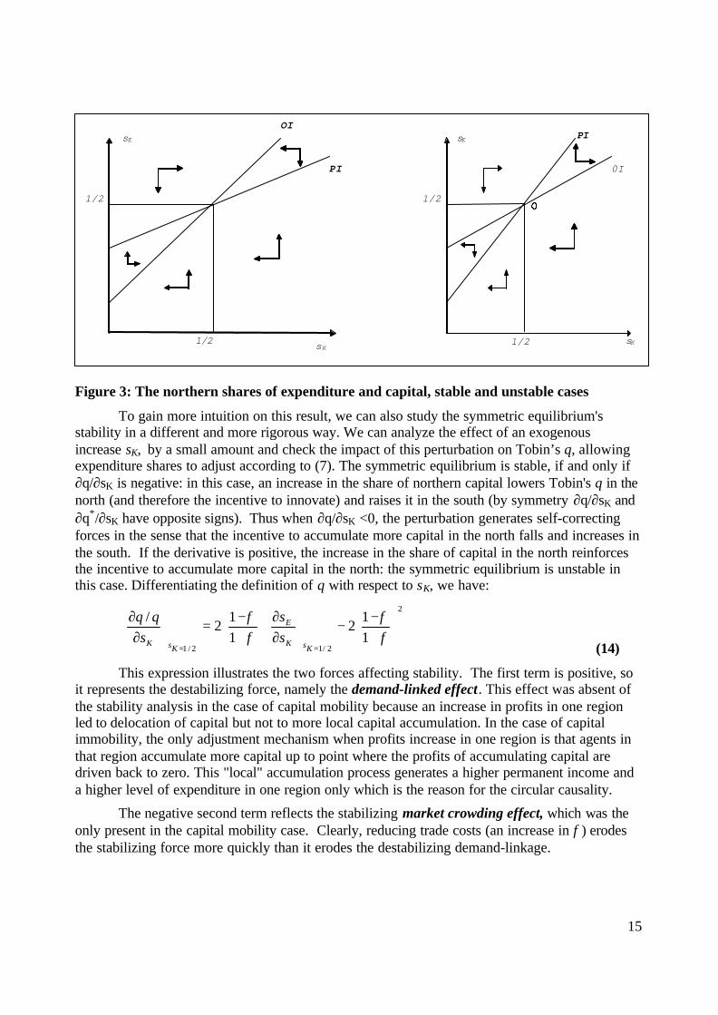
There are several ways to study the symmetric equilibrium's stability. We can first graphthe two equilibrium relations between sE and sK,, the “Permanent Income” relation (call it PI)given by equation (7) and the “Optimal Investment” relation (call it OI) given by equation (12).In the case where the slope of the PI relation is less than the OI relation we get the left-panel ofFigure 3. At the right of the permanent income relation, sE , the share of expenditures in the north,is too low given the high share of capital owned by the north (agents do not consume enough).The opposite is true at the left of the PI relation. At the right of the optimal investment relation, sK

, the share of capital in the north, is too high given the low level of sE , the share of expendituresin the north (agents invest too much). The opposite is true is at the left of the OI relation. Thisgraphical analysis suggests that in this case the symmetric equilibrium is stable.

In the case where the slope of the PI relation is steeper than the OI then the samereasoning leads to the right-panel of the diagram. This suggests that in this case, the symmetricequilibrium is unstable. According to this graphical analysis, the transaction cost below which thesymmetric equilibrium becomes unstable is exactly the one for which the slope of the PI curveequals the slope of OI curve. The slope of the PI curve is: ?/(2L+?) which is the share of capitalincome in total income. The slope of the OI curve is: (1-φ)/(1+φ). The two slopes are equal for alevel of transaction costs which we saw above: it turns out to be the threshold level, which wedefine as φCP, is given by equation (11), namely φCP=L/(L+?). When the "free-ness" of trade ishigher than this level, our graphical analysis suggests that the stable equilibrium is not stable.

15

Figure 3: The northern shares of expenditure and capital, stable and unstable cases

To gain more intuition on this result, we can also study the symmetric equilibrium'sstability in a different and more rigorous way. We can analyze the effect of an exogenousincrease sK, by a small amount and check the impact of this perturbation on Tobin’s q, allowingexpenditure shares to adjust according to (7). The symmetric equilibrium is stable, if and only if∂q/∂sK is negative: in this case, an increase in the share of northern capital lowers Tobin's q in thenorth (and therefore the incentive to innovate) and raises it in the south (by symmetry ∂q/∂sK and∂q*/∂sK have opposite signs). Thus when ∂q/∂sK <0, the perturbation generates self-correctingforces in the sense that the incentive to accumulate more capital in the north falls and increases inthe south. If the derivative is positive, the increase in the share of capital in the north reinforcesthe incentive to accumulate more capital in the north: the symmetric equilibrium is unstable inthis case. Differentiating the definition of q with respect to sK, we have:

2

2/12/111

211

2/

+−

−

∂∂

+−

=

∂

∂

==φφ

φφ

KsK

E

KsK ss

sqq

(14)

This expression illustrates the two forces affecting stability. The first term is positive, soit represents the destabilizing force, namely the demand-linked effect. This effect was absent ofthe stability analysis in the case of capital mobility because an increase in profits in one regionled to delocation of capital but not to more local capital accumulation. In the case of capitalimmobility, the only adjustment mechanism when profits increase in one region is that agents inthat region accumulate more capital up to point where the profits of accumulating capital aredriven back to zero. This "local" accumulation process generates a higher permanent income anda higher level of expenditure in one region only which is the reason for the circular causality.

The negative second term reflects the stabilizing market crowding effect, which was theonly present in the capital mobility case. Clearly, reducing trade costs (an increase in φ) erodesthe stabilizing force more quickly than it erodes the destabilizing demand-linkage.

sE

sK

OI

PI

1/2

1/2

sE

sK

0I

1/2

1/2

PI

16

Using (7) to find ∂sE/∂sK = ρ/[2L+ρ ], the critical level of φ at which the symmetricequilibrium becomes unstable is defined by the point where (13) switches sign. It is easy to checkthat again this critical level is given by φCP of equation (11).

When trade costs are high the symmetric equilibrium is stable and gradually reducingtrade costs produces standard, static effects – more trade, lower prices for imported goods, andhigher welfare. There is, however, no impact on industrial location, so during an initial phase,the global distribution of industry appears unaffected. As trade free-ness moves beyond φCP,however, the equilibrium enters a qualitatively distinct phase. The symmetric distribution ofindustry becomes unstable, and northern and southern industrial structures begin to diverge; to beconcrete, assume industry agglomerates in the north. Since sK cannot jump, crossing φCP triggerstransitional dynamics in which northern industrial output and investment rise and southernindustrial output and investment fall. Moreover, in a very well defined sense, the south wouldappear to be in the midst of a 'vicious' cycle. The demand linkages would have southern firmslowering employment and abstaining from investment, because southern wealth is falling, andsouthern wealth is falling since southern firms are failing to invest. By the same logic, the northwould appear to be in the midst of a 'virtuous' cycle.

3.3.2 The Core-Periphery equilibriumIn addition to the symmetric equilibrium, a core-periphery outcome (sK =0 or 1, but we

will focus only on the second one where the north gets the core) can also exist. For sK =1 to be anequilibrium, it must be that q = v/F = 1 and q* = v*/F* <1 for this distribution of capitalownership: continuous accumulation is profitable in the north since v=F, but v*<F* so nosouthern agent would choose to setup a new firm. Defining the Core-Periphery equilibrium thisway, it implies that it is stable whenever it exists. Using (3), (5) and (6), (7), q* with sK =1simplifies to:

φρρφφ

)2()1(

*22

+++

=L

Lq

(14)

If q* is less than 1 when sK =1, then the Core-Periphery equilibrium exists and is stable asthere is no incentive for the south to innovate in this case. The threshold φ that solves q*=1defines the starting point of the core-periphery set. Again, this threshold is φCP of equation (11).This implies that at the level of the transaction costs for which the symmetric equilibriumbecomes unstable, the Core-Periphery becomes a stable equilibrium.

When transaction costs are high enough, the Core-Periphery equilibrium is not a stableequilibrium: in this case the south would have an incentive to innovate because the profits in thesouth are high enough. This is because even though the southern market is small in this case (ithas no capital income in the Core-Periphery equilibrium), it is protected from northerncompetition thanks to high transaction costs. When transaction costs are low enough, thisprotection diminishes and the fact that the market in the south is small becomes more important:in this case, above the threshold φCP, it becomes non profitable to operate a firm in the south.

Using sK =1, the remaining aspects of the core-periphery steady state are simple tocalculate. In particular, since sK =1, q=1, and q*<1, we have that no labour is used in theinnovation or manufacturing sectors in the south and all innovation is made in the north.

17

Note that the core-periphery outcome (sK =1) is reached only asymptotically. This isbecause the stock of capital in the south does not depreciate and once the level of φCP is crossed,stays constant, whereas the stock of capital in the north keeps growing at rate g. Figure 4summarises the model’s stability properties in a diagram with φ and sK on the axes:

Figure 4: Stability properties of the CP equilibrium

Following the tradition of the “new economic geography” we have analyzed here theexistence and stability conditions of the symmetric and Core-Periphery equilibria. In this simplemodel we can go further and analyze what would happen if we started from a situation in whichthe north had more capital than the south (1/2 <sK <1). It can be checked, using equations (3), (5)and (6) that in this case q <1 (and q*>1) if:

( ) ( ) ( ) 0)1 (1)21

(1 <−−−−− φφρφ Lss KK

that is if φ <φCP. Hence, in this case, the north would not innovate (the large stock of capitalimplies a high degree of market crowding) and the south would innovate. Hence, if we start fromsuch an interior asymmetric equilibrium then one would converge back to the symmetricequilibrium as long as transaction costs are high enough. If φ > φCP, then the economy convergesto the core-periphery equilibrium.

3.4. Concluding remarkComparing perfect capital mobility to no capital mobility, we conclude that:

- when trade costs are high , the absence of capital mobility leads to convergence betweenthe two regions: if one region starts with more capital than the other then, the two regionsconverge to the symmetric equilibrium. On the contrary, with capital mobility, any initialdistribution of capital ownership becomes permanent. However, some of the firms owned by thenorth will relocate and produce in the south. This will produce some sort of convergence interms of GDP but not in terms of GNP.

φ

1/2

φCP

Symmetric (stable)

Symmetric (unstable)

Core-Periphery (stable)

1(free trade)

0(no trade)

1

18

- when trade costs are low, the absence of capital mobility leads to divergence betweenthe two regions5: asymptotically, whatever the initial distribution of capital, all the capital isaccumulated and owned by one region. With capital mobility, as long as all the capital is notentirely owned by the north, some firms will still produce in the south. However, some of thesouthern capital will delocate to the north.

Hence, in the case of mobile capital (physical or tradable innovations such as patents), thekey parameter for regional income distribution is the “exogenous” initial distribution of capital.In the case of immobile (human) capital, the key parameter is the level of transaction costs. Theregional distribution of capital affects the long term regional income distribution “only” to theextent that it determines which region becomes the core, through a small initial advantage incapital endowments for example. To simplify matters we have used a model where only one typeof capital exists. To make it more realistic, in particular for the European case, it would beinteresting to extend it and take into account the different natures of capital so that part of thecapital is mobile and part is not.

Can we derive some policy implications from this analysis? One striking result is thatwhen regions are not well integrated (high transport/trade costs) capital immobility is conduciveto regional convergence6. However, when regions are well integrated, the opposite result is true.To the extent that public policies can alter capital mobility, the policy implication is clear: capitalmobility, both physical and human, should be facilitated between countries which are wellintegrated on the trade side. In the European context, this implies that the "single market" wasright to foster free movement of goods and capital at the same time.

4. THE CASE WITH LOCALIZEDSPILLOVERS: GEOGRAPHY MATTERS FOR

GROWTH (AND VICE VERSA)

In the previous section, we showed that growth could dramatically alter economicgeography in the sense that the process of accumulation of capital teamed with capital immobilitycould lead to catastrophic agglomeration. However, geography had no impact on growth. Thiswas due to the fact that we assumed global spillovers: the learning curve, which as in anyendogenous growth model, was at the origin of sustained growth, was global in the sense that thenorth and the south would learn equally from an innovation made in any region. In this section,we analyze how localized spillovers give a role in growth to the geography of production andinnovation activities.

Localized spillovers are not the only way that geography can affect growth. Martin andOttaviano (2001) generate a feedback between growth and agglomeration by assuming vertical 5 This result however is not general. Urban (2002) integrates a neo-classical growth model into a static geographymodel without physical capital mobility. Contrary to the models presented here, he shows that lower transactioncosts lead to convergence between the poor and the rich country. The reason is that the classic local decreasingreturns effect implies that there is more incentive to accumulate capital in the poor country and in his model thiseffect does not depend on transaction costs. On the contrary, the home market effect, the divergence force, decreasesas transaction costs diminish.6 Basevi and Ottaviano (2002) modify this type of model to investigate the intermediate situation in which capitalmobility is neither absent nor perfectly free.

19

linkages rather than local spillovers in innovation. Because the innovation sector usesmanufacturing goods as an input, the location of manufacturing affects the cost of innovationthrough trade costs. Yamamoto (2002) presents a similar model with circular causation betweengrowth and agglomeration coming from the vertical linkages between the intermediate goodssector and the innovation sector. A different type of geography and growth model where trade isabsent is proposed by Quah (2002). The knowledge spillovers are imperfect both across spaceand time so that quite intuitively spatial clusters can appear. The reasoning is not very differentfrom Grossman and Helpman (1991) who show that when knowledge spillovers are localized theincreasing returns activity concentrates in one location.

4.1. Necessary extensions of the basic modelIntroducing localized technological spillovers requires a minor modification to one of the

assumptions made in the previous section7. Equation (1) that described the innovation sectorassumed global spillovers in the sense that the marginal cost of an innovation, identical in bothregions, was: F= waI =1/KW, so that it was decreasing in the total stock of existing capital; in theGrossman and Helpman (1991), spillovers were global. Grossman and Helpman (1991) alsoconsider the other polar of extreme where knowledge spillovers are purely local. Since the“geography of knowledge” is an important topic for policy makers and a subject that has attracteda great deal of empirical work, it is more convenient to allow non-polar assumptions concerningknowledge spillovers as introduced by Baldwin and Forslid (2000). Specifically, suppose thatthese spillovers are localized in the sense that the cost of R&D in one region also depends on thelocation of firms (stock of knowledge capital). Hence, the northern cost of innovation dependsmore on the number of firms located in the north than in the south so that equation (1) becomes(taking into account that the wage rate is equal to 1):

10, 1 1

≤≤−+≡≡= λλ )s( s A; AK

; aaF nnWII(15)

where λ (a mnemonic for learning spillovers) measures the degree of to which learning fromknowledge creation in one region facilitates knowledge creation in the other region. The fullyglobal spillovers case is where λ=1; the fully local case is λ=0. To put it differently, the higherthe transaction costs on the mobility of ideas, technologies, and innovations. The cost function ofthe innovation sector in the south is isomorphic.

Again the case of perfect capital mobility is easier than the case without capital mobility.Hence, we will start with the former following some of the analysis of Martin and Ottaviano(1999)8 and then describe the model without capital mobility following Baldwin, Martin andOttaviano (2001).

7 Here, localized technology spillovers are assumed. Duranton and Puga (2001) provide micro-foundations for thelink between local diversity and innovation in a model with localized spillovers. Firms that innovate locate indiversified cities and then relocate in specialized cities to commence mass production.8 The set of basic results is enriched by other contributions Ottaviano (1996) as well as Manzocchi and Ottaviano(2001) extend the model of Martin and Ottaviano (1999) to a three-region economy.

20

4.2. The case of perfect knowledge capital mobilityThere are three endogenous variables that we are interested in: the growth rate g which is

common to both regions in steady state; sn, the share of firms that are producing in the north; andsE, the share of expenditure in the north which also can be thought as a measure of incomeinequality between north and south. Remember that with perfect capital mobility, sK the share ofcapital in the north is given by the initial distribution of capital as the stocks of capital in bothregions are growing at the same rate. We want to find the different equilibrium relations betweenthese three endogenous variables.

Due to localized spillovers, it is less costly to innovate in the region with the highestnumber of firms (which represent also capital or innovations). This implies that, because ofperfect capital mobility, all the innovation will take place in the region with a higher number offirms9. Remember that due to perfect competition the value of an innovation is equal to itsmarginal cost. The shares of firms are perfectly tradable across regions (perfect capital mobility)so the value of capital (or firms) cannot differ from one region to another and no innovation willtake place in the south. But the south will be able to simply buy (without transaction costs)innovations or capital produced in the north. Hence, in the case when sK > 1/2, that is when theinitial stock of capital is higher in the north than in the south, we know from the previous sectionthat this will imply that more firms will be located in the north (sn > 1/2) so that all innovationwill take place in the north. In this case the world labour market equilibrium will be given by:

WW

nn

EEss

gL )1(

1)1(

2 ασ

σα

λ−+

−+

−+=

(16)

Remember also that world expenditure is given by: EW= 2L+ρFKW. The value and marginal costof capital is given by F in (15). Using this and equation (16), we get the growth rate of capital gas a function of sn, our first equilibrium relation:

[ ] 12/1 )1()1(2 ≤<−−−+= nnn sbssbLg ρλ (17)

Compared to the growth rate derived in the previous section, this one differs because of thepresence of localized spillovers: spatial concentration of firms (a higher sn) implies a lower costof innovation and therefore a higher growth rate10. Note also that for a given geography ofproduction (a given sn), less localized spillovers (a higher λ) also implies a lower cost ofinnovation in the north (as the innovation sector in the north benefits more from spillovers offirms producing in the south) and a higher growth rate.

The arbitrage condition consistent with the assumption of perfect capital mobility requiresprofits to be equalized in the two locations so that π =π*=bEW/KW. This gives the sameequilibrium relation between sn and sE as in the previous section (equation 8).

9 Fujita and Thisse (2002a and 2002b, chapter 11) show in a version where mobile skilled workers are at the origin ofinnovation, that this sector is always agglomerated in one region. This is the same type of mechanism that applieshere: if capital (in the form of shares, patents etc…) is costlessly tradable and there are localized spillovers that lowerthe cost of innovation in the region with the highest number of innovators, then the symmetric spatial configurationis never stable.10 The result that spatial concentration is good for growth is also present in the model of growth with mobility ofskilled workers by Fujita and Thisse (2002a and 2002b, chapter 11).

21

To find the third equilibrium relation, one between sE and g, remember that due tointertemporal optimization, E= L+ρvK where v is the value of capital which itself is equal to thediscounted value of future profits. Using these relations, it is easy to get the last equilibriumrelation:

)

21

(21

−+

+= KE sg

bsρ

ρ

(18)

Note that income inequality between the two regions is decreasing in the growth rate aslong as the north is initially richer than in the south in capital stocks (sK > ½). This is because thevalue of capital decreases with growth due to faster entry of new firms.

The equilibrium characterized by these three relations is stable for the same reasons as inthe case of perfect capital mobility of the previous section. Capital mobility allows southerners tosave and invest buying capital accumulated in the north (in the form of patents or shares). Hence,the lack of an innovation sector does not prevent the south from accumulating capital: the initialinequality in wealth does not lead to self-sustaining divergence. No “circular causality”mechanism which would lead to a core-periphery pattern, as in the “new geography” models ofthe type of Krugman (1991), will occur.

Using equations (8), (17) and (18), the equilibrium is the solution to a quadratic equationgiven in appendix I. One can find the transaction cost such that relocation goes from north tosouth in the case where sK > 1/2 (which implies also that sn > ½). sK > sn if:

ρλλ

φ++−

+−<

KK

KK

LssLLssL

)1()1(

Note that when all the capital is owned by the north (sK =1), then the threshold level oftransaction cost is again φCP given in the previous section. Note also that in the less extreme casewhere sK <1, less localized spillovers imply, everything else constant, that relocation will takeplace towards the south. The reason is that less localized spillovers imply a lower cost ofinnovation in the north, and therefore a lower value of capital of which the north is betterendowed with. Hence, less localized spillovers generate, for a given distribution of capital, amore equal distribution of incomes and expenditures and therefore attract firms in the south.

One could analyze the properties of this equilibrium by analyzing the equilibrium locationsn given in appendix. However, it is more revealing to use a graphical analysis.

Equation (8) provides a positive relation between sn and sE, the well known “demand-linked” effect. In figure 5, this relation is given by the curve sn (sE) in the NE quadrant. Equation(17) provides a positive relation between g and sn. This is the localized spillovers effect: whenindustrial agglomeration increases in the region where the innovation sector is located, the cost ofinnovation decreases and the growth rate increases. This relation is given by the line g(sn) in theNW quadrant. Finally, equation (19) provides a negative relation between sE and g. This is a“competition” effect: the monopoly profits of existing firms decrease as more firms are created;as the north is more dependent on this capital income, the northern share of income andexpenditures decreases. This relation is described by the curve sE (g) in the SE quadrant.

This graph can be used to analyze the relation between the geography of income, thegeography of production and growth.

22

4.2.1 Spatial equity and efficiencyAn increase in regional inequality in capital endowments sK shifts to the right the sE (g) in

the SE quadrant. The impact is therefore an increase in income inequality and an increase inspatial inequality in the sense that sn increases. However, because the economic geographybecomes less dispersed and therefore more efficient from the point of view of localizedtechnology spillovers, the growth rate g is higher. Hence the introduction of growth and localizedspillovers in a geography model is at the origin of a trade-off between spatial equity andefficiency (see Martin 1999 for an analysis along these lines) which may have importantimplications for public policies.

Figure 5: Spatial equity and efficiency

It is also easy to analyze the impact of lower trade costs on goods (higherφ). For a givenincome disparity, it increases spatial inequality so that the schedule sn(sE) shifts up in the NEquadrant. This in turn increases the growth rate which leads to lower income inequality, an effectthat mitigates the initial impact on spatial inequality. Overall even though spatial inequality hasincreased, the growth rate has increased and nominal income disparities have decreased11.Martin (1999) also shows that lowering transport costs inside the poor region will have exactlythe opposite effect as it leads firms to relocate into that region.

It is also interesting to analyze the effects of an increase in λ that is less localizedtechnology spillovers. This can be interpreted as lowering transaction costs between regions onideas and information. Public policies that improve infrastructure on telecommunication, the

11 These results of course depend on the assumption that agglomeration of economic activities decreases the cost ofinnovation. If congestion costs exist when the agglomeration becomes too large, lowering trade costs betweenregions may have very different effects. Baldwin et al. (2003) show in this case that lower trade costs may lead to anequilibrium with high spatial inequality, high income inequality and low growth.

Equilibrium growth, agglomeration and regional income inequality

sn

sn

g

g

g sE

sE

sE(g)

sn (sE)g(sn)

23

internet or education may be interpreted as affecting λ. This shifts the g(sn ) to the left in the NWquadrant so that growth increases for a given geography of production. This lowers incomedisparities between the two regions as monopolistic profits are eroded by the entry of new firms.This in turn brings a decrease in spatial inequality on the geography of production as sn decreases.More generally, an exogenous increase in growth will lead to less spatial agglomeration and lessregional income inequality. This is important because it implies that, even in the presence oflocalized technology spillovers, the sign of the correlation between growth and agglomerationdepends on the nature of the causal relationship.

4.2.2 Welfare implicationsThe structure of the model is simple enough so that it is fairly easy, at least compared to

the other models, to present some welfare implications. One question we can ask is whether theconcentration of economic activities, generated by market forces, is too small or too importantfrom a welfare point of view (see Baldwin et al. 2003, chapters 10 and 11 for a more detailedanalysis). Two distortions, which are directly linked to economic geography, exist here. First,when investors choose their location they do not take into account the impact of their decision onthe cost of innovation in the north where the innovation sector is located. Localized positivespillovers are not internalized in the location decision and from that point of view the “market”economic geography will display too little spatial concentration. Second the location decisionalso has an impact on the welfare of immobile consumers which is not internalized by investors.This happens for two reasons. On the one hand an increase in spatial concentration affectsnegatively the cost and therefore the value of existing capital so that the wealth of capital ownersin both regions decreases. This affects more the north than the south. On the other hand, whenspatial concentration in the north increases, consumers in the north gain because of the lowertransport costs they incur. Symmetrically, consumers in the south loose. V and V*, the indirectindividual utilities of north and south respectively, as a function of the spatial concentration snand of the growth rate g are given by:

[ ] ( )1

)1(ln)1(

1ln1

2 −+−+

−+

++=

σρα

φσρα

ρg

ssLs? s

CV nnn

K

(19)

[ ] ( )1

s 1ln)1(

)1(1ln

12

*

−++−

−+

−++=

σρα

φσρα

ρg

sLs

s? CV nn

n

K

where C is a constant. We can analyze how a change in the spatial concentration sn affectswelfare in both regions:

)1()1(

nnnKn2

K2

2

n ss-1

1)-( +

ss+sL

s -

1)-(2L

= sV

−+−

∂∂

φφ

σρα

ρσσρλα

(20)

nnnKn2

K2

2

n ss-1

1)-(

ss+sL

s -

1)-(2L

= sV

φφ

σρα

ρσσρλα

+−−

−

−−∂∂

1)1(

1)1(*

There are three welfare effects of a change in spatial concentration. The first term isidentically positive in both regions: an increase in spatial concentration increases growth because,

24

through localized spillovers, it decreases the cost of innovation. The second term is negative inboth regions: the decrease in the cost of innovation also diminishes the value of existing firmsand therefore diminishes the wealth of capital owners. Because the north owns more capital thanthe south, this negative effect is larger in the north than in the south. Finally, the last termrepresents the welfare impact of higher concentration on transaction costs. This welfare effect ispositive in the north and negative in the south.

To analyze whether the market geography displays too much or too little concentration inthe north implies to evaluate these two equations at the market equilibrium. It can be checkedthat as long as λ is sufficiently small (technological spillovers are sufficiently localized), theeffect of an increase in spatial concentration is always positive on the north. It is interesting thatthe north will gain less by an increase in geographical concentration if it owns a larger share ofthe capital. Another way to say this is that capital owners may loose from geographicalconcentration in the north. Geographical concentration in the north may improve welfare in thesouth. This is in stark contrast with standard economic geography models without growth wherethe southerners always loose following an increase in concentration in the north. Here thepositive effect on growth may more than compensate the negative impact of concentration ontransaction costs and on wealth. This will be so if λ is sufficiently small (technological spilloversare sufficiently localized), and if transaction costs are low enough.

4.3. The case without capital mobility: the possibility of a growth take-off andagglomeration

As in the case of globalised spillovers, allowing perfect capital mobility stabilises thelocalised spillovers model by eliminating demand-linked circular causality. We turn now to theopposite assumption – capital immobility. As we shall see, this opens the door to somespectacular interactions between growth and geography.

Here we follow the analysis of Baldwin, Martin and Ottaviano (2001) and simply sketchthe nature of the solution. The model is identical to the one described in the previous sectionexcept for the introduction of localized spillovers as described in the previous section. This hasseveral consequences: the geography of production has now an impact on the cost of innovationso that as in the previous section, the global growth rate is affected by geography. The value ofcapital, which can differ in the two regions as capital mobility is absent, is itself affected bygeography because the innovation sector is perfectly competitive. Hence, the marginal cost ofcapital and innovation is equal to its value. In turn, this affects wealth and expenditures in the tworegions so that profits will depend on geography in this way too. This implies that the tworelations between the share of capital in the north (sK) and the share of expenditures in the north(sE) are going to be much more complex than in the case without localized spillovers.

4.3.1 The long-run equilibria and their stabilityThe optimal savings/expenditure function derived from intertemporal utility

maximisation, which we interpreted as a permanent income relation in the previous section(equation 8) becomes:

[ ]{ }KK

KE sAsALAA

ss

** )1(22)12(

2/1+−+

−+=

ρρλ

(21)

25

where A is given in (15) and A* is the symmetric. The permanent income relation is such that sEis always increasing in sK: an increase in the northern share of capital increases the northern shareof expenditures. When we consider interior steady states where both regions are investing(innovating), so that q =1 and q*=1, the second relation between sE and sK, which we called theoptimal investment one, becomes, in the presence of localized spillovers:

( )[ ]KK

KE sAsA

ss

*2

2

)1(12)2)(12(

2/1+−−−+−

+=φ

φλφλ

(22)

Note of course that sE = sK = ½, the symmetric equilibrium is a solution to the twoequilibrium relations (23) and (24). Two other solutions to this system may exist which are givenby:

1

2 2()-(12

-1 ; 11

11

21

2/1−

−+

≡Λ

Λ−Λ+

−+

±=φλφλ

λφρφλλ

λλ

LsK

(23)

Both sE and sK converge to ½ either as λ approaches 1 or as φ approaches the value:

[ ][ ]ρλλ

ρλρλλρλφ

2)1()1()1()1( 2222

+++++−−++

=L

LLcat

(24)

from above. For levels of φ below φcat, these two solutions are imaginary. In addition, for levelsof φ above another critical value:

)(2)( 4)2(2 22

'

ρλρλρρ

φ+

+−+−+=

LLLLLCP

(25)

one of the solutions is negative and the other one is above unity. Since both violate boundaryconditions for sK, the corresponding steady state outcomes are the corner solutions sK = 0 and sK

=1. Note that for λ = 1, φcat = φCP’= φCP as defined in the previous section.As in the case without localized spillovers, we can study the stability of the Core-

Periphery equilibrium by analyzing the value of q* at sK =1:

[ ])2(

)1( 22

1

*

ρφρφφλ

+++

== L

Lq

Ks (26)

When q* < 1, we know that then the Core-Periphery equilibrium is stable as the south has noincentive to innovate any more. It is easy to check that q*<1, when φ > φCP’.

The stability of the symmetric equilibrium can be studied following the same method asin the case without localized spillovers. We turn to signing ∂q/∂ sK evaluated at the symmetricequilibrium. Differentiating the definition of q with respect to sK, we have:

+−

−−++

++

−

∂

∂2

2

2

2

1)1(

1)1(

11

4φφ

λφφ

λφφ

sdds

+11

2 = s

q/ q

K

E

||K

||

1/2=sK1/2=sK (27)

Using (21) to find [ ]))1()(1(/2/ ρλλλρ +++=∂∂ Lss KE , when evaluated at sK = ½, wesee that the system is unstable (the expression in (27) is positive) for sufficiently low trade costs

26

(i.e. φ ≈1). The two effects discussed in the previous section in the case without localizedspillovers are still present. The first positive term is the demand-linked effect : an increase in sK

increases north’s capital income, expenditure share and local profits so that the value of aninnovation (the numerator of Tobin’s q) increases. The last negative term is the stabilizingmarket crowding effect. The second (positive) term is new and can be thought of as the localizedspillovers effect: an increase in sK implies a lower cost of innovation in the north (thedenominator of Tobin’s q) and therefore increase the incentive to innovate in the north.

4.3.2 Possibility of catastrophic agglomerationIt is possible to show that φcat < φCP’< φCP. Hence, localized spillovers make the

catastrophic agglomeration possible for higher transaction costs. The critical level at which theexpression in (27) becomes positive is φcat. The appendix uses standard stability tests involvingeigenvalues and derives the same result. Figure 6Figure 6 summarises the model’s stabilityproperties in a diagram with φ and sK on the axes. It shows that up to φcat, only the symmetricequilibrium exists and is stable. Between φcat and φCP’, the symmetric steady state looses itsstability to the two neighbouring interior steady states, which are thus saddle points by continuity.This is called a “supercritical pitchfork bifurcation”. After φCP, only the Core-Periphery equilibriaare stable. Note that these can be attained only asymptotically because, due to the absence ofcapital depreciation, the south share of capital never goes to zero even after it stops investing (i.e.after φCP).

Figure 6: Stability properties of equilibria in the presence of localized spillovers

4.3.3 Geography affects growthIntroducing localized technology spillovers implies that economic geography affects the

global growth rate and the model generates endogenous stages of growth. In the version withcapital mobility, the result that geography affects growth was already present. However, because

sK

φ

1/2

φCP’

Symmetric (stable)

Symmetric (unstable)

Core-Periphery (stable)

1(free trade)

0(no trade)

Interior non-symmetric(stable)

φcat

1

27

of the absence of possible catastrophe, the relation between geography and growth was linear.This is not the case here. There are different stages of growth in the sense that if we think thattransaction costs are lowered with time (in line with the “new economic geography” literature),then as economic geography is altered in a non linear way, the growth rate itself changes in a nonlinear manner. When transaction costs are high so that φ < φcat, the equilibrium economicgeography is such that industry is dispersed between the two regions. This implies that spilloversare minimized and the cost of innovation is maximum. Using the optimal investment condition q= q* = 1, and the fact that sK = ½, it is easy to find the growth rate (see also equation (18) usingsK = sn = ½) in that first stage:

)1()1( bbLg −−+= ρλ (28)

The growth rate of course increases with λ. Asymptotically, when sK = 1, spillovers aremaximized so that the cost of innovation is minimized. Again using equation (18) with sK = sn =1, the growth rate is in that stage:

)1(2 bbLg −−= ρ (29)

which is, of course, identical to the solution when spillovers are global since in the core-peripheryoutcome, all innovators are located in the same region and so no learning is diminished by λ.

The growth rate in that final stage is higher than the growth rate in the first stage whentransactions costs are high. In the former stage, innovation has stopped in the south which then isentirely specialized in the traditional good. In the intermediate stage, which we call the take-offstage, i.e. when transaction costs are such that φcat < φ < φCP’, the growth rate cannot beanalytically found. However, it can be characterized as a take-off stage as the pitchforkbifurcation properties of the system entail that the economy leaves a neighbourhood of thesymmetric steady state equilibrium to reach a neighbourhood of the asymmetric steady stateequilibrium in finite time.

We have seen that a gradual lowering of transaction costs on goods (an increase in φ)leads, once the transaction cost passes a certain threshold, to a catastrophic agglomerationcharacterized by a sudden acceleration of innovation in one region (take-off) mirrored by thesudden halt of innovation in the other region. The north (the take-off region) enters a virtuouscircle in which the increase in its share of capital expands its relative market size and reduces itsrelative cost of innovation which in turn induces further innovation and investment. In contrast,the south enters a vicious circle in which lower wealth leads to lower market size and lowerprofits for local firms. It also leads to an increase in the cost of innovation so that the incentive toinnovate diminishes. Hence, growth affects geography which itself affects growth andagglomeration is driven by the appearance of growth poles and sinks.

4.3.4 Can the Periphery Gain from Agglomeration?In most geography models, agglomeration is a win-lose bargain. Residents of the region

that gains the industry typically enjoys an increase in welfare while those left in the periphery seetheir real incomes fall. Allowing for endogenous growth opens the door to an important caveat tothis pessimistic scenario.

28

Growth Compensation for the Periphery

The continual lowering of trade costs produces uneven spatial development – real per-capita income rises in the core region (since it saves the trade costs on all M-varieties) and falls inthe peripheral one (since it pays the trade costs on all M-varieties). However, the emergence ofregional imbalances is accompanied by faster growth in all regions (growth take-off). Of course,this is good also for the periphery and creates a tension between the static loss due to relocationand the dynamic gain due to faster growth. Thus, while the core is unambiguously better off, thetake-off has ambiguous effects of peripheral welfare.

Intuition is served by , which plots the long run levels of welfare in the two regions asfunctions of trade freeness. In particular, it depicts a scenario in which lower trade costs drive allindustry towards the north.

When trade is sufficiently closed, freer trade raises welfare in both regions because itlowers the price of imported manufactured goods. As trade freeness rises above the break point,north and south welfare levels diverge. The north benefits from agglomeration and faster growth.The south benefits only from the latter, while it is harmed by the former. This explains why thesouth’s post-take-off welfare is always below the north’s. Once full agglomeration has beenreached (i.e., freeness has risen above the sustain point), the north’s welfare is constant.

The behaviour of south’s welfare is more complex. If the expenditures share ofmanufacturing goods µ is low enough, the increase in the growth rate has only a mild impact onwelfare and the static loss dominates. In this case, the South loses from the take-off. This case isshown by the solid line (the lowest one in the diagram). On the contrary, if the share µ issufficiently large, the dynamic gain dominates and the take-off benefits both regions, as shownby the dotted line. Finally, for intermediate values of µ, the south initially loses but eventuallyattains a welfare level that exceeds its pre-take-off situation. This is illustrated by the dashedcurve.

Figure 7: Agglomeration, growth and welfare

Welfare

1Free-ness of trade (φ)φΒ φS

north & south

north

South high µ

south medium µ

south low µ

29

Importantly, after the take-off lowering transaction costs always improves welfare in thesouth because it decreases the price of goods imported from the north. Thus, even though thesouth may have been made worse off by agglomeration in the north, resisting further reductionsin transaction costs is not welfare improving.

4.4. The geography of goods and ideas: Stabilising and destabilisingintegration

The main focus in the “new economic geography” literature has been on the consequenceof falling transaction costs on trade in goods. We have shown that in a dynamic model withendogenous growth and localized spillovers, lower transaction costs on goods have an effect onindustry location but also on the growth rate. These effects can be “catastrophic” or not,depending on the mobility of capital.

Economic integration, however, is a multi-faceted phenomenon. Up to this point, we havelook at two types of closer integration – lowering the cost of trade in goods, and making capitalmore mobility. There is another aspect of integration, however, which can also be important,namely integration that results in lower barriers to the spatial diffusion of leaning knowledgespillovers. What might be called the cost of trading ideas. In the model introduced above(localised spillovers and immobile capital) we can study the impact of making trade in ideas freerby changing the ‘learning spillover’ parameter λ12.

12 Keller (2002) shows that technology spillovers have indeed become considerably more global between 1970 and1995.

30

Figure 8:

Falling transaction costs on ideas: Stability properties of equilibria in the presence oflocalized spillovers

4.4.1 Globalisation and the newly industrialised countriesOne exercise that illustrates the interactions focuses on the fact that both φcat and φCP’ are

increasing in λ. The intuition is that as spillovers are becoming more global, an increase in thenorthern share of capital does not decrease much the relative cost of innovation in the north (adestabilizing effect), so that the capital income effect (the stabilizing effect based on lowertransaction costs on goods) must be stronger. One important implication is that from a situationwith full agglomeration in the north (sK = 1) and fixed transaction costs on goods, a gradualincrease in λ (more globalized spillovers due for example to falling telecommunication costs)initially has no impact on southern industry. However, because the cost of innovation in the southdecreases with λ, Tobin’s q in the south increases with λ. At some point, when λ is high enough,q* becomes more than 1, and the south begins to innovate. The value of this threshold levelwhich we call λmir (for “miracle”) is:

2 2

2

1mir ( L ?)

? L( ) ?

φφ φ

+=

+ + (30)

As in the case of falling transaction costs on goods, there is a second critical value wherethe symmetric equilibrium becomes stable. This value, denoted as λmir’ is the level of λ such that∂q/∂sK evaluated at the symmetric equilibrium becomes negative. As with the north take-off, the

sK

λ

1/2

λmir’

Symmetric (unstable)

Symmetric (stable)

1global spillovers

0(no spillovers)

Interior non-symmetric (stable)

λmir

Core-Periphery (stable)

31

“miracle” in the south would appear as a virtuous circle: as it starts investing, its wealth andpermanent income rise so that market size in the south and profits made by local firms increase.In turn, as the number of innovations made in the south increases, the cost of future innovationsdecreases. This “miracle” implies a jump in the investment rate, as Tobin’s q in the south is morethan 1, and rapid industrialization. Also incomes between the south and the north converge. 8describes the effect of an increase in λ on the model’s stability properties in a diagram with λ andsK on the axes.

Figure 9: Stability Map for LS Model: Stabilizing and Destabilizing Integration

4.4.2 The learning-linked circular causalityAnother way to characterise the essential interplay between the cost of trading goods and

ideas is to focus on the symmetric outcome rather than the fully-agglomerated outcome.

It is useful to point out that the localisation of learning in the I-sector creates its owndistinct agglomeration force. This new force, which is very much akin to a cost-linkage thatoperates in the I-sector rather than the I-sector, can be called learning-link circular causality. Thatis, if a region gets a slightly large amount of knowledge, it becomes a more attractive (cheaper)place to produce more knowledge, all else equal. Since a faster rate of knowledge creationsustains and deepens the region’s advantage, an initial bit of ‘knowledge shifting’ leads to‘knowledge-creation shifting’ which in turns leads to knowledge shifting.

Given this logic, it should be clear that making it easier to trade ideas (i.e. raising λ) tendsto stabilise the symmetric equilibrium. We see therefore that there can be a tension between thede-stabilising tendency that arises when goods become cheaper to trade and the stabilisingtendency that arises when ideas become easier to trade.

φ (freeness of trade)

λ (extent of regional knowledge spillovers)

1

1

0

Symmetric stable, CP unstable

Only asymmetric interior equilibra stable

CP stable, symmetric unstable

Integration Path #1:Trade integration only

Integration Path #2:Trade integrationwith pro-spillover policies

Initialpoint

32

To investigate a scenario in which the cost of sharing ideas λ changes together with thecost of trading goods φ, 9depicts what Baldwin and Forslid (2000) call a “stability map”. Thisshows how the model’s stability properties vary with λ and φ. The diagram plots the break andsustain points against the various possible values of λ and φ. The dashed curve is the break pointand the solid curve is the sustain point. The curves partition the map into three regions. Whentrade is not very free, and/or knowledge spillovers are very free, then the symmetric outcome isstable and the CP outcomes are unstable. This is the northwest region in the diagram. When tradeis quite free and/or knowledge flows are very restricted, only the CP outcomes are stable. This isthe southeast region of the map. For a narrow range of φ’s, two asymmetric interior equilibria arethe only stable equilibria and this is shown as the area between the two curves.

The results also point out to a stark difference between lowering transaction costs ongoods and lowering transaction costs on ideas. Lower transaction costs on goods may fosterdivergence in incomes if it triggers an agglomeration process. However, lowering transactioncosts on ideas has the opposite effect as it can make the core-periphery equilibrium unstable andtrigger a sudden industrialization in the south which leads to convergence. In our model, thedistinction between transaction costs on goods and transaction costs on ideas is an easy one.However, in reality trading goods often implies exchanging ideas in the process so that theprocesses that govern the evolution of the two types of transaction costs are certainly intertwined.

5. OTHER CONTRIBUTIONS

An early attempt to link growth and geography models was Walz (1996) who introducesendogenously expanding product variety in a model with vertical linkages and migration. Hisassumption of costless migration leads to a bang-bang migration behaviour. Walz (1997) extendsthe model to a three-region setting.

Black and Henderson (1999) model the relation between urbanization and growth: thereare localized knowledge spillovers so that urbanization affects the endogenous growth of theeconomy. Growth itself affects the size of cities. However, the assumption of a migration processthat is determined by a city developer seems rather restrictive.

The models of growth and geography find their antecedents in models of endogenousgrowth and trade in particular Grossman and Helpman (1991). Some of the results on geographyare already present as these authors show that with free trade and when knowledge spillovers arelocalised, the increasing returns activity concentrates in one location. Models of endogenousgrowth and trade do not however all imply that free trade leads to divergence if trade alsoinvolves capital goods as shown by Goh and Olivier (2002).

Fujita and Thisse (2002a, 2002b chapter 11) propose a combination of a Krugman typecore-periphery model and a Grossman-Helpman growth type model with horizontallydifferentiated products. As in the previous section and the earlier literature on growth andagglomeration, they use a set-up where the fixed cost of firms is a patent. They analyse the twocases of tradability and non tradability of the patents. The skilled workers who produce thesepatents are themselves mobile and they show that this is destabilising factor. In the case oftradable patents, when transaction costs are sufficiently low, a Core-Periphery pattern emergeswith all the R&D sector as well as most of the manufacturing sector concentrated in one region.In this case, agglomeration takes place because of workers mobility and not because of growth

33

but growth is influenced positively by spatial concentration because of the presence of localizedspillovers. With non-tradability of patents, a third destabilising force is added (the first being themobility of skilled workers and the second being the localized spillovers) so that the Core-Periphery becomes sustainable at higher trade costs.

Baldwin (1999) presents a neoclassical growth model combined with an economicgeography model. That paper shows that growth can affect the location industry since changes inregional capital stocks change the relative size of regional markets and this, via the home marketeffect, alters that spatial allocation of industry. The key to this is the fact that forces thatencourage production in one region also tend to encourage capital accumulation in that region. Toput it differently, capital accumulation is another way in which expenditure shifting can be tied toproduction shifting. Moreover, when this demand-linkage is neutralised by assuming that allcapital earnings are repatriated, the linkage is broken.

Figure 10: Real Per Capita Income Changes CP vs CC Models

When capital is immobile, the paper illustrates a second novel feature – geography can affectregional growth, at least in the medium-run. In particular, the Perroux (1955) notion of ‘growthpoles and growth sinks’ appears very clearly. Consider, for instance, initially symmetric regionsfacing trade costs that are high enough to ensure that the symmetric outcome is stable. Whentrade becomes free enough, symmetry becomes unstable. To be concrete, assume a small shockputs the north a little a bit ahead so the core will eventually end up in the north. The instabilityarises since the reward to capital rises in the north and falls in the south. This in turn wouldinduce northern residents to raise their investment rate above the rate necessary to sustain theinitial capital stock. The consequence might be called agglomeration-induced, investment-ledgrowth. The north’s investment rate rises, boosting its capital-labour ratio climbs, and thus its percapita income and output. This expansion of market size further favours investment in the region.In short, the north has become a growth pole. Circular causality has an interesting interpretationin this context. Investment in the growing region is favoured precisely because expenditure in theregion is growing. And expenditure is growing due to the high investment rate.

φ

Per capita real income

1φB

Southern real income CP model

Northern real income, CP model

φ

Per capita real income

1φB

Southern real income CC model

Northern real income, CC model

34

The reverse process operates in the south. The lower rate of return induces southernconsumers/savers to stop investing, so depreciation erodes the southern capital stock and southernper capita income and output begin to drop. Given the particular depreciation process assumed,foreign firms shut down one by one. In the simple models we work with here, workers displacedby the downsizing of the south’s industrial sector immediately find new jobs in the non-industrialsector. However, if finding a new job or expanding the non-industrial sector took time, theperiphery's downward spiral would be associated with above-normal unemployment; the samelabour market features would imply 'labour shortages' in the growing region. More colloquially,the declining region would resemble a 'rust belt' and the ascending region would resemble a'boom belt'.

Allowing growth leads to another feature not commonly found in economic geographymodels that exclude considerations of growth. In the standard Core-Periphery economicgeography model falling trade cost can produce asymmetries in initially symmetric regions. Atintermediate trade costs, the two regions’ also experience divergence of their real per capitaincomes, but eventually, free trade re-equalises incomes. This is illustrated in the left panel offigure 10 with the heavy solid lines (CP model stands for Core-Periphery model) . At the breakpoint, all industry moves north (for convenience, the diagram assumes all H moves immediately)and this raises northern per capita income.

In Baldwin (1999), which assumes capital is immobile, the core-periphery outcomescomes about as a result in a change in the two region’s capital labour ratios, with the north’srising and the south’s falling. Thus even at free trade, the per capita incomes of the north arepermanently higher than those of the south. This is shown in the right panel of figure 10 with CCmodel standing for constructed capital model.

As an aside, we should also note that Baldwin (1999) also added a new element to thegrowth literature, which presumes that such neoclassical growth models predict convergence ofregional income levels. In Baldwin (1999), however, progressive trade liberalisation betweensymmetric nations eventually produces the core-periphery outcome. Thus, contrary to thestandard assertion in the growth literature, in this neoclassical growth model, economicintegration produces divergence in real per-capita income levels.

6. CONCLUDING REMARKS

Introducing growth into economic geography models increases the degree of complexityof models that are already quite complex. Is it worth it? What insights do we gain from themarriage of growth and geography?

Geography and growth models display a number of features that do not appear in moretradition economic geography models such as Krugman (1991). These features are interestingsince they help us organise our thinking about important real-world phenomenon and policies.Specifically:

1. In these models growth affects geography by creating what could be called growth-linkedcircular causality; forces that foster the location of industry in a region also foster the investment,i.e. the accumulation of human, physical and/or knowledge capital in that region. Since these newfactors earn incomes and spend part of these incomes locally, capital accumulation alters relativemarket size.

35

2. The agglomeration process in these models would look like the appearance of growthpoles and sinks – firms want to be in the growing region, people want to invest in that regionsince it is growing and this investment in turn makes the region grow faster. The opposite spiralwould appear to be operating in the ‘growth sink’.

3. The simple geography models predict that everyone should be indifferent toagglomeration once trade became really free. In growth and geography models, region capital-labour ratios ‘endowments’ are permanently altered by agglomeration. Thus regional, real percapital income differentials do not disappear as trade gets perfectly free;

4. Economic integration is a multi-faceted phenomenon in the real world, yet the standardmodels focus almost exclusive in the cost of selling goods at a distance. Economic integration hasa much richer meaning in geography and growth models. Geography and growth models showthat the cost of moving capital across borders (capital mobility) and the cost of moving ideasacross borders (learning spillovers) are also important aspects of economic integration. Inparticular, these other policies can mitigate or extenuate the de-stabilising aspects of freer trade.

5. Perhaps the most important new feature of geography and growth models is the way inwhich they allow us to crystallise our thinking about the interplay between the location ofeconomic activity and the growth rate of economic activity.

6. One aspect of this interplay is important for policy analysis. Taking the standardeconomic geography models at face value produces higher protectionist policy implications (seeBaldwin et al 2003, chapter 12) since agglomeration of industry is always a win-lose situation. Inthe geography and growth models, the result is not so stark. The continual lowering of trade costsdoes produce uneven spatial development – real per-capita income rises in the core region andfalls in the peripheral one. However, the emergence of regional imbalances is accompanied byfaster growth in all regions. Of course, this is good also for the periphery and creates a tensionbetween the static loss due to relocation and the dynamic gain due to faster growth. Thus, whilethe core is unambiguously better off, the take-off has ambiguous effects of peripheral welfare. Asimilar application is to realise that regional policies at the national level that seek to avoidgeography concentration of industry may cost the country as a whole in growth terms. Theintroduction of growth in geography models thus points to the existence of a possible spatialequity-efficiency tradeoff.

7. Perhaps the most sweeping application of these models – and one that is not yet complete– concerns what might be called the grand unified theory of globalisation and geography. Hereare the stylised facts of globalisation since the mid 19th century that the unified theory wouldhave to explain. The world has seen two waves of globalisation – one from roughly 1850 to 1914and one from the 1960s to the present. At a high level of abstraction the key facts are:

Industrialisation/De-industrialisation. In the first wave, the ‘North’ (Western Europe andthe US) industrialised while South (especially India and China) de-industrialised. In the secondwave, the South (East Asia) industrialises while the North de-industrialises.

Divergence. The first wave sees North and South incomes diverge massively, while thesecond wave witnesses a convergence, at least between the North and the industrialising South.

Trade. International trade in goods and factors (labour migration and long-term capitalflows) exploded in the first wave. After being shut down by two world wars, a surge ofprotectionism and the Great Depression, the second wave was marked by a return of trade and

36

capital flows to levels that have recently topped those seen in Victorian England. Massinternational migration, however, remains small by the standards of the first wave.

Growth Take-off. Sometime before the first globalisation wave kicks in, the “IndustrialRevolution” triggers modern growth in the North, but the South continues to stagnant in percapita terms. Modern growth, that is a self-sustain growth process whereby output per hourworked rises steadily year-by-year, begins in the UK but spreads to Western Europe and the USaround the middle of the 19th century. Of course, this it not independent of the incomedivergence since big differences in income levels come from sustained differences in growthrates – not from one-time shifts of the location of industry. Moreover, the limited incomeconvergence in the second wave is linked to spectacular growth in the industrialising South and amoderate slowdown in the North.

Urbanisation. While some of the largest cities in the world were in the South prior to the19th century, the first globalisation wave is accompanied by a rapid and historicallyunprecedented urbanisation in the North. Northern urbanisation continued during the secondwave but cities grew even more rapidly in the South.

The closest the non-growth geography models have come to this is Krugman andVenables (1995), a paper that was known ‘on the streets’ as history-of-the-world-part-I. Thispaper sews together the first three of the five facts as follows. In 1750 or so, the world’seconomic geography was quite homogeneous, i.e. poor and agrarian. With domestic andinternational trade costs nearly prohibitive, each village essentially had to make all its own goods;this meant manufactured goods were dear and the available range of varieties limited. As tradecosts fell, both inside and between nations, specialisation became feasible and this triggered aprocess of what Myrdal called cumulative causality. Modelling this circular-causality process isthe heart of the new economic geography’s contribution, so an aside is in order. Migration offirms or workers de-homogenise the world, turning it into economically big and small regions(markets). When industries are imperfectly competitive and trade is costly, Krugman’s ‘homemarket effect’ favours the location of industry in large regions, but since industries are marked byincreasing returns, getting a disproportionate share of industry means a region’s labour isdisproportionately productive and this in turn results in higher real wages and/or a higher returnto capital. The circle is closed by noting that capital and labour are attracted to the region withhigher rewards and their migration makes the big region bigger and the small region smaller.

According to Krugman-Venables, advances in transport technology in the early 19thcentury triggered this de-homogenisation of the world’s economic geography, and, as historywould have it, the North won at the South’s expense. This single event is the root cause of thefirst three facts: Northern industrialisation and Southern de-industrialisation, the rapid expansionof international trade (England becomes the world’s workshop providing cheap and variedmanufactured goods in exchange for raw materials and this specialisation both fosters trade and isfostered by it), and income divergence (due to increasing returns in industry and decreasingreturns in other sectors, a high share of industry in GDP means high labour productivity and thushigh incomes).

One problem with this story is that the magnitudes just don’t fit. One-time concentrationsof industry just cannot account for the observed income gaps. Here is the argument. Krugman-Venables ignore endogenous technological progress, assuming that physical technology isidentical in the North and South. Thus in the Krugman-Venables story, the difference in incomes

37

between the UK and India must be due to the difference in industry’s share in the UK and Indianoutput mix and the productivity gap between industry and traditional sectors. If the UK’s percapita income was 100 in 1850, India’s was 23 according to Maddison (1995, Tables C16 & D1),so the income gap to be explained is 77. Moreover, Crafts (1989, p.417) tells us that in 1840,47% of the UK workforce was in industry, and Bairoch (1982, Table 9) tells us that India wasonly 4.7% as industrialised as the UK in 1860, so (ignoring the mismatch in dates) we canconclude that the static allocation of industry can only account for the income difference ifindustrial workers are 171 times – i.e. 17,100% – more productive than workers in the traditionalsector.

This just cannot be right. Plainly, the real story must lie elsewhere and growth is theobvious suspect. Indeed, since the headline story in the 19th century was the spread of moderngrowth, the Krugman-Venables story is a bit like Hamlet with the Prince. Clearly, one has to addendogenous growth to the Krugman-Venables story to account for the facts on incomedivergence/convergence as well as on growth take-offs.

As shown in this chapter, allowing for endogenous growth, localised spillovers and somecapital immobility, we can get the fourth fact of globalisation into a unified framework. The onlyfacts left un-accounted for concerns urbanisation. To get this into the story, one would have toallow internal geography in the regions considered, but once the technical difficulties weremastered, the economics would be straightforward. In the first wave of globalisation, economicactivity characterised by localised spillovers is concentrating in the North. It would not thereforebe too surprising that urbanisation proceeded faster in the North than in the South during this era.Likewise, in the second wave of globalisation, the industrialisation of the South (emergence ofthe Asian tigers, etc.) strengthens the forces that foster within South concentration of economicactivity, i.e. urbanisation, while the de-industrialisation of the North does the opposite.

REFERENCES

Baldwin, R. and R. Forslid (1997) Trade liberalization and endogenous growth: A q-theoryapproach, Journal of International Economics 50, 497-517.

Baldwin, R.E. (1999) Agglomeration and endogenous capital, European Economic Review, 43,253-280.

Baldwin, R. and R. Forslid (2000) The Core-Periphery Model and Endogenous Growth:Stabilising and De-Stabilising Integration, Economica 67, 307-324.

Baldwin, R., R. Forslid, P. Martin, G. Ottaviano and Robert-Nicoud, 2003, Economic Geographyand Public Policy, forthcoming, Princeton University Press.

Baldwin, R., P. Martin and G. Ottaviano (2001) Global Income Divergence, Trade andIndustrialization: The Geography of Growth Take-Off, Journal of Economic Growth 6, 5-37.

Barro, R. and X. Sala-I-Martin, 1995, Economic Growth, New York Mc Graw Hill.

Basevi, G. and G. Ottaviano (2002) The district goes global: Export vs FDI, Journal of RegionalScience 42, 107-126.

38

Bottazzi, L. (2001) “Globalization and Local Proximity in Innovation: A Dynamic Process"European Economic Review.

Black, D, and V. Henderson (1999) A theory of urban growth, Journal of Political Economy 107,252-284.

Ciccone, A. (2002) "Agglomeration-Effects in Europe", European Economic Review, Volume46, Issue 2, February , Pages 213-227

Ciccone, A. and R. Hall (1996) Productivity and the Density of Economic Activity, AmericanEconomic Review 87, 54-70

Coe, D. and E. Helpman (1995) International R&D Spillovers, European Economic Review 39,859-887.

Coe, D., E. Helpman and A. Hoffmaister (1997) North-South R&D Spillovers, The EconomicJournal 107,134-149

Duranton G. and D. Puga (2001), "Nursery Cities: Urban Diversity, Process Innovation and theLife Cycle of Products," American Economic Review, vol 5, 1454-1477.

Fujita, M. and J. Thisse, 2002a, “Does Geographical Agglomeration Foster Economic Growth?And Who Gains and Looses from it?” CEPR DP 3135.

----------------------------, 2002b, "Economics of Agglomeration", Oxford University Press.

Grossman, G. and E. Helpman (1991), Innovation and Growth in the World Economy(Cambridge MA: MIT Press).

Goh, A. and J. Olivier, « Learning by doing, trade in capital goods and growth », 2002, Journal ofInternational Economics, 56, 411-444.

Hohenberg P. and L.H. Lees, 1985, The Making of Urban Europe (1000-1950), Cambridge(Mass.), Harvard University Press.

Jacobs, J. (1969) The Economy of Cities (New York: Vintage).

Jaffe A., M. Trajtenberg and R. Henderson (1993) Geographic Localization of KnowledgeSpillovers as Evidenced by Patent Citations, Quarterly Journal of Economics.

Keller W. (2002) Geographic Localization of International Technology Diffusion, AmericanEconomic Review 92, 120-142.

Krugman, Paul (1991) Increasing Returns and Economic Geography, Journal of PoliticalEconomy 99, 483-99.

Krugman P. R. and A. J.Venables (1995) Globalization and the inequality of nations, QuarterlyJournal of Economics 60, 857-880.

Lucas, R.E. (1988) On the mechanics of economic development, Journal of MonetaryEconomics} 22, 3-42.

Manzocchi, S. and G. Ottaviano (2001) Outsiders in economic integration: The case of atransition economy, Economics of Transition 9, 229-249

Martin, P. (1999) "Public Policies, Regional Inequalities and Growth", Journal of PublicEconomics, (73)1 pp. 85-105

39

Martin, P. and G. Ottaviano (1999) Growing Locations: Industry Location in a Model ofEndogenous Growth, European Economic Review 43, 281-302.

Martin, P. and G. Ottaviano (2001) Growth and Agglomeration, International Economic Review42, 947-968.

Martin, P. et C. A. Rogers, 1995, “Industrial Location and Public Infrastructure,” Journal ofInternational Economics, 39, 335-351.

Ottaviano, G.I.P. (1996) The location effects of isolation, Swiss Journal of Statistics andEconomics 132, 427-440.

Ottaviano, G.I.P., T. Tabuchi and J.-F. Thisse (2002) Agglomeration and Trade Revisited,International Economic Review 43, 409-436.Perroux, F. (1995) Note sur la croissance, Economie Appliquée 1-2, 307-320.

Puga D. (1999), The rise and fall of regional inequalities, European Economic Review, vol. 43,pp. 303-334.

Quah, D. (2002), "Spatial Agglomeration Dynamics", CEPR DP 3208.

Romer, P., (1990) Endogenous Technological Change, Journal of Political Economy 98.5, partII, S71-S102.

Urban, D. (2002) "Neoclassical Growth, Manufacturing Agglomeration and Terms of Trade",mimeo LSE.

Waltz, U. (1996) Transport Costs, Intermediate Goods and Localized Growth, Regional Scienceand Urban Economics 26, 671-795.

Walz, U. (1997) Growth and deeper regional integration in a three-country model, Review ofInternational Economics 5, 492-507.

Williamson, J.G., 1988, «Migration and Urbanization », in H. Chenery and T.N. Srinivasan

(eds.), Handbook of Development Economics, volume 1, Amsterdam: North Holland, 425-465.

Yamamoto, K. (2001), Agglomeration and Growth with Innovation in the Intermediate GoodsSector, mimeo, Graduate School of Economics, Kyoto University, forthcoming RegionalScience and Urban Economics.