agency pricing and bargaining: evidence from the e-book market
TRANSCRIPT

Agency Pricing and Bargaining:
Evidence from the E-Book Market∗
Babur De los Santos†
Daniel P. O’Brien‡
Matthijs R. Wildenbeest§
October 2021
Abstract
This paper examines the pricing implications of two types of vertical contracts under bargain-ing: wholesale contracts, where downstream firms set retail prices after negotiating wholesaleprices, and agency contracts, where upstream firms set retail prices after negotiating sales roy-alties. We show that agency contracts can lead to higher or lower retail prices than wholesalecontracts depending on the distribution of bargaining power. We propose a methodology tostructurally estimate a model with either contract form under Nash-in-Nash bargaining. Weapply our model to the e-book industry, which transitioned from wholesale to agency contractsafter the expiration of a ban on agency contracting imposed in the antitrust settlement betweenU.S. Department of Justice and the major publishers. Using a unique dataset of e-book prices,we show that the transition to agency contracting increased Amazon prices substantially but hadlittle effect on Barnes & Noble prices. We find that the assumption of Nash-in-Nash bargainingexplains the data better than an assumption of take-it or leave-it input contracts. Counterfac-tual simulations indicate that reinstitution of most favored nation clauses, which were bannedfor five years in the 2012 settlement, would raise the prices of e-books by seven percent butwould lower profits of the publishers and Amazon.
Keywords: e-books, agency agreements, vertical restraints, bargaining, most favored nationclause
JEL Classification: C14, D83, L13
∗We thank Takanori Adachi, Hanna Halaburda, Julie Holland Mortimer, Ginger Jin, Justin Johnson, HuaxiaRui, Fiona Scott Morton, and Shen Zhang for their useful comments and suggestions. This paper has benefittedfrom presentations at Boston College, Einaudi Institute for Economics and Finance, European Commission (DGCOMP), MIT, Ohio State University, Stanford University, Universite Paris Sud, University of Cologne, University ofMannheim, University of Vienna, Wake Forest University, ASSA Annual Meeting, Berlin IO Day at Humboldt Uni-versity, CEPR Conference on Applied Industrial Organisation, CES North America Conference, EARIE Conference,European University Institute PriTech Workshop, HAL White Antitrust Conference, IIOC Annual Meeting, (IO)2,NBER Summer Institute, and NET Institute Conference. We gratefully acknowledge financial support by the NETInstitute, http://www.NETinst.org. De los Santos is a senior economist at Amazon. The views expressed are thoseof the authors and do not necessarily reflect those of Amazon, Inc. The paper represents work of De los Santos priorto joining Amazon and uses publicly gathered information only.†John E. Walker Department of Economics, Clemson University, E-mail: [email protected].‡Compass Lexecon and Microfoundations, Inc., E-mail: [email protected].§Kelley School of Business, Indiana University and CEPR, E-mail: [email protected].

1 Introduction
In many retail markets, the distribution arrangement involves suppliers charging retailers wholesale
prices and retailers setting final prices to consumers (the “wholesale” model). The wholesale model
has been extensively-studied in the literature and forms the foundation for much of the economics
of vertical contracting, particularly that which informs antitrust policy.1 Another distribution
arrangement that has received much less attention involves agency relationships where suppliers
pay retailers sales royalties to distribute products at prices determined by suppliers (the “agency”
model).2 Agency arrangements are used in some conventional markets (e.g., newspapers sold at
kiosks, insurance sold by independent agents), but they are especially prevalent in online markets.3
Agency arrangements raise interesting questions for both price theory and policy. Key questions
include how the choice of pricing institution affects prices and profits. In a recent antitrust case,
the Department of Justice (DOJ) alleged that Apple and major book publishers engineered a shift
from wholesale to agency pricing in the market for e-books, and that this shift, in combination with
retail price most-favored nation (“MFN”) clauses, raised the prices of e-books. Empirical evidence
(De los Santos and Wildenbeest, 2017) confirms the price increase. A natural question is whether
the price increase was caused by the shift to the agency model, the MFN clause, or both.
Recent theoretical literature has begun to address this question, but the literature to date
has a significant gap: it abstracts from bargaining, which is an important feature of many in-
termediate markets, including the e-book market. Johnson (2017) compares the wholesale and
agency models under the assumption that input terms are established through take-it or leave-it
offers by the entity that is not responsible for setting the downstream price.4 Under a reasonably
weak condition on demand, he finds that the agency model generates lower retail prices than the
wholesale model. But suppose that instead of having the non price-setting firm making take-it
or leave-it offers, the downstream buyer makes the offers instead. In the wholesale model, the
buyer would set the wholesale price equal to upstream marginal cost and thereby eliminate dou-
ble marginalization. In the agency model, by contrast, the buyer would set the royalty looking
ahead to the impact on the upstream firm’s pricing decision, and this would generally lead to a
degree of double marginalization.5 Thus, the comparison between wholesale and agency arrange-
ments is sensitive to the distribution of bargaining power. Yet, the theoretical literature on agency
1For example, the wholesale model forms the basis for most of the discussion of antitrust treatment of verticalintegration and restraints in leading industrial organization textbooks (e.g., Carlton and Perloff, 2004). Note thatwholesale pricing is also commonly referred to as linear pricing.
2Johnson (2017) distinguishes two other pricing arrangements: the “franchise” model, where the suppliers collectsales royalties from retailers that set the retailer price, and the “consignment” model, where suppliers charge awholesale price and also control retail prices. Our focus in this paper is on the wholesale and agency models.
3For example, third-party sellers on Amazon Marketplace (the “upstream” firms) set the retail price for theirproducts, while Amazon (the “downstream” firm) receives a percentage of the revenue. Other examples include eBayBuy It Now and the Apple App Store.
4If the entity with all bargaining power also controls retail prices then it can achieve the vertical integratedoutcome. Hence, take-it or leave-it offers in this context are assumed to be made by the entity without control ofretail prices.
5A form of double marginalization arises in the agency model unless the upstream firm has zero marginal cost.
2

pricing (Gans, 2012; Gaudin and White, 2014; Abhishek, Jerath, and Zhang, 2015; Foros, Kind,
and Shaffer, 2017; Johnson, 2017; Condorelli, Galeotti, and Skreta, 2018; Johnson, 2020) abstracts
from bargaining. The literature on the wholesale model, in contrast, has focused extensively on
bargaining and considers it to be a fundamental economic factor determining outcomes in many
situations.6
In this paper we examine the relationship between agency contracts and retail prices when
intermediate pricing terms are determined through bargaining, and we propose and estimate a
structural model that allows examining both arrangements empirically. We begin in Section 2 by
extending the bilateral monopoly models of wholesale and agency pricing in Johnson (2017) to
allow for bargaining between the supplier and retailer. We show that agency contracts can lead
to higher or lower retail prices depending upon the relative bargaining powers of the upstream
and downstream firms. When the upstream firm has high bargaining power, the wholesale price is
relatively high in the wholesale model but the royalty paid to the retailer is relatively low in the
agency model. In the wholesale model, retailers pass the high input price on to consumers in the
form of higher retail price. In the agency model, by contrast, low royalties give the supplier a larger
share of the retail price and reduce double marginalization, leading to a lower price than in the
wholesale case. The opposite is true when the downstream firm has high bargaining power. In this
case, a low wholesale price in the wholesale model reduces double marginalization and leads to a low
retail price, while a high royalty paid to the retailer in the agency model causes significant double
marginalization and a high retail price. In summary, the retail price tends to be lower in either
arrangement when the firm with high bargaining power also determines the retail price, as the
price-setting firm has an incentive to establish input terms that mitigate double marginalization.
This relationship between bargaining power and retail prices in the wholesale and agency models
plays an important role in the identification strategy in our structural model, as we explain in more
detail below.
In Section 3 we adapt the theoretical model to make it more amendable to estimation by
allowing for multi-product firms and multiple suppliers and retailers, using a logit demand structure.
Following recent literature, we use the “Nash-in-Nash” solution to model bargaining.7 In this
framework each pair of firms reaches an asymmetric Nash bargaining solution while taking the
terms negotiated by other pairs as given. We extend this literature, which has focused on wholesale
6Examples include Horn and Wolinsky (1988) [mergers]; Dobson and Waterson (1997) [countervailing power],O’Brien and Shaffer (2005) [mergers], O’Brien (2014) [price discrimination], Crawford, Lee, Whinston, and Yurukoglu(2018) [vertical integration], and Ho and Lee (2019) [hospital and health insurance pricing].
7The “Nash-in-Nash” solution concept was first applied in the wholesale model by Horn and Wolinsky (1988)to study mergers and by Davidson (1988) to study multi-unit bargaining in labor markets (neither set of authorsused the term “Nash-in-Nash,” which appears to have arisen in the folklore). O’Brien (1989; 2014) provides non-cooperative foundations for this solution concept based on an extension of Rubinstein’s (1982) bargaining modelto environments with upstream monopoly, downstream oligopoly, and linear input pricing. The extension to thecase of multiple upstream firms is straightforward. Collard-Wexler, Gowrisankaran, and Lee (2019) provide a non-cooperative foundation for the Nash-in-Nash solution concept for bargaining that is over fixed transfers that do notaffect downstream firms’ pricing decisions. Our model is different because we allow wholesale prices and sales royaltiesto affect downstream pricing decisions.
3

pricing contracts, to allow for agency contracts between upstream and downstream firms. Moreover,
when deriving the bargaining equilibrium for both types of vertical contracts, we let firms take into
account retail price reactions to input prices.
We apply our model to the e-book industry. This industry is uniquely suited to study the
effects of bargaining under wholesale and agency contracts because the industry has experienced
various transitions between these vertical contracts since the introduction of the Kindle e-reader
in 2007. In Section 4 we describe the changes in contracts between publishers and book retailers
in the e-book industry and how these changes affected retail prices. E-books, similar to printed
books, were initially sold using the wholesale model. In this period, Amazon pursued a low price
strategy for e-books (e.g. $9.99 for newly released e-books). As De los Santos and Wildenbeest
(2017) document, publishers were against this pricing arrangement because they believed that it
cannibalized profitable hardcover sales, eroded consumer perceptions of the value of a book, and
would eventually lead to lower wholesale prices.
With the introduction of the iPad in 2010, major publishers negotiated agency contracts with
Apple to offer e-books for sale in Apple’s new iBookstore. The terms of the agency contracts with
Apple, particularly the MFN clause that required publishers to match lower retail prices at other
retailers, prompted five of the six major publishers (the “Big Six”) to compel the adoption of agency
contracts on Amazon. The industry adoption of agency contracts and the MFN led to higher prices
for e-books. In 2012 the Department of Justice sued Apple and five of the Big Six publishers for
conspiring to raise e-book prices. All five publishers that were sued settled the lawsuit and agreed
to a two-year ban on publisher-set prices, which effectively meant a return to traditional wholesale
contracts. De los Santos and Wildenbeest (2017) analyze the transition from agency to wholesale
contracts following the ban and find that retail prices decreased by 18 percent at Amazon and 8
percent at Barnes & Noble as a result.
The expiration of the two-year ban on agency pricing meant that, by the end of 2014, publishers
could again negotiate agency contracts with Amazon and most other retailers that would allow
them to control retail prices directly—because Apple had not settled, it was subject to a separate
court injunction that banned the use of agency contracts for a longer period. Bargaining between
publishers and retailers played an important role in the renegotiation of existing contracts. In
Section 4 we describe some aspects of the bargaining dispute between Amazon and Hachette,
which included inventory reductions and price increases for Hachette titles. These negotiations
took over six months, were extensively covered by the media, and they involved public pressure by
some of Hachette’s bestselling authors. Despite the lengthy bargaining period, by the end of 2015,
all of the major publishers had returned to agency contracts with Amazon with publisher-set prices.
In Section 4 we also investigate the effect on retail prices following this latest shift towards agency
contracts, using price data for e-books sold at Amazon and Barnes & Noble in the period 2014-
2015. We exploit the variation in the timing of the implementation of the new agency contracts
to estimate the change in retail prices resulting from the switch to the new agency arrangements
4

using a difference-in-differences approach. Our findings indicate that, on average, Amazon prices
increased 14 percent and Barnes & Noble prices decreased 2 percent. The estimates also show
substantial heterogeneity in price effects across publishers. These findings are difficult to explain
using take-it or leave-it contracting models, but they are consistent with a bargaining model in
which publishers have different bargaining weights.8
In Section 5 we discuss how to structurally estimate the empirical model developed in Section 3
in light of the industry transitions discussed in Section 4, and we present estimates of the bargaining
model by jointly estimating demand and supply. The extent to which prices change following a shift
to agency contracts is related to the relative bargaining power of the firms involved. To fully exploit
this mechanism for identification and estimation, we use data from both before and after the latest
switch to agency pricing. Our goal is to obtain estimates of the demand side parameters as well as
supply side parameters, which includes a bargaining parameter for each publisher-retailer pair. Al-
though the supply model varies between wholesale and agency contracts, we assume the bargaining
parameters do not change when switching. This assumption abstracts away from the initial stage
of bargaining between publishers and retailers over the type of contracts (wholesale versus agency)
in order to make the model tractable. Then, for a given set of demand and supply parameters, we
can use the pricing and bargaining first-order conditions for each model to solve for the margins
of the upstream and downstream firms in both periods. We use the margins to back-out upstream
marginal costs, which, assuming a log-linear relation between marginal cost and observable cost
shifters, allows us to obtain estimates of both demand and supply side unobservables.
We use a covariance restriction approach to deal with price endogeneity in the demand equation.
MacKay and Miller (2021) show there is link between the demand and supply side unobservables
and the endogenous price coefficient, and that instrument-free identification of the price coefficient
can be achieved by using a covariance restriction on the unobserved shocks. MacKay and Miller
develop a three-stage estimator for the price coefficient in the simple logit model that is computa-
tionally trivial, assuming constant marginal cost and Bertrand competition. Since the bargaining
parameters enter our supply side model nonlinearly, we use a GMM estimator that exploits cross-
covariance restrictions to create additional moments that are necessary to estimate the additional
nonlinear parameters, following the approach put forward by MacKay and Miller (2021) for the
case of nonlinear parameters. We assume zero cross-covariance between the unobserved demand
and cost shocks and use Monte Carlo experiments to show that this approach effectively deals
with price endogeneity in small samples, while also allowing us to recover the nonlinear bargaining
parameters of the supply side model.
According to our estimates, the price coefficient for the logit specification implies a median own-
8An important difference between the reduced form analysis in this paper and that in De los Santos and Wilden-beest (2017) is that we study transitions between the wholesale and agency model in the absence of an allegedconspiracy, whereas De los Santos and Wildenbeest analyze transitions that resulted from an alleged conspiracyinvolving Apple and competing publishers. In addition, retail price MFN clauses were not used during the periodwe study, allowing us to isolate the effect of agency pricing from the effect of the MFN. This is important, as thetheoretical results of Johnson (2017) indicate that the MFN would have had a positive effect on prices.
5

price elasticity of around −1.8 for our main specification. The supply-side estimates suggest that the
retailers have more bargaining power than the publishers. However, there are substantial differences
in bargaining parameters between different retailer-publisher pairs, and Amazon generally has more
bargaining power than Barnes & Noble. The estimates imply an agency royalty of 39 percent on
average, which is higher than the thirty percent royalty that was common during the first agency
period. It is important to note that these results rely on several simplifying assumptions regarding
the bargaining process—to check for robustness with respect to the agency royalty, we have also
estimated a specification in which the royalty is fixed to 30 percent and find less bargaining power
for Amazon. Moreover, supply side estimates that are obtained using alternative values of the price
coefficient show that we get similar bargaining parameter estimates for a range of price coefficients,
suggesting our bargaining estimates do not rely critically on the covariance restrictions required
by the MacKay and Miller (2021) approach. We compare the fit of the bargaining model to an
alternative model with take-it or leave-it offers by the party that does not control retail prices.
That is, we estimate a model in which retailers make take-it or leave-it royalty offers to publishers
in the agency arrangement, and publishers make take-it or leave-it wholesale price offers to retailers
in the wholesale arrangement. We find that the bargaining model gives a better fit to the data
than the take-it or leave-it specification.
In Section 5 we also discuss the results of a counterfactual analysis where we use the estimates
of the bargaining model to simulate the effect of retail price MFN clauses on retail prices. MFN
clauses in this context are price-parity restrictions that guarantee that the same title is sold at
the same price everywhere, as in the contracts used during the first agency period in the e-book
industry. Price-parity clauses have been used by other online platforms in which agency contracts
are used, such as online travel agencies, and even though U.S. courts have mostly upheld MFN
clauses (Dennis, 1995), they have been under scrutiny by competition authorities around the world
for their potential to reduce price competition.
The settlements between the DOJ and publishers banned the use of MFN clauses for a period
of five years, as they were considered to have played a crucial role in the alleged conspiracy. The
role of MFN has been explored theoretically by Johnson (2017), who finds that it tends to raise
retail prices. In line with this theoretical finding, our counterfactual simulations indicate that prices
would increase an additional seven percent, on average, if retail price MFN clauses were added to
the agency contracts. This finding is consistent with recent work by Mantovani, Piga, and Reggiani
(2021), who analyze the price effects of laws in several European countries that banned the use of
price-parity clauses by online travel agencies and find a significant price reductions in the medium
run, especially for hotels affiliated with a chain. Our simulations also show that reinstatement
of MFN clauses would lower profits of Amazon and the publishers, which could be a factor that
explains why, as far as we know, MFN has not been adopted, despite the ban being lifted. We also
compare the counterfactual predictions to the estimated price difference when using a difference-in-
differences (DID) approach to compare prices during the first agency period (2010-2012) to prices
6

during the current agency period. Although the DID estimates indicate prices were indeed higher
during the first agency period, it is difficult to separate the price effects of MFN clauses from
the price effects of the alleged collusion between the publishers in the first agency period. The
counterfactual predictions based on the estimates of our structural model are obtained assuming
no collusion, and therefore provide more direct estimates of the effect of MFN on agency prices
than is possible without using our structural model.
Related Literature
As laid out by Johnson (2017), vertical arrangements between a retailer and supplier can be classi-
fied according to who sets the retail price (retailer vs. supplier) and the allocation of rents (revenue
sharing vs. wholesale pricing), which leads to four possible business models: the wholesale model,
the consignment model, the franchise model, and the agency model. As in the wholesale model,
a wholesale (or linear) price is used in the consignment model, but the retail price is set by the
upstream firm instead of the retailer. As shown by Johnson (2017), as long as the firm that sets
the retail prices is not also setting the wholesale price, the equilibrium retail price will be the same
for the two models. The difference between the franchise model and the agency model is that the
retail price is set by the retailer in the franchise model and by the upstream firm in the agency
model. An important focus of the empirical literature on franchising has been on agency-theoretic
explanations for franchising such as moral hazard and risk sharing (see Lafontaine, 1992, and the
references therein).
The empirical literature on the agency model is scant—one notable exception is Li and Moul
(2015), who study the impact of a switch from wholesale to agency agreements using sales data
for mobile phones in a Chinese department store. The focus of Li and Moul (2015) is on how
the switch affected service provision—using a structural demand and supply model, they find that
demand went up sharply when moving to agency contracts while prices remained relatively flat,
which suggests customer service had improved following the switch. This shows that costly retailer
effort might be more efficiently coordinated when the upstream firm sets prices (see also Conlon and
Mortimer, 2021, for a model of retailer effort provision). Although costly retailer effort provision
could play a role in the e-book market as well, a big difference is that because the retailers in our
setting are operating online, the upstream firms cannot directly control the retailing environment,
which makes it more difficult to coordinate prices and service efforts.
Our paper also fits into a broader empirical literature that studies the role of contracts in vertical
markets. Villas-Boas (2007) develops a method to determine which vertical model fits the data best
that only requires price and cost data. Part of this literature has focused on the efficiency of revenue-
sharing, which, in addition to prices being set by the upstream firm, is an important feature of
agency agreements. Mortimer (2008) studies the welfare effects of revenue-sharing contracts in
the video rental industry, and finds that both upstream and downstream profits increase when
revenue-sharing contracts are adopted. Note that revenue-sharing contracts can usually be written
7

as a two-part tariff contract (see, for instance, Cachon and Lariviere, 2005)—Bonnet and Dubois
(2015) and Hristakeva (2020) estimate structural models in which two-part tariff contracts are used
to redistribute profits that can be estimated using limited data.
Our paper is also related to a growing empirical literature that use some variant of the Nash-in-
Nash bargaining solution to estimate demand and supply models in oligopolistic markets (Draganska,
Klapper, and Villas-Boas, 2010; Crawford and Yurukoglu, 2012; Grennan, 2013; Gowrisankaran,
Nevo, and Town, 2015; Crawford, Lee, Whinston, and Yurukoglu, 2018; Ho and Lee, 2019; Donna,
Pereira, Trindade, and Yoshida, 2021). We extend this literature, which has focused on wholesale
pricing contracts, to allow for agency contracts between upstream and downstream firms. More-
over, our identification strategy for the bargaining parameters is based on the observation that the
magnitude of retail price changes following a change from wholesale to agency contracts directly
relates to how bargaining power is distributed across upstream and downstream firms, and by es-
timating the model for both agency and wholesale arrangements the bargaining parameters can be
identified in a cleaner way than in most of the literature.
Related empirical work on the e-book market includes De los Santos and Wildenbeest (2017),
Reimers and Waldfogel (2017), and Li (2021). De los Santos and Wildenbeest (2017) find that
the switch from agency to wholesale following the ban on agency pricing in 2012 reduced retail
prices by 18 percent at Amazon and 8 percent at Barnes & Noble. Reimers and Waldfogel (2017)
find that e-books are priced below static profit maximizing levels. Li (2021) estimates a structural
model where consumers choose how many books to buy, their format, and platform, and finds that
over seventy percent of e-book sales come from cannibalization of print book sales. We refer to
Gilbert (2015) for an overview of recent developments in the e-book industry and Baker (2018) for
an overview of the lawsuit against Apple and the publishers that led to switch from the wholesale
model to the agency model we study in this paper.
2 Vertical Bargaining Model
In this section we extend the bilateral monopoly models of wholesale and agency pricing in Johnson
(2017) to allow for bargaining over input terms. Suppose there are two firms, an upstream firm U
and a downstream firm D, that produce and sell a product to consumers at retail price p. Consumer
demand is given by a continuously differentiable and strictly decreasing function Q(p). Marginal
cost is cU > 0 for the upstream firm and cD ≥ 0 for the downstream firm. We consider two pricing
structures, a wholesale arrangement and an agency arrangement. In the wholesale arrangement,
firms first agree to a per-unit wholesale price to be paid by the downstream firm to the upstream
firm when units of the product are sold, and then the downstream firm sets the retail price. In
the agency model, firms first agree to an ad valorem (percent of price) royalty to be paid by the
upstream firm to the downstream firm when units are sold, and then the upstream firm sets the
retail price.
8

2.1 Wholesale Pricing
In the wholesale model, upstream and downstream profits are
πU = (w − cU )Q(p) and πD = (p− w − cD)Q(p).
Given the wholesale price w, the downstream firm choose a price p to maximize its profits. The
first-order condition is
p− w − cD = φ(p), (1)
where
φ(p) = − Q(p)
Q′(p)
is a measure of the sensitivity of demand to price. As in Johnson (2017), we assume that φ(p) and
φ(p)(2− φ′(p)) have slopes strictly less than 1.9
The wholesale price w is determined through asymmetric Nash bargaining (Nash, 1950) between
the upstream and downstream firm. Let p∗(w) solve equation (1). Assuming zero disagreement
payoff, the Nash product is
NP =(πU)λ (
πD)1−λ
,
where the profit functions are evaluated at (w, p∗(w)) and λ ∈ [0, 1] is the a bargaining parameter
identified with the upstream firm’s bargaining weight. This weight is 0 if the downstream firm has
all the bargaining power and 1 if the upstream firm has all the bargaining power (which corresponds
to the take-it or leave-it case). If λ = 0.5 then the bargaining power is evenly distributed between
the upstream and downstream firms.
The bargaining solution is found by maximizing the Nash product. The first order condition is
λπDπU′+ (1− λ)πUπD
′= 0, (2)
where primes ordinarily indicate derivatives with respect to w. However, because p∗(w) is mono-
tonically increasing in w, it is possible to use the first order condition (1) to eliminate w from these
profit expressions and express the Nash product as a function of the retail price p (as Johnson
(2017) observed for the take-it or leave-it case). It is then possible (and simpler) to characterize
the bargaining solution by maximizing the Nash product with respect to the retail price p. To this
end, we substitute equation (1) into the profit expressions to express profits in terms of the retail
price: πU =(p− φ(p)− cU − cD
)Q(p) and πD = φ(p)Q(p). Substituting these expressions and
9As is well-known (Bagnoli and Bergstrom, 2005; Weyl and Fabinger, 2013), the sign of φ′(p) determines whetherthe demand function is log-concave (φ′(p) < 0), log-convex (φ′(p) > 0), or log-linear (φ′(p) = 0). The assumptionφ′(p) < 1 ensures that the pass-through rate is positive. The assumption that φ(p)(2− φ′(p)) has a slope less than 1implies a unique solution to the pricing problem in the case where the upstream firm has all the bargaining power.
9
their derivatives into equation (2) gives
λφ(p)Q(p)[(1− φ′(p))Q(p) + (p− φ(p)− cU − cD)Q′(p)
]+ (1− λ) (p− φ(p)− cU − cD)Q(p)
[φ′(p)Q(p) + φ(p)Q′(p)
]= 0.
(3)
Dividing both sides of equation (3) by Q′(p) and rearranging gives an expression for the markup
as a function of φ(p), φ′(p), and λ:
p− cU − cD = φ(p)
(λ+ 1− φ′(p)
λ+ (1− λ)(1− φ′(p))
). (4)
2.2 Agency Pricing
In the agency model, upstream and downstream profits are
πU =((1− r)p− cU
)Q(p) and πD = (rp− cD)Q(p).10 (5)
Given the royalty r, the upstream firm chooses p to maximize its profits. The first order condition
is
(1− r)p− cU = (1− r)φ(p). (6)
We can rewrite the first-order condition for price in equation (6) as
r = 1− cU
p− φ(p). (7)
It is again helpful to substitute the first order condition (7) into the profits in (5) to express profits
in terms of the retail price. After some algebra, this gives an upstream profit of
πU =cU
p− φ(p)φ(p)Q(p). (8)
Downstream profit can be written as the difference between joint profit and upstream profit:
πD =(p− cU − cD
)Q(p)− πU
=(p− cU − cD
)Q(p)− cU
p− φ(p)φ(p)Q(p). (9)
The derivative of the upstream profit (8) with respect to p is
πU′
=cU [φ′(p)Q(p) + φ(p)Q′(p)] (p− φ(p))− cUφ(p)Q(p)(1− φ′(p))
(p− φ(p))2, (10)
10For brevity we use πU and πD to indicate profits in both regimes and will be clear whenever it might causeconfusion.
10
and the derivative of the downstream profit (9) is
πD′
= Q(p) + (p− cU − cD)Q′(p)− πU ′ . (11)
Substituting the expressions in (8), (9), (10), and (11) into the bargaining first-order condition
in (2), where the primes now indicate derivatives with respect to r, gives
λ
[(p− φ(p)
cU
p− φ(p)− cU − cD
)Q(p)
]πU′+ (1− λ)
(cU
p− φ(p)φ(p)Q(p)
)×[Q(p) + (p− cU − cD)Q′(p)− πU ′
]= 0.
(12)
Observe that
πU′/Q′(p) = φ(p)
[cUp(1− φ′(p))(p− φ(p))2
].
Dividing both sides of the bargaining first-order condition (12) by Q′(p) and rearranging expresses
the markup in the agency model as a function of φ(p), φ′(p), and λ:
p− cU − cD = φ(p)
((1− λ)(p− φ(p))2 + cUp(1− φ′(p))
(p− φ(p))(p(1− λφ′(p))− φ(p)(1− λ)
)) . (13)
2.3 Comparison of Vertical Contracts
Proposition 1 shows that whether prices are higher or lower under agency in comparison to wholesale
pricing depends on the relative bargaining power of the two firms.
Proposition 1 There exist critical bargaining parameters λ∗ ∈ (0, 1) and λ∗∗ ∈ [λ∗, 1) such that
if the upstream firm’s bargaining weight exceeds λ∗∗, the equilibrium retail price is higher under
wholesale pricing than under agency pricing, and if the upstream firm’s bargaining weight is less
than λ∗, the opposite is true.
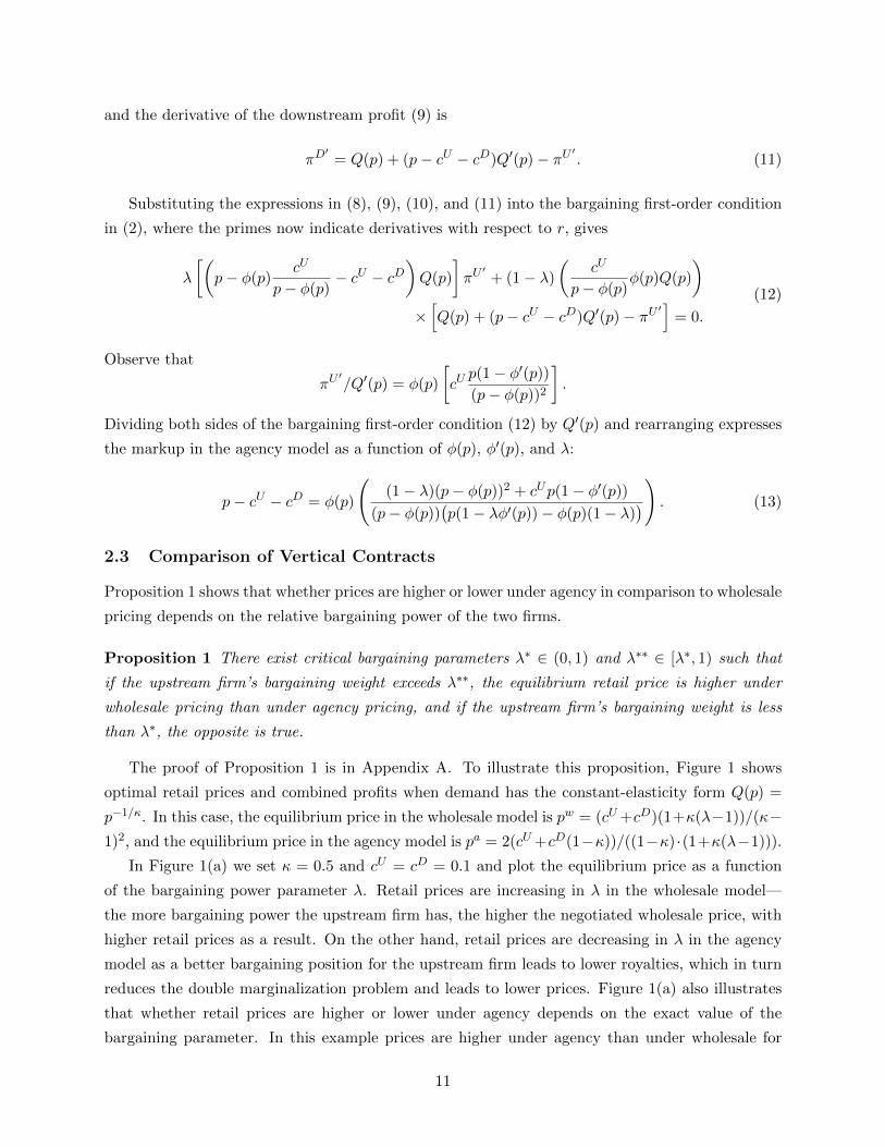
The proof of Proposition 1 is in Appendix A. To illustrate this proposition, Figure 1 shows
optimal retail prices and combined profits when demand has the constant-elasticity form Q(p) =
p−1/κ. In this case, the equilibrium price in the wholesale model is pw = (cU+cD)(1+κ(λ−1))/(κ−1)2, and the equilibrium price in the agency model is pa = 2(cU +cD(1−κ))/((1−κ) ·(1+κ(λ−1))).
In Figure 1(a) we set κ = 0.5 and cU = cD = 0.1 and plot the equilibrium price as a function
of the bargaining power parameter λ. Retail prices are increasing in λ in the wholesale model—
the more bargaining power the upstream firm has, the higher the negotiated wholesale price, with
higher retail prices as a result. On the other hand, retail prices are decreasing in λ in the agency
model as a better bargaining position for the upstream firm leads to lower royalties, which in turn
reduces the double marginalization problem and leads to lower prices. Figure 1(a) also illustrates
that whether retail prices are higher or lower under agency depends on the exact value of the
bargaining parameter. In this example prices are higher under agency than under wholesale for
11

Figure 1: Retail prices and combined profit as a function of bargaining power
(a) Retail price
(b) Combined profits
Notes: Retail price (figure a) and combined upstream and downstream profit (figure b) as a function of the bargaining weightfor the wholesale model and agency model. Demand is Q(p) = p−2 and cU = cD = 0.1.
bargaining power parameters that are less than 0.23 and lower otherwise. Also note that in the
case of take-it or leave-it offers, which corresponds to λ = 1 for the wholesale model and λ = 0 for
the agency model, prices under wholesale are higher than prices under agency.11
Figure 1(b) shows the combined profits of the upstream and downstream firm as a function of
the bargaining power parameter for each of the two models. For this particular example, the joint
firm profits are maximized under the agency model when the firms share equal bargaining power.
However, under the wholesale model joint profits are maximized when the downstream firm has all
the bargaining power. The latter happens because when the downstream firm has all the bargaining
power, it will demand a wholesale price that equals the marginal cost of the upstream firm, which
completely eliminates the double marginalization problem and maximizes joint firm profits.
Figure 2(a) compares the upstream firm’s profit under the two types of vertical contracts for the
same demand parameters, whereas 2(b) makes the same comparison for the downstream firm. In
this example, the upstream firm always prefers agency pricing whereas the downstream firm prefers
wholesale pricing. The opposite is true when firms use take-it or leave-it offers in which the party
that does not control retail prices has all bilateral bargaining power, i.e., λ = 1 under wholesale
pricing and λ = 0 under agency pricing. It follows that with take-it or leave-it offers, transitioning
to agency means higher profits for the downstream firm and lower profits for the upstream firm
(see also Proposition 3 of Johnson, 2017).
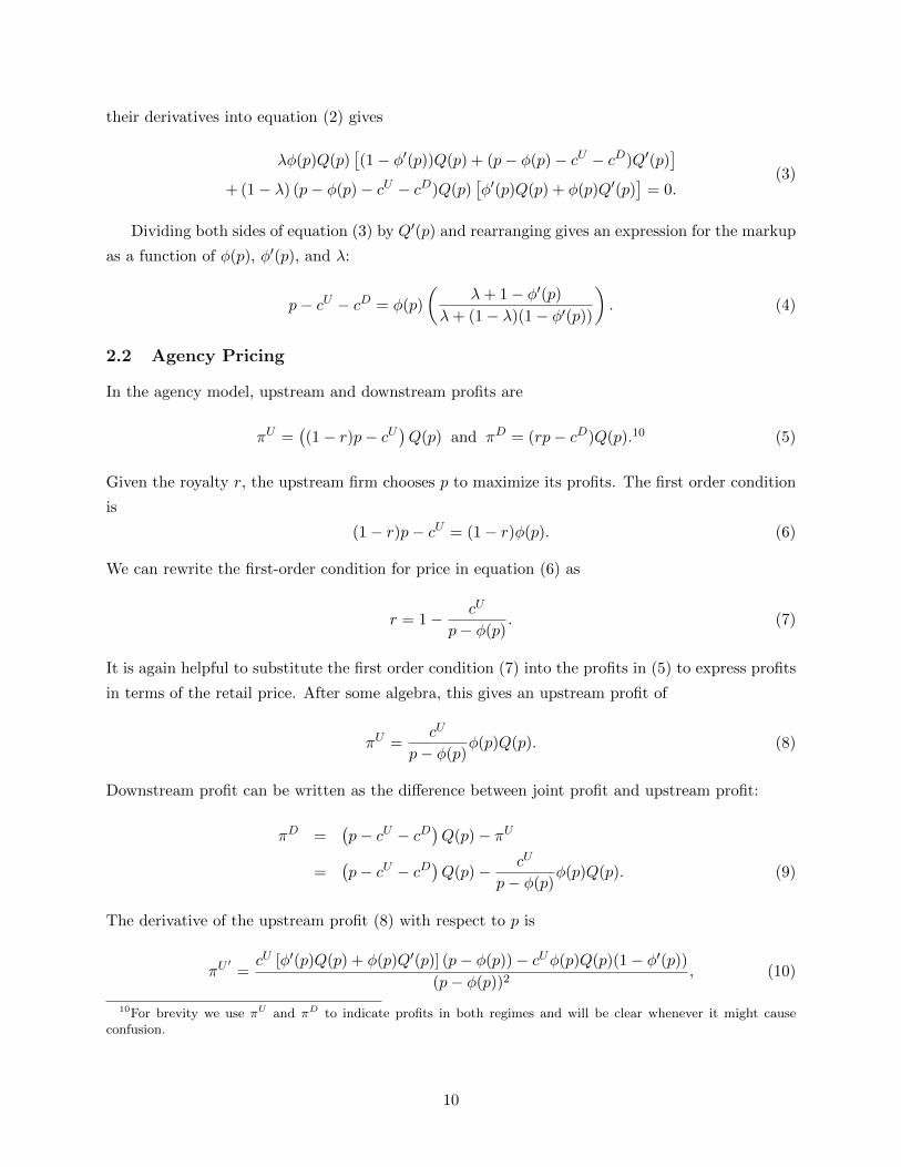
Note that in our bargaining model it is not always the case that the downstream firm prefers
wholesale agreements. Figures 3(a) and 3(b) show profits as a function of the bargaining weight
when the marginal cost for the upstream firm is 0.6 instead of 0.1—for intermediate values of the
bargaining parameter, both firms now prefer agency pricing.
11This result is consistent with the conditions of Lemma 2 of Johnson (2017) for lower retail prices under the agencymodel compared to the wholesale model.
12

Figure 2: Upstream and downstream profits as a function of bargaining power
(a) Upstream profits
(b) Downstream profits
Notes: Upstream profits (figure a) and downstream profits (figure b) as a function of the bargaining weight for the wholesalemodel and agency model. Demand is Q(p) = p−2 and cU = cD = 0.1.
3 Empirical Model
To make the model amendable for estimation, we extend the model to allow for multiple upstream
and downstream firms, as well as multi-product firms. In addition, we model consumer demand
using a logit discrete choice framework. In this section, we derive the equilibrium conditions of the
model.
3.1 Demand
We consider an industry with multiple upstream suppliers where each produces one or more goods
and sells a set of these goods non-exclusively through multiple downstream retailers. Upstream
producers can sell the same good through different retailers and retailers can sell goods of different
suppliers. We define a product as a good-retailer pair. That is, a product is a specific good sold
by a specific retailer. This means that product j sold by one retailer may be the same good as
product k sold by another retailer. The idea is that different good-retailer pairs (different products)
represent different points in product space. The utility consumer i derives from product j is given
by
uij = α log(pj) + x′jβ + ξj + εij , (14)
where pj is the price of product j, xj and ξj are observed and unobserved characteristics of product
j, α and β are demand parameters, and εij is a consumer-product specific utility shock. We allow for
an outside option with utility ui0 = εij . Assuming εij follows a Type I Extreme Value distribution,
and letting δj = α log(pj) + x′jβ + ξj , the market share of product j is
sj(p) =exp(δj)
1 +∑N
k=1 exp(δk).
13
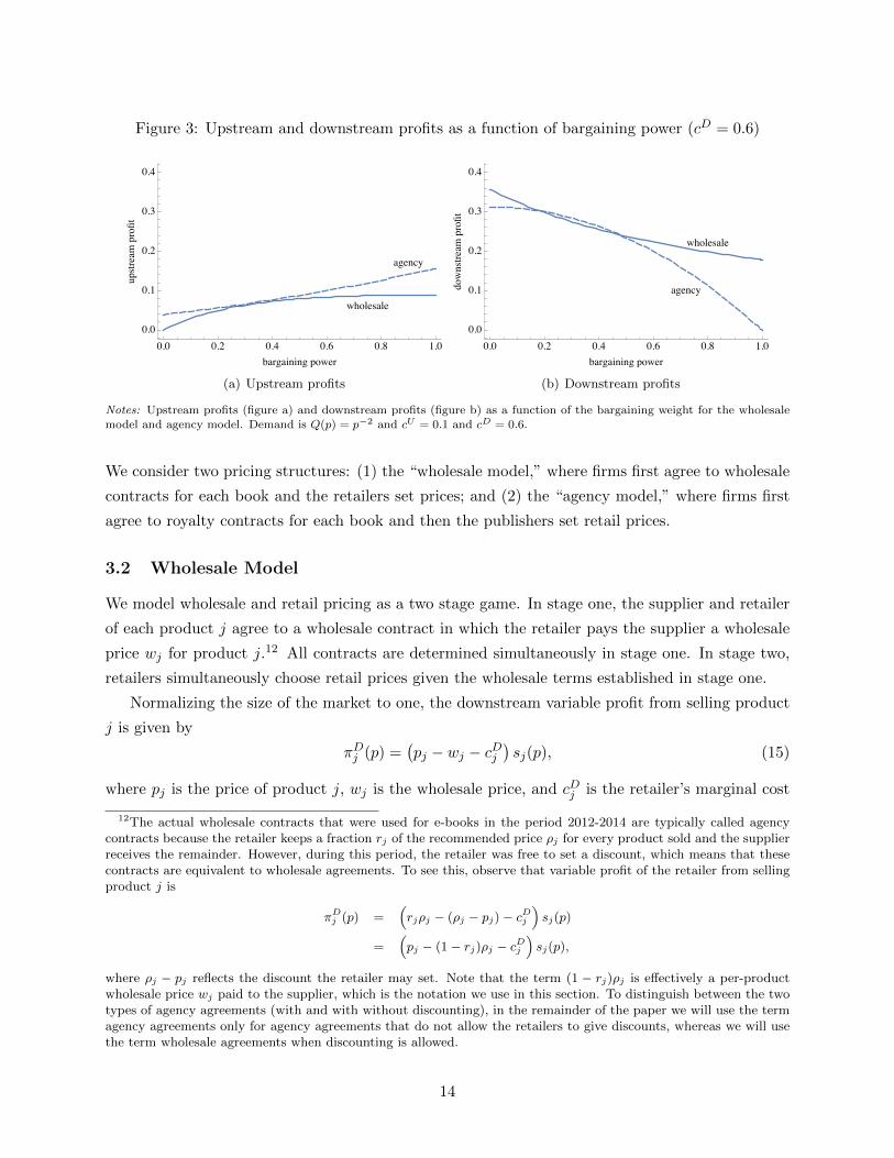
Figure 3: Upstream and downstream profits as a function of bargaining power (cD = 0.6)
(a) Upstream profits
(b) Downstream profits
Notes: Upstream profits (figure a) and downstream profits (figure b) as a function of the bargaining weight for the wholesalemodel and agency model. Demand is Q(p) = p−2 and cU = 0.1 and cD = 0.6.
We consider two pricing structures: (1) the “wholesale model,” where firms first agree to wholesale
contracts for each book and the retailers set prices; and (2) the “agency model,” where firms first
agree to royalty contracts for each book and then the publishers set retail prices.
3.2 Wholesale Model
We model wholesale and retail pricing as a two stage game. In stage one, the supplier and retailer
of each product j agree to a wholesale contract in which the retailer pays the supplier a wholesale
price wj for product j.12 All contracts are determined simultaneously in stage one. In stage two,
retailers simultaneously choose retail prices given the wholesale terms established in stage one.
Normalizing the size of the market to one, the downstream variable profit from selling product
j is given by
πDj (p) =(pj − wj − cDj
)sj(p), (15)
where pj is the price of product j, wj is the wholesale price, and cDj is the retailer’s marginal cost
12The actual wholesale contracts that were used for e-books in the period 2012-2014 are typically called agencycontracts because the retailer keeps a fraction rj of the recommended price ρj for every product sold and the supplierreceives the remainder. However, during this period, the retailer was free to set a discount, which means that thesecontracts are equivalent to wholesale agreements. To see this, observe that variable profit of the retailer from sellingproduct j is
πDj (p) =
(rjρj − (ρj − pj)− cDj
)sj(p)
=(pj − (1− rj)ρj − cDj
)sj(p),
where ρj − pj reflects the discount the retailer may set. Note that the term (1 − rj)ρj is effectively a per-productwholesale price wj paid to the supplier, which is the notation we use in this section. To distinguish between the twotypes of agency agreements (with and with without discounting), in the remainder of the paper we will use the termagency agreements only for agency agreements that do not allow the retailers to give discounts, whereas we will usethe term wholesale agreements when discounting is allowed.
14

of product j. The upstream variable profit from selling j is
πUj (p) =(wj − cUj
)sj(p), (16)
where cUj is the upstream supplier’s marginal cost of product j. The variable joint profit of the
supplier and retailer associated with product j is πJj = (pj − cDj − cUj )sj(p).
Downstream Market
Overall profits of the retailer that sells products in the set ΩD are given by
πD =∑j∈ΩD
(pj − wj − cDj
)sj(p).
We assume a pure-strategy Nash equilibrium in retail prices. The first-order condition for product
j is given by
sj +∑k∈ΩD
mDk
∂sk∂pj
= 0, (17)
where mDk = pk − wk − cDk is the downstream margin on product k. The derivative of the market
share of product k with respect to price pj is given by
∂sk∂pj
=
αsk (1− sk) /pk if k = j;
−αsjsk/pj if k 6= j.(18)
Upstream Market
We assume that wholesale prices are the outcome of a bilateral bargaining process between suppliers
and retailers, and separate wholesale prices are chosen for each product. Overall profits of an
upstream firm that sells products in the set ΩU are given by
πU =∑j∈ΩU
mUj sj(p),
where mUj = wj − cUj is the upstream margin for product j and cUj is the upstream firm’s marginal
cost for product j.
We assume that wholesale prices are determined through simultaneous Nash bargaining (“Nash-
in-Nash” bargaining) between the upstream and downstream firm associated with each product.
The Nash product for downstream firm d and upstream firm u is
NPdu(wdu;w−du) =(πU − dUdu
)λ (πD − dDdu
)1−λ, (19)
where wdu is the vector of wholesale prices of the products associated with the upstream-downstream
15

pair du, w−du is the vector of wholesale prices for products associated with other upstream-
downstream pairs, dUdu and dDdu are disagreement payoffs (discussed below), and λ ∈ [0, 1] is the
bargaining weight of upstream firm u. Although we do not index λ to keep the notation simple,
in our empirical application we allow λ to vary across supplier-retailer pairs. The Nash-in-Nash
bargaining solution is the vector of wholesale prices for all products such that wdu maximizes
NPdu for all upstream-downstream pairs du, given the results of the negotiations between other
upstream-downstream pairs.
Following Horn and Wolinsky (1988) and Crawford and Yurukoglu (2012), we assume rival firms
do not observe a bargaining breakdown, which means that rival firms do not adjust input or retail
prices if negotiations between a specific upstream-downstream pair fail.13 However, we do allow
market shares to adjust in case of disagreement. Specifically, we assume disagreement payoffs for
each du combination are given by
dUdu =∑
k∈ΩU\k∈du
mUk s−duk and dDdu =
∑k∈ΩD\k∈du
mDk s−duk .
In these expressions, s−duk is defined as the (counterfactual) market share for product k when
products of du are not offered, i.e.,
s−duk =exp(δk)
1 +∑
l∈Jg\l∈du exp(δl). (20)
So the disagreement payoff for the pair du consists of the profits for d from products not supplied
by u and profits for u for products sold by other retailers that are not available at retailer d,
considering that the demand for products −du may have increased as a result of the products du
not being sold.
The bargaining first-order condition is found by setting the derivative of equation (19) with
respect to wdu equal to zero for all products that belong to the set of products offered by each du
combination. Let j be such a product. The first-order condition for product j is
λ(πU − dUdu
)λ−1 (πD − dDdu
)1−λ ∂πU∂wj
+ (1− λ)(πU − dUdu
)λ (πD − dDdu
)−λ ∂πD∂wj
= 0. (21)
Since the Nash bargaining model defines an equilibrium payment for the set of products sold (and
not just for an individual product j), in this first-order condition πU and πD are the total profits
13Iozzi and Valletti (2014) show in a setting with one upstream firm and two downstream firms that the disagreementpayoff will depend on whether breakdowns are observable or not by the other downstream firm, which in turn may haveimplications for how input prices are determined. Crawford and Yurukoglu (2012) point out that an alternative modelin which other firms renegotiate based on disagreeing pairs dropping out is computationally much more challenging,and therefore estimate the simpler model in which breakdowns are unobservable by other firms.
16

of the upstream and downstream firm. Equation (21) can be simplified to
λ(πD − dDdu
) ∂πU∂wj
+ (1− λ)(πU − dUdu
) ∂πD∂wj
= 0. (22)
The partial derivatives ∂πU/∂wj and ∂πD/∂wj are given by
∂πU
∂wj=∑k∈ΩU
dπUkdwj
and∂πD
∂wj=∑k∈ΩD
dπDkdwj
,
where dπUk /dwj and dπDk /dwj are the total derivatives of πUk and πDk with respect to wj . These
total derivatives include the direct effect of wj on the profits as well as an indirect effect that comes
through changes in equilibrium prices p∗(w) and are derived in Appendix B.14 Condition (22)
together with condition (17) yield the equilibrium wholesale input prices and retail prices.
3.3 Agency Model
In the agency model, retail prices are set by the upstream suppliers, while the retailers obtain a
royalty rj . The variable profit of the retailer from selling product j is
πDj (p) =(rjpj − cDj
)sj(p).
The upstream variable profit from selling product j is
πUj (p) =((1− rj)pj − cUj
)sj(p).
The variable joint profit of the supplier and retailer associated with product j is πJj = (pj − cDj −cUj )sj(p).
Upstream Market
In the agency model, the upstream supplier determines the retail price pj . Overall profits of the
supplier that sells products in the set ΩU are given by
πU =∑j∈ΩU
((1− rj)pj − cUj
)sj(p).
14An alternative approach, which is used in Draganska, Klapper, and Villas-Boas (2010) and Ho and Lee (2017),assumes retail prices and input prices are simultaneously determined, which allows one to treat retail prices as fixed.In addition to treating the retail prices as fixed (which does not mean that retail price are independent of equilibriumretail prices), this literature also assumes that the derivative of the disagreement payoff with respect to input pricesis zero. While we depart from this literature by assuming input prices are determined taking into account that retailprices may change in response (i.e., we allow for a non-zero derivative of retail prices with respect to input prices), wedo keep the assumption that there are no disagreement payoff derivatives with respect to input prices. This impliesthat even if a firm is involved in multiple contract negotiations, it will treat each separately. As pointed out by Sheuand Taragin (2021), this assumption is important for maintaining tractability.
17

As in the wholesale model, we assume a pure-strategy Nash equilibrium in retail prices. The
first-order condition for product j is
(1− rj)sj +∑k∈ΩU
mUk
∂sk∂pj
= 0, (23)
where mUk = (1− rj)pj − cUj is the upstream margin on product k and the derivative of the market
share of product k with respect to pj is given by equation (18).
Downstream Market
The Nash bargaining solution is a vector of royalties that maximizes the Nash product,
NPdu(rdu; r−du) =(πU − dUdu
)λ (πD − dDdu
)1−λfor each upstream-downstream pair du, where rdu and r−du are vectors of royalties for the pairs
du and −du, respectively. The bargaining first-order condition is found by setting the derivative of
NPdu with respect to rdu equal to zero for all products that belong to the set of products offered
by each du combination. The bargaining first-order condition for one such product—product j—is
found by setting the derivative of the Nash product with respect to rj equal to zero, and can be
simplified to
λ(πD − dDdu
) ∂πU∂rj
+ (1− λ)(πU − dUdu
) ∂πD∂rj
= 0. (24)
Similar to the wholesale model, πU and πD are not just the profits for product j, but the total
profits of the firms. The partial derivatives ∂πU/∂rj and ∂πD/∂rj are given by
∂πU
∂rj=∑k∈ΩU
dπUkdrj
and∂πD
∂rj=∑k∈ΩD
dπDkdrj
,
where dπUk /drj and dπDk /drj are the total derivatives of πUk and πDk with respect to rj . These
total derivatives include the direct effect of rj on the profits as well as an indirect effect that comes
through changes in equilibrium prices p∗(r) and are derived in Appendix B. Condition (24) together
with condition (23) yield the equilibrium agency royalties and retail prices.
Upstream-Downstream–Specific Royalties. The analysis above assumes that a separate royalty
is set for every product, whereas we assume one royalty for each upstream-downstream pair when
structurally estimating the model. Modifying the analysis to allow for a setting in which each
upstream firm and retailer choose a single royalty for all of the upstream firm’s products carried
by the retailer is relatively straightforward. In bargaining over the profit-maximizing royalty to
set, retailer d and upstream firm u recognize that a change in royalty rj changes the royalties for
the other products from upstream firm u that are carried by retailer d by the same amount. The
first-order condition that reflects this behavior sets the sum of the derivatives in equation (24)
18

across the products sold by the pair du equal to zero and evaluates this sum at a common royalty,
rdu. That is, ∑j∈du
∂NPdu∂rj
∣∣∣∣∣rj=rdu ∀ j∈du, ∀du
= 0, for all du. (25)
The components of the left hand side of equation (25) are the same as the components of equation
(24).
4 Vertical Contracts in the E-Book Industry
In this section we focus on vertical contracts in the e-book industry. We first provide a description
of important changes in the contracts between upstream book publishers and downstream book
retailers. We then use a large dataset on retail prices in the period 2014-2015 to show how retail
prices changed at Amazon and Barnes & Noble as a result of the switch from wholesale to agency
contracts between publishers and bookstores. This transition to agency occurred after a period of
intense bilateral bargaining between retailers and publishers.
4.1 Background
Initially e-books were sold using wholesale contracts. Publishers would set a list price for the e-book
and would sell the book to a retailer for roughly half the list price. The retailer then would set a
retail price at which to sell the product to the consumers. This vertical contract changed in 2010
with the introduction of the iPad when Apple, together with five of the (then) Big Six publishers,
developed the agency model to sell e-books at the iPad’s new iBookstore. Publisher’s welcomed
Apple’s entrance to the e-book industry to provide a counterweight to Amazon’s dominance and saw
it as an opportunity to increase retail prices. Publishers believed that low e-book prices, especially
Amazon’s pricing of $9.99 for new releases, cannibalized hardcover sales and eroded consumers’
perception of a book’s value. As an MFN clause required the publishers to match retail prices
at the iBookstore to the lowest price retailer, publishers compelled Amazon to adopt the agency
model. Furthermore, the agency contracts included a mapping between list prices of newly released
hardcover titles and the agency retail prices for the corresponding e-books, where this mapping
was virtually identical across publishers.15 The switch from wholesale to agency contracts led to
an immediate increase in retail prices.
In 2012 the US Department of Justice sued Apple and the publishers for conspiring to raise
the prices of e-books. Three of the publishers settled right away, and the other two followed in
early 2013. As part of the settlement agreement the publishers could not set retail prices for a
period of two years.16 Moreover, the retail price most-favored nation clauses that were seen as
15The two basic price tiers were $12.99 for hardcover prices between $25 and $27.50 and $14.99 for hardcover pricesbetween $27.51 and $30.
16Note that termination dates of the bans were intentionally staggered to minimize the likelihood of collusive action
19

fundamental for making the switch to the agency model, were banned for a period of five years.17
The U.S. district court argued that the two-year ban on agency and the five-year ban on retail price
MFNs was necessary to provide a reset of the bilateral bargaining relationship between retailers
and publishers. Apple did not settle, but eventually lost the case after further appeals. As part
of the federal court’s injunction, which went into effect in October 2013, Apple could net enter
agency agreements with the publishers that were part of the lawsuit, with expiration dates ranging
from 24 months for agreements with Hachette to 48 months for agreements with Macmillan.18 De
los Santos and Wildenbeest (2017) show that the transition from agency to wholesale contracts
following the ban resulted in an 18 percent decrease in retail prices at Amazon and 8 percent at
Barnes & Noble.
Table 1: New contract announcement and switch dates for Amazon
Start of the New agency Amazon switchagency ban agreement announcement to agency
Simon & Schuster Dec 17, 2012 Oct 20, 2014 Jan 01, 2015Hachette Dec 04, 2012 Nov 13, 2014 Feb 01, 2015Macmillan Apr 04, 2013 Dec 18, 2014 Jan 05, 2015Harper Collins Sep 10, 2012 Apr 13, 2015 Apr 15, 2015Penguin Random House Sep 01, 2013 Jun 18, 2015 Sep 01, 2015
Sources: The agency agreement announcement dates as well as approximate switch dateswere widely reported by several media outlets (including a series of articles by Jeffrey Tra-chtenberg in the Wall Street Journal). Actual switch dates are verified using screenshotsfrom Amazon, from which it can be inferred whether the price was set by the publisheror by Amazon. The dates of the start of the agency ban, which correspond to the switchto the wholesale model under the terms of the settlements, are taken from De los Santosand Wildenbeest (2017).
The first column in Table 1 displays the effective date of the start of the ban on agency contracts
observed in the period after the settlement with the DOJ for each of the now Big Five publishers (De
los Santos and Wildenbeest, 2017).19 The second column of Table 1 displays the dates when it was
at the time new contracts had to be negotiated.17Early 2017 Amazon agreed to stop enforcing e-book MFN clauses in Europe as part of a settlement with the
European Commission. Although there was a similar lawsuit in 2012 in Europe as in the United States, with similarsettlements (a two year ban on agency and five year ban on pricing MFNs), this does not necessarily imply thatAmazon was using retail price MFN clauses in their agreements with the publishers prior to 2017 in the UnitedStates. Even though Amazon was not part of the 2012 lawsuits, the publishers that were part of the lawsuit werebanned from using pricing MFNs for a period of five years, which effectively meant that also Amazon could also notuse price MFNs in their agreements with these publishers during this period. However, since publishers that werenot part of the lawsuit are not covered by the settlements, Amazon could have potentially used MFNs in contractswith other publishers. Moreover, the 2017 settlement agreement with the European Commission was about the useof MFNs in general, which includes other restrictive ebook contract clauses, such as the requirements to disclose toAmazon the terms of contracts with other retailers.
18According to the final judgment and order entering permanent injunction (see https://www.justice.gov/atr/case-document/file/486651/download), “Apple shall not enter into or maintain any agreement with a Publisher Defendantthat restricts, limits, or impedes Apple’s ability to set, alter, or reduce the Retail Price of any E-book or to offerprice discounts or any other form of promotions to encourage consumers to purchase one or more E-books.”
19Because of a merger between Penguin and Random House in July 2013, the Big Six was renamed the Big Five.Although Random House was not a conspirator defendant in the DOJ lawsuits, Random House adopted the termsof the settlement after the merger, which is prior to the sample period for this paper.
20

reported in the media that Amazon and each of the publishers had reached a bilateral agreement.
The third column displays the dates when new agency agreements took effect and the switch to
agency can be identified in the data. The table shows that even though each publisher announced
an agreement with Amazon prior to the end of the two-year ban, the actual implementation dates
of the new agreements varied between January and September of 2015, which means that most
agreements did not go into effect immediately.
Note that while the media has reported extensively on Amazon’s dealings with each of the
Big Five publishers, we were unable to find reports on new agency agreements between Barnes &
Noble and the publishers. Moreover, unlike Amazon, Barnes & Noble does not mention on a book’s
product page whether or not the price was set by the publisher. Nevertheless, the two-year ban on
agency went into effect the same time for e-books sold at both Amazon and Barnes & Noble, which
meant that contracts had to be renewed around the same time for both retailers. Moreover, new
selling terms for Harper Collins e-books went into effect at the same date for all retailers.20 We
therefore make the assumption that for each publisher, the switch at Barnes & Noble happened at
the same date as at Amazon. Also note that we exclude Apple from the analysis below, since it
was banned from using agency agreements for a much longer period than the other retailers and
therefore did not switch back to agency agreements during our sample period.
Figure 4: Amazon inventory and e-book pricing decisions
Hachette ---> agreement announcement
<--- Hachette agreementimplementation
<--- Start of the bargaing period
0.2
.4.6
.81
Perc
enta
ge o
f boo
ks in
sto
ck a
t Am
azon
01jan
2014
01feb
2014
01mar2
014
01ap
r2014
01may
2014
01jun
2014
01jul2
014
01au
g201
4
01se
p201
4
01oc
t2014
01no
v201
4
01de
c201
4
01jan
2015
01feb
2015
01mar2
015
01ap
r2015
01may
2015
01jun
2015
Date
Harper CollinsHachetteSimon and SchusterMacmillanPenguin Random House
(a) Book Inventory by publisher
Hachette ---> agreement announcement
<--- Hachette agreementimplementation
<--- Start of the bargaing period
88.
59
9.5
10Av
erag
e H
ache
tte E
-boo
ks P
rices
at A
maz
on
01jan
2014
01feb
2014
01mar2
014
01ap
r2014
01may
2014
01jun
2014
01jul2
014
01au
g201
4
01se
p201
4
01oc
t2014
01no
v201
4
01de
c201
4
01jan
2015
01feb
2015
01mar2
015
01ap
r2015
01may
2015
01jun
2015
Date
(b) Hachette e-book prices at Amazon
Notes: Figure (a) gives the percentage of printed books in stock at Amazon over time for each of the Big Five publishers.Figure (b) gives the average Hachette e-book price at Amazon over time.
20According to Publishers Lunch (https://lunch.publishersmarketplace.com/2015/04/harper-readies-return-to-full-agency), “Multiple retailers report that Harper has informed them their selling terms will change as of Tuesday, April14. (The change is actually effective midnight Pacific time, rather than Eastern. Amazon would be among thosecompanies that naturally end their business day on Pacific time.) Harper is requiring retailers to implement allprice changes within 24 hours. Going forward Harper will require that their e-books be sold at the publisher’s listedconsumer price, without any discounts.” The article also notes that “Harper’s notice to retailers is an ‘interim’measure, in advance of more permanent new agency contracts,” which means that even though other retailers couldno longer offer discounts, they could still negotiate new terms regarding agency royalties.
21

In the period leading to the expiration of the two-year ban on agency contracts, publishers and
retailers engaged in a relatively lengthy period of negotiations over the conditions under which the
publishers would regain control of retail prices. The negotiations between Amazon and Hachette
became well known publicly as they included various pressure tactics. Amazon reduced the in-
ventory, delayed delivery, increased e-book prices, and removed the pre-order button of Hachette
titles. Hachette started a public campaign to pressure Amazon, which included the involvement of
support of some of their bestselling writers. The dispute between Amazon and Hachette started
in February 2014 when Amazon did not allow customers to pre-order and reduced inventories of
newly released Hachette books. Figure 4(a) shows that the percentage of printed Hachette books
that were in stock at Amazon declined sharply from levels around 90 percent, which was similar
to books from other publishers, to around 20 percent in November 2014.21 After the agreement
was announced, the percentage of Hachette books in stock immediately returned to 80 percent,
which was similar to inventory levels at other large publishers. The figure also shows that there
was a gradual reduction of the percentage of books in stock for other Big Five publishers starting
from the beginning of the year 2014, particularly for Penguin Random House, which was the last
publisher to reach an agreement with Amazon. Figure 4(b) shows that e-book prices of Hachette
titles increased sharply at the same time of the inventory reduction from average price levels of
around $8 to $9 and continued increasing during the bargaining period up to levels around $10.
After the announcement of the agreement, Amazon dropped prices sharply to levels around $8.50.
Prices increased again after the implementation of the agency agreement which gave control of
retail prices to Hachette.
4.2 The Effect of the Switch to Agency on Retail Prices
In this section we use a large dataset on retail prices for e-books to study the price effects of
the switch to agency contracts. Our sample runs between November 5, 2014 (seven weeks before
the first Big Five publisher switched) and October 21, 2015 (seven weeks after the last Big Five
publisher switched) and consists of daily prices (obtained using a web scraper) for a large number
of e-book titles. All titles are new and former New York Times bestseller books. Books that appear
in the New York Times bestseller lists are added to the sample from the moment of the appearance
on the list.22 For a specific title we observe its retail price as well as sales rank at both Amazon and
Barnes & Noble. Moreover, we observe book characteristics such as publisher, number of pages, and
ratings and number of reviews at Amazon. For the analysis, we focus on the Big Five publishers
and aggregate the data to weekly observations. Table 2 summarizes the variables.
For the analysis in this section, we use a similar difference-in-differences (DID) approach as
21The data used to create Figures 4(a) and 4(b) contains the same e-book titles used in the analysis in the nextsubsection, but also includes observations prior to November 5, 2014 as well as stock information for the printedversion of the e-books in the main sample.
22We modified the collection method for technical reasons in July 21, 2015. Because of this, the number of bookswe could track was reduced and was restricted to mostly popular books, as defined by the sales rank.
22

Table 2: Summary statistics
Harper Simon & PenguinCollins Hachette Schuster Macmillan Random House
Price e-bookAmazon 9.98 9.46 11.30 9.68 9.28
(3.52) (2.57) (2.93) (2.81) (2.68)Barnes & Noble 11.17 10.07 11.68 9.98 11.16
(3.78) (2.64) (2.68) (2.72) (2.71)
Book characteristicsRatings 4.31 4.23 4.30 4.21 4.25
(0.37) (0.40) (0.39) (0.40) (0.39)Number of reviews 1022.19 1264.89 944.45 882.05 1205.53
(2300.17) (2152.31) (1528.53) (1478.83) (2792.97)Number of months 26.74 29.64 30.29 26.85 31.90
since release (23.34) (23.46) (28.45) (19.43) (41.12)Number of pages 374.62 394.39 383.56 396.54 398.20
(133.19) (134.90) (142.50) (152.95) (219.30)
Number of titles 381 316 419 252 1,326Number of observations 20,016 20,055 26,334 15,632 83,551
Notes: The table gives the mean of each variable, with standard deviations in parentheses.
in De los Santos and Wildenbeest (2017). But where De los Santos and Wildenbeest study the
transition from agency contracts to wholesale contracts that followed the Justice Department’s
lawsuit against the major publishers and Apple in 2012, we focus on the transition from wholesale
to agency that occurred after the two-year ban on agency had expired in the period 2014-2015. An
important difference is that during the first period several of the key players in the industry were
found to be colluding. Another important difference is that MFN clauses were not used during
the second agency period and therefore do not play a role explaining the higher agency prices, as
argued by Johnson (2017). Note that in Section 5.5 we make an explicit comparison between the
first agency period and the second agency period when discussing the results of a counterfactual
exercise to study the effects of MFN on agency prices.
As was shown in Table 1, new contracts were announced between Amazon and the major
publishers at different points in time, resulting in the staggering of the actual switching dates at
Amazon. We exploit this cross-publisher variation in the timing of the switch in a difference-in-
differences setup. Specifically, the baseline specification we estimate is
log(pricejt) = γ · agencyjt + β ·Xj + νp + νw + εjt, (26)
where pricejt is the e-book price of title j at time t, agencyjt is an indicator for whether at time t
title j was sold using an agency contract, Xj are book characteristics, and νp and νw are publisher
and week fixed effects. The difference-in-differences estimator is captured by γ and gives the price
effect of the switch to the agency model.
23

Table 3: Results difference-in-differences analysis
Amazon Barnes & NoblePublisher Book Publisher Book
fixed effects fixed effects fixed effects fixed effects
Difference-in-differences estimatorAgency 0.132 0.127 -0.015 -0.022
(0.008) (0.007) (0.006) (0.005)Agency × Harper Collins 0.139 0.118 -0.048 -0.066
(0.018) (0.015) (0.016) (0.011)Agency × Hachette 0.072 0.073 0.014 0.007
(0.013) (0.010) (0.012) (0.009)Agency × Simon & Schuster 0.126 0.138 -0.020 -0.014
(0.013) (0.012) (0.008) (0.006)Agency × Macmillan 0.097 0.078 -0.054 -0.077
(0.019) (0.019) (0.017) (0.017)Agency × Penguin Random House 0.246 0.258 0.053 0.058
(0.016) (0.014) (0.015) (0.009)
Other controlsRating 0.020 0.020 0.027 0.031 0.012 0.012 -0.018 -0.023
(0.013) (0.013) (0.016) (0.016) (0.012) (0.012) (0.015) (0.015)Months since release -0.002 -0.002 0.001 0.001 -0.001 -0.001 0.001 0.001
(0.000) (0.000) (0.000) (0.000) (0.000) (0.000) (0.000) (0.000)Pages 0.071 0.070 0.091 0.090
(0.050) (0.050) (0.049) (0.050)Constant 2.122 2.128 2.039 2.029 2.321 2.322 2.423 2.448
(0.059) (0.059) (0.069) (0.070) (0.055) (0.055) (0.064) (0.064)
R-squared 0.152 0.155 0.829 0.832 0.078 0.080 0.855 0.857Number of observations 75,842 75,842 75,841 75,841 76,649 76,649 76,624 76,624
Notes: Dependent variable is log(price). All specifications include week fixed effects. Standard errors (clustered by book) inparentheses. The number of pages is divided by thousand.
24

Table 4: Placebo tests on the effect of switch to agency on print book prices
Amazon Barnes & Noble
Difference-in-differences estimatorAgency -0.001 -0.003
(0.004) (0.003)Agency × Harper Collins -0.005 -0.011
(0.009) (0.007)Agency × Hachette -0.021 -0.010
(0.009) (0.005)Agency × Simon & Schuster 0.009 0.004
(0.007) (0.005)Agency × Macmillan 0.015 0.013
(0.008) (0.008)Agency × Penguin Random House 0.006
(0.020)
Other controlsRating -0.042 -0.040 0.015 0.016
(0.020) (0.016) (0.013) (0.013)Months since release 0.001 0.001 -0.002 -0.002
(0.000) (0.000) (0.000) (0.000)Constant 2.784 2.773 2.740 2.733
(0.085) (0.086) (0.055) (0.055)
R-squared 0.896 0.896 0.839 0.839Number of observations 75,818 75,818 67,267 67,267
Notes: Dependent variable is log(price) of the printed version of the e-book. Allspecifications include book and week fixed effects. Standard errors (clustered bybook) in parentheses.
Table 3 gives the main results for the difference-in-differences analysis. We estimate equation
(26) separately for Amazon and Barnes & Noble. For each retailer, we estimate a specification that
allows for publisher fixed effects and a specification that has book fixed effects. As can be seen
from Table 3, the difference-in-differences estimator is very similar across the two specifications.
For Amazon, the estimates imply that prices went up by approximately 14 percent as a result
of the switch from wholesale to agency; for Barnes & Noble prices went down by approximately
2 percent. Table 3 also shows the results for a specification in which we split out the effect by
publisher. Consider first Amazon. The results for the baseline specification show that the effect
is not the same across publishers: the percentage increase in e-book prices following the switch
ranges from 7 percent for Hachette to 28 percent for Penguin Random House. The findings for
books sold at Barnes & Noble are also mixed. Prices for Macmillan and Harper Collins titles
decreased following the switch to agency, while prices for books published by Penguin Random
House increased by approximately 5 percent. The evolution of prices for the publishers are also
shown in Figure 5, which show the average price changes at Amazon by publisher around the
agreement announcement (dotted vertical line) and the date of the switch to agency (solid vertical
line). The figures show jumps in prices for Amazon around the time of the switch, but much less
so for Barnes & Noble.
To analyze if the effects can be attributed to the switch from wholesale to agency model and
not to other shocks that may have occurred around the switching dates, we run a placebo test in
25

Figure 5: E-book prices at Amazon and Barnes & Noble by publisher
89
1011
1213
Aver
age
E-bo
ok P
rices
19no
v201
4
03de
c201
4
17de
c201
4
01jan
2015
15jan
2015
29jan
2015
12feb
2015
26feb
2015
12mar2
015
26mar2
015
09ap
r2015
23ap
r2015
07may
2015
21may
2015
04jun
2015
18jun
2015
02jul2
015
16jul2
015
30jul2
015
13au
g201
5
27au
g201
5
10se
p201
5
24se
p201
5
08oc
t2015
Date
AmazonBarnes & Noble
(a) Harper Collins
89
1011
1213
Aver
age
E-bo
ok P
rices
19no
v201
4
03de
c201
4
17de
c201
4
01jan
2015
15jan
2015
29jan
2015
12feb
2015
26feb
2015
12mar2
015
26mar2
015
09ap
r2015
23ap
r2015
07may
2015
21may
2015
04jun
2015
18jun
2015
02jul2
015
16jul2
015
30jul2
015
13au
g201
5
27au
g201
5
10se
p201
5
24se
p201
5
08oc
t2015
Date
AmazonBarnes & Noble
(b) Hachette
89
1011
1213
Aver
age
E-bo
ok P
rices
19no
v201
4
03de
c201
4
17de
c201
4
01jan
2015
15jan
2015
29jan
2015
12feb
2015
26feb
2015
12mar2
015
26mar2
015
09ap
r2015
23ap
r2015
07may
2015
21may
2015
04jun
2015
18jun
2015
02jul2
015
16jul2
015
30jul2
015
13au
g201
5
27au
g201
5
10se
p201
5
24se
p201
5
08oc
t2015
Date
AmazonBarnes & Noble
(c) Simon & Schuster
89
1011
1213
Aver
age
E-bo
ok P
rices
19no
v201
4
03de
c201
4
17de
c201
4
01jan
2015
15jan
2015
29jan
2015
12feb
2015
26feb
2015
12mar2
015
26mar2
015
09ap
r2015
23ap
r2015
07may
2015
21may
2015
04jun
2015
18jun
2015
02jul2
015
16jul2
015
30jul2
015
13au
g201
5
27au
g201
5
10se
p201
5
24se
p201
5
08oc
t2015
Date
AmazonBarnes & Noble
(d) Macmillan
89
1011
1213
Aver
age
E-bo
ok P
rices
19no
v201
4
03de
c201
4
17de
c201
4
01jan
2015
15jan
2015
29jan
2015
12feb
2015
26feb
2015
12mar2
015
26mar2
015
09ap
r2015
23ap
r2015
07may
2015
21may
2015
04jun
2015
18jun
2015
02jul2
015
16jul2
015
30jul2
015
13au
g201
5
27au
g201
5
10se
p201
5
24se
p201
5
08oc
t2015
Date
AmazonBarnes & Noble
(e) Penguin Random House
Notes: Average e-book prices at Amazon and Barnes & Noble by publisher.
which we replicate the analysis using prices for the printed version of the e-book. Since printed
titles remained under the wholesale model, one would not expect to see a significant change in
prices for those books. Table 4 shows the results for a specification that has book fixed effects in
which we do not make a distinction by publisher, as well as the results split out by publishers.
26

The table shows that if we look at the overall effect of the switch to agency, there is no effect at
both Amazon and Barnes & Noble. If we split out the effect by publisher, we find some effect for
Hachette titles, although the effect is very small and not very precisely estimated.
The results from the difference-in-differences analysis point to two important observations.
First, the effect of the switch to agency agreements was different for Amazon than for Barnes &
Noble. Second, there is heterogeneity in the magnitude of the effect across publishers. These results
are consistent with our theoretical and empirical framework discussed in Sections 2 and 3 for a situ-
ation in which different retailers and publishers have different relative bargaining power parameters
and, therefore, respond differently to a move from wholesale contracts to agency contracts.
5 Estimation of the Bargaining Model
5.1 Data
We use a subset of the data used in the previous section to estimate the structural model—for
the estimation of the wholesale model we use the first seven weeks of the sample, while we use
the last seven weeks of the sample for the estimation of the agency model. Table 5 provides
summary statistics of the main variables we use by publisher. Panel A of the table gives summary
statistics for the seven-week period in which wholesale agreements were used by all of the publishers
(November/December 2014) whereas panel B gives summary statistics for the seven-week period
in which agency agreements were used by all the Big Five publishers (September/October 2015).
As before, we use weekly observations. For both periods we use the 100 most popular titles in our
sample, using the restriction that for a title to be included, we need to have observations for both
Amazon and Barnes & Noble throughout the entire sample.23 In total we have 14 weeks of data,
which corresponds to a total of 2,800 weekly observations (1,400 for the wholesale period and 1,400
for the agency period). The largest Big Five publisher, Penguin Random House, represents most
of the observations in our sample. Macmillan is the smallest with 6 titles. As we lack quantity
data for each book title, we use the approach suggested by Chevalier and Goolsbee (2003) to infer
sales from the observed sales rank data (see Appendix D for details). A comparison of the average
prices under the two selling regimes indicates that even though average prices were $2.59 higher
at Barnes & Noble than at Amazon during the wholesale period, average prices under agency are
very similar across the retailers, despite the five-year ban on the use of retail price MFN clauses
during this period.
5.2 Estimation Approach
Our estimation approach is to jointly estimate demand and supply and to use covariance restrictions
to deal with endogeneity concerns (MacKay and Miller, 2021). The unobserved characteristic
23Unfortunately, we do not have data sales rank data for Apple, so we cannot include Apple when estimating themodel.
27

Table 5: Summary statistics
Panel A. Wholesale period Panel B. Agency periodHarper Hachette Simon & Mac- Penguin Harper Hachette Simon & Mac- PenguinCollins Schuster millan Random Collins Schuster millan Random
House House
Price e-bookAmazon 9.98 7.67 6.17 7.47 7.59 9.97 9.46 10.27 11.03 10.81
(3.86) (2.33) (2.18) (3.42) (2.42) (1.29) (2.06) (1.19) (3.16) (1.95)Barnes 11.38 9.47 10.66 11.44 10.13 10.03 9.46 10.66 11.03 10.82& Noble (3.39) (2.75) (0.73) (2.55) (1.97) (1.22) (2.05) (0.73) (3.16) (1.95)
Weekly salesAmazon 4,225 6,627 736 1,074 4,057 1,165 484 679 366 2,724
(5,891) (24,038) (585) (881) (14,717) (3,778) (318) (2,954) (205) (17,298)Barnes 1,557 1,040 128 144 520 269 316 107 149 390& Noble (2,864) (3,869) (168) (93) (1,373) (268) (346) (120) (153) (1,136)
Book characteristicsRatings 4.30 4.20 4.40 4.40 4.29 4.24 4.22 4.43 4.41 4.29
(0.25) (0.38) (0.16) (0.20) (0.32) (0.26) (0.34) (0.15) (0.20) (0.33)Months 12 21 32 25 48 22 31 42 35 58since release (10) (20) (18) (16) (84) (10) (20) (18) (16) (84)
Pages 401 443 497 499 506 401 443 497 499 506(76) (109) (207) (273) (229) (76) (109) (207) (273) (229)
Titles 7 18 8 6 61 7 18 8 6 61Observations 98 252 112 84 854 98 252 112 84 854
Notes: The table presents the means of each variable, with standard deviations in parentheses.
ξj in the utility function (14) captures unobserved quality, which is likely to be correlated with
a book’s price. Our main specification below includes product and store fixed effects, so the
product- and store-specific variation in unobserved quality that does not vary over time is captured
by these fixed effects. However, these fixed effects will not pick up variation in prices due to
differences in unobserved quality over time. For instance, a favorable review in Oprah’s Book Club
may lead to a sudden increase in demand and retail prices. The traditional approach to resolve
price endogeneity is to use supply-side instruments and estimate the demand side of the model
using instrumental variables. However, the BLP-type instruments that are typically used when
estimating demand (see Berry, Levinsohn, and Pakes, 1995) are difficult to apply in this context
since e-book attributes do not explain much of the variance in sales and demand. Hausmann-
type instruments are not suitable either since there is no regional price variation in this market.
Instead, we follow the approach suggested by MacKay and Miller (2021), which is to restrict the
covariance between unobserved demand and cost shocks to be zero. Intuitively, the supply side
model imposes restrictions on how prices respond to demand shocks, and by restricting how the
demand and supply unobservables move together, it is possible to obtain causal estimates of the
endogenous price parameter without needing supply-side instruments. Although an assumption of
zero correlation between the unobserved demand and cost shocks may seem ad hoc, we include
fixed effects in both the demand and cost function to make the zero-covariance restriction more
28

credible. For instance, a potential concern here is that books with greater unobserved quality may
also have higher marginal costs—the product fixed effects will absorb the quality component from
the demand and costs shocks, making the zero-correlation assumption more plausible.
The parameters to be estimated are the parameters of the demand and marginal cost functions,
as well as the bargaining parameters. Throughout the analysis, we assume the bargaining param-
eters do not change throughout the sample, i.e., we estimate one bargaining parameter for each
publisher-retailer combination (which does not depend on the type of vertical contract). In addition
to assuming the bargaining parameters do not vary with the type of vertical contract, we assume
that the demand parameters as well as the marginal cost parameters remain the same across the
two periods, which means that identification of the bargaining parameters is largely driven by the
change in prices we observe as a result of switching from the wholesale model to the agency model.
Start with the demand side of the model. Since we are assuming the model has a logit structure,
we can express demand for product j in period t as
log(sjt)− log(s0t)− α log(pjt) = Xjtβ + ξjt, (27)
where pjt is likely to be correlated with ξjt. Given α, the demand side residuals can be obtained
as the residuals of a regression of the left-hand side of this expression on Xjt.
Next, consider the supply side of the model. Since the retailers’ marginal costs are likely to be
negligible, we set the retailers’ marginal cost to zero.24 The combined upstream and downstream
markup of product j equals the difference between price and marginal cost, which means upstream
marginal cost cjt equals
cjt = pjt −mDjt −mU
jt,
where, depending on whether agency or wholesale agreements were used in period t, we use the
first-order conditions for the wholesale or agency period derived in Section 3 to solve for mDjt and
mUjt as a function of the parameters.
Consider first the wholesale model. The vector of downstream margins mD can be written as
mD = −(TD ·∆
)−1s, (28)
where TD is an ownership matrix whose (j, k)th element is 1 if products j and k are sold by the
same retailer and zero otherwise and ∆ is a matrix of market share derivatives with respect to
price whose (j, k)th element is given by ∂sk/∂pj in equation (18).25 The upstream margin when
wholesale contracts are used can be found by solving the equilibrium condition in equation (22) for
24Alternatively, a retailer’s marginal cost v can be estimated alongside the other parameters.25When using matrix notation, we use · to indicate an entrywise (Hadamard) product.
29
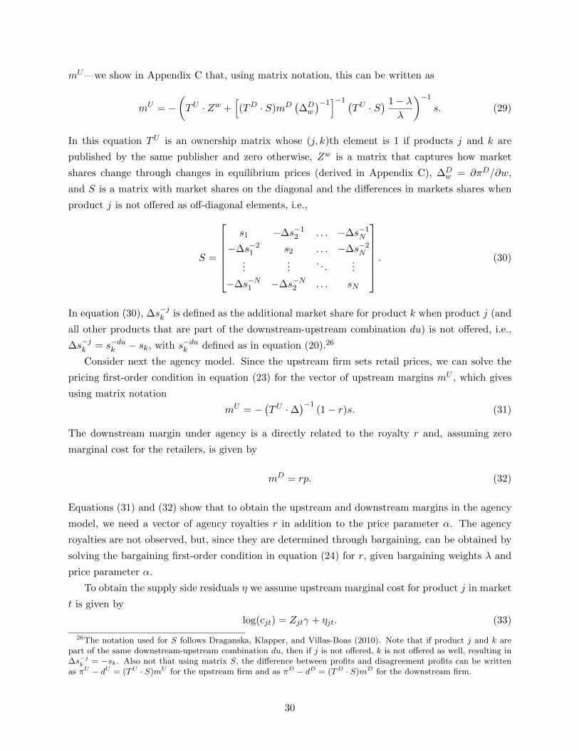
mU—we show in Appendix C that, using matrix notation, this can be written as
mU = −(TU · Zw +
[(TD · S)mD
(∆Dw
)−1]−1 (
TU · S) 1− λ
λ
)−1
s. (29)
In this equation TU is an ownership matrix whose (j, k)th element is 1 if products j and k are
published by the same publisher and zero otherwise, Zw is a matrix that captures how market
shares change through changes in equilibrium prices (derived in Appendix C), ∆Dw = ∂πD/∂w,
and S is a matrix with market shares on the diagonal and the differences in markets shares when
product j is not offered as off-diagonal elements, i.e.,
S =
s1 −∆s−1
2 . . . −∆s−1N
−∆s−21 s2 . . . −∆s−2
N...
.... . .
...
−∆s−N1 −∆s−N2 . . . sN
. (30)
In equation (30), ∆s−jk is defined as the additional market share for product k when product j (and
all other products that are part of the downstream-upstream combination du) is not offered, i.e.,
∆s−jk = s−duk − sk, with s−duk defined as in equation (20).26
Consider next the agency model. Since the upstream firm sets retail prices, we can solve the
pricing first-order condition in equation (23) for the vector of upstream margins mU , which gives
using matrix notation
mU = −(TU ·∆
)−1(1− r)s. (31)
The downstream margin under agency is a directly related to the royalty r and, assuming zero
marginal cost for the retailers, is given by
mD = rp. (32)
Equations (31) and (32) show that to obtain the upstream and downstream margins in the agency
model, we need a vector of agency royalties r in addition to the price parameter α. The agency
royalties are not observed, but, since they are determined through bargaining, can be obtained by
solving the bargaining first-order condition in equation (24) for r, given bargaining weights λ and
price parameter α.
To obtain the supply side residuals η we assume upstream marginal cost for product j in market
t is given by
log(cjt) = Zjtγ + ηjt. (33)
26The notation used for S follows Draganska, Klapper, and Villas-Boas (2010). Note that if product j and k arepart of the same downstream-upstream combination du, then if j is not offered, k is not offered as well, resulting in∆s−j
k = −sk. Also not that using matrix S, the difference between profits and disagreement profits can be writtenas πU − dU = (TU · S)mU for the upstream firm and as πD − dD = (TD · S)mD for the downstream firm.
30

Equations (27) and (33) give us the demand side residuals ξjt(α, β, λ;Xjt) and supply side residuals
ηjt(α, γ, λ;Xjt) given the data and the parameters of the model. Following MacKay and Miller
(2019), we use the following orthogonality condition for identification
Et[ξjt · ηjt] = 0 ∀j, k,
where the expectation is over markets. The corresponding empirical moments that are used to
estimate the parameters of the model σ (which includes α, β, γ, λ) by GMM are then
σ = arg minσ
1
J2
∑j,k
(1
T
∑t
ξjt(σ;Xjt) · ηjt(σ;Xjt)
)2 . (34)
Computational Details. Due to the inherent complexity of the bargaining first-order condition
in the agency model, solving this first-order condition for r has to be done numerically. Because
of this, it is computationally much faster to start from a vector of royalties (one for each retailer-
publisher pair) and to use the bargaining first-order condition to obtain the vector of bargaining
weights λ (again, one for each retailer-publisher pair) as a function of the agency royalties and the
other parameters of the model for which the bargaining first-order condition holds. Specifically,
solving equation (24) for (1− λ)/λ gives
1− λλ
= −(πD − dD)
(∂πD/∂r
)−1
(πU − dU ) (∂πU/∂r)−1 . (35)
Taking into account the ownership structure and using matrix notation, we can write πD − dD =
(TD · S)mD and πU − dU = (TU · S)mU . We can then write equation (35) more compactly using
matrix notation, i.e.,
1− λλ
=[(TU · S)mU
(∆Ur
)−1]−1
(TD · S)mD(∆Dr
)−1, (36)
where ∆Ur = ∂πU/∂r and ∆D
r = ∂πD/∂r. By reorganizing the bargaining first-order condition for
the agency model this way, we end up with a closed-form expression for the bargaining parameters
as a function of the price parameter α as well as the agency royalties r (see equation (A10) in
Appendix C). Then, when estimating the model, instead of starting from an initial vector of
bargaining parameters λ and solving for r, one can starting from an initial vector of agency royalties
r and solve for λ, which significantly speeds up estimation.27 Since we are assuming the bargaining
weights do not depend on the selling method, we can then use equation (36) to substitute for
(1− λ)/λ in equation (29).
27It is important to stress that starting from a vector of λ’s and using the bargaining first-order condition tonumerically solve for r (given the other parameters) is identical to proceeding the other way around, but takes muchlonger since the bargaining first-order condition has to be solved numerically.
31

5.3 Small Sample Performance
To investigate identification as well as small sample performance of our estimation procedure, we
run a Monte Carlo exercise. The setup of the experiment is as follows. We simulate two retailers
who each sell two products, where the two products are provided by two different upstream firms,
so there are four differentiated products in total. We let the firms compete for a number of periods,
where in half the periods retail and input prices are set according to the wholesale model and in
half the periods retail and input prices are set using the agency model. We assume disagreement
payoffs are zero when bargaining. Furthermore, we let consumer i’s indirect utility for product j
in period t be given by uijt = 10− 4 log(pjt) + ξjt + εijt, whereas product j’s marginal cost during
period t is given by log(cjt) = 1 + ηjt. We generate data assuming both demand and supply shocks
are uniform, with ξ ∼ U(0, 0.5) and η ∼ U(0, 0.5). Table 6 reports the mean and standard deviation
of the estimated parameters, where each column represents a different number of markets.
Table 6: Monte Carlo simulations
10 markets 40 markets 100 marketsVariable True Coeff. Std. Dev. Coeff. Std. Dev. Coeff. Std. Dev.
PANEL A. DEMAND MODEL ONLY (OLS)log(price) -4.000 -3.539 (0.333) -3.549 (0.159) -3.553 (0.099)
PANEL B. DEMAND AND SUPPLY MODELDemand parameters
log(price) -4.000 -4.300 (0.468) -4.045 (0.230) -3.987 (0.148)
Bargaining parameters Retailer 1 (R1)Upstream firm 1 (U1) 0.200 0.199 (0.074) 0.190 (0.065) 0.188 (0.063)Upstream firm 2 (U2) 0.300 0.306 (0.107) 0.289 (0.095) 0.287 (0.090)
Bargaining parameters Retailer 2 (R2)Upstream firm 1 (U1) 0.400 0.410 (0.110) 0.394 (0.099) 0.388 (0.095)Upstream firm 2 (U2) 0.250 0.253 (0.095) 0.238 (0.085) 0.235 (0.078)
Number of observations 40 160 400
Notes: Results for each column are based on 10,000 simulations. Utility is given by uijt = 10− 4 log(pjt) +ξjt+εijt and marginal cost by log(cjt) = 1+ηjt. Data is generated assuming ξ ∼ U(0, 0.5) and η ∼ U(0, 0.5).
Panel A of Table 6 shows the estimates when only the demand side is estimated, using OLS—
failing to deal with price endogeneity results in the price parameter being underestimated, even
when 400 observations are used, as in the last column of the table. Panel B shows that by jointly
estimating supply and demand using the cross-covariance restrictions approach, the bias in the
price parameter disappears. The average price parameter is relatively close to the true parameter
value even when the number of markets it small, and the standard deviation of the estimates
decreases in the number of observations used. Furthermore, the nonlinear bargaining parameters
are very close to the true parameter values even when data from only ten markets is used, and
the estimates become more precise when the number of markets increases. As argued before, the
identification of the bargaining parameters follows from observed changes in prices when switching
32

selling methods, and the Monte Carlo results show that using data from both pricing regimes
allows one to successfully pin down the bargaining parameters while simultaneously dealing with
price endogeneity, even in relatively small samples.
Figure 6: Simulated prices for each upstream-retailer pair
U1/R1 (λ=0.20)
U2/R1 (λ=0.30)
U1/R2 (λ=0.40)
U2/R2 (λ=0.25)
AGENCY ⟶⟵ WHOLESALE
1 2 3 4 5 6 7 8 9 10period9.0
9.2
9.4
9.6
9.8
10.0
10.2
10.4
price
Notes: Simulated prices for each upstream-retailer pair for the 10 period case (averaged across 10,000 simulations). Utility isgiven by uijt = 10− 4 log(pjt) + ξjt + εijt and marginal cost by log(cjt) = 1 + ηjt. Data is generated assuming ξ ∼ U(0, 0.5)and η ∼ U(0, 0.5). Demand and bargaining parameters are given by Panel B of the first column of Table 6.
The identification argument can also be seen from Figure 6, which shows simulated prices for
each upstream-retailer pair for the 10 period case (averaged across the 10,000 simulations). The
figure shows that for upstream-retailer pairs with a relatively low bargaining parameter (U1/R1
and U2/R2), prices increase when switching to agency, whereas prices remain constant (U2/R1)
or go down (U1/R2) for the upstream-retailer pairs that face higher values of their bargaining
parameter λ.
5.4 Parameter Estimates
Table 7 gives the parameter estimates for various specifications of the bargaining model. Specifica-
tion (A) of Table 7 gives estimates of the demand parameters as well as the bargaining parameters
when using publisher fixed effects in the demand equation. Other demand shifters we include are
the log of the price, the five-star rating of the title on Amazon, months since the title was released,
the number of pages, store fixed effects, and week fixed effects. As marginal cost shifters we include
book fixed effects. In specification (B) we use book fixed effects in the demand specification instead
of publisher fixed effects, which means we can no longer include the number of pages, but leave
everything else the same. In both specifications the price coefficient is estimated precisely, with
demand estimated to be slightly less elastic in specification (B) than (A). Rating has the expected
sign in both specifications, but is only estimated precisely in the specification that has book fixed
effects. Months since release and the number of pages do not appear to significantly affect the
33

Table 7: Parameter estimates of the bargaining model
(A) (B)Publisher Book
Fixed Effects Fixed EffectsVariable Coeff. Std. Err. Coeff. Std. Err.
Demand parameterslog(price) -2.066 (0.188) -1.805 (0.139)rating 0.481 (0.353) 1.603 (0.696)months since release -0.004 (0.002) -0.384 (0.361)number of pages 0.638 (0.543)
Bargaining parameters AmazonHarper Collins 0.352 (0.112) 0.347 (0.099)Hachette 0.239 (0.051) 0.256 (0.043)Simon & Schuster 0.037 (0.144) 0.103 (0.081)Macmillan 0.097 (0.142) 0.149 (0.091)Penguin Random House 0.153 (0.052) 0.188 (0.032)Average 0.176 0.208
Bargaining parameters Barnes & NobleHarper Collins 0.477 (0.100) 0.441 (0.080)Hachette 0.400 (0.035) 0.378 (0.027)Simon & Schuster 0.430 (0.125) 0.389 (0.077)Macmillan 0.460 (0.130) 0.418 (0.079)Penguin Random House 0.368 (0.022) 0.351 (0.020)Average 0.427 0.395
Objective function 0.020 0.007Own price elasticity -2.066 -1.804
Number of observations 2,800 2,800
Notes: Bootstrapped standard errors shown in parentheses (clustered bybook title). Demand specification includes store and week fixed effects.Marginal cost specification includes book fixed effects.
marginal utility of an e-book.
All of the estimated bargaining power parameters are less than a half, which, given our assump-
tion that the bargaining weights are not affected by the selling method, suggests the retailers have
more bargaining power than the publishers. The bargaining parameters for Amazon are generally
lower than those for Barnes & Noble, which is consistent with the results of the difference-in-
difference analysis in Section 4, which indicated a bigger switch-related price effect for Amazon
than for Barnes & Noble, and hence suggests relatively more bargaining power for Amazon than
for Barnes & Noble. However, there is substantial variation in the estimated bargaining parameters
across publishers, which to some extent can be explained by the magnitude of the price effects we
found in Section 4. Especially the estimated bargaining parameters for Barnes & Noble show a
clear relation with the results of the difference-in-differences analysis: for both Harper Collins and
Macmillan we found a negative price effect of the switch to agency, which indicates these publishers
having relatively more bargaining power, exactly as their above average bargaining weight estimates
show. The relation with the reduced-form findings is less clear for Amazon, although we do find
bargaining power for Simon & Schuster and Penguin Random House—the publishers for which we
found the biggest price effects—to be below-average.
34

Table 8: Royalty parameter estimates
Amazon Barnes & Noble Average
SPECIFICATION A. PUBLISHER FIXED EFFECTSHarper Collins 0.322 (0.064) 0.254 (0.061) 0.288Hachette 0.373 (0.036) 0.291 (0.042) 0.332Simon & Schuster 0.472 (0.065) 0.277 (0.044) 0.375Macmillan 0.441 (0.072) 0.262 (0.055) 0.352Penguin Random House 0.420 (0.028) 0.307 (0.039) 0.363Average 0.406 0.278 0.342
SPECIFICATION B. BOOK FIXED EFFECTSHarper Collins 0.371 (0.072) 0.311 (0.058) 0.341Hachette 0.418 (0.032) 0.346 (0.035) 0.382Simon & Schuster 0.504 (0.044) 0.339 (0.033) 0.422Macmillan 0.476 (0.056) 0.323 (0.041) 0.400Penguin Random House 0.461 (0.026) 0.361 (0.029) 0.411Average 0.446 0.336 0.391
Notes: Bootstrapped standard errors shown in parentheses (clustered by booktitle).
Table 8 gives the estimated royalty parameters during the agency period for the two specifica-
tions in Table 7. The average royalty share across retailers and publishers is 0.391 for the model
with book fixed effects and 0.342 for the model with publisher fixed effects, which is higher than the
30 percent that was typically used during the first agency period (between 2010 and 2012). Agency
royalties are higher at Amazon than Barnes & Noble, which is in line with Amazon’s more favorable
bargaining power estimates. Publishers with below average bargaining power tend to have lower
agency royalties, although a publisher’s bargaining position matters here too. For instance, despite
having lower than average bargaining weight, Penguin Random House has above average royalities,
which can be explained by Penguin’s better bargaining position due to its size relative to other
publishers (which affects its disagreement payoffs).28
Table 9 reports the implied margins for the bargaining model estimates reported in column (B)
of Table 7. The table reports figures for both the wholesale and agency model and shows that the
publishers’ margins went up for all of the publishers when switching to agency contracts. Amazon’s
average downstream margin also went up when switching to agency contracts, but Barnes & Noble’s
margins went down as a result of the switch. Note that higher margins (and possibly profits) for
Amazon are not inconsistent with the theoretical model of Section 2—Figure 3 illustrates this point
by showing that while upstream profits are higher under agency, whether downstream profits are
higher under agency depends on the bargaining power parameters.
28According to purchases made through outlets tracked by NPD BookScan, the ranking of the Big 5 publisher interms of units sold in 2016 is (1) Penguin Random House; (2) HarperCollins; (3) Simon & Schuster; (4) Hachette;and (5) Macmillan.
35

Table 9: Prices and margins
Panel A. Wholesale period Panel B. Agency periodRetail Down- Whole- Up- Mar- Retail Down- Whole- Up- Mar-price stream sale stream ginal price stream sale stream ginal
margin price margin cost margin price margin cost
RetailersAmazon 7.65 4.32 3.33 0.70 2.63 10.48 4.74 5.74 3.20 2.54Barnes & Noble 10.24 5.70 4.55 1.45 3.10 10.52 3.69 6.83 3.81 3.02
PublishersHarper Collins 10.68 5.97 4.71 1.57 3.14 10.00 3.41 6.59 3.66 2.94Hachette 8.57 4.80 3.77 1.09 2.67 9.46 3.61 5.85 3.24 2.61Simon & Schuster 8.55 4.79 3.76 0.95 2.81 10.47 4.40 6.07 3.36 2.70Macmillan 9.45 5.29 4.16 1.13 3.03 11.03 4.41 6.62 3.67 2.95Penguin Random House 8.86 4.96 3.90 1.02 2.88 10.82 4.44 6.37 3.56 2.81
Notes: Estimates are for specification (B) in Table 7.
Robustness
Table 10 gives estimates for alternative models and estimation approaches, all estimated using
book fixed effects in the demand side of the model. In column (A) of the table we allow for a more
flexible demand system that allows for different price coefficients for the two retailers. Our main
specification has a single price parameter, which means that if Amazon and Barnes & Noble cater
to consumers who differ in their price sensitivity, the difference in price sensitivity will be picked
up by the bargaining parameters. As shown by the price parameter estimates in column (A) of
Table 10, Barnes & Noble customers do appear to be less price sensitive on average than Amazon
customers, although the difference is small. The bargaining parameters are not much affected by
allowing for this additional layer of heterogeneity, although Barnes & Noble is now estimated to
have slightly more bargaining power on average than in our main specification.
In column (B) of Table 10 we estimate the model assuming the publishers make take-it or
leave-it offers in the wholesale model, and the retailers make take-it or leave-it offers in the agency
model. The estimated demand parameters for this specification indicate demand is slightly more
elastic, whereas the other demand parameters do not differ much from the ones estimated in column
(B) of Table 7. A comparison of the objective function values for the two specifications suggests
the bargaining model outperforms the take-it or leave-it model. However, the two models are non-
nested—the bargaining model assumes the bargaining parameters are constant across the two types
of vertical contracts, while with take-it or leave-it contracts the publishers have all the bargaining
power in the wholesale model (λ = 1) and retailers have all the bargaining power in the agency
model (λ = 0). To formally test which model gives the best fit to the data, we use the non-nested
test proposed by Rivers and Vuong (2002). The test statistic is −200.51 which means we can
strongly reject the take-it or leave-it model against the bargaining model.29
29The Rivers and Vuong (2002) statistic is calculated as TN = (√N/σN )(Q1 − Q2), where N is the number of
observations, Q1 and Q2 are the objective function values of the bargaining model and the take-it or leave-it model,
36

Table 10: Parameter estimates alternative supply side model and estimation approaches
(A) (B) (C) (D)Retailer-specific Take-it or Royalties Demand and supplyprice parameter leave-it contracts fixed to 0.30 separately
Variable Coeff. Std. Err. Coeff. Std. Err. Coeff. Std. Err. Coeff. Std. Err.
Demand parameterslog(price) -2.130 (0.182) -2.427 (0.082) -1.341 (0.178)
Amazon -1.726 (0.120)B&N -1.588 (0.096)
rating 1.606 (0.693) 1.607 (0.709) 1.612 (0.806) 1.888 (0.810)months since release -0.400 (0.373) -0.327 (0.326) -0.276 (0.439) -0.251 (0.089)
Bargaining parameters AmazonHarper Collins 0.333 (0.027) 0.287 (0.038) 0.277 (0.035)Hachette 0.249 (0.093) 0.280 (0.034) 0.225 (0.073)Simon & Schuster 0.108 (0.040) 0.283 (0.053) 0.133 (0.075)Macmillan 0.151 (0.081) 0.279 (0.080) 0.160 (0.025)Penguin Random House 0.187 (0.085) 0.288 (0.029) 0.193 (0.045)Average 0.206 0.283 0.197
Bargaining parameters Barnes & NobleHarper Collins 0.417 (0.028) 0.273 (0.030) 0.356 (0.014)Hachette 0.366 (0.065) 0.274 (0.024) 0.321 (0.083)Simon & Schuster 0.376 (0.022) 0.273 (0.047) 0.336 (0.074)Macmillan 0.399 (0.078) 0.273 (0.046) 0.350 (0.015)Penguin Random House 0.347 (0.075) 0.274 (0.031) 0.311 (0.009)Average 0.381 0.274 0.335
Objective function 0.007 0.016 0.014 0.051Own price elasticity -1.657 -2.130 -2.427 -1.341
Number of observations 2,800 2,800 2,800 2,800
Notes: Bargaining parameters are fixed to 1 for wholesale model and 0 for agency model in specification (A). Bootstrappedstandard errors shown in parentheses (clustered by book title), except for demand parameters in column (D), which areTSLS standard errors. Demand specifications include book, store, and week fixed effects. Marginal cost specificationincludes book fixed effects.
As shown in Table 8, the average royalty estimate in our main specification is 39 percent, which is
higher than the 30 percent that was used during the first agency period. To analyze how sensitive
our bargaining parameter estimates are to the royalty estimates, Column (C) of Table 10 gives
estimates of the demand and supply parameters of the model when we estimate the model using the
same covariance restrictions as we use for the main specification, but now fix the royalties for both
Amazon and Barnes & Noble to 30 percent instead of estimating them. Comparing the estimates
to those in specification (B) of Table 7, two things stand out. First of all, the estimated price
coefficient is more negative—everything else given, with more price sensitive consumers it becomes
optimal to set lower royalties. Secondly, the average estimated bargaining parameter increases for
Amazon, but decreases for Barnes & Noble, which corresponds to a decrease in bargaining power for
Amazon but an increase for Barnes & Noble. In comparison to the royalty estimates from the main
respectively, and σN is the estimated standard deviation of the difference between Q1 and Q2 (estimated using100 bootstrap replications). The Rivers and Vuong test statistic has to be evaluated against a standard normaldistribution, which, given the test-statistic of −200.51, results in a p value of 0.000, so we can strongly reject thetake-it or leave-it model against the bargaining model.
37

specification, Amazon’s royalty is substantially lower, which implies Amazon has less bargaining
power than in our main specification. In general, the lower the royalties, the more negative the
estimated price parameter and the higher the estimated bargaining weights. For instance, if both
retailers obtain a 20 percent royalty, the estimates price coefficient drops to -3.330 and the average
upstream bargaining parameter faced by Amazon increases from an average of 0.208 to 0.344.
In column (D) of Table 10, we estimate demand and supply separately. To estimate the demand
side we use two-stage least squares, using lagged prices as an instrument for prices. This instrument
has been used in other markets in which it is difficult to use traditional instruments such as the
market for console video games (Nair, 2007; Shiller, 2013) as well as online marketplaces (Jin, Lu,
Zhou, and Fang, 2021). As can be seen in column (D) of Table 10, the estimated price coefficient
decreases in magnitude in comparison to our main specification. Also shown in the table are
the estimated supply side parameters, which are estimated in a separate step by minimizing the
sum of squared residuals of the marginal cost equation, taking the demand parameters as given.
The estimated bargaining parameters are again close to those for the main model, which suggests
estimation of the supply side parameters of the model is robust to using a more traditional IV-based
approach to estimate the model.
Table 11: Supply side estimates for different price parameters
(A) (B) (C)
Variable Coeff. Std. Err. Coeff. Std. Err. Coeff. Std. Err.
Price parameterslog(price)
Amazon -1.800 -2.200 -2.200B&N -1.800 -1.800 -2.200
Bargaining parameters AmazonHarper Collins 0.340 (0.097) 0.353 (0.128) 0.353 (0.125)Hachette 0.249 (0.041) 0.234 (0.052) 0.232 (0.048)Simon & Schuster 0.086 (0.082) 0.011 (0.053) 0.011 (0.078)Macmillan 0.137 (0.086) 0.082 (0.079) 0.081 (0.090)Penguin Random House 0.180 (0.028) 0.131 (0.029) 0.134 (0.033)Average 0.199 0.162 0.162
Bargaining parameters Barnes & NobleHarper Collins 0.447 (0.076) 0.446 (0.074) 0.490 (0.102)Hachette 0.384 (0.024) 0.383 (0.023) 0.405 (0.032)Simon & Schuster 0.408 (0.098) 0.408 (0.089) 0.438 (0.111)Macmillan 0.433 (0.091) 0.432 (0.083) 0.471 (0.105)Penguin Random House 0.359 (0.019) 0.361 (0.019) 0.370 (0.022)Average 0.406 0.406 0.435
Objective function 0.042 0.036 0.041Own price elasticity -1.800 -2.000 -2.200
Number of observations 2,800 2,800 2,800
Notes: Bootstrapped standard errors shown in parentheses (clustered by book title).Marginal cost specification includes book fixed effects.
To get a better sense of how the uncertainty related to the price parameters affects the supply
side estimates, in Table 11 we take a different approach and calibrate the price coefficients instead of
38

estimating them. We then estimate the supply side model only by minimizing the sum of squared
(upstream) marginal cost residuals. In column (A) of this table we fix the price parameter to
−1.8 for both Amazon and Barnes & Noble, which corresponds to the estimate we obtained from
our main specification. Although the estimation approach is different (i.e., minimizing the sum
of squared marginal cost residuals instead of targeting zero cross-covariance between demand and
supply side residuals), we do get very similar bargaining parameter estimates. Next, we keep the
price parameter for Barnes & Noble fixed at −1.8, but change the coefficient for Amazon to −2.2,
which corresponds to Amazon’s internal estimate of the average price elasticity for e-books.30 As
shown in column (B) of the table, more elastic demand at Amazon leads to lower bargaining weight
estimates on average, which implies more bargaining power for Amazon. When changing both price
coefficients to −2.2, as in column (C) of the table, both Amazon and Barnes & Noble are estimated
to have more bargaining power relative to the publishers. Nevertheless, the differences with the
estimates for the main specification are relatively small, which suggests the supply side estimates
are relatively robust to variation in the price parameters.
5.5 Counterfactual Analysis of the Most Favored Nations Clause
The settlements between DOJ and the Big Five publishers in 2012 explicitly banned the use of
retail price MFN clauses for a period of five years. In this section we study what happens to agency
prices when retail price MFN clauses are reinstated, which starting in 2017 is again a possibility.
According to DOJ, the MFN clauses that were used during the initial switch to agency contracts in
2010 were essential for making the entire industry shift towards agency agreements, with the switch
from wholesale to agency leading to higher consumer prices. Even though the largest publishers
are again using the agency model and MFN clauses were not instrumental for making the switch
to this second period of agency pricing, this does not mean that MFN clauses are unlikely to have
a further impact on pricing once permitted again. The reason for this is that MFN guarantees a
retailer who prefers a higher royalty, if it raises the royalty for one publisher, the retail price will
remain the same relative to other retailers. This encourages retailers to push for higher royalties,
which results in higher retail prices (see also Johnson, 2017).
To simulate what happens to retail prices when MFN agreements are used, we use the estimates
from specification (B) of Table 7 to simulate equilibrium prices and royalties, using the restriction
that the same title should have the same prices at both Amazon and Barnes & Noble. This
restriction will not only affect the retail pricing first-order condition but also the bargaining first-
order condition, assuming that contracts between publishers and retailers are renegotiated. The
implications of using MFN on prices, royalties, margins, and profits are shown in Table 12. The
table shows that royalties increase across the board, with Barnes & Noble seeing the biggest changes
30According to a message from the Amazon Books Team to the reader published at readersunited.com in 2014, “forevery copy an e-book would sell at $14.99, it would sell 1.74 copies if priced at $9.99,” which implies an own-priceelasticity of %∆Q/%∆P = 74/(100× (−5/14.99)) = −2.2.
39

Table 12: Prices, royalties, margins, and profits MFN
No MFN MFNPrice Royalty Margin Profits Price Royalty Margin Profits
RetailersAmazon 10.51 0.451 4.75 586,661 11.29 0.476 5.15 561,508Barnes & Noble 10.54 0.351 3.70 84,267 11.29 0.455 6.05 122,063
PublishersHarper Collins 9.85 0.341 3.60 22,517 10.90 0.423 3.37 18,420Hachette 9.60 0.382 3.29 38,788 10.52 0.479 3.04 32,727Simon & Schuster 10.55 0.422 3.39 7,734 10.96 0.544 3.15 7,075Macmillan 11.32 0.400 3.77 12,102 12.87 0.508 3.96 9,836Penguin Random House 10.79 0.411 3.55 395,577 11.45 0.445 2.66 374,213
Notes: Estimates are based on the bargaining model estimates reported in specification (B) of Table 7. Figuresin the Margin columns reflect downstream margins for the retailers and upstream margins for the publishers.
among the retailers and Hachette, Simon & Schuster, and Macmillan among the publishers. Even
though retail prices go up as well, by an average of seven percent across titles, this price increase is
not enough to prevent margins from going down for all but one of the publishers. Moreover, there
is a lot of variation in price changes across the publishers, ranging from a sales-weighted average
price increase of 3 percent for Penguin Random House to 13 percent for Macmillan. Table 12 also
shows that publishers’ profits decrease, which is driven by the higher share of revenue going to
the retailers combined with higher retail prices. Overall retail profits are up when MFN clauses
are used, although only Barnes & Noble benefits from this increase. Moreover, combined industry
profits are down, so even though Barnes & Noble would benefits substantially from reinstatement
of MFN clauses, this might not be enough for MFN agreements to make a comeback.
Table 13: Most-favored nation clause difference-in-differences analysis
Amazon Barnes & NoblePublisher Book Publisher Book
fixed effects fixed effects fixed effects fixed effects
Difference-in-differences estimatorAgency 0.143 0.137 -0.023 -0.039
(0.009) (0.008) (0.007) (0.006)Agency × MFN 0.078 0.073 0.121 0.114
(0.013) (0.012) (0.015) (0.012)Other controls
Rating on Amazon 0.033 -0.023 0.045 -0.026(0.010) (0.010) (0.010) (0.008)
Months since release -0.002 0.002 -0.002 0.001(0.000) (0.000) (0.000) (0.000)
Number of pages 0.048 0.068(0.044) (0.043)
Constant 2.056 2.219 2.168 2.431(0.046) (0.040) (0.047) (0.032)
R-squared 0.161 0.675 0.074 0.653Number of observations 255,194 255,239 250,434 250,443
Notes: Dependent variable is log(price). All specifications include week fixed effects.Standard errors (clustered by book) in parentheses. The number of pages is divided bythousand.
40

Although for the main analysis we only include observations for the second period in which
the industry shifted to agency contracts (2014-2015), for some of the books in our sample we also
have price data for the first period in which agency contracts were used (2010-2012). Table 13
provides results using a similar difference-in-differences approach as in Section 4.2, but with the
sample expanded to include the first agency period. Since MFN clauses were used in first agency
period but not in the second, the expanded sample allows us to directly compare the effect of
MFN on agency prices. As shown by the estimate on the Agency × MFN coefficient, prices where
between 7 and 8 percent higher during the first agency period for Amazon, while 12 to 13 percent
higher for Barnes & Noble. Note that these differences are somewhat higher than predicted by the
counterfactual exercise. A potential explanation for the difference is the alleged collusion during
the first agency period, which is captured by the difference-in-difference comparison between the
two periods, but is not picked up by the counterfactual simulations. The higher price increase
in the first agency period is consistent with this, and also shows the usefulness of our structural
analysis, since it allows us to separate the effect of MFN from the effect of collusion.
6 Conclusions
In this paper we have studied the effects of the transition from wholesale contracts to agency
contracts in the e-book market that occurred in the period from 2014 to 2015. Using a difference-
in-differences analysis, we have shown that prices went up by 14 percent following the switch at
Amazon, but went down 2 percent at Barnes & Noble. We have theoretically shown that if an
upstream and downstream firm are bargaining over input prices, retail prices will be higher or
lower under agency depending on the relative bargaining power of the firms.
Our structural model extends this theoretical model to allow for competition among publishers
and retailers, multi-product firms, and logit demand. We have shown how to estimate this model
using sales rank data, prices, and book characteristics. Estimates of the bargaining model have
shown that the retailers have most of the bargaining power, although there are large differences
in estimated bargaining weights between retailer-publisher pairs. Moreover, the bargaining model
better fits the data than a model in which input prices are determined using take-it or leave-it
contracts. The results from a counterfactual analysis in which we reinstate MFN clauses lead to
changes in consumer prices of about seven percent. Nevertheless, the counterfactual analysis also
shows that adoption of MFN would lower profits of the publishers as well as Amazon, which might
be a contributing factor for why MFN contracts so far have not made a return.
What complicates our analysis of the market for e-books is that the objective function of the
publishers and retailers has not always been clear. Our structural model assumes static profit
maximization within a single market, which means complementaries with other products as well as
dynamic considerations are not directly taken into account. For instance, Amazon not only sells
e-books, but also the hardware that goes with it, which may affect pricing or royalty decisions
41

(see Gaudin and White, 2014). Dynamic competition could be important too, especially since
consumers may face switching costs when moving between the retailers’ different e-book platforms
(see Johnson, 2020). Furthermore, we know from the 2012 lawsuit that the publishers were mostly
concerned about how low e-book prices affected the market for hardcover books and supported
the move to agency despite earning less from agency contracts than they were from wholesale
contracts. Another limitation of our study is that litigation of the initial agency contracts has likely
affected subsequent developments in this industry, so our results may not necessarily generalize to
other contexts in which contracts are not litigated. Despite these limitations, our study shows
the importance of the interaction of bargaining power and contract types (agency or wholesale) in
determining retail prices.
References
Abhishek, Vibhanshu, Kinshuk Jerath, and Z. John Zhang: “Agency Selling or Reselling? Channel Structuresin Electronic Retailing,” Management Science 62, 2258–2280, 2015.
Bagnoli, Mark and Ted Bergstrom: “Log-concave Probability and Its Applications,” Economic Theory 26,445–469, 2005.
Baker, Jonathan: “Cartel Ringmaster or Competition Creator? The Ebooks Case Against Apple,” in JohnE. Kwoka Jr. and Lawrence J. White (Editors), The Antitrust Revolution, 7th edition, 2018.
Berry, Steven, James Levinsohn, and Ariel Pakes: “Automobile Prices in Market Equilibrium,” Econometrica63, 841–890, 1995.
Bonnet, Celine and Pierre Dubois: “Identifying Two Part Tariff Contracts with Buyer Power: EmpiricalEstimation on Food Retailing,” Mimeo, 2015.
Cachon, Gerard P. and Martin A. Lariviere: “Supply Chain Coordination with Revenue-Sharing Contracts:Strengths and Limitations.” Management Science 51, 30–44, 2005.
Carlton, Dennis W. and Jeffrey M. Perloff: Modern Industrial Organization, Pearson, 2004.
Chevalier, Judith and Austan Goolsbee: “Measuring Prices and Price Competition Online: Amazon.comand BarnesandNoble.com,” Quantitative Marketing and Economics 1, 203–222, 2003.
Collard-Wexler, Allan, Gautam Gowrisankaran, and Robin S. Lee: ““Nash-in-Nash” Bargaining: A Micro-foundation for Applied Work,” Journal of Political Economy 127, 163–195, 2019.
Condorelli, Daniele, Andrea Galeotti, and Vasiliki Skreta: “Selling through Referrals,” Journal of Economics& Management Strategy 27, 669–685, 2018.
Conlon, Christopher T. and Julie Holland Mortimer: “Efficiency and Foreclosure Effects of Vertical Rebates:Empirical Evidence,” forthcoming in the Journal of Political Economy.
Crawford, Gregory S. and Ali Yurukoglu: “The Welfare Effects of Bundling in Multichannel TelevisionMarkets,” American Economic Review 102, 643–685, 2012.
Crawford, Gregory S., Robin S. Lee, Michael D. Whinston, and Ali Yurukoglu: “The Welfare Effects ofVertical Integration in Multichannel Television Markets,” Econometrica 86, 891–954, 2018.
42

Davidson, Carl: “Multiunit Bargaining in Oligopolistic Industries,” Journal of Labor Economics 6, 397–422,1988.
De los Santos, Babur and Matthijs R. Wildenbeest: “E-book Pricing and Vertical Restraints,” QuantitativeMarketing and Economics 15, 85–122, 2017.
Dennis, Anthony J.: “Most Favored Nation Contract Clauses under the Antitrust Laws,” University ofDayton Law Review 20, 821–854, 1995.
Dobson, Paul W. and Michael Waterson: “Countervailing Power and Consumer Prices,” Economic Journal107, 418–430, 1997.
Donna, Javier D., Pedro Pereira, Andre Trindade, and Renan C. Yoshida: “Direct-to-Consumer Sales byManufacturers and Bargaining,” Mimeo, 2021.
Draganska, Michaela, Daniel Klapper, and Sofia B. Villas-Boas: “A Larger Slice or a Larger Pie? AnEmpirical Investigation of Bargaining Power in the Distribution Channel,” Marketing Science 29, 57–74, 2010.
Foros, Øystein, Hans Jarle Kind, and Greg Shaffer: “Apple’s Agency Model and the Role of Most-Favored-Nation Clauses,” RAND Journal of Economics 48, 673–703, 2017.
Gans, Joshua S.: “Mobile Application Pricing,” Information Economics and Policy 24, 52–59, 2012.
Gaudin, Germain and Alexander White: “On the Antitrust Economics of the Electronic Books Industry,”Mimeo, 2014.
Gilbert, Richard J.: “E-books: A Tale of Digital Disruption,” Journal of Economic Perspectives 29, 165–184,2015.
Gowrisankaran, Gautam, Aviv Nevo, and Robert Town: “Mergers When Prices Are Negotiated: Evidencefrom the Hospital Industry,” American Economic Review 105, 172–203, 2015.
Grennan, Matthew: “Price Discrimination and Bargaining: Empirical Evidence from Medical Devices,”American Economic Review 103, 145–177, 2013.
Ho, Kate and Robin S. Lee: “Insurer Competition in Health Care Markets,” Econometrica 85, 379–417,2017.
Ho, Kate and Robin S. Lee: “Equilibrium Provider Networks: Bargaining and Exclusion in Health CareMarkets,” American Economic Review 109, 473–522, 2019.
Horn, Henrick and Asher Wolinsky: “Bilateral Monopolies and Incentives for Merger,” RAND Journal ofEconomics 19, 408–419, 1988.
Hristakeva, Sylvia: “Vertical Contracts with Endogenous Product Selection: An Empirical Analysis ofVendor-Allowance Contracts,” Mimeo, 2020.
Iozzi, Alberto and Tommaso Valletti: “Vertical Bargaining and Countervailing Power,” American EconomicJournal: Microeconomics 6, 106–135, 2014.
Jin, Ginger Zhe, Zhentong Lu, Xiaolu Zhou, and Lu Fang: “Flagship Entry in Online Marketplaces,” Mimeo,2021.
Johnson, Justin: “The Agency Model and MFN Clauses,” Review of Economic Studies 84, 1151–1185, 2017.
Johnson, Justin: “The Agency and Wholesale Models in Electronic Content Markets,” International Journalof Industrial Organization 69, Article 102581, 2020.
43
Francine Lafontaine: “Agency Theory and Franchising: Some Empirical Results,” RAND Journal of Eco-nomics 23, 263–283, 1992.
Li, Hui: “Are E-Books a Different Channel? Multichannel Management of Digital Products,” QuantitativeMarketing and Economics 19, 179–225, 2021.
Lia, Jia and Charles C. Moul: “Who Should Handle Retail? Vertical Contracts, Customer Service, andSocial Welfare in a Chinese Mobile Phone Market,” International Journal of Industrial Organization39, 29–43, 2015.
MacKay, Alexander and Nathan H. Miller: “Estimating Models of Supply and Demand: Instruments andCovariance Restrictions,” Mimeo, 2021.
Mantovani, Andrea, Claudio Piga, and Carlo Reggiani: “Online Platform Price Parity Clauses: Evidencefrom the EU Booking.com Case,” European Economic Review 131, Article 103625, 2021.
Mortimer, Julie Holland: “Vertical Contracts in the Video Rental Industry,” Review of Economic Studies75, 165-199, 2008.
Nair, Harikesh: “Intertemporal Price Discrimination with Forward-Looking Consumers: Application to theUS Market for Console Video-Games,” Quantitative Marketing and Economics 5, 239–292, 2007.
Nash, John F.: “The Bargaining Problem,” Econometrica 18, 155–162, 1950.
O’Brien, Daniel P., “The Uniform Settlements Policy in International Telecommunications: A Noncoopera-tive Bargaining Model of Intermediate Product Third Degree Price Discrimination,” doctoral disserta-tion, Northwestern University, 1989.
O’Brien, Daniel P., “The Welfare Effects of Third-Degree Price Discrimination in Intermediate Good Mar-kets: The Case of Bargaining,” RAND Journal of Economics 45, 92–115, 2014.
O’Brien, Daniel P. and Greg Shaffer, “Bargaining, Bundling, and Clout: The Portfolio Effects of HorizontalMergers,” RAND Journal of Economics 36, 573–595, 2005
Reimers, Imke and Joel Waldfogel: “Throwing the Books at Them: Amazon’s Puzzling Long-Run PricingStrategy,” Southern Economic Journal 83, 869–885, 2017.
Rivers, Douglas and Quong Vuong: “Model Selection Tests for Nonlinear Dynamic Models,” EconometricsJournal 5, 1–39, 2002.
Rubinstein, Ariel: “Perfect Equilibrium in a Bargaining Model,” Econometrica 50, 97–109, 1982.
Sheu, Gloria and Charles Taragin: “Simulating Mergers in a Vertical Supply Chain with Bargaining,”forthcoming in RAND Journal of Economics, 2021.
Shiller, Benjamin R.: “Digital Distribution and the Prohibition of Resale Markets for Information Goods,”Quantitative Marketing and Economics 11, 403–435, 2013.
Villas-Boas, Sofia Berto: “Vertical Relationships between Manufacturers and Retailers: Inference with Lim-ited Data,” Review of Economic Studies 74, 625–652, 2007.
Villas-Boas, J. Miguel and Russell S. Winer: “Endogeneity in Brand Choice Models,” Management Science45, 1324–1338, 1999.
Weyl, E. Glen and Michal Fabinger, “Pass-through as an Economic Tool: Principles of Incidence Under
Imperfect Competition,” Journal of Political Economy 121, 528–583, 2013.
44

A Proof of Proposition 1
Proof. We show that the wholesale model leads to a strictly higher price than the agency model
when the upstream firm has all of the bargaining power and a strictly lower price when the opposite
is true. The proposition then follows from the continuity of the equilibrium prices with respect to
λ.
Suppose first that the upstream firm has all the bargaining power, i.e., λ = 1. Using equation
(4), the first order condition in the wholesale model is
pw − cU − cD = φ(pw)(2− φ′(pw))
)(A1)
where the subscript ‘w’ denotes the equilibrium price in the wholesale model. Note that this
condition corresponds to the first order condition in the take-it or leave-it case analyzed by Johnson
(2017). Using equation (13), the first-order condition for the agency model is
pa − cU − cD = φ(pa)
(cU
pa − φ(pa)
)(A2)
where the subscript ‘a’ denotes the agency price. We show by contradiction that the agency price
must be lower than the wholesale price.
Suppose not, i.e., suppose pa ≥ pw. Because the slope of the right hand side of equation (A1) is
less than 1 by assumption, there is a unique solution to equation (A1). Further, because pa ≥ pw,
it must be true that pa − cU − cD ≥ φ(pa) (2− φ′(pa))). Combining this with equation (A2) yields
φ(pa)
(cU
pa − φ(pa)
)≥ φ(pa)
(2− φ′(pa))
),
Using 1 − r = cU/(pa − φ′(pa)), this gives 1 − r ≥ 2 − φ′(pa), which is a contradiction because
1 − r ≤ 1 and 2 − φ′(pa) > 1. This establishes that pa < pw when the upstream firm has all the
bargaining power.
Next, consider the case in which he downstream firm has all the bargaining power, i.e., λ = 0.
The first-order conditions for this case are
pw − cU − cD = φ(pw) (A3)
and
pa − cU − cD = φ(pa)
(1 + cU
pa(1− φ′(pa))(pa − φ(pa))2
). (A4)
Note that the condition for pa corresponds to agency take-it or leave-it case analyze by Johnson
(2017). Proceeding again by contradiction, suppose pa ≤ pw. Because the right hand side of
equation (A3) has slope less than 1, there is a unique solution for pw, and the supposition that
45

pa ≤ pw implies pa − cU − cD ≤ φ(pa). Combining this with equation (A4) yields
φ(pa)
(1 + cU
pa(1− φ′(pa))(pa − φ(pa))2
)≤ φ(pa).
But since φ′(pa) < 1, all terms in parentheses on the left hand side of this inequality are positive,
which means that the term between brackets exceeds one, which yields a contradiction. Thus,
pa > pw when the buyer has all the bargaining power.
B Price Derivatives
Wholesale Model
From equation (18) (swapping k and j) we have
∂sj∂pk
=
αsj (1− sj) /pj if k = j;
−αsksj/pk if k 6= j.
The total derivative dπUk /dwj is given by
dπUkdwj
=∂πUk∂wj
+N∑k=1
∂πUj∂pk
∂p∗k∂wj
, where∂πUk∂wj
=
sk if k = j,
0 if k 6= j.(A5)
The derivative ∂πUj /∂pk is given by
∂πUj∂pk
=
mUj αsj (1− sj) /pj if k = j,
−mUj αsksj/pk if k 6= j.
Similarly, the total derivative dπDk /dwj is given by
∂πDj∂wj
=∂πDk∂wj
+
N∑l=1
∂πDj∂pl
∂p∗l∂wj
, where∂πDk∂wj
=
−sk if k = j,
0 if k 6= j.(A6)
The derivative ∂πDj /∂pk is given by
∂πDj∂pk
=
sj +mD
j αsj (1− sj) /pj if k = j,
−mDj αsksj/pk if k 6= j.
The price derivatives ∂p∗l /∂wj are derived by totally differentiating the retail price-first order con-
ditions in equation (17). The solution is
p∗ww = [πDpp]−1[−πDpw].
46

The (k, l)th element of πDpp is given by
πDpp = TD(k, l)∂2πDj∂pk∂pl
.
Straightforward calculations yield the following expression for the derivatives on the right-hand
side of this equation:
∂2πDj∂pk∂pl
=
2∂sj∂pj
+mDj
∂2sj∂pj∂pj
, if j = k = l,∂sj∂pl
+mDj
∂2sj∂pj∂pl
, if j = k 6= l,
mDj
∂2sj∂pk∂pk
, if j 6= k = l,∂sj∂pk
+mDj
∂2sj∂pk∂pj
, if j 6= k, l = j,
mDj
∂2sj∂pk∂pl
, if j 6= k, j 6= l, k 6= l.
The own-price and cross-price derivatives are given in equation (18). The second derivatives are
given by
∂2sj∂pk∂pl
=
α (1− 2sj)∂sj∂pj
/pj − ∂sj∂pj
/pj if j = k = l,
α (1− 2sj)∂sj∂pl/pj if j = k 6= l,
−α(sj∂sk∂pk
+ sk∂sj∂pk
)/pk −
∂sj∂pk
/pk if j 6= k = l,
−α(sj∂sk∂pj
+ sk∂sj∂pj
)/pk if j 6= k, l = j,
−α(sj∂sk∂pl
+ sk∂sj∂pl
)/pk if j 6= k, j 6= l, k 6= l.
The (k, l)th element of πDpw is given by
πDpw = TD(k, l)∂2πDj∂pk∂wl
.
Straightforward calculations yield the following expression for the derivatives on the right-hand
side of this equation:
∂2πDj∂pk∂wl
=
−αsj (1− sj) /pj if j = k = l,
αsksj/pk if j 6= k, j = l
0 otherwise.
Agency Model
The total derivative dπUk /drj is given by
dπUkdrj
=∂πUk∂rj
+
N∑k=1
∂πUj∂pk
∂p∗k∂rj
, where∂πUk∂rj
=
−pksk if k = j,
0 if k 6= j.
47

The derivative ∂πUj /∂pk is given by
∂πUj∂pk
=
(1− rj)sj +mU
j αsj (1− sj) /pj if k = j,
−mUj αsksj/pk if k 6= j.
Similarly, the total derivative dπDk /drj is given by
∂πDj∂rj
=∂πDk∂rj
+
N∑l=1
∂πDj∂pl
∂p∗l∂rj
, where∂πDk∂rj
=
pksk if k = j,
0 if k 6= j.(A7)
The derivative ∂πDj /∂pk is given by
∂πDj∂pk
=
rjsj +mD
j αsj (1− sj) /pj if k = j,
mDj αsksj/pk if k 6= j.
The price derivatives ∂p∗l /∂rj are derived by totally differentiating the retail price-first order con-
ditions in equation (23). The solution is
p∗rr = [πUpp]−1[−πUpr].
The (k, l)th element of πUpp is given by
πUpp = TU (k, l)∂2πUj∂pk∂pl
.
Straightforward calculations yield the following expression for the derivatives on the right-hand
side of this equation:
∂2πUj∂pk∂pl
=
2(1− rj) ∂sj∂pj+mU
j∂2sj∂pj∂pj
, if j = k = l,
(1− rj)∂sj∂pl+mU
j∂2sj∂pj∂pl
, if j = k 6= l,
mUj
∂2sj∂pk∂pk
, if j 6= k = l,
(1− rj) ∂sj∂pk+mU
j∂2sj∂pk∂pj
, if j 6= k, l = j,
mUj
∂2sj∂pk∂pl
, if j 6= k, j 6= l, k 6= l.
The (k, l)th element of πUpr is given by
πUpr = TU (k, l)∂2πUj∂pk∂rl
.
Straightforward calculations yield the following expression for the derivatives on the right-hand
48

side of this equation:
∂2πUj∂pk∂rl
=
−sj [1 + α(1− sj)] if j = k = l,
αsjsk if j 6= k, j = l
0 otherwise.
C Derivation mU (Wholesale) and (1− λ)/λ (Agency)
Derivation mU (Wholesale)
Equation (22) relates upstream margins to downstream margins, which can be used to solve the
upstream margins as a function of the downstream margins. First, rewrite equation (22) as
EDj(πU − dU
) 1− λλ
+∂πU
∂wj= 0, (A8)
where EDj =(πD − dD
)−1(∂πD/∂wj). Using equation (A5) and taking into account the ownership
structure, we can write ∂πU/∂wj as
∂πU
∂wj= sj +
∑k∈ΩU
(mUk Z
wjk
),
which, using matrix notation, can be written as s+(TUZw)mU . Taking into account the ownership
structure and using πU − dU = (TU · S)mU , we can write the bargaining first-order condition in
equation (A8) as
s+
(TU · Zw + ED
(TU · S
) 1− λλ
)mU = 0.
Solving for mU gives
mU = −(TU · Zw + ED
(TU · S
) 1− λλ
)−1
s.
To derive an expression for ED, first note that we can write equation (A6) as
∂πD
∂wj= −sj +
∑k∈ΩD
(BDjk +mD
k Zwjk
),
where BDwjk = −sk(∂p∗k/∂wj). In matrix notation this is −s+TD ·BDw + (TD ·Zw)mD. Moreover,
since πD − dD = (TD · S)mD, we get
ED =((TD · S
)mD)−1 (−s+ TD ·BDw +
(TD · Zw
)mD).
Zw is a matrix that captures how market shares change through changes in equilibrium prices,
49
and whose (j, k)th element is given by
Zwjk = αsk (1− sk) /pk∂p∗k∂wj
−∑l 6=k
αslsk/pl∂p∗l∂wj
,
Derivation (1− λ)/λ (Agency)
The bargaining first-order condition (24) relates the bargaining parameters to the upstream and
downstream margins, which can be used to obtain the bargaining parameters as a function of the
margins. First, rewrite equation (24) as
EUj(πD − dD
) λ
1− λ+∂πD
∂rj= 0, (A9)
where EUj =(πU − dU
)−1(∂πU/∂rj). Using equation (A7) and taking into account the ownership
structure, we can write ∂πD/∂rj as
∂πD
∂rj= Aj +
∑k∈ΩD
(BDjk +mD
k Zrjk
),
where Aj = pjsj and BDjk = rksk(∂p
∗k/∂rj). In matrix notation this is
A+ TD ·BD + (TD · Zr)mD.
Taking into account the ownership structure and using πD − dD = (TD · S)mD, we can write the
bargaining first-order condition in equation (A9) as
A+ TD ·BD +
(TD · Zr + EU (TD · S)
λ
1− λ
)mD = 0.
Solving for L = (1− λ)/λ gives
L = −(A+ TD ·BD + (TD · Zr)mD)−1(EU (TD · S)mD). (A10)
where EU is a vector whose jth element is given by EUj =(πU − dU
)−1(∂πU/∂rj), B
D is a matrix
whose (j, k)th element is given by rksk(∂p∗k/∂rj), and Zr is a matrix that captures how market
shares change through changes in equilibrium prices, and whose (j, k)th element is given by
Zrjk = αsk (1− sk) /pk∂p∗k∂rj−∑l 6=k
αslsk/pl∂p∗l∂rj
.
50

D Sales Rank Data
Following Chevalier and Goolsbee (2003), we assume that book sales quantities follow a Pareto
distribution, i.e., the probability that an observation τ exceeds a level of Sales is
Pr(τ > Sales) =
(k
Sales
)θ, (A11)
where k and θ are the scale and shape parameters of the Pareto distribution. Since the fraction of
books that have more sales than a particular title is (Rank− 1)/(Total number of books), we can
write equation (A11) as
Rank− 1
Total number of books=
(k
Sales
)θ.
Solving for Sales gives
Sales = k ·(
Rank− 1
Total number of books
)−1/θ
.
Taking logs gives
log(Sales) = γ0 + γ1 log(Rank− 1), (A12)
where γ0 = log(k) + 1θ (Total number of books) and γ1 = −1
θ . Using various sources of sales data,
Chevalier and Goolsbee find θ to be in the range 0.9 to 1.3 and use 1.2 as the basic estimate of θ
in their analysis. To obtain an estimate of the shape parameter of the Pareto distribution that fits
our sales rank data, we use an online sales rank calculator that transforms Kindle sales ranks to
daily Kindle sales data.31 OLS estimates of equation (A12) give us a coefficient θ of 1.19, which is
very close to the estimate of 1.2 that Chevalier and Goolsbee (2003) use throughout their paper.32
We use the fitted sales to transform Kindle sales rank data into quantity data. To obtain Barnes &
Noble sales we use a title’s observed Barnes and & Noble sales ranks in the same estimated equation,
but shift the intercept to reflect that aggregate e-book sales at Barnes & Noble are approximately
one-quarter of those at Amazon.33 To obtain weekly sales we multiply the daily sales data for each
of the retailers by seven.
31See https://kindlepreneur.com/amazon-kdp-sales-rank-calculator.32Using a sample of 3,720 daily sales rank observations for e-books sold at Amazon as well as daily sales data
obtained using the sales rank calculator, the estimated equation is log(Sales) = 10.572(0.015)
− 0.843(0.003)
log(Rank− 1), with
R2 = 0.967.33Although precise figures are not available, according to their sales data the digital book publishing platform
Vook (rebranded as Pronoun in 2015, acquired by Macmillan in 2016, and discontinued in 2018) estimates Amazon’smarket share to be 60 percent, while Barnes & Noble’s market share is 15 percent. See tinyurl.com/wynynw6.
51