ageing scher–montroll transport - uni-potsdam.demetz/papers/2016_krueschwarme_tipm1… · ageing...

1 23

Transport in Porous Media ISSN 0169-3913 Transp Porous MedDOI 10.1007/s11242-016-0686-y

Ageing Scher–Montroll Transport

Henning Krüsemann, Richard Schwarzl& Ralf Metzler

1 23

Your article is protected by copyright and all

rights are held exclusively by Springer Science

+Business Media Dordrecht. This e-offprint

is for personal use only and shall not be self-

archived in electronic repositories. If you wish

to self-archive your article, please use the

accepted manuscript version for posting on

your own website. You may further deposit

the accepted manuscript version in any

repository, provided it is only made publicly

available 12 months after official publication

or later and provided acknowledgement is

given to the original source of publication

and a link is inserted to the published article

on Springer's website. The link must be

accompanied by the following text: "The final

publication is available at link.springer.com”.

Transp Porous MedDOI 10.1007/s11242-016-0686-y


Henning Krüsemann1 · Richard Schwarzl1,2 ·Ralf Metzler1

Received: 22 January 2016 / Accepted: 4 April 2016© Springer Science+Business Media Dordrecht 2016

Abstract We study the properties of ageing Scher–Montroll transport in terms of a biasedsubdiffusive continuous time randomwalk in which the waiting times τ between consecutivejumps of the charge carriers are distributed according to the power law probability ψ(t) �t−1−α with 0 < α < 1.Aswe show, the dynamical properties of the Scher–Montroll transportdepend on the ageing time span ta between the initial preparation of the system and the startof the observation. The Scher–Montroll transport theory was originally shown to describethe photocurrent in amorphous solids in the presence of an external electric field, but it hassince been used in many other fields of physical sciences, in particular also in the geophysicalcontext for the description of the transport of tracer particles in subsurface aquifers. In theabsence of ageing (ta = 0) the photocurrent of the classical Scher–Montroll model or thebreakthrough curves in the groundwater context exhibit a crossover between two power lawregimes in time with the scaling exponents α−1 and−1−α. In the presence of ageing a newpower law regime and an initial plateau regime of the current emerge. We derive the differentpower law regimes and crossover times of the ageing Scher–Montroll transport and showexcellent agreement with simulations of the process. Experimental data of ageing Scher–Montroll transport in polymeric semiconductors are shown to agree well with the predictionsof our theory.

Keywords Anomalous diffusion · Ageing · Scher–Montroll transport

1 Introduction

Anomalous diffusion, deviations from the laws of Brownian motion quantified by the diffu-sion equation (Fick’s second law), was reported as early as 1935 by Freundlich and Krüger(1935) showing significant discrepancies from the predictions of Fick’s laws in an analysis of

B Ralf [email protected]

1 Institute for Physics & Astronomy, University of Potsdam, 14476 Potsdam-Golm, Germany

2 Physics Department, Free University of Berlin, 14195 Berlin, Germany

123

Author's personal copy

http://crossmark.crossref.org/dialog/?doi=10.1007/s11242-016-0686-y&domain=pdf

http://orcid.org/0000-0002-6013-7020

H. Krüsemann et al.

the 1914 experiments by Herzog and Polotzky (1914). Today, the term anomalous diffusionin statistical physics, biological physics, and geophysics refers to processes, whose meansquared displacement is no longer linear in time. Mostly, power laws of the form

〈x2(t)〉 � Kαtα (1)

are studied, where we distinguish between subdiffusion for the range 0 < α < 1 of theanomalous diffusion exponent and superdiffusion for α > 1 (Metzler and Klafter 2000a;Bouchaud and Georges 1990). Equation (1) features the generalised diffusion coefficient Kα

of physical dimension [Kα] = cm2/sα . This unusual dimensionality can be understood fromphysical models as discussed below.

Anomalous diffusion in the sense of Equation (1) was first reported by Richardson (1926)for the relative diffusion of two tracer particles in turbulent flows. In condensedmatter physicspossibly themost influential paper on anomalous diffusion is thework on the dispersive trans-port of charge carrier motion in amorphous semiconductors by Scher and Montroll (1975),containing the subdiffusive formulation of theWeiss–Montroll continuous time randomwalk(Montroll and Weiss 1965; Shlesinger 1974). In a geophysical context, anomalous diffusionoccurs frequently in the spreading of tracer chemicals in aquifers (Berkowitz et al. 2006;Kirchner et al. 2000). Today, modern microscopic techniques unveil subdiffusion of artificialand endogenous tracer particles of submicron size in living biological cells (Weiss et al.2004; Jeon et al. 2011, 2013b; Golding and Cox 2006; Kepten et al. 2011; Barkai et al. 2012)and complex (crowded) liquids (Habdas et al. 2004; Tejedor et al. 2010; Szymanski andWeiss 2009). Recent advances in superresolution microscopy even allow experimentaliststo measure anomalous diffusion of nanometre-sized fluorescent molecules in live cells (DiRienzo et al. 2014) or of single lipid molecules in biological membranes at nanosecond timescales (Honigmann et al. 2013). Due to active, energy-consuming processes in living cells,also superdiffusion has been measured (Caspi et al. 2000; Robert et al. 2010; Reverey et al.2015).

Ageing is awell-knownphenomenon in glass-forming systems, namely after a temperaturequench glassy systems exhibit an explicit dependence not only on the probing time but also onthe ageing time elapsing between the quench and the start of the probing experiment (Henkelet al. 2007; Donth 2001). Monthus and Bouchaud (1996) showed that such ageing can beunderstood in terms of quenched trap models with exponential distributions of well depths,leading to diverging waiting time scales below a (glass) temperature (Bouchaud and Georges1990). In these models a tracer particle on average falls into ever deeper traps, and thus, itseffective mobility decreases with time. However, even in living biological cells ageing wasfound to govern the diffusive dynamics of channel proteins in cellular membranes (Weigelet al. 2011; Manzo et al. 2014) as well as the motion in the cellular cytoplasm of insulingranules (Tabei et al. 2013). Another example for ageing dynamics comes from coolinggranular gases in the homogeneous phase (Bodrova et al. 2015) and semiclassical systems(Brokmann et al. 2003).

In particular, ageing is observed for the Scher–Montroll transport of charge carriers inpolymeric semiconductors (Schubert et al. 2013). Experimentally, the ageing behaviour ofthe charge carriers is probed as follows: charge carriers are generated by a light flash and thenallowed to subdiffuse freely in the semiconductor. After the ageing time ta an external electri-cal driving field is switched on, and then the Scher–Montroll current recorded in time-of-flightmeasurements (Schubert et al. 2013). Indeed, the experiments reveal a significant modifi-cation of the current-time characteristic compared to non-aged, classical Scher–Montrolltransport, as evidenced in Fig. 1. Similar situations could be envisaged in a geophysicalcontext: imagine that some chemical tracer is spilled and allowed to mix locally in the

123



Fig. 1 Electrical current intime-of-flight experiments inpolymeric semiconductors(Schubert et al. 2013). In theabsence of ageing (ToF) theclassical Scher–Montroll resultwith two power laws is displayed.When the system is aged(td-ToF), the currentcharacteristic changes and asshown by extrapolations based onMonte Carlo simulations aninitial current plateau emerges(Schubert et al. 2013)

groundwater aquifer, which was shown to be characterised by continuous time randomwalk-like transport (Berkowitz et al. 2006; Berkowitz and Scher 1997). After an ageing period taa bias flow is caused by a period of rainfall. Effects on the dispersive transport of the tracersimilar to the observations in the semiconductor would be expected.

Here we extend the work of Barkai and Cheng (2003) and Barkai (2003) on the descrip-tion of ageing Scher–Montroll behaviour and our results on ageing first passage behaviourin subdiffusive continuous time random walk processes (Krüsemann et al. 2014, 2015) toobtain the full analytical behaviour of the ageing Scher–Montroll dynamics. In particular,we demonstrate the emergence of an initial plateau in the current-time characteristic andshow that the predicted scaling of the plateau value is in good agreement with experimentalresults from charge carrier motion in polymeric semiconductors. Throughout the article, thewording will be based on the concept of an electric current, but we stress that it is equivalentto the current of tracer particles in groundwater breakthrough experiments.

2 Subdiffusive Continuous Time RandomWalks and Ageing Dynamics

Anomalous transport processes based on stationary increments such as fractional Brownianmotion or fractional Langevin motion (Mandelbrot and van Ness 1968; Goychuk 2012)are at most transiently ageing (Kursawe et al. 2013). Ageing is indeed related to the non-stationary nature of the process. While this includes Markovian processes with explicitlyspace (Cherstvy andMetzler 2015) or time (Jeon et al. 2014) dependent diffusion coefficients,the classical example is that of subdiffusive continuous time random walks (CTRWs). Thismodel, originally propagated by Scher and Montroll (1975) and Shlesinger (1974), is basedon a random walk process, in which successive jumps are separated by a random waitingtime distributed in terms of a waiting time density with power law tail

ψ(τ) � τα0

τ 1+α, (2)

where α > 0 and τ0 is a scaling factor of unit [τ0] = sec. When 0 < α < 1, the characteristicwaiting time 〈δτ 〉 = ∫ ∞

τψ(τ)dτ diverges and the dynamics becomes subdiffusive withmean squared displacement (1). In the sense of the quenched energy landscape model this

123



case would correspond to a system temperature below the glass temperature (Bouchaud andGeorges 1990; Monthus and Bouchaud 1996).

Indeed, power law waiting time distributions can be directly monitored on the basis ofindividual trajectories of protein channels in cellular membranes (Weigel et al. 2011), themotion of submicron tracers in gels of semiflexible filaments (Wong et al. 2004) and offunctionalised submicron tracers in the vicinity of complementarily functionalised surfaces(Xu et al. 2011). Moreover, simulations show that a power law waiting time density canbe reconstructed from the distribution of hydraulic conductivities in porous systems (Ederyet al. 2014). The full immobilisation of a tracer particle in a trapped state in experimentsmay be masked by additional environmental noise (Jeon et al. 2013a). CTRW-like motionwas also shown to be associated with submicron granule motion in living biological cells(Jeon et al. 2013b; Tabei et al. 2013). Subdiffusive CTRWs are also underlying the tracerparticle motion in porous structures in subsurface aquifers (Berkowitz et al. 2000, 2002)and even the blinking dynamics of quantum dots (Brokmann et al. 2003; Jung et al. 2002)and their arrays (Sibatov 2011). We note that in an external force field subdiffusive CTRWsare conveniently described in terms of the fractional Fokker–Planck equation (Barkai 2001;Metzler et al. 1999; Metzler and Klafter 2000a).

After the original studies by Monthus and Bouchaud (1996) and Bouchaud and Georges(1990) the ageing behaviour of subdiffusive CTRWs was explored by Barkai and Cheng(2003) and Barkai (2003); see also the recent perspective article on ageing CTRWmotion andrenewal theory (Schulz et al. 2014). The existence of ageingwas also demonstrated in dynamicmaps (Akimoto and Barkai 2013; Barkai 2003). The ageing-related effect of a weakeningresponse to an external sinusoidal driving was revealed in subdiffusive CTRWs (Sokolov andKlafter 2006) and correlated CTRWs (Magdziarz et al. 2012). Generally, the occurrence ofan additional time scale specified by ta gives rise to characteristic crossover behaviours ofphysical observables. For instance, the mean squared displacement of an unconfined ageingsubdiffusive CTRW process reads (Barkai and Cheng 2003; Barkai 2003; Schulz et al. 2014)

〈x2a (t)〉 = 〈[x2(t) − x(ta)]2〉

⎧⎪⎪⎪⎨

⎪⎪⎪⎩

tα

�(1 + α)+ tαa

�(1 − α), ta � t

tα−1a t

�(α), ta � t

, (3)

where by convention we count the time t from the end of the ageing period ta . For weakageing when t � ta a correction term emerges in the mean squared displacement. For strongageing with ta � t the leading term is, deceivingly, linear and suggests normally diffusivebehaviour, with a correction factor tα−1

a . Interestingly, for the corresponding time averagedmean squared displacement the scaling in terms of the dynamical variable remains unchangedin the presence of even strong ageing, the effect of ta entering solely in termsof amultiplicativeageing prefactor (Schulz et al. 2013, 2014). Analogously, ageing-caused crossoverswere alsoobserved in the first passage density of subdiffusiveCTRWprocesses (Krüsemann et al. 2014,2015). A significant feature of ageing CTRW motion is the splitting up of a population oftracer particles into a discrete immobile fraction and a distributed, mobile fraction duringfinite observation periods (Schulz et al. 2013, 2014). We note that a similar feature arises instrongly varying diffusivity fields (Metzler et al. 2014; Cherstvy and Metzler 2013).

The ageing behaviour of subdiffusive CTRWs is related to weakly non-ergodic dynamics(Metzler et al. 2014; Bouchaud 1992; Bel and Barkai 2005; Lubelski et al. 2008; He et al.2008) according to which even in the long measurement time limit the ensemble and timeaverages of physical observables such as the mean squared displacement do not converge.

123



This phenomenon is also related to modifications of the Khinchin theorem (Burov et al.2010). We also mention that certain ageing effects also occur in the range 1 < α < 2 whenwe encounter a finite characteristic waiting time 〈δτ 〉 but infinite fluctuations 〈δτ 2〉 (Allegriniet al. 2002).

3 Ageing Scher–Montroll Transport: Biased Continuous Time RandomWalks

We consider the Scher–Montroll scenario with power law waiting time density (2) and theinitial distribution of the test particle’s position,

p0(x) = 1

b[�(x + b/2) − �(x − b/2)] , (4)

of width b in the semi-infinite domain (−∞, a), with a > b. The rescaled force

B = F

2kBT, (5)

corresponding to the external electric field in the context of Scher–Montroll charge carriertransport or the water drift in the geophysical setting, drives the walker towards the absorbingboundary (counter-electrode, catchment) located at x = a such that P(a, t) = 0. Note thatin what follows we denote the Laplace transform of a function by its explicit dependence onthe Laplace variable u,

f (u) =∫ ∞

0e−ut f (t)dt. (6)

Introducing the abbreviations

A = 2uα−1(τ �)α, C = √1 + 4(uτ �)α, (7)

and the time scaleτ � = (4B2Kα)−1/α, (8)

we write the non-aged, unconfined probability density function as (Barkai 2001)

P(x, u) = AB

Cexp (B [x − C |x |]). (9)

The ageing probability density is then given by Barkai and Cheng (2003), Barkai (2003),Schulz et al. (2014), and Schulz et al. (2013)

P(x, s, u) = P0(s, u)p0(x) + h(s, u)P(x, u) ⊗ p0(x), (10)

where P0(ta, t) is the probability density of not having made a step until time t after theageing period of duration ta , while h(ta, t) is the density of the forward waiting or recurrencetime one has to wait for the first step to occur after the initial ageing period (Godrèche andLuck 2001). Moreover, s is the Laplace space variable corresponding to ta and the symbol⊗ is defined as

P(x, u) ⊗ p0(x) =∞∫

−∞P(x ′, u)p0(x − x ′)dx ′. (11)

We note that the statistic of h is different from that of the original ψ : for increasing ageingperiod the likelihood increases that the system at the start of the measurement is locked in a

123



very long trapping event, rendering the relative contribution of the factor P0(ta, t) ever morerelevant.

The solution for the semi-infinite geometry with an absorbing boundary is found usingthe method of images (Barkai 2001; Metzler and Klafter 2000b)

P̂(x, s, u) = P (x, s, u) − M P (x − 2a, s, u) , (12)

with the boundary condition P̂(a, s, u) = 0. The solution P̂(x, t, ta) is no longer a probabilitydensity function (PDF), as its norm decays with time. To balance for the drift when we applythe method of images, we introduced above the proportionality coefficient

M = P(x, u) ⊗ p0(x)|aP(x, u) ⊗ p0(x)|−a

. (13)

The convolution term introduced in Eq. (10) features the three regimes

P(x, u) ⊗ p0(x)

= A

bC

⎧⎪⎪⎪⎪⎪⎪⎨

⎪⎪⎪⎪⎪⎪⎩

2 exp (Bx[1 + C]) sinh (Bb[1 + C]/2)/(1 + C), x < −b/2[exp (B[1 − C][x + b/2]) − 1

]/(1 − C)

+ [1 − exp (B[1 + C](x − b/2))

]/(1 + C), −b/2 < x < b/2

2 exp (Bx[1 − C]) sinh (Bb[1 − C]/2)/(1 − C), x > b/2

(14)

and the image factor depending on the position x with respect to ±b/2 assumes the explicitform

M = exp (2Ba)exp (Bb[1 − C]/2) − exp (−Bb[1 − C]/2)exp (Bb[1 + C]/2) − exp (−Bb[1 + C]/2)

1 + C

1 − C. (15)

An important quantity in the calculation of the Scher–Montroll current is the survival.It measures the probability that a given charge carrier has not yet been absorbed by thecounter-electrode. This survival probability is given by

S (s, u) =a∫

−∞P̂(x, s, u)dx . (16)

After some linear transformations of the integration variable (note that a > b/2) we find theresult

S (s, u) = P0(s, u) + h(s, u)

(∫ −b/2

−∞I(x)dx +

∫ b/2

−b/2II(x)dx

+∫ a

b/2III(x)dx − M

∫ −a

−∞I(x)dx

)

. (17)

The Roman numerals stand for the three regimes of equation (14), respectively. The integralof II(x) can be separated,

∫ b/2

−b/2II(x)dx = 2A

C2 − 1+

∫ b

0

−II(x)dx −∫ 0

−b

+II(x)dx, (18)

where we abbreviated

∓II(x) = A

bC(1 ∓ C)exp (B[1 ∓ C]x). (19)

123



Another important quantity in the Scher–Montroll model is the average position of theremaining (non-absorbed) particles

〈x(s, u)〉r =a∫

−∞x P̂(x, s, u)dx . (20)

We use coordinate shifts and integration by parts and obtain

〈x(s, u)〉r = h(s, u)

{

−M

([

2a − 1

B(1 + C)

] ∫ −a

−∞I(x)dx + 1

B(1 + C)

[xI(x)

]−a

−∞

)

− 1

B(1 + C)

∫ −b/2

−∞I(x)dx + 1

B(1 + C)

[xI(x)

]−b/2

−∞

+(

1

B(1 + C)− b

2

) ∫ 0

−b

+II(x)dx −(

1

B(1 − C)+ b

2

) ∫ b

0

−II(x)dx

− 1

B(1 + C)

[xI(x)

]0

−bsinh

(Bb[1 + C]

2

)

+ 1

B(1 + C)

[xIII(x)

]b

0sinh

(Bb[1 − C]

2

)

+ 1

B(1 + C)

[xI(x)

]a

b/2− 1

B(1 − C)

∫ a

b/2III(x)dx

}

, (21)

where[xI(x)

]u

lis defined as the product of x and the Roman numeral, evaluated at the upper

and lower values, [xI(x)

]u

l= u × I(u) − l × I(l) (22)

The overall mean 〈x(t, ta)〉 is a combination of the average of the remaining particlesand the share of the absorbed walkers that accumulate at the counter-electrode (catchment)located at x = a,

〈x(s, u)〉 = 〈x(s, u)〉r + a

(1

su− S (s, u)

)

. (23)

Substituting the solutions, evaluating the integrals, using the property (Schulz et al. 2014)

P0(s, u) = 1 − sh(s, u)

su, (24)

and by help of the additional abbreviations

D = A

BbC[1 + C]2 , E = A

BbC[1 − c]2 (25)

we obtain

〈x(s, u)〉 = h(s, u)

{a

u− 2Aa

C2 − 1+ exp [B(1 + C)(b/2 − a)]M D

(

−a + 1

B(1 + C)+ a

)

+ exp [B(1 + C)(−b/2 − a)]M D

(

a− 1

B(1 + C)−a

)

+ exp [−B(1 + C)b]D

×[

a + 1

B(1 + C)+ b/2 − a − 1

B(1 + C)+ b/2 − b

]

123



+D

[

−a − 1

B(1 + C)− b/2

]

+ E

[

a + b/2 + 1

B(1 − C)

]

+D

[

a − b/2 + 1

B(1 + C)

]

+ E

[

−a − 1

B(1 − C)+ b/2

]

+ exp [B(1 − C)b]E

[

−a + b/2 − 1

B(1 − C)+ a + 1

B(1 − C)− b/2 + b

]

+ exp [B(1 − C)(a + b/2)]E

[

−a − 1

B(1 − C)+ a

]

+ exp [B(1 − C)(a − b/2)]E

[

a + 1

B(1 − C)− a

]}

. (26)

Here we sorted the results by exponential functions and did not cancel obvious terms to pointout the origins of the various terms. We now simplify further, using the property that

a

u= 2Aa

C2 − 1, b(E − D) = 4A

B(1 − C2)2(27)

so that we obtain

〈x(s, u)〉 = h(s, u){[

− exp (B[1 − C][a + b/2]) + exp (B[1 − C][a − b/2])]

+ DM

B(1 + C)

[exp (B[1 + C][−a + b/2]) − exp (B[1 + C][−a − b/2])

]

+ 4A

B(1 − C2)2+ E

B(1 − C)

}

. (28)

We insert the expression for M and reorganise the terms,

〈x(s, u)〉 = h(s, u)

{exp [B(1 − C)(a + b/2)]

Bb(1 − C)

(

−E + D1 − exp [−Bb(1 − C)]

1 − exp [−Bb(1 + C)]

)

+exp [B(1 − C)(a − b/2)]

Bb(1 − C)

(

E − Dexp [Bb(1 − C)] − 1

exp [Bb(1 + C)] − 1

)

+ 4A

B(1 − C2)2

}

(29)

= h(s, u)

{A exp(B[1 − C]a)

B2Cb(1 − C)

[exp (−Bb[1 − C]/2) − exp (Bb[1 − C]/2)

]

× 1

(1 − C)2

[

1 − 1

1 − exp (−Bb[1 + C]) − 1

1 − exp (Bb[1 + C])]

+ 4A

B(1 − C2)2

}

= h(s, u)4A

B(1 − C2)2

(1 + exp(B[1 − C]a)

Bb(1 − C)

[exp (−Bb[1 − C]/2)

− exp (Bb[1 − C]/2)])

. (30)

In the amorphous semiconductor example the current induced by the hopping chargecarriers is proportional to the diffusive/dispersive velocity of the charge carriers and can thusbe derived directly from the mean. Using the Laplace transform of the time derivative wefind that (Scher and Montroll 1975; Barkai 2001)

I (s, u) � 〈v(s, u)〉 ∼ u 〈x(s, u)〉 . (31)

123



We will employ this relation below.

3.1 Recovering the Result for Initial δ-Distribution

As it requires some care to show the relation of the above result for a spread out initialcondition with that for a sharp initial condition p0(x) = δ(x) we briefly show here theconsistency of the results in the limit of vanishing width b. Indeed, for small b values onefinds

[exp (−Bb[1 − C]/2) − exp (Bb[1 − C]/2)] /[Bb(1 − C)]= −1 + O(b2), (32)

where O(b2) denotes terms of order b2. The current for b → 0 is

Iδ,0(s, u) ∼ uh(s, u)4A

B(1 − C2)2(1 − exp (B[1 − C]a)) . (33)

To prove that this is indeed the correct form,we note that starting from an initial δ distribution,one can find the result for the step initial condition in a more simple manner. If we shift theinitial peak from x = 0 to a more general position x = x0, the result will be the same, onlythat a → a− x0 is shifted, since the peak gets closer to the absorbing boundary. We can nowconvolve our Green’s function with the initial step and find

I (s, u) = Iδ,x0(s, u) ⊗ (b−1 [�(x − b/2) − �(x + b/2)]

)

= b−1

b/2∫

−b/2

Iδ,x0(s, u)dx0

∼ b−1∫ b/2

−b/2uh(s, u)

4A

B(1 − C2)2(1 − exp (B[1 − C](a − x0)))

=[

1 − exp (B[1 − C]a)

(exp (B(1 − C)b/2) − exp (−B(1 − C)b/2)

Bb(1 − C)

)]

× 4Auh(s, u)

B(1 − C2)2, (34)

which indeed matches Eq. (30) inserted into Eq. (31).

4 Long Time Behaviour

Instead of directly analysing the long time behaviour of the current, it is more convenientto inspect the small u behaviour in Laplace space and invert these terms using Tauberiantheorems (Davies 2002; Feller 1971)—the dominant terms in the limit u → 0 correspondto the leading terms as t → ∞. For our expansion we use the variable q = 4(uτ �)α as thesmall parameter. The following relations are exact:

uA = q/2, C = √1 + q, 1 − C2 = −q. (35)

123



Expansion for small values of q yields

exp (−Bb[1 − C]/2) − exp (Bb[1 − C]/2)≈

(

1 + Bb

4q + 1

8

[B2b2

4− Bb

2

]

q2 + 1

48

[B3b3

8− 3B2b2

4+ 3Bb

2

]

q3)

−(

1 − Bb

4q + 1

8

[B2b2

4+ Bb

2

]

q2 + 1

48

[

− B3b3

8− 3B2b2

4− 3Bb

2

]

q3)

= 1

2Bbq

[

1 − q

4+ q2

8

(

1 + B2b2

12

)]

. (36)

Moreover,

(1 − C)−1 ≈ 2

q

(

1 + q

4− q2

16

)

(37)

and

exp (Ba[1 − C]) ≈ 1 − Ba

2q + q2

8

[B2a2 + Ba

]. (38)

Thus, we arrive at the following asymptotic behaviour for the electrical current in Laplacespace,

I (u) ∼ h(s, u)

{2q

Bq2

[

1 −(

1 − Ba

2q + q2

8

[B2a2 + Ba

])

× 2

q

(

1 + q

4− q2

16

)1

2Bbq

(

1 − q

4+ q2

8

[

1 + B2b2

12

])

/Bb

]}

= h(s, u)

[

a −(a

4(1 + Ba) + Bb2

48

)

q + O(q2)

]

, (39)

where the symbol O(q2) denotes terms of order q2. If we compare in this result the contri-bution of the δ initial condition with that containing the width,

h(s, u)Bb2

48q, (40)

we find that this is negligible, since it has to be compared to the term

h(s, u)Ba2

4q, (41)

where a > b. The asymptotic behaviour is thus independent of the finite width of the initialconditions, as it should.

4.1 Freely Subdiffusing Biased Particle (Dispersive Transport)

If the barrier is sufficiently far away, the current will for shorter—but still sufficiently long—times be dominated by the long time behaviour of a biased diffusion without boundary.The boundary effects only play a role when the mean of the distribution has reached theboundary. This is the reason for the two regimes in the Scher–Montroll transport (Scherand Montroll 1975). The mean of unbounded biased subdiffusion starting from the initialcondition p0(x) = δ(x − x0) is (Barkai and Cheng 2003)

〈x(s, u)〉 = x0 + h(s, u)

2Bu−α−1τ−α. (42)

123



The convolution with the step initial condition just eliminates the value x0, as the step is sym-metric around zero. The initial current in theScher–Montroll transport thus follows in the form

II (s, u) ∼ h(s, u)

2B(uτ)−α. (43)

This result was derived previously by Barkai and Cheng (2003).

5 Scaling Regimes in Ageing Scher–Montroll Transport

We now expand the forward waiting time density to find the leading order results for theScher–Montroll current in different regimes defined by combinations of the relevant timescales. The exact form for a subdiffusive CTRW in Laplace space is (Schulz et al. 2014)

h(ta, u) = exp (uta)�(α, tau)

�(α). (44)

We need to consider two cases, since the incomplete Gamma function has two differentexpansions when the second argument tends to infinity or to zero (Krüsemann et al. 2015).For strong ageing (ta � t) the product uta → ∞ and the forward waiting time densitybecomes

h(ta, u) ∼ (uta)α−1

�(α). (45)

For weak ageing (ta � t) the product tends to zero and the result is

h(ta, u) ∼ 1 − (tau)α

�(1 + α). (46)

If we plug this into expressions (39) and (43), setting b = 0 for a δ initial condition for thePDF, and reinsert q = 4(uτ �)α we find

II (ta, t) ∼ kBT

F (τ �)αtα−1a

�(α)(47)

I (ta, t) ∼ atα−1a t−α

�(α)�(1 − α)(48)

for strong ageing (ta � t) and

II (ta, t) ∼ kBT

F (τ �)αtα−1

�(α)(49)

I (ta, t) ∼[

aα(τ �

)α + a2αF (τ �)α

2kBT+ aαtαa

�[1 + α]]

t−1−α

�(1 − α)(50)

for weak ageing (ta � t).The transition from the initial (II ) to the final behaviour (I ) occurs at the classical crossover

time (Barkai 2001)

tc =[

�(1 + α)

2�(1 − α)

]1/2α (a

2BKα

)1/α

. (51)

Here tc is defined as the time when the mean of the distribution of charge carriers has reachedthe boundary at x = a. In a strongly aged system a large part of the diffusing particles isimmobile (Schulz et al. 2013, 2014). The current is generated solely by the mobile part,

123



which behaves like the non-aged system so that the crossover at tc also characterises the agedsystem. Depending on the value of tc and the ageing time ta the current undergoes one ortwo crossovers between the above regimes. Using the definition (8) for the time scale τ � wefind the following regimes

I (ta, t) ∼

⎧⎪⎪⎪⎪⎪⎪⎪⎪⎪⎪⎪⎪⎪⎨

⎪⎪⎪⎪⎪⎪⎪⎪⎪⎪⎪⎪⎪⎩

FKα

kBT

tα−1a

�(α), t � ta, tc

FKα

kBT

tα−1

�(α), ta � t � tc

atα−1a t−α

�(α)�(1 − α), tc � t � ta

[aα(kBT )2

F2Kα

+ a2αkBT

2FKα

+ aαtαa�[1 + α]

]t−1−α

�(1 − α), t � ta, tc

. (52)

This detailed crossover behaviour is the main result of this work. The initial plateau regimewas already mentioned by Barkai and Cheng (2003). The second and the fourth regimes arethe slightly modified standard Scher–Montroll power laws for non-ageing systems. The thirdregime is given directly by the forward waiting time density at long ageing times, while bothageing regimes reflect the fact that the first step in an ageing CTRWonly occurs after a powerlaw waiting time drawn from h(ta, t). Apart from this additional scaling regime what is newhere is the explicit calculation of the coefficients in the four power law regimes. Furthermore,depending on the times ta , tc, and the observation time window, we can now predict up totwo crossovers between different power law regimes in a single Scher–Montroll experiment.

6 Numerical Simulation

Using Mathematica (Wolfram 1991) we calculated the derivative of the mean position,ddt 〈x(ta, t)〉 numerically, based on the exact expression

u 〈x(ta, u)〉 = u exp (tau)�(α, tau)�−1(α)

× 4A

B(1 − C2)2(1 − exp (B[1 − C]a)) (53)

in Laplace space for the δ initial condition, given by Eqs. (33) and (44). The Laplace inversion(u → t) is performed using the Mathematica function GWR. As predicted, the four panelsin Fig. 2 exhibit the appearance of two or three different power law regimes and the plateauin the current characteristic (52), depending on the values of the relevant time scales ta andtc. We find the two classical Scher–Montroll regimes in the non-ageing case when ta is zero,as demonstrated in the top left of Fig. 2. In the case when ta = tc leaving only a singlecharacteristic time, the plateau crosses over directly to the final power law, as shown in thebottom left panel of Fig. 2. For ta � tc and ta � tc we observed the predicted three regimes,as shown in the two right panels in Fig. 2.

In the ageing current characteristics shown in the top right and the two bottom panels ofFig. 2we see the constant initial plateau. The value of this plateau decays as a power law of theageing time ta , as given by Eq. (47). We calculated the value I (t = 500) of the current at t =500 for different values of ta and find good agreementwith Eq. (47), as demonstrated in Fig. 3.

We also consider the case of a broad initial distribution ofwidth bwhich leads to the Scher–Montroll current described by Eq. (39) in the long time limit. We find that the difference to

123



10-6

10-5

10-4

10-3

10-2

101 102 103 104 105 106

I(t)

t

10-1010-910-810-710-610-510-4

101 102 103 104 105 106 107 108 109

I(t)

t

10-8

10-7

10-6

10-5

10-4

10-3

101 102 103 104 105 106 107

I(t)

t

10-9

10-8

10-7

10-6

10-5

101 102 103 104 105 106 107 108 109

I(t)

t

Fig. 2 Scher–Montroll current I (t) for different values of the ageing time ta and the crossover time tc forα = 2/5. Top left: ta = 0, tc = 3890. Top right: ta = 150, tc = 2.37 × 106. Bottom left: ta = tc = 3890.Bottom right: ta = 2 × 107, tc = 110

Fig. 3 Initial plateau value (redline) of the Scher–Montrollcurrent at t = 500 as function ofthe ageing time ta from exactLaplace inversion. The blackdashed line is the theoreticalpower law (47)

10-5

10-4

103 104 105 106 107 108

I(ta)

ta

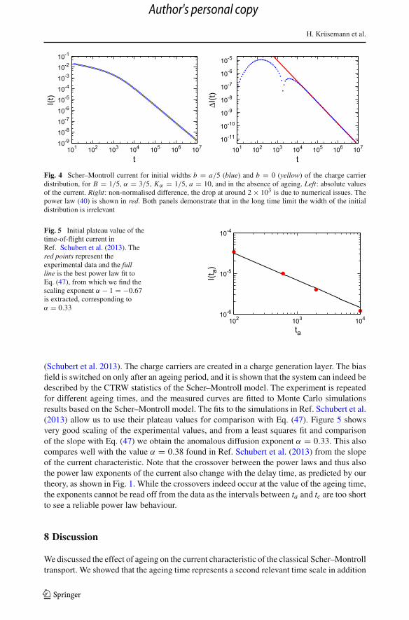
the current produced by an initial δ distribution is only marginal in the long time limit, asshown in Sect. 3. Figure 4 corroborates numerically that both cases lead to almost identicalcurrent characteristic in this long time limit. Since the difference is invisible in this graph,we also show the non-normalised difference on the right of Fig. 4 and find that the behaviouris indeed given by the power law term (40).

7 Experimental Ageing Scher–Montroll Current

The relevance of our calculations from an experimental point of view is shown by the Scher–Montroll current characteristic shown in Fig. 1. In the underlying experiment time-of-flightmeasurements are performed in a dioctyl substituted copolymer PFTBTT (alt-PF8TBTT)

123



10-910-810-710-610-510-410-310-210-1

101 102 103 104 105 106 107

I(t)

t

10-1110-1010-910-810-710-610-5

101 102 103 104 105 106 107

Δ I(t)

t

Fig. 4 Scher–Montroll current for initial widths b = a/5 (blue) and b = 0 (yellow) of the charge carrierdistribution, for B = 1/5, α = 3/5, Kα = 1/5, a = 10, and in the absence of ageing. Left: absolute valuesof the current. Right: non-normalised difference, the drop at around 2 × 103 is due to numerical issues. Thepower law (40) is shown in red. Both panels demonstrate that in the long time limit the width of the initialdistribution is irrelevant

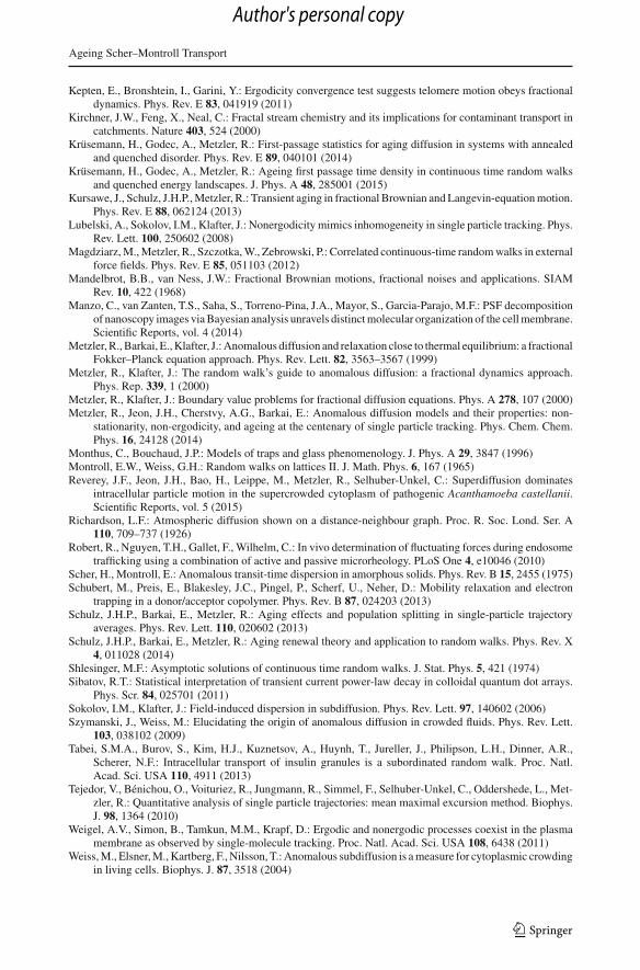
Fig. 5 Initial plateau value of thetime-of-flight current inRef. Schubert et al. (2013). Thered points represent theexperimental data and the fullline is the best power law fit toEq. (47), from which we find thescaling exponent α − 1 = −0.67is extracted, corresponding toα = 0.33

10-6

10-5

10-4

102 103 104

I(ta)

ta

(Schubert et al. 2013). The charge carriers are created in a charge generation layer. The biasfield is switched on only after an ageing period, and it is shown that the system can indeed bedescribed by the CTRW statistics of the Scher–Montroll model. The experiment is repeatedfor different ageing times, and the measured curves are fitted to Monte Carlo simulationsresults based on the Scher–Montroll model. The fits to the simulations in Ref. Schubert et al.(2013) allow us to use their plateau values for comparison with Eq. (47). Figure 5 showsvery good scaling of the experimental values, and from a least squares fit and comparisonof the slope with Eq. (47) we obtain the anomalous diffusion exponent α = 0.33. This alsocompares well with the value α = 0.38 found in Ref. Schubert et al. (2013) from the slopeof the current characteristic. Note that the crossover between the power laws and thus alsothe power law exponents of the current also change with the delay time, as predicted by ourtheory, as shown in Fig. 1. While the crossovers indeed occur at the value of the ageing time,the exponents cannot be read off from the data as the intervals between ta and tc are too shortto see a reliable power law behaviour.

8 Discussion

Wediscussed the effect of ageing on the current characteristic of the classical Scher–Montrolltransport. We showed that the ageing time represents a second relevant time scale in addition

123



to the characteristic crossover time of the non-aged Scher–Montroll transport. Dependingon these time scales an additional intermediate time power law regime and an initial plateaubehaviour of the Scher–Montroll current may emerge. Specifically, for short ageing timesta � tc the current shows the regular Scher–Montroll regimes, following an initial constantregime for t � ta which is relevant only as long as the ageing time ta is not too short. Forlong ageing times ta � ta the three different regimes can be found, separated by the normalcrossover time and the ageing time. If the ageing time is of order of the normal crossovertime, the current crosses over directly to the last regime and the intermediate regime doesnot exist. In the long time limit t � ta all curves show the same power law behaviour. Inparticular, the plateau value connected to the constant velocity of the diffusing charge carriersin this initial regime has a power law dependence on the ageing time. We also demonstratedthat there is no significant effect of a broad initial charge carrier distribution on the long timebehaviour, as expected.We note that the power law regimes found for the first passage densitypreviously (Krüsemann et al. 2014, 2015) are represented in the results derived here, as thefirst passage time contributes to the Scher–Montroll current through the time derivative ofthe survival probability, which enters the equations according to Eq. (23).

Our results may, in principle, be used in experiments to determine the age of an observedScher–Montroll process from the crossover time and the different slopes. In a non-agedprocess the sum of the slopes is exactly −2 whereas in the aged case one finds differentresults, depending on the values of the crossover time tc and the ageing time ta . In turn, if theage is known the dependence of the initial plateau value of the Scher–Montroll current onthe ageing time ta can be used to determine the anomalous scaling exponent of the waitingtime distribution as was shown here using experimental (Schubert et al. 2013). To clearlydistinguish three different regimes in an experiment, the observation time should span aboutnine decades, as the crossovers are no sharp transitions. While this is likely not achievable inmany experimental realisations, by sweeping the parameters it should be possible to exploredifferent windows of the entire first passage distribution and thus observe all occurring powerlaws.

We stress again that while we discussed our results in the language of electrical chargecarriers and currents, this model may equally be used for tracer dispersion in subsurfaceaquifers. Assume that a chemical tracer substance enters the aquifer and then diffuses in theporous environment.As long as there is no significant bias current in the soil, the free diffusionof the tracer corresponds to the ageing period discussed here.After some (ageing) time rainfallcauses the build up of a hydraulic current and drives the tracer towards a catchment. Theresulting current characteristic should display the same crossover behaviours as predictedhere.

Acknowledgments Helpful discussions with Dieter Neher are gratefully acknowledged. RM acknowledgesfinancial support from the Academy of Finland within the Finland Distinguished Professor programme.

References

Akimoto, T., Barkai, E.: Aging generates regular motions in weakly chaotic systems. Phys. Rev. E 87, 032915(2013)

Allegrini, P., Bellazzini, J., Bramanti, G., Ignaccolo,M., Grigolini, P., Yang, J.: Scaling breakdown: a signatureof aging. Phys. Rev. E. 66, 015101 (2002)

Barkai, E.: Fractional Fokker–Planck equation, solution, and application. Phys. Rev. E 63, 046118 (2001)Barkai, E.: Aging in subdiffusion generated by a deterministic dynamical system. Phys. Rev. Lett. 90, 104101

(2003)

123



Barkai, E., Cheng, Y.C.: Aging continuous time random walks. J. Chem. Phys. 118, 6167 (2003)Barkai, E., Garini, Y., Metzler, R.: Strange kinetics of single molecules in living cells. Phys. Today 65, 29

(2012)Bel, G., Barkai, E.:Weak ergodicity breaking in the continuous-time randomwalk. Phys. Rev. Lett. 94, 240602

(2005)Berkowitz, B., Scher, H.: Anomalous transport in random fracture networks. Phys. Rev. Lett. 79, 4038 (1997)Berkowitz,B., Scher,H., Silliman, S.E.:Anomalous transport in laboratory-scale, heterogeneous porousmedia.

Water Resour. Res. 36, 149 (2000)Berkowitz, B., Klafter, J., Metzler, R., Scher, H.: Physical pictures of transport in heterogeneous media:

advection dispersion, random walk, and fractional derivative formulations. Water Resour. Res. 38, 1–9(2002)

Berkowitz, B., Cortis, A., Dentz, M., Scher, H.: Modeling non-Fickian transport in geological formations asa continuous time random walk. Rev. Geophys. 44, RG2003 (2006)

Bodrova, A., Chechkin, A.V., Cherstvy, A.G., Metzler, R.: Quantifying non-ergodic dynamics of force-freegranular gases. Phys. Chem. Chem. Phys. 17, 21791 (2015)

Bouchaud, J.P.: Weak ergodicity breaking and ageing in disordered systems. J. Phys. I (Paris) 2, 1705 (1992)Bouchaud, J.P., Georges, A.: Anomalous diffusion in disordered media: statistical mechanisms, models and

physical applications. Phys. Rep. 195, 12 (1990)Brokmann, X., Hermier, J.P., Messin, G., Desbiolles, P., Bouchaud, J.P., Dahan, M.: Statistical aging and

nonergodicity in the fluorescence of single nanocrystals. Phys. Rev. Lett. 90, 120601 (2003)Burov, S., Metzler, R., Barkai, E.: Aging and nonergodicity beyond the Khinchin theorem. Proc. Natl. Acad.

Sci. USA 107, 13228 (2010)Caspi, A., Granek, R., Elbaum, M.: Enhanced diffusion in active intracellular transport. Phys. Rev. Lett. 85,

5655 (2000)Cherstvy, A.G., Metzler, R.: Population splitting, trapping, and non-ergodicity in heterogeneous diffusion

processes. Phys. Chem. Chem. Phys. 15, 20220 (2013)Cherstvy, A.G., Metzler, R.: Ergodicity breaking and particle spreading in noisy heterogeneous diffusion

processes. J. Chem. Phys. 14, 144105 (2015)Davies, B.: Integral Transforms and Their Applications, vol. 41. Springer Verlag New York Inc, New York

(2002)Di Rienzo, C., Piazza, V., Gratton, E., Beltram, F., Cardarelli, F.: Probing short-range protein Brownian motion

in the cytoplasm of living cells. Nature Commun. 5, 5891 (2014)Donth, E.: The Glass Transition. Springer, Berlin (2001)Edery, Y., Scher, H., Guadagnini, A., Berkowitz, B.: Origins of anomalous transport in heterogeneous media:

structural and dynamic controls. Water Resour. Res. 50, 1490 (2014)Feller, W.: An Introduction to Probability Theory and its Applications, vol. 2. Wiley, New York (1971)Freundlich, H., Krüger, D.: Anomalous diffusion in true solution. Trans. Faraday Soc. 31, 906 (1935)Godrèche, C., Luck, J.M.: Statistics of the occupation time of renewal processes. J. Stat. Phys. 104, 489 (2001)Golding, I., Cox, E.C.: Physical nature of bacterial cytoplasm. Phys. Rev. Lett. 96, 098102 (2006)Goychuk, I.: Viscoelastic subdiffusion: generalised Langevin equation approach. Adv. Chem. Phys. 150, 187

(2012)Habdas, P., Schaar, D., Levitt, A.C., Weeks, E.R.: Forced motion of a probe particle near the colloidal glass

transition. EPL 67, 477 (2004)He, Y., Burov, S., Metzler, R., Barkai, E.: Random time-scale invariant diffusion and transport coefficients.

Phys. Rev. Lett. 101, 058101 (2008)Henkel, M., Pleimling, M., Sanctuary, R. (eds.): Ageing and the Glass Transition. Springer, Berlin (2007)Herzog, R.O., Polotzky, A.: Die Diffusion einiger Farbstoffe. Z. Physik. Chem. 87, 449 (1914)Honigmann, A., Müller, V., Hell, S.W., Eggeling, C.: STED microscopy detects and quantifies liquid phase

separation in lipid membranes using a new far-red emitting fluorescent phosphoglycerolipid analogue.Faraday Disc. 161, 77 (2013)

Jeon, J.H., Tejedor, V., Burov, S., Barkai, E., Selhuber-Unkel, C., Berg-Sørensen, K., Oddershede, L., Metzler,R.: In vivo anomalous diffusion and weak ergodicity breaking of lipid granules. Phys. Rev. Lett. 106,048103 (2011)

Jeon, J.H., Barkai, E., Metzler, R.: Noisy continuous time random walks. J. Chem. Phys. 139, 121916 (2013)Jeon, J.H., Leijnse, N., Oddershede, L., Metzler, R.: Anomalous diffusion and power-law relaxation of the time

averaged mean square displacement in worm-like micellar solutions. New J. Phys. 15, 045011 (2013)Jeon, J.H., Chechkin, A.V., Metzler, R.: Scaled Brownian motion: a paradoxical process with a time dependent

diffusivity for the description of anomalous diffusion. Phys. Chem. Chem. Phys. 16, 15811 (2014)Jung, Y.J., Barkai, E., Silbey, R.J.: Lineshape theory and photon counting statistics for blinking quantum dots:

a Lévy walk process. Chem. Phys. 284, 181 (2002)

123



Kepten, E., Bronshtein, I., Garini, Y.: Ergodicity convergence test suggests telomere motion obeys fractionaldynamics. Phys. Rev. E 83, 041919 (2011)

Kirchner, J.W., Feng, X., Neal, C.: Fractal stream chemistry and its implications for contaminant transport incatchments. Nature 403, 524 (2000)

Krüsemann, H., Godec, A., Metzler, R.: First-passage statistics for aging diffusion in systems with annealedand quenched disorder. Phys. Rev. E 89, 040101 (2014)

Krüsemann, H., Godec, A., Metzler, R.: Ageing first passage time density in continuous time random walksand quenched energy landscapes. J. Phys. A 48, 285001 (2015)

Kursawe, J., Schulz, J.H.P.,Metzler, R.: Transient aging in fractional Brownian and Langevin-equationmotion.Phys. Rev. E 88, 062124 (2013)

Lubelski, A., Sokolov, I.M., Klafter, J.: Nonergodicity mimics inhomogeneity in single particle tracking. Phys.Rev. Lett. 100, 250602 (2008)

Magdziarz,M.,Metzler, R., Szczotka,W., Zebrowski, P.: Correlated continuous-time randomwalks in externalforce fields. Phys. Rev. E 85, 051103 (2012)

Mandelbrot, B.B., van Ness, J.W.: Fractional Brownian motions, fractional noises and applications. SIAMRev. 10, 422 (1968)

Manzo, C., van Zanten, T.S., Saha, S., Torreno-Pina, J.A., Mayor, S., Garcia-Parajo, M.F.: PSF decompositionof nanoscopy images viaBayesian analysis unravels distinctmolecular organization of the cellmembrane.Scientific Reports, vol. 4 (2014)

Metzler,R.,Barkai, E.,Klafter, J.:Anomalous diffusion and relaxation close to thermal equilibrium: a fractionalFokker–Planck equation approach. Phys. Rev. Lett. 82, 3563–3567 (1999)

Metzler, R., Klafter, J.: The random walk’s guide to anomalous diffusion: a fractional dynamics approach.Phys. Rep. 339, 1 (2000)

Metzler, R., Klafter, J.: Boundary value problems for fractional diffusion equations. Phys. A 278, 107 (2000)Metzler, R., Jeon, J.H., Cherstvy, A.G., Barkai, E.: Anomalous diffusion models and their properties: non-

stationarity, non-ergodicity, and ageing at the centenary of single particle tracking. Phys. Chem. Chem.Phys. 16, 24128 (2014)

Monthus, C., Bouchaud, J.P.: Models of traps and glass phenomenology. J. Phys. A 29, 3847 (1996)Montroll, E.W., Weiss, G.H.: Random walks on lattices II. J. Math. Phys. 6, 167 (1965)Reverey, J.F., Jeon, J.H., Bao, H., Leippe, M., Metzler, R., Selhuber-Unkel, C.: Superdiffusion dominates

intracellular particle motion in the supercrowded cytoplasm of pathogenic Acanthamoeba castellanii.Scientific Reports, vol. 5 (2015)

Richardson, L.F.: Atmospheric diffusion shown on a distance-neighbour graph. Proc. R. Soc. Lond. Ser. A110, 709–737 (1926)

Robert, R., Nguyen, T.H., Gallet, F., Wilhelm, C.: In vivo determination of fluctuating forces during endosometrafficking using a combination of active and passive microrheology. PLoS One 4, e10046 (2010)

Scher, H., Montroll, E.: Anomalous transit-time dispersion in amorphous solids. Phys. Rev. B 15, 2455 (1975)Schubert, M., Preis, E., Blakesley, J.C., Pingel, P., Scherf, U., Neher, D.: Mobility relaxation and electron

trapping in a donor/acceptor copolymer. Phys. Rev. B 87, 024203 (2013)Schulz, J.H.P., Barkai, E., Metzler, R.: Aging effects and population splitting in single-particle trajectory

averages. Phys. Rev. Lett. 110, 020602 (2013)Schulz, J.H.P., Barkai, E., Metzler, R.: Aging renewal theory and application to random walks. Phys. Rev. X

4, 011028 (2014)Shlesinger, M.F.: Asymptotic solutions of continuous time random walks. J. Stat. Phys. 5, 421 (1974)Sibatov, R.T.: Statistical interpretation of transient current power-law decay in colloidal quantum dot arrays.

Phys. Scr. 84, 025701 (2011)Sokolov, I.M., Klafter, J.: Field-induced dispersion in subdiffusion. Phys. Rev. Lett. 97, 140602 (2006)Szymanski, J., Weiss, M.: Elucidating the origin of anomalous diffusion in crowded fluids. Phys. Rev. Lett.

103, 038102 (2009)Tabei, S.M.A., Burov, S., Kim, H.J., Kuznetsov, A., Huynh, T., Jureller, J., Philipson, L.H., Dinner, A.R.,

Scherer, N.F.: Intracellular transport of insulin granules is a subordinated random walk. Proc. Natl.Acad. Sci. USA 110, 4911 (2013)

Tejedor, V., Bénichou, O., Voituriez, R., Jungmann, R., Simmel, F., Selhuber-Unkel, C., Oddershede, L., Met-zler, R.: Quantitative analysis of single particle trajectories: mean maximal excursion method. Biophys.J. 98, 1364 (2010)

Weigel, A.V., Simon, B., Tamkun, M.M., Krapf, D.: Ergodic and nonergodic processes coexist in the plasmamembrane as observed by single-molecule tracking. Proc. Natl. Acad. Sci. USA 108, 6438 (2011)

Weiss,M., Elsner,M.,Kartberg, F., Nilsson, T.:Anomalous subdiffusion is ameasure for cytoplasmic crowdingin living cells. Biophys. J. 87, 3518 (2004)

123



Wolfram, S.: Mathematica: A System for Doing Mathematics by Computer. Addison Wesley Longman Pub-lishing Co., Inc., Boston (1991)

Wong, I.Y., Gardel, M.L., Reichman, D.R., Weeks, E.R., Valentine, M.T., Bausch, A.R., Weitz, D.A.: Anom-alous diffusion probes microstructure dynamics of entangled F-actin networks. Phys. Rev. Lett. 92,178101 (2004)

Xu, Q., Feng, L., Sha, R., Seemann, N.C., Chaikin, P.M.: Subdiffusion of a sticky particle on a surface. Phys.Rev. Lett. 106, 228102 (2011)

123


ageing scher–montroll transport - uni-potsdam.demetz/papers/2016_krueschwarme_tipm1… · ageing...

Documents