After Midnight: A Regression Discontinuity

Design in Length of Postpartum Hospital Stays∗

Douglas Almond† and Joseph J. Doyle Jr.‡

February 21, 2008

Abstract

Patients who receive more hospital treatment tend to have worse un-derlying health, confounding estimates of the returns to such care. Thispaper compares the costs and benefits of extending the length of hospitalstay following delivery using a discontinuity in stay length for infants bornclose to midnight. Third-party reimbursement rules in California entitlenewborns to a minimum number of hospital “days,” counted as the num-ber of midnights in care. A newborn delivered at 12:05 a.m. will havean extra night of reimbursable care compared to an infant born minutesearlier. We use a dataset of all California births from 1991-2002, includ-ing nearly 100,000 births within 20 minutes of midnight, and find thatchildren born just prior to midnight have significantly shorter lengths ofstay than those born just after midnight, despite similar observable char-acteristics. Furthermore, a law change in 1997 entitled newborns to aminimum of 2 days in care. The midnight discontinuity can thereforebe used to consider two distinct treatments: increasing stay length fromone to two nights (prior to the law change) and from two to three nights(following the law change). On both margins, we find no effect of staylength on readmissions or mortality for either the infant or the mother,and the estimates are precise. The results suggest that for uncomplicatedbirths, longer hospitals stays incur substantial costs without apparenthealth benefits.

∗Josh Angrist, Janet Currie, Randall Ellis, Michael Greenstone, Rick Hornbeck, DougMiller, Roberto Rigobon, Jon Skinner, Tom Stoker, and Tavneet Suri provided helpful com-ments and discussions. We also thank Jan Morgan of the California Healthcare InformationResource Center for helpful advice and discussions and Sammy Burfeind, whose birth inspiredour empirical approach.

†Columbia University and NBER: da2152@columbia.edu‡MIT and NBER: jjdoyle@mit.edu

1

1 Introduction

The amount of time spent in hospital after childbirth has changed substantiallyover the last generation. Between 1970 and 1995, the average length of stay fellfrom 4.1 to 2.1 days (Figure 1). Increased cesarean deliveries over this sameperiod masks even larger decreases in stay length conditional on method ofdelivery [9]. By the early 1990s, third-party payers routinely declined coverageof hospital stays longer than 24 hours for uncomplicated vaginal deliveries [1].

The shift toward shorter postpartum stays was controversial and politicallyunpopular. Between 1995 and 1998, 42 states passed laws requiring insurers tocover minimum postpartum lengths of stay [11]. In January 1998, the federalgovernment followed suit, mandating a minimum stay of 2 days. The averagelength of hospital stay for mothers increased 20% between 1995 and 1998, andnewborns’ stays increased from 2.8 days to 3.2 [20]. The fraction of vaginaldeliveries with stay lengths under two days fell by half – from 47% in 1995 to23% in 1998 (Figure 2).

As delivery is one of the most commonly performed surgical procedure inthe U.S., secular changes in stay length have significant implications for healthcare costs and health outcomes.1 Studies of the law changes themselves, how-ever, have yielded mixed evidence. For example, Evans et al. [11] found thatCalifornia’s law improved health outcomes for vaginal deliveries in the Medicaidpopulation, but not for privately-insured patients. Implementation of the lawwas not immediate, and time-series comparisons yield unbiased estimates of thehealth impact to the extent that other health determinants did not happen tochange over the implementation period.

Our approach departs from previous work by comparing infants born atnearly the same point in time. We use the fact that billing rules reimbursehospitals based on the number of days the newborn is in the hospital. Thesedays are counted as the number of midnights in care. A newborn delivered at12:05 am will have nearly a full day in care before being “logged” as presentin the hospital, whereas a newborn delivered at 11:55 p.m. will be counted aspresent only 5 minutes after delivery. As a result, those born just after midnighthave an extra night of reimbursable care compared to those born just prior tomidnight.

The analysis uses a unique data set of hospital discharge data linked to birthand death certificates for all births in California from 1991 to 2002. These datareport the hour and minute of birth. An additional dimension of our empiricalanalysis is made possible by the 1997 Newborns’ and Mothers’ Health Act: alaw in California that mandates insurance coverage for a minimum of 2 days inhospital. This allows us to trace out the effect of an increase in stay lengthusing the midnight discontinuity from two different baselines. Prior to the law,the midnight threshold primarily induced variation between 0 and 1 additionalmidnights (i.e. one versus two total nights in the hospital). Following the law,

1Delivery is the most commonly performed surgical procedure in our analysis period. Since2002, operations involving the cardiovascular system have been more frequently performedthan obstetrical procedures (NCHS [20] and various additional years).

2

the midnight threshold primarily induced patients to switch between 1 and 2additional midnights (or two versus three total nights in hospital). Thus, we canuse the midnight rule to evaluate the effect of a two-day minimum stay dictatedby law (and recommended by the American Academy of Pediatrics) comparedto a further expansion in length of stay from two to three nights.

We find that the difference in privately-born costs associated with the minuteof birth generates a substantial difference in average stay length, despite nearlyidentical observable characteristics. Infants born shortly after midnight spendan additional 0.25 nights in the hospital – a difference similar to the change inlength of stay when the California mandate increased the minimum stay by oneday.

Despite the longer stays for infants born after midnight, we find no effect ofa post-midnight birth on health outcomes. Both visual inspections of the rawdata and models that control for patient characteristics reveal estimates close tozero for hospital readmissions and infant mortality. Given that these follow-upexpenses were covered by insurance companies, the push toward shorter lengthsof stay in the early 1990s presumably reduced costs for insurers.

The results apply to a population that is induced to have a longer hospitalstay as a result of a post-midnight birth. A prior, these are likely uncomplicatedcases where the minute of birth is plausibly exogenous and the stays are not ex-pected to be especially long – patients in a part of the health distribution wherethe minimum stay legislation may be most likely to bind. While these “compli-ers” cannot be identified in the data, we do estimate the mean characteristics ofthis population, and, indeed, they are less likely to be low birthweight and morelikely to be full term compared to the full population. Furthermore, largereffects of a post-midnight birth on length of stay are found for those more likelyto have benefitted from it – particularly prior to the 1997 law, when average staylengths were shorter. Among mothers covered by Medicaid, for example, theincrease in stay length for births after midnight was approximately 40% longerthan the post-midnight increase among non-Medicaid births. Nevertheless, nohealth outcome differences were detected within this population.

The rest of the paper is organized as follows. Section 2 considers the back-ground that led to early discharge laws and the role that minute of birth playsin determining the length of stay. Section 3 describes the data. Section 4describes the model and estimation, describing the manner in which we traceout the effects of length of stay from 0 to 1 and from 1 to 2 additional nightsin care. Section 5 presents the results and section 6 interprets the results incomparison to the costs of an additional night in care. Section 7 concludes.

2 Background

Between 1970 and 1995, the average length of stay for a vaginal delivery fell from3.9 to 1.7 days (Figure 1). For cesarean births, the corresponding numbers are7.8 to 3.6 days [9]. In the mid-1990s, this decrease was halted, and if anything

3

slight increases in average stays followed.2 For short-stays, the pattern is morestark. Figure 2 plots the share of vaginal births with stays under 2 days from1970-2004. There is a doubling of these “early discharges” from 1990 to 1995,followed by a sharp and sustained reduction.

The practice of “drive-through delivery” formed a rallying point against cost-saving measures imposed by third-party payers [13]. In 1995, the official journalof the American Academy of Pediatrics ran a commentary entitled: “Early dis-charge, in the end: maternal abuse, child neglect, and physician harassment,”3

that warned inadequate screening of newborns was the “most dangerous andpotentially long-term effect of early discharge.” In particular, early dischargehad caused the “re-emergence” of jaundice as a cause of hospital re-admission[6]. In 2005, the American Academy of Pediatrics published criteria for thedischarge of newborns, noting it is“unlikely that fulfillment of these criteria andconditions can be accomplished in 48 hours” even for healthy newborns [1].

On August 26, 1997 the California Newborns’ and Mothers’ Health Act cameinto effect in California that entitled newborns to 48 hours of inpatient care, aswell as coverage for early follow-up care if the newborn is discharged early. Afederal law would come into existence the following year. Figure 3 shows thatthe fraction of vaginal births in California that had an early discharge increasedto 75% prior to the law change, and decreased from October 1997 to February1998 to 50%.4

2.1 Minimum Length of Stay Laws

Previous work comparing newborns born just before and after such law changeshave consistently found that the laws increased stay lengths. Findings for healthimpacts, however, have been mixed.

Meara et al. [18] studied newborns covered by the Medicaid program in Ohiofrom 1991-1998. Using an interrupted time-series design, they found “modestreductions” in readmissions for jaundice and emergency department visits fol-lowing the introduction of minimum-stay legislation in 1996. All-cause rehospi-talization, as well as readmissions for dehydration and infection, were not foundto be affected by the law change.

Madden et al. [15] analyzed newborn health outcomes in a MassachusettsHMO before and after implementation of the state’s early discharge law inFebruary 1996. They found longer stay lengths, but no effects on emergencydepartment visits or re-hospitalizations. However, at the end of 1994 the HMOinitiated a program for deliveries that included “increased prenatal participa-tion” and a home visit by a nurse within 48 hours of discharge[15]. This programwas discontinued when the state discharge law came in to effect.

Evans et al. [11] also use a time-series design to analyze the impact of Califor-nia’s minimum stay law, passed and enacted in August 1997. The law mandated

2NCHS [20] and various additional years.3As noted by Hyman [13].4The spikes seen represent December 24 each year when short stays are particularly com-

mon.

4

that insurance cover at least two days in the hospital or an early follow-up visitin a physician’s office or at home. Between August 1997 and January of 1998,when the federal early-discharge law came in to effect, the fraction of newbornsdischarged “early” fell sharply (Figure 3). Like Meara et al. [18], Evans et al.[11] find decreases in readmission rates for the Medicaid population with vagi-nal deliveries. Evans et al. [11] also find some improvements in outcomes forprivately-insured vaginal births that exhibited some complications following theearly discharge law.

Several recent papers have emphasized the persistence of health complica-tions related to early discharge despite implementation of laws mandating cov-erage of minimum hospital stays. Noting that early discharge is not precludedunder the federal early discharge law, Galbraith et al. [12] found that 49.4% oftheir sample of California births in 1999 were discharged “early”, i.e. prior tothe expiration of insurance coverage.5 Deliveries paid for by Medicaid or wherethe mother was Hispanic were more likely to be discharged early. Galbraithet al. [12] concluded that: “issuance of professional guidelines and legislationalone cannot ensure adequate postnatal services, particularly among the groupsof socioeconomically vulnerable newborns.” Similarly, Paul et al. [21] arguedthat “well-intentioned [early discharge] legislation and current practice may notbe sufficiently protecting the health of newborns.”

In an attempt to buffer the presumed effects of early discharge that occurreddespite the legislation, early follow-up visits were mandated in these cases. Pre-vious evidence suggests that such a mandate is unlikely to affect the take up ofsuch services, however. Meara et al. [18] find no effect of Ohio minimum stay-early follow-up visit legislation on the take up of early follow-up care amongthe state’s Medicaid population, and Galbraith et al. [12] find no difference inearly follow-up care for newborns who were discharged early versus those whowere not. These results suggest that our comparisons of effects before and theCalifornia law are unlikely to be affected by differences in early follow-up care.

The identifying assumption underlying the interrupted time-series approachis that the trend in length of stay and outcomes prior to the law change describesthe counterfactual length of stay and outcomes after the law change. If otherinterventions happened at the same time as the law change, then the before-aftereffects may reflect both the law change and the complementary interventions.For example, if the policy change was accompanied by warnings of the increasein jaundice in the early 1990s, then policies that aimed to reduce jaundiceinfections may have happened at the same time as the extended stays. Ifhospitals began responding to public criticism prior to the enactment, or if thelaw imposed short-run costs on hospitals, then the change in outcomes beforeand after the law will measure the effect of the change in length of stay as wellas the response to the law.6

5And as defined by the American College of Obstetricians: under 48 hours for vaginaldeliveries and under 96 ours for cesarian births [12].

6Our analysis of California data finds that the daily number of newborns in the hospitalincreased by approximately 10% between June 1997 and August 1998 in California. Treatmentchoices do not appear to change at the time of the law, although there is suggestive evidence

5

2.2 Time of Birth and Stay Length

Length of stay is typically measured as the number of midnights spent in hos-pital. For postpartum stays, care is generally reimbursed for a predeterminednumber of midnights in care, with longer stays requiring physician approval.For example, the Medicaid program in California, known as “Medi-Cal”, issuesthe following guidelines regarding prior authorization for obstetric admissions:

Welfare and Institutions Code, Section 14132.42, mandates thata minimum of 48 hours of inpatient hospital care following a normalvaginal delivery and 96 hours following a delivery by cesarean sec-tion are reimbursable without prior authorization. For [TreatmentAuthorization Requests (TARs)] and claims processing purposes, itis necessary to use calendar days instead of hours to implement theserequirements. Therefore, a maximum of two consecutive days follow-ing a vaginal delivery or four consecutive days following a deliveryby cesarean section is reimbursable, without a Treatment Authoriza-tion Request. The post-delivery TAR-free period begins at midnightafter the mother delivers. [19]

For a birth occurring at 11:59p.m., the number of reimbursable days in carebegins one minute later, whereas births just after midnight are afforded nearlya full 24-hour period before the number of reimbursable days in care begin tobe counted.

An underlying assumption is that for uncomplicated deliveries, the actualminute of birth around midnight is effectively random. There are ways ofincreasing or decreasing the speed of the delivery, however, and physician mayhave some discretion over the recording of the time of the delivery. In termsof incentives, the patient and the insurer would prefer a post-midnight birth,as billing for time in the hospital would not begin until one day later. Thehospital would likely prefer a pre-midnight birth to begin billing for the timein care sooner. The cost to the hospital of supervising the child would alsodecline if the birth occurred before midnight and the discharge time was sooner.To the extent that the physician’s interest is aligned with the patient (or theinsurer), there may be a tendency to record births after midnight, whereas ifthe incentives are aligned with the hospital, the tendency would be to recordbirths just before midnight. We will consider the frequency of births aroundmidnight for all births, as well as births that occur in Kaiser Hospitals–hospitalswhere the insurer owns the hospital.

If the birth occurs after midnight, the family effectively has a property rightto the hospital bed for one additional night. In a setting of costless bargaining,this increase in the property right might not be expected to have any impacton stay length [8]. If the insurer wanted to bargain for shorter stay lengths,however, they would face political costs. Before the minimum stay law, policy

that cesarean section rates increased beginning in January 1998; they were close to 21% for 3years prior to the federal mandate, increased to 22% in March 1998, and continued to increaseto 27% by the end of the sample period (2002).

6

and practice entitled newborns to only 1 day in the hospital. After the lawchange, insurers are limited to the use the early follow-up care as an incentivefor an early discharge, although previous evidence suggests that early follow-upvisits are not determined by length of stay.

Previous work most closely related to our approach is Malkin et al. [16].They used 4-hour categories in the time of birth as an instrument for lengthof stay. They found significant reductions in newborn readmissions with longerpostpartum hospital stays. However, births scheduled for “business hours” mayhave different baseline characteristics compared to births later in the day (re-flecting, e.g., the scheduling of high-risk deliveries). Indeed, in California, wefind that baseline health and demographic characteristics are on average dif-ferent during “business hours” compared to the overnight hours.7 For thisreason, we will restrict comparisons to births just before and after midnightwhen observable characteristics are similar across the newborns.

3 Data

3.1 Description

Our data include the universe of live births in California from 1991-2002, some6.6 million records. We focus on the 270,000 births occurring between 11 p.m.and 1 a.m. The California Office of Statewide Health Planning and Developmentcreated a research database that includes hospital discharge records linked tobirth and death certificate records. For a given birth, discharge data are avail-able nine months prior to delivery so as to capture the course of antepartum andinpatient care. In addition, hospital admissions up to one year after deliveryare matched to the birth record. Death certificate data provide a measure ofmortality, while the birth certificate includes a wealth of information about theparents and the circumstances of the birth itself.

The hospital discharge data include the patient’s age, procedure and diag-nosis codes, primary payer, day of the week, hospital ownership information,and admission and discharge date. Beginning in 1995, whether the birth wasscheduled or unscheduled is reported as well.

Length of stay is reported in the data as the discharge date minus the ad-mission date: the total number of midnights in care. The admission date isthe date of birth for the newborn.8 The main measure of resource usage in

7As in Malkin (2000) we find infants born between 8am and 12 noon have a length of staythat is 7 hours longer than those born between 8pm and 12 midnight (discharge time wasassumed to be 5pm for those with same day discharges and 1pm for those who stay at leastone night in the hospital). We also find statistically significant decreases in readmissionswith an increase in length of stay using these 4-hour blocks as instruments. The groups differsubstantially, however, with the largest differences found for mother’s first birth (34% formorning births vs. 44% for 8-midnight births), induced labor (only 6% for 8am to noon vs.12% for those occurring later in the evening), and cesarean section (30% vs. 14% for thoseborn between 8am and noon vs. midnight to 4am).

8Despite the potential incentive on behalf of the patient or the insurer to record the ad-mission date as after midnight, this does not appear to occur.

7

the analysis will be the number of additional midnights in care: the number ofmidnights in the hospital not counting the initial one that defines the threshold.That is, our measure for those born after midnight is the usual one; for thoseborn before midnight, we subtract one from the usual length of stay so as toremove the mechanical midnight that is not related to the true length of stayin the hospital.9

The linked birth certificate data report pregnancy and birth characteristicsthat are not available in hospital discharge data. The pregnancy is described bythe number of prenatal visits, as well as the presence of any complications, suchas hypertension or diabetes. The use of ultrasound and amniocentesis is alsorecorded. Parents are described by their age and educational attainment, aswell as the mother’s birthplace. For the newborn, birth weight and gestationalage (in days) are reported. When gestational age is used as a control, it ismeasured as the number of days not including the midnight that defines thethreshold. While Race/Ethnicity of the newborn will be considered, Hispanicbirths were no longer separately identified in our data after 1995. We observebirth complications, including measures of the use of interventions, whether thelabor was stimulated, and whether the labor was induced. The mother’s day ofadmission and the precise time of birth, essential to implementing our design,are recorded. Discharge time is not recorded, so our length of stay measure is indays. While we would prefer a more detailed measurement of stay length, in thespirit of “not biting the hand that feeds,” we note that its absence is presumablywhat makes our discontinuity design possible. Finally, it is possible that infantsborn prior to midnight may stay later on the day of discharge compared tonewborns who stay an additional night in the hospital due to the post-midnightbirth. As such, the results below consider the effect of having an extra night inthe hospital.

3.2 Analysis Sample

The main analysis will consider vaginal births within 20 minutes of midnight;births by cesarean section will be considered separately. Newborns with lengthsof stay of more than 28 days (5.2%) are excluded. These outliers are less likelyto be affected by the accounting rules and may skew the mean differences beforeand after midnight. To focus on patients where the births are most likely to haverandom variation with regard to the timing of the birth, unscheduled births areconsidered after 1995, which excludes 15% of the remaining births. Scheduledbirths will be considered separately as well. 1% of births were excluded becausedelivery took place outside of a hospital. Another 4% of the data have missingcovariate information; results will be shown with and without these births.10

9Total hospital charges are available in the data, but those born just before midnight arebilled for a night in care almost immediately and have slightly higher accounting chargesdespite spending less time in the hospital.

10In the pooled sample over all of the years, post-midnight births are less likely to resultfrom a c-section (17.5% vs.18.8%) and less likely to have stays of 28 or more days (4.6% vs.6.1%). Differences in home births, scheduled births, and missing covariates are small and not

8

Figures of raw means by minute of birth and local linear regressions willbe shown using data for every minute of the day. Models are also estimatedwith two samples: a 40-minute sample and a 2-hour sample, which include datawithin those windows around midnight. Due to the potential of measurementerror (e.g. a spike in births on the hour typically identify births that occurred atany time during that hour or attempts to influence the reported length of stay ofthose born close to midnight by recording a time of before or after midnight) themain analysis excludes the births from 11:56 p.m. to 12:04 a.m. The 40-minutesample, then, includes births fewer than 20 minutes from 11:55 p.m. or 12:05a.m.11

The final cut of the data considers infants born before and after the lawchange in California. The law came into effect on August 26, 1997. Births fromJanuary 1, 1991 to July 31, 1997 will be used to estimate the models before thelaw change, and births from September 1, 1997 to December 31, 2002 will beconsidered for post-law-change births. The resulting 40-minute samples includenearly 60,000 observations prior to the law change and over 30,000 observationsafter the law change.

4 Model and Estimation

We compare birth outcomes on either side of the midnight threshold. The effectof an extra night in the hospital on these outcomes we estimate is the ratio ofthe outcome difference and the length of stay difference. This estimate measuresthe local average treatment effect (LATE) for those infants who receive an extranight in the hospital as a result of being born after midnight [4]. Specifically, weare estimating effects for those who stay an extra night at the hospital becausethe infant is entitled to an extra day without charge due to the time of birtharound midnight. Presumably, those induced to stay longer are not a randomdraw from the population. In particular, infants born around midnight likelydiffer from those planned to be born earlier in the day. For this reason, a prioriour estimates may be expected to differ from those previously estimated usingthe minimum stay-length mandates. Further, infants induced to stay an extranight as a result of the time of birth around midnight exclude families who wishto leave the hospital soon after birth or newborns with serious health compli-cations who will stay in the hospital much longer than two nights regardless(these groups are also excluded from the time-series estimates that consider thelaw changes.)

Our exposition of the potential outcomes framework (Section 4.1), conditionsfor LATE estimation (Section 4.2), and multi-valued treatment (Section 4.3)follows Angrist & Imbens [3] and their example of estimating returns to schoolingusing the quarter of birth instrument closely.

statististically significant across the groups.11The sample mimics the nonparametric estimates that include births less than 20 minutes

from the threshold. With the threshold at minute t = 0, this includes births from -19 ≤ t ≤19. These times are 11:37 p.m. to 11:55 p.m. and 12:05 a.m. to 12:24 a.m.

9

4.1 Potential Outcomes Framework

First, we define the binary variable Z:

Z ={

0 born just before midnight1 born just after midnight

We are interested in the (multi-valued) treatment variable L, reflecting thelength of hospital stay. For infants born close to midnight, we consider thenumber of additional midnights in care. Specifically, we define L as:

L =

0 no additional midnights1 one additional midnight2 two additional midnightsJ three or more additional midnights

LZ is the number of additional midnights conditional on whether the infantwas born just prior to midnight (Z = 0) or just after midnight (Z = 1). New-borns are observed being born either before or after midnight, however, andwhat we actually observe is:

L = LZ = Z · L1 + (1− Z) · L0 (1)

Further, we assume a set of potential health outcomes Yj (e.g. whether anewborn is re-admitted to a hospital in first 28 days of life) exists for eachnewborn for each of the possible durations of initial hospital stay j = 0 to J .

4.2 Conditions required for estimating LATE

Three conditions must be met in order to interpret our estimate as a localaverage treatment effect. Again, this section follows Angrist & Imbens [3].

1. There is a first stage.

Pr(L1 ≥ j > L0) > 0 for some j.

The probability of an additional midnight is higher for those born just aftermidnight for some length of stay j. We explore this condition empirically.

2. MonotonicityL1 − L0 ≥ 0

for each newborn with probability 1.12 Anyone in the population whowould stay an additional midnight were she born before midnight (a staythat would require physician approval for reimbursement) would also staythat additional midnight if she were born after midnight (when it is auto-matically reimbursed). This assumption is not verifiable because we only

12Alternatively, L1 − L0 ≤ 0 for each newborn would also satisfy monotonicity, but is notplausible in this context.

10

observe L0 or L1. Monotonicity would seem quite plausible in our appli-cation as those who were born before midnight and stayed an additionalmidnight in any event would receive a “free” night by being born aftermidnight. This condition serves to prohibit “defiers” (i.e. newborns whoviolate the monotonicity assumption by receiving extra time in the hospi-tal due to being born earlier).13 Angrist & Imbens [3] demonstrate thatmonotonicity has the testable implication that the c.d.f. of L for thoseborn just before and just after midnight should not cross. That our datasatisfy this implication is demonstrated in the results below.

3. Independence

(L0, L1, Y0, Y1, Y2, YJ) are jointly independent of Z.

The independence assumption is satisfied if the time of birth around mid-night exhibits random variation. While not testable, we will consider thefrequency of birth before and after midnight, as well as observable char-acteristics to consider whether those born after midnight appear differentfrom those born before midnight.

4.3 Multi-Valued Treatment

Under the conditions above, the local average treatment effect is the ratio ofthe outcome difference to the length of stay difference. As j ranges from 0 toJ , the effect for increases in the number of nights from one to two; from two tothree; and so on are averaged together to yield the “average causal response”[3].14 The weight attached to each increment in stay length is given by:

$j =Pr(L1 ≥ j > L0)

J∑i

Pr(L1 ≥ i > L0)

which is proportional to:

Pr(L ≥ j | Z = 1)− Pr(L ≥ j | Z = 0)

Passage of California Newborns’ and Mothers’ Act in 1997 changed theweights used to calculate the average causal response dramatically. Prior to

13There could be a mechanical effect of a pre-midnight birth having a longer length of stayfor a fixed discharge time, where an 11:30pm birth would have an extra hour in care comparedto one born at 12:30am. This is one reason considering births just before and after midnightis important.

14If a post-midnight birth induced an infant to stay two extra nights, then effects from suchincreases would be included in the weighted average as well. This might be possible if an extranight in the hospital leads to the detection of a problem that results in even longer lengths ofstay. For the most part, however, the inducement is created by the entitlement to one morenight and we consider the one-unit increases in lenght of stay as a result.

11

the law change, the midnight threshold increased the number of additional mid-nights primarily from zero to one (or one to two total ”nights” in the hospital).After the law change, stay length increased from one to two additional mid-nights due to the midnight rule (see Section 5.1.2 for details). By estimatingresults separately for births before and after the law change, the potential fordiminishing returns to length of stay can be examined.

4.4 Description of Compliers

The local average treatment effect is the average treatment effect for ”com-pliers”: those who are induced to have a longer stay as a result of the post-midnight birth. In contrast, “always takers” or “never takers” have stay lengthsthat are unaffected by the minute of birth. It is not possible to identify thecompliers, but it is possible to describe their average observable characteristics,E(X|D1 = 1, D0 = 0).15

For example, define the binary variable D: to be an indicator for a long stay(e.g. more than 1 night prior to the law change and more than 2 nights afterthe law change):

D ={

0 short stay1 long stay

Also define DZ as the value D would take if Z were either 0 or 1. Z is againassumed to be independent of D. Compliers in this context are such thatD1 = 1 and D0 = 0 .

For example, E(X|D1 = 1) = E(X|D = 1, Z = 1) represents the char-acteristics of those with long stays who are born after midnight and can beestimated by sample means. This can be written as a weighted average of thecharacteristics of always takers and compliers:

E(X|D1 = 1) = E(X|D1 = 1, D0 = 1)P (D0 = 1|D1 = 1)+E(X|D1 = 1, D0 = 0)P (D0 = 0|D1 = 1) (2)

Always takers can be described by the characteristics of individuals whoare born before midnight (Z = 0) yet have longer stays (D = 1). That is,the E(X|D1 = 1, D0 = 1) = E(X|D0 = 1), by the monotonicity condition(D1 − D0 ≥ 0). The last term is E(X|D = 1, Z = 0), which can also beestimated by sample means.

For the probability terms:

15Abadie [2] showed that characterisitics of compliers can be described using his kappaweighting scheme. It is also known that for binary characteristics and a binary instrument,the relative likelihood that an individual in a particular group is a complier is the ratio of thefirst-stage coefficient on the instrument estimated on that group’s subsample to the first-stagecoefficient for the full sample.

12

P (D0 = 1) = P (D0 = 1|D1 = 1)P (D1 = 1) + P (D0 = 1|D1 = 0)P (D1 = 0)= P (D0 = 1|D1 = 1)P (D1 = 1) by the monotonicity condition.

P (D0 = 1) and P (D1 = 1) can be estimated as the sample proportion ofthose born before midnight with long stays and the proportion of those bornafter midnight with long stays, respectively. The first is an estimate of thepopulation proportion of always takers πA, by the independence of Z. Similarly,for those born after midnight, those with short stays can be used to estimate thepopulation fraction who are never takers, πN . The proportion of the populationwho are compliers is then πC = 1− πA − πN , as “defiers” are assumed away bythe monotonicity condition. Among the group born after midnight, the fractionwith longer stays, P (D1 = 1), is πC + πA. Meanwhile, P (D0 = 1|D1 = 1) =πA/(πA + πC), and P (D0 = 0|D1 = 1) = πC/(πA + πC).

(2) can then be re-arranged, and the expected characteristics of the complierscan be written as:

E(X|D1 = 1, D0 = 0) =πC + πA

πC

[E(X|D1 = 1)− πA

πC + πAE(X|D1 = 1, D0 = 1)

]

=πC + πA

πC

[E(X|D = 1, Z = 1)− πA

πC + πAE(X|D = 1, Z = 0)

]

Each of these terms can be estimated in the sample.

4.5 Estimation

We begin by examining the first stage – the relationship between the time ofbirth and the length of stay – and then proceed to the reduced form – therelationship between the time of birth and the health outcomes. Local lin-ear regressions before and after are estimated using a triangle kernel [17][7].Asymptotic standard errors are also reported [22].

In addition, we estimate parametric models that include covariates and lin-ear trends that vary before and after midnight. This is a simple local linearestimator with a rectangle kernel and where the weights do not decay as thedistance from midnight increases [14]. For outcomes Y (including length of stay,readmissions, and mortality), the models for infant i born at minute t from amidnight (t=0) cutoff are as follows:

Yit = β0 + β11(t ≥ 0) + β21(t ≥ 0) ∗ t + β31(t < 0) ∗ t + β4Xi + εit (3)

where X is a vector of observable birth characteristics.16

16In practice, the analysis samples exclude births within 10 minutes of midnight. t=-1 justprior to the cutoff (11:55pm) and t=0 at the cutoff (12:05am).

13

This basic regression discontinuity model is estimated using Ordinary LeastSquares for length of stay. Additional tests of robustness with regard to theestimation are also reported. For the binary outcomes of readmissions andmortality, probit models are estimated and marginal effects at the mean of thecontrol variables are reported. Heteroskedasticity-robust standard errors arereported for these models.

4.5.1 Choice of Bandwidth

Across the outcomes, bandwidths of close to 10 minutes were found to minimizethe sum of squared errors between the local linear estimator and a fourth-degreepolynomial model estimated within two hours of midnight. Local estimationat a boundary is generally thought to require a somewhat larger bandwidthcompared to interior points, and we applied a rule of thumb used in densityestimation at a boundary of two times the cross-validation bandwidth [26], ora twenty-minute pilot bandwidth in this case. Shorter and longer bandwidthsare considered as well. Relatively wider bandwidths appear appropriate giventhat we find a sustained increase in length of stay following midnight, and ifthis length of stay affects outcomes, a shift in the readmission or mortality rateshould be sustained through the first hour as well. The tradeoff is that infantsborn far from midnight are more likely to differ from one another. We do notexpect infants born at 11:00 p.m. to be so very different from those born at 1:00a.m.

5 Results

5.1 Unconditional Estimates

5.1.1 Frequency of Births Around Midnight

Do physicians systematically misreport time of birth around the midnight thresh-old? As noted above, physicians may have an incentive to record births as oc-curring earlier or later than midnight. Figure 4 provides a visual check on thisbehavior, plotting the number of births by minute of the day [17]. Births aremore frequent during “business hours” of 7:00 a.m. to 5:00 p.m. The frequencydeclines until midnight and remains fairly stable until around 7:00 a.m. Thetime of birth is more likely to be reported on the even hour and additionally attimes ending in 0 or 5, due to rounding.

Much of the analysis will focus on births between 11 p.m. and 1 a.m. andFigure 4B shows roughly 2500 births are recorded each minute, while 3000births are found at the 5 minute marks. The largest spikes occur at 11:00p.m. and 12:01 a.m. 12:00 midnight–the only time that uses the number 24 asthe hour–has fewer observations (N=734), possibly due to physicians makingclear that the birth occurred the following day. The spike at 12:01 is similar tothe spike at 11:00p.m., though it is slightly larger than the spike at 1:00 a.m.

14

These spikes likely reflect births that occurred at any time during that hour–one reason to exclude births at 12:01 a.m. as most of these births occurredlater in the hour. Other than births reported to occur at 2400 (midnight), thenumber of observations is similar in the hour before and after midnight. 153,180births are recorded from 11:00 p.m. to 11:59 p.m. and 147,113 are reported from12:00-12:59, or 4% more prior to midnight. This is similar to the 3% differencebetween the 10:00 p.m. hour and the 11:00 p.m. hour, though smaller than themidnight versus 1:00 a.m. comparison of less than 0.5 percent.17

5.1.2 Length of Stay

Length of stay is measured as the number of midnights in care. If the minute ofbirth were unrelated to the timing of discharge, newborns with a time of birthjust prior to midnight should have a length of stay recorded as one midnightlonger than newborns born just after midnight, by definition.

Figure 5 reports the average length of stay by minute of birth, along withlocal-linear regression estimates. Panel A describes the relationship prior to the1997 law change, and Panel B considers births after the law came into effect.Prior to the law change, the average length of stay is close to 1.5 days for birthsat noon, increasing to 2 days by midnight. After the law change, a similar pictureis seen, although the average length of stay is shifted upwards by roughly 0.35days in care. As expected, the number of midnights in care is higher for thoseborn just before midnight, although the difference is significantly less than one.(Were just the mechanical effect at play, this difference should be close to unity.)

To consider the number of nights in the hospital, consider the number ofadditional midnights in care. Figures 6 and 7 also show the means of these ad-ditional midnight measures by minute of birth, as well as local-linear regressionestimates. Before the law change, the local-linear regressions show that 57%of those born just before midnight stay at least one more night in the hospitalcompared to 72% of those born after midnight. After the law change, 83% ofthose born just before midnight stay at least one extra night. After midnightthe proportion has a smaller jump to 90%. By comparison, the proportion ofnewborns staying at least two more nights increases from 11% to 17% beforethe law change and doubles from 16% to 32% after the law change. Once thenewborn has stayed two nights, the post-midnight birth has a smaller effect.

To summarize Figures 5-7 and consider one of the estimation samples, Table1 reports means for the 40-minute sample used in the estimation below. Theincrease in length of stay after the law change is evident: the average length of

17The fraction born after midnight tends to be close to 0.5 across hospitals and dates. Onedate of interest is December 31, when a pre-midnight birth is subject to a tax deduction [10].We find that births tend to be pushed toward January 1, reflecting possible benefits of beinga “baby new year.” In the two-hours around midnight, the highest proportion found to beborn “after midnight” was on January 1, 2000 (72%), followed by January 1, 2001 (67%).January 1 1995, 1997, and 1998 are also in the top 100 dates in terms of the highest fractionof post-midnight births.

15

stay increases from 1.99 to 2.29 for those born before midnight, and from 1.23to 1.58 for those born after midnight.

Additional midnights are simply the raw length of stay minus one for thebirths before midnight and equal to the raw length of stay for births aftermidnight.18 When births before and after midnight are compared, the averagenumber of additional midnights increases from 0.99 to 1.23 before the law changeand from 1.29 to 1.58 after the law change. This change is remarkably similarto the change in average length of stay following the law change, i.e. leavingaside the midnight discontinuity. This suggests that our use of the midnightaccounting rule mimics the law’s mandate that entitled newborns to 48-hourminimum stays when insurance providers routinely reimbursed only 24-hours incare.

The next three rows of Table 1 report the proportion of newborns who stayat least one additional midnight, at least two, and at least three additionalmidnights. For each category, these measures are larger for those born aftermidnight, which is consistent with the monotonicity condition. As in Figures5-7, before the law change, the increase in the number of additional midnightsis most pronounced between 0 and 1, whereas the jump after the law change isseen primarily for newborns staying 2 additional midnights as opposed to 1. Interms of the local average treatment effect weights described in Section 4, priorto the law change, the weight on treatment increases from zero to one additionalnight is 73%, while after the law change the weight on increases from one to twoadditional nights is 65%.19

5.1.3 Health Outcomes

In terms of health outcomes, we consider readmissions to the hospital and mor-tality rates. In particular, 7-day readmissions, 28-day readmissions, and totalcharges for any admission within 28 days or 1 year, as well as 28-day and 1-year mortality are considered. The 7- and 28-day measures are calculated fromthe midnight in question. For example, 28-day readmission is coded to 1 if thedifference between the readmission date and the date of birth were less than orequal to 28 for those born after midnight, and less than or equal to 29 for thoseborn just prior to midnight.

Table 1 shows that health outcomes are similar for those born before orafter midnight, with statistically and economically insignificant differences. Thereadmission rates and associated hospital charges are slightly larger for thoseborn after midnight (the group with longer spells in the hospital), although the

18When the length of stay for those born in the 11:00 hour was recorded as zero (0.6%),this likely reflects measurement error and the number of additional midnights was set to zero.

19Table 1 shows that the change in the proportion of infants born close to midnight whostay at least three additional midnights is smaller (on the order of 1-2 percentage points).Excluding these differences in stays of greater than 2 nights, the weights are proportional tothe differences in proportions of children staying at least 1 vs. at least 2 additional midnights.Prior to the law change, the weight on stays increasing from zero to one additional night is(73-57)/((73-57)+(17-11))=73%. After the law change, the weight on stays increasing fromone to two nights is (32-15)/((32-15)+(91-82))=65%.

16

result is statistically significant only for the 28-day readmission rate in the timeperiod before the law change.

Mortality is less frequently observed, with 28-day mortality rates for thisanalysis sample of 3 per 1000 and 1-year mortality rates of 4-5 per 1000. Lowermortality rates after the law change are largely due to the exclusion of scheduled,and potentially riskier, births (these births are excluded beginning in 1995 dueto data availability). The mortality rates are similar before and after midnight,with differences that are not statistically significant. These results are perhapsbetter interpreted in the context of variation in mortality rates across the day.

Figures 8 and 9 report the local-linear regression results for readmission ratesand mortality rates. Figure 8 considers births before the law change, whereasFigure 9 reports the results after the law change. The estimates are based on the24-hour sample to allow an examination of typical variation in these outcomesover the course of the day, and a bandwidth of 20 minutes is used for the local-linear regression estimates. Little change is found before and after midnight forthese outcomes.

For a magnified view, Appendix Figures A2 and A3 report the results from8 p.m. to 4 a.m., and for further comparison a bandwidth of 10 minutes wasused. Figure A2B shows a slight increase in 28-day readmissions following themidnight birth, and Figure A2C shows that the 1-year mortality rate is close to6 per 1000 in the minutes from 11 p.m. to 1 a.m., with noisier measurements atthe boundary. After the law change, any differences in mortality rates shown inTable 1 for the 40-minute sample are not found to be sustained in the minutesafter 12:20 a.m.

5.2 Including Covariates

One reason why the outcomes may not differ is that the beneficial effects ofan additional night in the hospital may be masked by a population born aftermidnight that is in worse health. Table 2 reports means of selected covariates forthe 40 minute sample. This is for the pooled sample of births from 1991-2002.Means are reported for each sub-period in the appendix.

Mean differences are small across the covariates. For example, the averageage of 26.8 is identical across the two groups. Some small differences are found.20.4% of women with births after midnight had fewer than 9 prenatal visitscompared to 19.9% for births after midnight, whereas the means for 9-15 pre-natal visits are 68.9% and 69.5%, respectively. Educational characteristics, arenearly identical, including missing data for fathers which can be seen as an indi-cator of single-parent births. An indicator for the mother’s first birth is slightlysmaller for births after midnight (39.4% vs. 40%), largely due to a differencein the post-1997 period. Those born after midnight are slightly less likely to bewhite (53.7% vs. 54.4%), although the differences are not statistically signifi-cant in the two sub-periods. The use of forceps or vacuum to speed the deliveryis slightly less likely after midnight (9.5% vs. 9.9%), although other measuresof labor being stimulated or induced are not different, especially in the pre-1997time period. Births prior to midnight are slightly higher in for-profit hospitals

17

(14.2% vs. 13.6%). Out of the 56 characteristics listed in Table A1, 6 havestatistically significant differences in the pre-law period, and 5 have statisticallysignificant differences in the post-law period. Most of these differences do notappear economically significant (often indistinguishable out to 2 significant dig-its), despite the statistical significance due to the large sample size. When thepost-midnight indicator is regressed on the observable characteristics, the F-testfails to reject that all of the coefficients are zero (F-stats of 1.13 and 1.05 forthe two time periods ; p-values of 0.17 and 0.35) 20 It appears that births justafter midnight are similar to those just before midnight.

5.2.1 Length of Stay

Table 2 suggests that controlling for observable characteristics should have littleeffect on the results, and this is confirmed in Tables 3-5. Table 3 reports theresults for the first-stage relationship between additional midnights in care andan indicator that the birth occurred after midnight. Column 1 reports thedifference in the local linear regression estimates separately estimated beforeand after midnight. A bandwidth of 20 is used, which includes data in the 40minute sample as described above. The estimate before and after the law changeis similar: 0.27 vs. 0.26, although the estimates are differences from a differentbase: 1.00 before the law change and 1.30 afterwards. The estimates are highlysignificant, with standard errors of close to 0.04.

Columns (2)-(5) are estimated by OLS with controls for linear trends inminutes from the midnight cutoff, trends that are allowed to vary before andafter midnight, as described above. Note that minutes from the cutoff is positiveafter midnight and negative before midnight. Using the same 40-minute windowas the local linear results, but with a sample that includes nonmissing covariates,the results are similar: 0.29 before and 0.24 after the law change. A full setof birth characteristics listed in Table A1, as well as individual indicators formother’s age, father’s age, year of birth, and month of birth are included inmodels reported in Column (3).21 Coefficients are similar, however (0.27 and0.23). The robust standard errors are similar to the asymptotic standard errorscalculated in Column (1), though they are slightly smaller.

The two-hour window includes 162,821 observations before the law changeand 94,879 after the law change. The estimates based upon this sample are0.22 and 0.25 before and after the law change, respectively, regardless of the useof controls. The use of the two-hour window provides more precise estimates,at a cost of possible misspecification bias with the inclusion of births fartherfrom the discontinuity and linear trends that may not adequately control forthe variation in the data. Overall, postpartum length of stay is 0.22-0.27 dayslonger for those born after midnight, or close to 20% of the pre-midnight means.

20These tests exclude 1% of the observations with “missing admission day of the week forthe mother”: a variable that is associate with a post-midnight birth. Results are identicalwhen these cases were excluded from the main analysis.

21An indicator for mother’s age being less than 16, each age, and then greater than 40, aswell as a missing age indicator is included. Similar indicators for father’s age are included aswell.

18

Similar estimates are found when length of stay is treated as a count variableand a negative binomial model is estimated with full controls, with the marginaleffect of a post-midnight birth estimated to be 0.203 (s.e.= 0.015) before thelaw change and 0.244 (s.e.= 0.020) after the law change. Further, the lengthof stay may be considered censored when a newborn is discharged to anotherfacility or when a newborn dies in the hospital (1.5% of the sample). When aCox proportional hazard model of the additional midnights in care + 0.5 wasestimated with full controls and taking into account this possible censoring, theestimated change is slightly smaller with the hazard ratio estimated to be 0.858(s.e. = 0.005) before the law change and 0.831 (s.e. = 0.007) afterwards. Similarfirst-stage and reduced-form results are found when the censored observationswere excluded from the analysis as well.

To place the estimate of 0.25 in context, Appendix Table A2 includes thecovariates for a pooled sample from 1991-2002. Similar differences in lengthof stay are found for 1st births (0.23), 30-year old mothers compared to 20-year olds (0.28), missing father’s information (0.20), and labors that were over20 hours (0.26). Low birthweight babies had larger relationship with length ofstay (coefficient = 0.7) and government hospitals had longer stays than for-profithospitals (coefficient = 0.44).

5.2.2 Newborn Outcomes

Table 4 considers readmissions at the 7- and 28- day levels. Columns (1) and(5) report the local-linear regression estimates using the 20 minute bandwidth.Virtually no difference is found in 7-day readmissions in both time periods forthose born before or after midnight, with an estimated increase in readmissionsof 0.04% or 1.4% of the pre-midnight mean, despite longer stays in care. Higher28-day readmission rates are found for those born after midnight prior to thelaw change (an increase by 0.5 percentage points, compared to a mean of 4%),although the difference is not statistically significant with a standard error of0.4 percentage points. After the 1997 law change, 28-day readmissions are foundto be 0.4 percentage points lower for those born after midnight, although theresult is again not statistically significant.

Columns (2) and (3) consider the same 40-minute sample using the probitmodel described above. The outcome differences are again small for the 7-dayreadmissions and change sign to negative after the 1997 law change. Beforethe law change, 28-day readmissions show slightly larger increases for thoseborn after midnight. After the law change the results are similar to the local-linear estimation, and when the two-hour sample is considered, the coefficientis smaller in magnitude (-0.0008).

The small magnitudes and the instability of the signs, which are contraryto a diminishing returns possibility given the positive point estimates in thepre-law period and negative coefficients in the post-law period, are consistentwith Figures 8 and 9 that outcomes look similar before and after midnight.

In terms of precision, the two-hour sample provides somewhat smaller stan-dard errors, and as long as births early in the 11 p.m. hour are similar to births in

19

the late 12:00 a.m. hour, they should yield meaningful results. For these sampleseven the lower limit of the 95% confidence interval suggest small decreases in thelikelihood of readmission for infants born before and after midnight–generallyless than 10% of the pre-midnight mean.22.

Table 5 considers the mortality results. The 28-day mortality rate in thissample is 3.5 per 1000 prior to the law change and 3.0 per 1000 after the lawchange. The coefficients on being born after midnight are close to zero in bothtime periods and are of unstable sign. In both the 40-minute and 2-hour samples,the lower limit on the 95-percent confidence interval is -0.0002, or 5% of the pre-midnight mean. After the law change, the lower limits are -0.00007 and -0.00016(or 2-5% of the mean).

In terms of 1-year mortality, some of the coefficients found are fairly large,but they are not robust. For example, the local-linear estimation prior to thelaw change, and the probit models using the 2-hour samples before and afterthe law change, yield coefficients that are essentially zero. The results are lessprecisely estimated, however, and using the 2-hour samples, the lower limit onthe 95% confidence intervals is -0.0007 and -0.0006 for the two time periods(or 13% of the pre-midnight means). While fairly large effects are within theconfidence interval for 1-year mortality, the lack of robustness of any beneficialeffect of longer stays associated with an after-midnight birth again confirms theintuition from Figures 8 and 9 that outcomes look remarkably similar despitethe difference in length of stay for the two groups.

To place these results in context, Table A2 includes the estimated marginaleffects of the covariates evaluated at the sample mean. In terms of statisti-cal significance, patients with few prenatal visits, boys, newborns with a lowbirthweight, and Medicaid patients tend to have worse outcomes. Newbornsto new mothers were more likely to have a readmission (14% higher than themean), but little difference is found in terms of mortality. Other covariates,such as maternal education, are found to have little relation to infant mortality(controlling for the other covariates).

5.2.3 Results Across Subgroups

The data were explored to test the robustness of the main results and to considersubgroups that have been identified in previous research to benefit from longerstays. Table A3 reports the results for 12 subgroups of patients including sched-uled births, c-section births, those with a birthweight of less than 3000grams,

22In terms of 7-day readmissions, the lower limit of the 95% confidence interval prior to thelaw change is -0.0016 and after the law change it is -0.0025, or between 6 and 9% lower thanthe pre-midnight mean. When a “four-hour” sample is considered, the point estimate is 0.002,with a lower limit of the 95% confidence interval greater than zero (0.0001). Similarly, theestimates of the 28-day readmission differences have 95% confidence interval limits as low as-0.0010 and -0.0063 before and after the law change, respectively. These estimates representdecreases in readmissions of 2% before the law change and 13% after the law change. Again,when a “four hour sample” is considered, the point estimate prior the law change is 0.002,with a lower limit on the 95% confidence interval of -0.0002 (or 0.5% of the mean); after thelaw change the estimates are -0.0007 and -0.004 (or 8.5% of the mean).

20

mothers who are high-school dropouts, Medicaid patients, births in for-profithospitals and Kaiser hospitals, births following a pregnancy or labor compli-cation, and a comparison of births whose observable characteristics suggestedthey were at high (or low) risk of 28-day readmission.23 Results when norestrictions were placed on the sample are reported as well.

The first column shows that the first stage is generally robust across thegroups. Table 3 showed that for the two-hour sample, the coefficient on a post-midnight birth is 0.22 prior to the law and 0.25 after the law. The ratio ofthe first-stage coefficients for each subgroup compared to the overall first-stagecoefficient describe the relative likelihood that a particular group is a complier.Complier characteristics are discussed in depth below.

Before the law change, Medicaid patients have a larger jump at midnight.When a model was estimated that interacted Medicaid stauts with the post-midnight indicator, as well as the linear trend terms, the non-Medicaid jumpis estimated to be 0.175 and the jump for Medicaid recipients is found to be0.25, or 43% larger. Larger jumps in length of stay for post-midnight birthsbefore the law change are also found for unmarried mothers, a variable that isoften missing and only available for 2 years after the law change. Births withcomplications tend to have smaller jumps at midnight.

After the law change, for-profit hospitals have a larger jump (coefficient of0.31), whereas newborns with a birthweight of less than 3000 grams have asmaller increase (0.09, compared to a mean of 2.05). Kaiser hospitals–hospitalswhere the insurer owns the hospital and the billing rules may be expected tobe less salient in terms of hospital incentives to extend the length of stay–tendto have shorter lengths of stay for everyone, by approximately 0.1 nights onaverage. They also have smaller jumps at midnight (0.19 before the law changeand 0.09 after the law change).24 Last, when all data are considered, the jumpis estimated to be 0.13 prior to the law change – smaller due to the inclusion ofsome births with very long lengths of stay – and 0.30 after the law change.

In terms of outcomes, out of the 26 probit models estimated, 2 were foundto be statistically significant at an 5% level (uncorrected for the number of testsconsidered), and both were in the pre-1997 time period. Patients with a laborcomplication and having a longer length of stay due to a post-midnight birthare found to have higher 28-day readmission rates (coefficient of 0.005 or 13%of the pre-midnight mean). C-section patients, who are entitled to 4 days incare, also have longer lengths of stay when the procedure was conducted aftermidnight (coefficient of 0.23 compared to a mean number of additional midnightsof 2.9.). These post-midnight births are found to have a lower 1-year mortalityrate (coefficient of -0.002 or 22% of the pre-midnight mean). Given the largenumber of tests, these results should be regarded with caution, however.

In terms of patients who have a high-risk of readmission based on the ob-23A probit for 28-day readmission was estimated using the full set of control variables

and the sample was divided into two groups based on the median predicted probability ofreadmission.

24In addition, the frequency of births before and after midnight do not appear to showstrategic recording of the times.

21

servable characteristics (with readmission rates of close to 6% and mortalityrates of 7-9 per thousand), higher readmissions and mortality rates are foundfor post-midnight births in the pre-1997 period, whereas lower readmission andmortality rates are found for those births in the post-1997 period. Indeed, ofthe 13 groups, 6 had negative coefficients on post-midnight birth when 1-yearmortality was considered both before and after the law change. For 28-dayreadmissions 6 had negative coefficients after the law change, while 2 had neg-ative coefficients before the law change. Again, the instability of the signs andthe (economically) small point estimates suggest that there is little relationshipbetween longer lengths of stay and readmissions or mortality.

5.2.4 Complier Characteristics

In a local average treatment effect setting such as this, the estimated effectsapply to a population of compliers: those who are induced to have a longerstay as a result of the post-midnight birth. Compliers are likely to differ from arandom draw from the population. In particular, the results are most likely toapply to uncomplicated births where the minute of birth is plausibly exogenousand the stay length is not expected to be especially long so that the one- ortwo- day billing rules are more likely to bind.

While it is not possible to identify individual compliers in the data, it ispossible to estimate their mean observable characteristics, as described in Sec-tion 4.4. Births of at least one additional midnight before the law change andat least 2 additional midnights after the law change were coded as receivingthe longer-stay “treatment” (D = 1). The estimated fraction of compliers issimilar in the two time periods (16% prior to the law change and 17% afterthe law change). Always takers are more common prior to the law change,when the threshold for a longer stay is lower (57% vs. 15%). Given these pro-portions and the average characteristics of always takers, E(X|D = 1, Z = 0),along with the average characteristics of patients who are either always takers orcompliers, E(X|D = 1, Z = 1), we calculated the implied means of the compliercharacteristics, as shown in Appendix Table A4.

Overall, it appears that the compliers are quite similar to the populationof births close to midnight. The main difference is that the compliers areless likely to be low birthweight and less likely to be full term, as expected.Across the two time periods, we also find that the complier group is slightly lesslikely to be the result of a stimulated labor, and the mother is more likely tohave been admitted on a weekend. Before the law change, we generally findthat those who are more likely to be disadvantaged are also more likely to becompliers (mothers who are high school drop outs, missing father’s education,and Medicaid recipients). After the law change, the reverse tends to be found,with compliers more likely to be privately insured. There are exceptions inboth time periods, however, and the differences tend to be small.

Compared to the full population of births, the mean characteristics of thecompliers are rarely statistically significantly different, although the estimated

22

differences point to less complicated cases among the compliers.25 In bothtime periods the midnight births are less likely to be low birthweight, morelikely to be Medicaid recipients, and the mother is more likely to be admittedon a weekend – reflecting the fewer scheduled births around midnight. Prior tothe law change, midnight births are to parents with slightly less education andless likely to be white After the law change, the differences tend to be smaller,however.

The compliers from the pre-post law change were also considered using alldata from January-August in 1997, 1998, and 1999 (excluding stays of more than28 days). Evans et al. [11] noted that some Medicaid recipients were excludedfrom the law for the middle time period while all were covered from January1999 onwards. To define compliers, the “treatment” is a stay of 2 or more days inthe hospital or 4 days for c-section births (D=1), and the estimated proportionof compliers is 0.21 and 0.25 for the 1998 and 1999 time periods. Similar to ourcharacteristics, this group is also less likely to be low birthweight (constitutingapproximately 2.5% of compliers vs. 6% overall). Other characteristics showlarger differences: Compliers before the law change are much less likely to bebirths to mothers with less than a high school eduction (approximately 18%vs. 31% overall) and more likely to be college graduates (32% vs. 19%). Asexpected, the compliers are less likely to receive Medicaid in the middle timeperiod (19% vs. 42%), but also in the period when all births are covered (27%vs. 42%).

5.2.5 Maternal Outcomes

Table 6 considers maternal length of stay and readmissions, although adverseoutcomes are more rare among mothers.26 The mother’s length of stay wascalculated as the number of additional midnights after the birth of the child.The post-midnight increase is similar to that for newborns (0.30 and 0.23),although it is larger relative to the (smaller) mean length of stay for mothers(both time periods). Despite the longer length of stay for mothers who give birthafter midnight, little relationship is found for readmissions. 28-day readmissionsare rare (8 per thousand), and a birth after midnight is associated with a smalldecline in readmissions prior to the law change, and a small increase after thelaw change, although neither difference is statistically insignificant.

2595% confidence intervals were constructed using a bootstrap procedure, where the samplewas re-drawn 300 times and the weights for compliers and always takers were re-estimated eachtime to reflect variation in these estimates. Prior to the law change, compliers are (statisticallysignificantly) more likely to be Hispanic and have a mother admtted on a weekend. Meanwhile,parents’ ages are younger, and the newborns are less likely to be low birthweight. After thelaw change, there are differences in prenatal visits (compliers are more likely to have fewerthan 9), compliers are also less likely to be a first birth or an induced birth.

26The death certificate data were linked only for newborns. When in-hospital mortality wasconsidered within 1 year for mothers, that mortality rate was 8 per 100,000 and the estimatesbefore and after midnight were much noisier.

23

5.2.6 Further Robustness Checks

Other measures of readmissions were considered as well. Little difference inreadmissions for jaundice or dehydration among newborns, or common diagnosessuch as major puerperal infection for mothers, was found. One explanation forthe slight increase in 7- and 28-day readmissions could be due to dischargesearlier in the day for those who receive an extra night in the hospital wherea problem may be discovered soon after the child returns home and it is still“business hours.” When 3-28 day readmissions are considered, the estimatedeffects are again close to zero. In addition, total hospital charges associated withreadmissions within 28-days after the midnight in question or 1-year after birthwere considered, again with little (and statistically insignificant) differences.

Other models included hospital fixed effects, hospital -by- date fixed effects,a difference-in-difference considering different sized jumps in length of stay atmidnight across hospitals; a triple difference strategy considering these jumpsbefore and after the law change; the zero result remains robust.

6 Interpretation

Our results suggest that extending the length of stay by an additional nightprovides little health benefit for uncomplicated births.27 Minimum stay laws,in place for the last decade, have had large costs. Cost estimates for an extranight in the hospital are generally in the range of $1000. With 4.6 million birthsper year, an increase of 0.25 days would be on the order of $1.1 billion per year(or $11 billion since 1997).28

The California dataset includes information on charges, and we consider allbirths with a birthweight over 2500 grams born at any time of day. Facilitycharges for the mother and infant were deflated by a Centers for Medicare andMedicaid cost-to-charge ratio. Costs were then regressed on length of stay, withfull controls; this yields an estimate of approximately $2200 (in 2008 dollars)per additional midnight.29 When the sample is restricted to patients with fewerthan 3 days in care, an extra night is associated with a cost of $1300. These

27Obviously, whether a birth is “uncomplicated” is known prior to when length of stay isgenerally determined.

28Madden et al. [15] finds an HMO’s expenditure related to an extra night to be on theorder of $1000. Similarly, Raube & Merrell [23] find that extra charges are on the order of$1000 in the mid 1990s. A lower estimate would come from Russell et al. [24], who use the2001 Nationwide Inpatient Survey and finds average (facility) costs of $600 per delivery (forbirths > 2500g). Schmitt et al. [25] uses 2000 California data and finds the average cost formothers and newborns is $4750 ($3100 for mothers and $1650 for infants), again for newborns> 2500g.

29Estimate from a regression of deflated charges on length of stay. The cost-to-charge ratiowas substituted by the state median when it was in the extremes of the data, as suggested byCMS. When the charges were not deflated, an additional day is associated with approximately$3000 in charges ($1300 when stays of less than 3 days were considered, in 1996 dollars).Charges are generally greater than measures of costs, though they do not include physicianfees which can constitute a similar percentage of resource use as the markup between chargesand costs.

24

costs do not include physician fees, however. If we consider the budgetary costof an extra night in a California hospital to be roughly $1500, an increasedlength of stay of 0.25 days on average would cost roughly $400 per birth or $200million per year.

The main welfare benefit would come from reductions in mortality attributableto longer hospital stays.30 The point estimates are generally small, unstable insign, and any economically significant effects are not found to be robust (Figures8 & 9). In fact, the point estimates tend to suggest worse outcomes associatedwith post-midnight births. Even at the lower limits of the 95% confidence in-terval for 28-day mortality (mortality potentially most likely to respond to anextra night in the hospital), the implied cost of saving a statistical life rangefrom $2 to $6 million, which are greater than value-of-statistical-life estimates,such as $1.9 million by Ashenfelter & Greenstone [5].31 Overall, it appears thatlonger lengths of stay associated with minimum-stay mandates are not worththe extra expense for uncomplicated births, at least measured by readmissionand mortality outcomes.

These costs of saving a statistical life are relevant in terms of comparing ex-penditures on this health initiative compared to others. Nevertheless, marginalsocial costs of an additional night in the hospital may be low given the avail-ability of hospital staff regardless of the number of births on a particular day.We considered times when the hospital had an unusually large number of birthsaround the midnight in question to consider the effects of a post-midnight birthwhen the marginal cost of a bed is likely higher. We found small decreasesin length of stay for all of the newborns, but the jump at midnight was notaffected.32

30Using our design, facility charges associated with readmissions are not found to be relatedto the time of birth. Even at the lower end of the 95% confidence interval, the readmissioncharges are $300 lower for post-midnight births prior to the law change and only $40 lowerafter the law change.

31The lower limits range from -0.0002 to -0.0007. $400/0.00002 = $2m. When 1-yearmortality is considered, the point estimates are again zero, although the confidence intervalswiden to include cost of saving a statistical life on the order of $500,000. Similarly, when anIV model was estimated, the point estimates are zero, although confidence intervals are widerand a $250,000 cost of saving a statistical life cannot be rejected.

32For example, we found similar estimates when we controlled for the number of births inthe 5 days before and after the midnight used to define the threshold. The average hospitalrecords 5 births per day. We also considered the total number of births two days prior andone day after the midnight in question. Again, the first stage coefficient is unaffected byincluding this measure, which is slightly negatively related to the number of additional mid-nights (coefficient=-0.007, s.e.=0.0007). To consider times when the hospitals are particularlybusy, we calculated the maximum number of 3-day birth counts and considered the number ofbirths in the 3 days around the midnight in question as a fraction of this maximum capacity.Busier times are associated with slightly shorter lengths of stay in the time period before thelaw change, but the change in length of stay with regard to the minute of birth is not foundto be affected.

25

6.0.7 Limitations

Four main limitations should be considered when interpreting the results. Themain question concerns external validity. The results presented here reflect theeffects of longer stay lengths on outcomes for uncomplicated births where thetime of birth is plausibly exogenous. Scheduled births generally occur in themorning and the effects of an additional night in care for these births are beyondthe scope of this research design. However, uncomplicated births may be ex-pected to be the ones where minimum-stay laws are most likely to bind. Indeed,Evans et al. [11] found larger reductions in early-discharge among uncomplicatedvaginal deliveries than either “complicated” vaginal deliveries or c-section de-liveries following implementation of the laws in California. In addition, thesimilarity of the size of the effect of a post-midnight birth and the Californialaw change on length of stay suggests that the extra night of reimbursable careafforded to post-midnight births mimics the effect of such a law change.

Second, the outcomes considered here, while particularly costly, do not con-sider other potential benefits to parents and infants. Longer stays may providebenefits in terms of additional rest and supervision.

Similarly, a third limitation is that outpatient care is not considered, andthis care may substitute for postpartum hospital stays. For newborns who stayin the hospital for fewer than two days, California law mandates that insurancemust cover a follow-up visit either at a physician’s office or at home As withlength of stay accounting rules, a birth just after midnight may be more likelyeligible for such a home health visit. Previous evidence of nearly perfectlyinelastic demand for these early follow-up visits, as described in the backgroundsection, suggests that the lack of an outcome difference is unlikely to be maskedby a substitution toward greater use of outpatient care.

Fourth, as in the time-series results in the previous literature, comparisonsof effects before and after the law change may incorporate differences in policiesand practices that may have changed during this time period in addition tothe change in baseline length of stay. As noted above, we do not find suddenchanges in procedure use that can be attributed to the law change.

7 Conclusions

This paper makes use of a rule of thumb in patient billing which approximatesthe length of California hospital stays with the number of midnights in hos-pital following delivery. In apparent response to the discontinuous financialincentives, infants born just after midnight remain in the hospital about 0.25additional nights compared to infants born just prior to midnight. These in-fants appear very similar in terms of observable characteristics. In addition, the1997 early discharge law in California allows us to consider estimates that aredrawn mainly from newborns induced to stay one additional midnight prior tothe law change and a second midnight in the post-law period. In the presence ofdiminishing returns to stay length, we would expect to observe a larger health

26

benefit of being born shortly after midnight prior to the law.We find no outcome differences associated with post-midnight birth, even

among births prior to the minimum-stay law. Our impact estimates are fairlyprecise: at the endpoints of our confidence intervals, the most “optimistic”impact estimates would not justify the cost of the longer stays. This findingsuggests that physicians can identify newborns who require additional time inthe hospital and that the technology of postpartum care is such that it can beadministered effectively on the first day of life. This finding is consistent withprofit-maximizing HMOs in the early 1990s driving down stay lengths, despitehaving to reimburse hospitals for (relatively costly) readmissions.

These results apply to uncomplicated births where the exact minute of birthis plausibly exogenous; more complicated births that are planned for the morn-ing hours are beyond the scope of this research design. Further, the outcomesconsidered here do not include benefits to parents from more rest and supervi-sion in the hospital. For uncomplicated births – births where the early-dischargelaws were most likely to bind – it appears that longer hospital stays yield littlein terms of health gains, at least in terms of hospital readmissions and mortalityrates.

27

References

[1] A.A.P. 2004. Hospital Stay for Health Term Newborns. Pediatrics, 113(5),1434–1436. American Academy of Pediatrics, Committee on Fetus and New-born.

[2] Abadie, Alberto. 2003. Semiparametric Instrumental Variable Estimation ofTreatment Response Models. Journal of Econometrics, 113, 231–263.

[3] Angrist, Joshua D., & Imbens, Guido W. 1995. Two-Stage Least SquaresEstimation of Average Causal Effects in Models with Variable TreatmentIntensity. Journal of the American Statistical Association, 90(430), 431–442.

[4] Angrist, Joshua D., Imbens, Guido W., & Rubin, Donald B. 1996. Identifica-tion of Causal Effects Using Instrumental Variables. Journal of the AmericanStatistical Association, 91(434), 444–455.

[5] Ashenfelter, Orley, & Greenstone, Michael. 2004. Using Mandated SpeedLimits to Measure the Value of a Statistical Life. Journal of Political Econ-omy, 112(1), S226–S267. part 2.

[6] Charles, Seymour, & Prystowsky, Barry. 1995. Early discharge, in the end:maternal abuse, child neglect, and physician harassment. Pediatrics, 96(4),746–747. part 1.

[7] Cheng, Ming-Yen, Fan, Jianqing, & Marron, JS. 1997. On AutomaticBoundary Corrections. Annals of Statistics, XXV, 1691–1708.

[8] Coase, Ronald H. 1960. The Problem of Social Cost. Journal of Law andEconomics, III(October), 1–44.

[9] Curtin, Sally C., & Kozak, Lola Jean. 1998. Decline in U.S. Cesarean De-livery Rate Appears to Stall. Birth, 25(4), 259–262.

[10] Dickert-Conlin, Stacy, & Chandra, Amitabh. 1999. Taxes and the Timingof Births. The Journal of Political Economy, 107(1), 161–177.

[11] Evans, William N., Garthwaite, Craig, & Wei, Heng. 2008. The Impactof Early Discharge Laws On the Health of Newborns. Journal of HealthEconomics. forthcoming.

[12] Galbraith, Alison A., Egerter, Susan A., Marchi, Kristen S., Chavez,Gilberto, & Braveman, Paula A. 2003. Newborn Early Discharge Revis-ited: Are California Newborns Receiving Recommended Postnatal Services.Pediatrics, 111(2), 364–371.

[13] Hyman, David A. 2001. What Lessons Should We Learn From Drive-Through Deliveries? Pediatrics, 107(2), 406–407.

[14] Imbens, Guido, & Lemieux, Thomas. 2007. Regression Discontinuity De-signs: A Guide to Practice. NBER Technical Working Paper No. 337, April.

28

[15] Madden, JM, Soumerai, SB, Lieu, TA, Mandl, KD, Zhang, F, & Ross-Degnan, D. 2002. Effects of a law against early postpartum discharge onnewborn follow-up, adverse events, and HMO expenditures. New EnlgandJournal of Medicine, 347(25), 2031–2038.

[16] Malkin, Jesse D., Broder, Michael S., & Keeler, Emmett. 2000. Do LongerPospartum Stays Reduce Newborn Readmissions? Analysis Using Instrumen-tal Variables. Health Services Research, 35(5), 1071–1091. Part II.

[17] McCrary, Justin. 2007. Manipulation of the Running Variable in the Re-gression Discontinuity Design: A Density Test. Journal of Econometrics.Forthcoming.

[18] Meara, Ellen, Kotagal, Uma R., Atherton, Harry D., & Lieu, Tracy A.2004. Impact of Early Newborn Discharge Legislation and Early Follow-upVisits on Infant Outcomes in a State Medicaid Population. Pediatrics, 113(6),1619–1627.

[19] Medi-Cal. 2007. Contracted Inpatient Services for Medical Services. Sacra-mento: California DHHS.

[20] NCHS. 2000. National Hospital Discharge Summary: Annual Summary,1998. Vital and Health Statistics, 13(148). National Center for Health Statis-tics.

[21] Paul, Ian M., Lehman, Erik B., Hollenbeak, Christopher S., & Maisels,M. Jeffrey. 2006. Preventable Newborn Readmissions Since Passage ofthe Newborns and Mothers’ Health Protection Act. Pediatrics, 118(6),2006;118;2349–2358.

[22] Porter, Jack. 2003. Estimation in the Regression Discontinuity Model.Working Paper.

[23] Raube, Kristiana, & Merrell, Katie. 1999. Maternal Minimum-Stay Legis-lation: Cost and Policy Implications. American Journal of Public Health, 89,922–923.

[24] Russell, Rebecca B., Green, Nancy S., Steiner, Claudia A., & et al. 2007.Cost of Hospitalizations for Preterm and Low Birth Weight Infants in theUnited States. Pediatrics, 120, e1–e9.

[25] Schmitt, Susan K., Sneed, LaShika, & Phibbs, Ciaran S. 2006. Costs ofNewborn Care in California: A Population-Based Study. Pediatrics, 117,154–160.

[26] Zhang, S., & Karunamuni, R.J. 1998. On kernel density estimation nearendpoints. Journal of Statistical Planning and Inference, 70, 301–316.

29

Born Born Born BornBefore Midnight After Midnight Before Midnight After Midnight

Variable Mean Mean p-value Mean Mean p-value

Length of Raw Length of Stay 1.99 1.23 (0.000)** 2.29 1.58 (0.000)** Stay Additional Midnights 0.99 1.23 (0.000)** 1.29 1.58 (0.000)**

>=1 Additional Midnights 0.57 0.73 (0.000)** 0.82 0.91 (0.000)**>=2 Additional Midnights 0.11 0.17 (0.000)** 0.15 0.32 (0.000)**>=3 Additional Midnights 0.06 0.08 (0.000)** 0.07 0.09 (0.000)**

Infant 7-Day Readmission 0.027 0.028 (0.428) 0.028 0.027 (0.690)Outcomes 28-Day Readmission 0.042 0.045 (0.047)* 0.047 0.046 (0.522)

28-Day Readmission Charges 852 938 (0.376) 1128 1287 (0.346)1-year Readmission Charges 1763 1868 (0.457) 2189 2461 (0.246)28-Day Mortality 0.0035 0.0036 (0.836) 0.0028 0.0030 (0.829)1-year Mortality 0.0056 0.0053 (0.687) 0.0040 0.0042 (0.711)

Observations 28898 29477 16637 17283

Table 1: Time of Birth, Length of Stay, and Infant Outcomes: 40 Minutes Around Midnight Sample

Calculations from the "40 minute" sample includes births from 11:37pm-11:55pm & 12:05am-12:24am. 28-day measures include outcomes 28 days from the midnight considered for each birth. "Before 1997 law change" includes births from January 1, 1991 to July 31, 1997; "After 1997 law change" includes births from September 1, 1997-December 31, 2002. ** = significant at 1%; * = significant at 5%.

Before 1997 Law Change After 1997 Law Change

Before AfterMidnight Midnight p-value

Pregnancy At least one pregnancy complication 0.585 0.589 (0.264) Characteristics <9 prenatal visits 0.199 0.204 (0.052)

9-15 prenatal visits 0.695 0.689 (0.043)*>15 prenatal visits 0.088 0.089 (0.655)Prenatal visits missing 0.019 0.019 (0.850)

Mother's Born in California 0.390 0.391 (0.753) Characteristics Born outside U.S. 0.472 0.475 (0.411)

1st Birth 0.400 0.394 (0.047)*

Age 26.82 26.79 (0.489)High school drop out 0.355 0.356 (0.652)High school 0.287 0.288 (0.684)Some College 0.184 0.181 (0.250)College+ 0.164 0.164 (0.907)

Father's Age 29.755 29.725 (0.529) Characteristics High school drop out 0.302 0.303 (0.848)

High school 0.287 0.285 (0.465)Some College 0.156 0.155 (0.650)College+ 0.181 0.181 (0.898)Missing education data 0.075 0.078 (0.086)

Newborn Boy 0.509 0.507 (0.530) Characteristics White 0.544 0.537 (0.029)*

African American 0.065 0.066 (0.570)Hispanic 0.186 0.188 (0.443)Asian 0.092 0.094 (0.198)

Birth Birthweight < 2500 grams 0.048 0.047 (0.506) Characteristics Gestational age >= 37 weeks 0.909 0.906 (0.170)

Vaginal birth after C-section 0.025 0.026 (0.353)Forceps or vacuum 0.099 0.095 (0.022)*Less than 3 hours 0.018 0.019 (0.228)More than 20 hours 0.007 0.006 (0.310)Labor stimulated 0.119 0.115 (0.053)Labor induced 0.099 0.095 (0.065)

Admitted on a Weekend 0.237 0.241 (0.141)

Primary Payer Medicaid 0.463 0.463 (0.898)Self pay/unknown 0.041 0.039 (0.182)Private 0.480 0.482 (0.458)

Government 0.223 0.227 (0.147)Hospital Private nonprofit 0.634 0.636 (0.554) Characteristics Private for-profit 0.142 0.136 (0.012)*

Observations 45807 47046Data are pooled 1991-2002. Calculations from the "40 minute" sample includes births from 11:37pm-11:55pm & 12:05am-12:24am. Race and Ethnicity is not broken out separately after 1994. Prenatal visits is missing in approx. 2% of the cases. Mother's education is missing in approximately 1% of the cases. Full set of variables and separate time periods are listed in the appendix. ** = significant at 1%; * = significant at 5%.

All Years

Table 2: Selected Characteristics: 40 Minutes Around Midnight Sample

A. Before 1997 Law ChangeDependent Variable:

Model: Local linear OLS OLS OLS OLS(1) (2) (3) (4) (5)

Birth After Midnight 0.273 0.293 0.272 0.220 0.216(0.036) (0.033) (0.032) (0.0201) (0.019)

Birth After Midnight * Minute from cutoff -0.001 -0.001 0.001 0.001(0.002) (0.00) (0.0005) (0.0004)

Birth Prior to Midnight* Minute from cutoff -0.004 -0.003 0.001 0.001(0.002) (0.002) (0.0004) (0.0004)

Full Controls No No Yes No YesSample 40 minute 40 minute 40 minute 2 hour 2hourObservations 60398 58375 58375 162821 162821Mean of Dep. Variable Before Midnight 1.00 0.99 0.99 0.97 0.97

B. After 1997 Law ChangeDependent Variable:

Model: Local linear OLS OLS OLS OLS(1) (2) (3) (4) (5)

Birth After Midnight 0.255 0.238 0.230 0.252 0.246(0.045) (0.041) (0.039) (0.026) (0.025)

Birth After Midnight * Minute from cutoff 0.006 0.006 0.001 0.001(0.003) (0.002) (0.0006) (0.0005)

Birth Prior to Midnight* Minute from cutoff -0.001 -0.001 0.001 0.001(0.0023) (0.003) (0.0006) (0.0006)

Full Controls No No Yes No YesSample 40 minute 40 minute 40 minute 2 hour 2hourObservations 35736 33920 33920 94879 94879Mean of Dep. Variable Before Midnight 1.30 1.29 1.29 1.28 1.28

Additional Midnights

Table 3: Time of Birth and Length of Stay

Additional Midnights

Columns (1)-(3) consider the "40 minute" sample from 11:37pm-11:55pm & 12:05am-12:24am. Columns (4) and (5) consider the "two hour" sample from 11:02pm-11:55pm & 12:05am to 12:59am. Column (1) reports the difference in local linear regression estimates just above and below the discontinuity using a triangle kernel and a bandwidth of 20 minutes. Asymptotic standard errors in parentheses. Columns (2)-(5) report OLS results using different samples close to the midnight cutoff, along with linear trends in the time of birth before and after midnight; robust standard errors reported in parentheses. Full controls include the controls listed in Appendix Table A1, as well as indicators for the mother's age, the father's age, the year of birth and the month of birth.

A. Dependent Variable: 7-Day Readmission

Model: Local linear Probit Probit Probit Local linear Probit Probit Probit(1) (2) (3) (4) (5) (6) (7) (8)

Birth After Midnight 0.00038 0.00188 0.00174 0.00134 0.00040 -0.00052 -0.00035 0.00142(0.0028) (0.0028) (0.0025) (0.0015) (0.0038) (0.0036) (0.0032) (0.0020)

Birth After Midnight * Minute from cutoff 0.00018 0.00018 -0.00001 0.00002 0.00000 -0.00001(0.0002) (0.0002) (0.00003) (0.0002) (0.0002) (0.00004)

Birth Prior to Midnight* Minute from cutoff -0.00026 -0.00023 0.00003 -0.00004 -0.00004 -0.00004(0.0002) (0.0002) (0.00003) (0.0002) (0.0002) (0.00005)

Full Controls No No Yes Yes No No Yes YesSample 40 minute 40 minute 40 minute 2 hour 40 minute 40 minute 40 minute 2hourObservations 60398 58365 58365 162791 35736 33920 33920 94879Mean of Dep. Variable Before Midnight 0.027 0.027 0.027 0.026 0.028 0.028 0.028 0.029

B. Dependent Variable: 28-Day Readmission

Model: Local linear Probit Probit Probit Local linear Probit Probit Probit(1) (2) (3) (4) (5) (6) (7) (8)

Birth After Midnight 0.0049 0.0059 0.0053 0.0027 -0.0041 -0.0038 -0.0036 -0.0008(0.0036) (0.0034) (0.0033) (0.0019) (0.0048) (0.0045) (0.0043) (0.0027)

Birth After Midnight * Minute from cutoff 0.0000 0.0000 0.0000 0.0002 0.0002 0.0000(0.0002) (0.000) (0.00004) (0.0003) (0.0003) (0.00006)

Birth Prior to Midnight* Minute from cutoff -0.0003 -0.0002 0.0000 0.0000 0.0000 0.0000(0.0002) (0.0002) (0.00004) (0.0003) (0.0003) (0.00006)

Full Controls No No Yes Yes No No Yes YesSample 40 minute 40 minute 40 minute 2 hour 40 minute 40 minute 40 minute 2hourObservations 60398 58375 58375 162821 35736 33920 33920 94879Mean of Dep. Variable Before Midnight 0.042 0.042 0.042 0.042 0.046 0.047 0.047 0.04640 minute sample includes births from 11:37pm-11:55pm & 12:05am-12:24am; 2 hour sample includes births from 11:02pm-11:55pm & 12:05am to 12:59am. Columns (1) and (5) report the difference in local linear regression estimates just above and below the discontinuity using a triangle kernel and a bandwidth of 20 minutes. Asymptotic standard errors in parentheses. Columns (2)-(4) and (6)-(8) report marginal effects evaluated at the mean of the covariates with robust standard errors reported in parentheses. Full controls include the controls listed in Appendix Table A1, as well as indicators for the mother's age, the father's age, the year of birth and the month of birth.

Table 4: Time of Birth and Infant Readmissions

Before 1997 Law Change

Before 1997 Law Change

After 1997 Law Change

After 1997 Law Change

A. Dependent Variable: 28-day mortality

Model: Local linear Probit Probit Probit Local linear Probit Probit Probit(1) (2) (3) (4) (5) (6) (7) (8)

Birth After Midnight -0.00035 0.00083 0.00001 0.00005 0.00043 0.00014 0.00003 -0.00002(0.0011) (0.001018) (0.000103) (0.000122) (0.0013) (0.001207) (0.000047) (0.000071)

Birth After Midnight * Minute from cutoff -0.00004 0.00000 0.00000 -0.00007 0.00000 0.00000(0.000060) (0.000006) (0.000003) (0.000078) (0.000003) (0.000002)

Birth Prior to Midnight* Minute from cutoff -0.00004 0.00000 0.00000 0.00007 0.00000 0.00000(0.000069) (0.000007) (0.000003) (0.000082) (0.000003) (0.000002)

Full Controls No No Yes Yes No No Yes YesSample 40 minute 40 minute 40 minute 2 hour 40 minute 40 minute 40 minute 2hourObservations 60398 58365 58365 162791 35736 31627 31627 94761Mean of Dep. Variable Before Midnight 0.0036 0.0035 0.0035 0.0035 0.0030 0.0030 0.0030 0.0033

B. Dependent Variable: 1-year mortality

Model: Local linear Probit Probit Probit Local linear Probit Probit Probit(1) (2) (3) (4) (5) (6) (7) (8)

Birth After Midnight 0.000003 0.00127 0.00026 0.00001 0.00083 0.00077 0.00028 0.00002(0.0013) (0.001246) (0.000465) (0.000349) (0.0015) (0.001443) (0.000304) (0.000289)

Birth After Midnight * Minute from cutoff -0.00008 -0.00001 0.00000 -0.00002 -0.00001 0.00001(0.000076) (0.000029) (0.000008) (0.000087) (0.000018) (0.000007)

Birth Prior to Midnight* Minute from cutoff -0.00008 -0.00003 0.00000 -0.00003 -0.00002 -0.00001(0.000082) (0.000030) (0.000008) (0.000096) (0.000019) (0.000006)

Full Controls No No Yes Yes No No Yes YesSample 40 minute 40 minute 40 minute 2 hour 40 minute 40 minute 40 minute 2hourObservations 60398 58365 58365 162791 35736 33157 33157 94761Mean of Dep. Variable Before Midnight 0.0058 0.0056 0.0056 0.0055 0.0043 0.0041 0.0041 0.004840 minute sample includes births from 11:37pm-11:55pm & 12:05am-12:24am; 2 hour sample includes births from 11:02pm-11:55pm & 12:05am to 12:59am. Columns (1) and (5) report the difference in local linear regression estimates just above and below the discontinuity using a triangle kernel and a bandwidth of 20 minutes. Asymptotic standard errors in parentheses. Columns (2)-(4) and (6)-(8) report marginal effects evaluated at the mean of the covariates with robust standard errors reported in parentheses. Full controls include the controls listed in Appendix Table A1, as well as indicators for the mother's age, the father's age, the year of birth and the month of birth.

Table 5: Time of Birth and Infant Mortality

Before 1997 Law Change After 1997 Law Change

Before 1997 Law Change After 1997 Law Change

Dependent Variable: Additional 28-Day Additional 28-DayMidnights Readmission Midnights Readmission

(1) (2) (3) (4)Birth After Midnight 0.297 -0.0006 0.229 0.0015

(0.086) (0.0012) (0.045) (0.0015)Birth After Midnight * Minute from cutoff 0.0004 -0.00002 -0.0005 -0.00004

(0.0077) (0.00007) (0.0020) (0.0001)Birth Prior to Midnight* Minute from cutoff -0.0008 0.0000 0.0022 -0.0002

(0.0025) (0.00008) (0.0018) (0.00009)Observations 57599 57597 33560 32869Mean of Dep. Variable Before Midnight 0.685 0.008 0.968 0.008

Before 1997 Law Change After 1997 Law Change

Table 6: Maternal Length of Stay & Outcomes

Analyses uses the "40 minute" sample, which includes births from 11:37pm-11:55pm & 12:05am to 12:24am. Columns (1) and (3) are estimated with by OLS, and Columns (2) and (4) report estimates that are marginal effects from a probit model, evaluated at the mean of the covariates. All models include full controls. Robust standard errors reported in parentheses.

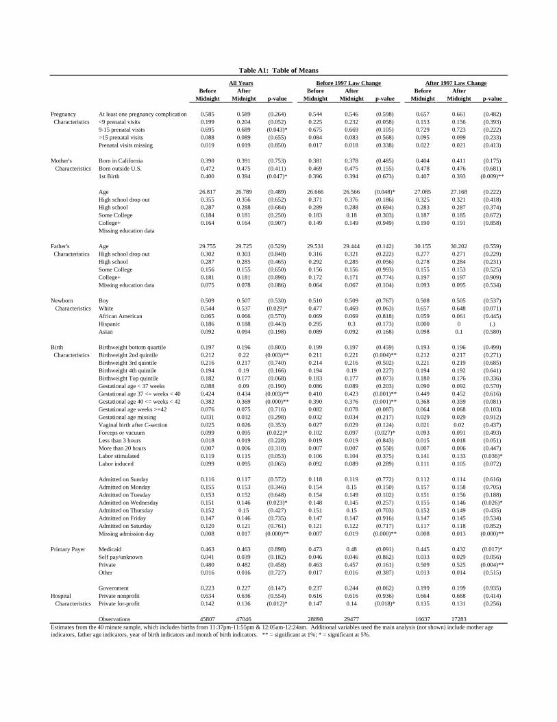
Before After Before After Before AfterMidnight Midnight p-value Midnight Midnight p-value Midnight Midnight p-value

Pregnancy At least one pregnancy complication 0.585 0.589 (0.264) 0.544 0.546 (0.598) 0.657 0.661 (0.482) Characteristics <9 prenatal visits 0.199 0.204 (0.052) 0.225 0.232 (0.058) 0.153 0.156 (0.393)

9-15 prenatal visits 0.695 0.689 (0.043)* 0.675 0.669 (0.105) 0.729 0.723 (0.222)>15 prenatal visits 0.088 0.089 (0.655) 0.084 0.083 (0.568) 0.095 0.099 (0.233)Prenatal visits missing 0.019 0.019 (0.850) 0.017 0.018 (0.338) 0.022 0.021 (0.413)

Mother's Born in California 0.390 0.391 (0.753) 0.381 0.378 (0.485) 0.404 0.411 (0.175) Characteristics Born outside U.S. 0.472 0.475 (0.411) 0.469 0.475 (0.155) 0.478 0.476 (0.681)

1st Birth 0.400 0.394 (0.047)* 0.396 0.394 (0.673) 0.407 0.393 (0.009)**

Age 26.817 26.789 (0.489) 26.666 26.566 (0.048)* 27.085 27.168 (0.222)High school drop out 0.355 0.356 (0.652) 0.371 0.376 (0.186) 0.325 0.321 (0.418)High school 0.287 0.288 (0.684) 0.289 0.288 (0.694) 0.283 0.287 (0.374)Some College 0.184 0.181 (0.250) 0.183 0.18 (0.303) 0.187 0.185 (0.672)College+ 0.164 0.164 (0.907) 0.149 0.149 (0.949) 0.190 0.191 (0.858)Missing education data

Father's Age 29.755 29.725 (0.529) 29.531 29.444 (0.142) 30.155 30.202 (0.559) Characteristics High school drop out 0.302 0.303 (0.848) 0.316 0.321 (0.222) 0.277 0.271 (0.229)

High school 0.287 0.285 (0.465) 0.292 0.285 (0.056) 0.278 0.284 (0.231)Some College 0.156 0.155 (0.650) 0.156 0.156 (0.993) 0.155 0.153 (0.525)College+ 0.181 0.181 (0.898) 0.172 0.171 (0.774) 0.197 0.197 (0.909)Missing education data 0.075 0.078 (0.086) 0.064 0.067 (0.104) 0.093 0.095 (0.534)

Newborn Boy 0.509 0.507 (0.530) 0.510 0.509 (0.767) 0.508 0.505 (0.537) Characteristics White 0.544 0.537 (0.029)* 0.477 0.469 (0.063) 0.657 0.648 (0.071)

African American 0.065 0.066 (0.570) 0.069 0.069 (0.818) 0.059 0.061 (0.445)Hispanic 0.186 0.188 (0.443) 0.295 0.3 (0.173) 0.000 0 (.)Asian 0.092 0.094 (0.198) 0.089 0.092 (0.168) 0.098 0.1 (0.580)

Birth Birthweight bottom quartile 0.197 0.196 (0.803) 0.199 0.197 (0.459) 0.193 0.196 (0.499) Characteristics Birthweight 2nd quintile 0.212 0.22 (0.003)** 0.211 0.221 (0.004)** 0.212 0.217 (0.271)

Birthweight 3rd quintile 0.216 0.217 (0.740) 0.214 0.216 (0.502) 0.221 0.219 (0.685)Birthweight 4th quintile 0.194 0.19 (0.166) 0.194 0.19 (0.227) 0.194 0.192 (0.641)Birthweight Top quintile 0.182 0.177 (0.068) 0.183 0.177 (0.073) 0.180 0.176 (0.336)Gestational age < 37 weeks 0.088 0.09 (0.190) 0.086 0.089 (0.203) 0.090 0.092 (0.570)Gestational age 37 <= weeks < 40 0.424 0.434 (0.003)** 0.410 0.423 (0.001)** 0.449 0.452 (0.616)Gestational age 40 <= weeks < 42 0.382 0.369 (0.000)** 0.390 0.376 (0.001)** 0.368 0.359 (0.081)Gestational age weeks >=42 0.076 0.075 (0.716) 0.082 0.078 (0.087) 0.064 0.068 (0.103)Gestational age missing 0.031 0.032 (0.298) 0.032 0.034 (0.217) 0.029 0.029 (0.912)Vaginal birth after C-section 0.025 0.026 (0.353) 0.027 0.029 (0.124) 0.021 0.02 (0.437)Forceps or vacuum 0.099 0.095 (0.022)* 0.102 0.097 (0.027)* 0.093 0.091 (0.493)Less than 3 hours 0.018 0.019 (0.228) 0.019 0.019 (0.843) 0.015 0.018 (0.051)More than 20 hours 0.007 0.006 (0.310) 0.007 0.007 (0.550) 0.007 0.006 (0.447)Labor stimulated 0.119 0.115 (0.053) 0.106 0.104 (0.375) 0.141 0.133 (0.036)*Labor induced 0.099 0.095 (0.065) 0.092 0.089 (0.289) 0.111 0.105 (0.072)

Admitted on Sunday 0.116 0.117 (0.572) 0.118 0.119 (0.772) 0.112 0.114 (0.616)Admitted on Monday 0.155 0.153 (0.346) 0.154 0.15 (0.150) 0.157 0.158 (0.705)Admitted on Tuesday 0.153 0.152 (0.648) 0.154 0.149 (0.102) 0.151 0.156 (0.188)Admitted on Wednesday 0.151 0.146 (0.023)* 0.148 0.145 (0.257) 0.155 0.146 (0.026)*Admitted on Thursday 0.152 0.15 (0.427) 0.151 0.15 (0.703) 0.152 0.149 (0.435)Admitted on Friday 0.147 0.146 (0.735) 0.147 0.147 (0.916) 0.147 0.145 (0.534)Admitted on Saturday 0.120 0.121 (0.761) 0.121 0.122 (0.717) 0.117 0.118 (0.852)Missing admission day 0.008 0.017 (0.000)** 0.007 0.019 (0.000)** 0.008 0.013 (0.000)**

Primary Payer Medicaid 0.463 0.463 (0.898) 0.473 0.48 (0.091) 0.445 0.432 (0.017)*Self pay/unknown 0.041 0.039 (0.182) 0.046 0.046 (0.862) 0.033 0.029 (0.056)Private 0.480 0.482 (0.458) 0.463 0.457 (0.161) 0.509 0.525 (0.004)**Other 0.016 0.016 (0.727) 0.017 0.016 (0.387) 0.013 0.014 (0.515)

Government 0.223 0.227 (0.147) 0.237 0.244 (0.062) 0.199 0.199 (0.935)Hospital Private nonprofit 0.634 0.636 (0.554) 0.616 0.616 (0.936) 0.664 0.668 (0.414) Characteristics Private for-profit 0.142 0.136 (0.012)* 0.147 0.14 (0.018)* 0.135 0.131 (0.256)

Observations 45807 47046 28898 29477 16637 17283

All Years

Estimates from the 40 minute sample, which includes births from 11:37pm-11:55pm & 12:05am-12:24am. Additional variables used the main analysis (not shown) include mother age indicators, father age indicators, year of birth indicators and month of birth indicators. ** = significant at 1%; * = significant at 5%.

Table A1: Table of Means

Before 1997 Law Change After 1997 Law Change

Dependent Variable: Additional Midnights 28-Day Readmission 1-year Mortality(1) (2) (3)

Birth After Midnight 0.255 0.0023 0.00036(0.025)** (0.0026) (0.00035)

Birth After Midnight * Minute from cutoff 0.001 0.0001 -0.00001(0.002) (0.0002) (0.00002)

Birth Prior to Midnight* Minute from cutoff -0.002 -0.0001 -0.00003(0.002) (0.0002) (0.00002)

Pregnancy At least one pregnancy complication 0.021 -0.0006 0.00050 Characterisitics (0.014) (0.0014) (0.00018)**

9-15 prenatal visits -0.073 -0.0022 -0.00217 (<9 omitted) (0.020)** (0.0017) (0.00029)**

>15 prenatal visits 0.055 0.0019 -0.00107(0.029) (0.0027) (0.00018)**

Prenatal visits missing 0.060 0.0042 -0.00014(0.060) (0.0051) (0.00044)

Mother's Born in California 0.023 0.0005 0.00011 Characteristics (0.021) (0.0021) (0.00026)

Born outside U.S. 0.028 -0.0047 -0.00075(0.023) (0.0024)* (0.00029)*

1st Birth 0.232 0.0063 0.00004(0.016)** (0.0016)** (0.00020)

(Age<18 omitted) Age = 20 -0.057 0.0028 0.00121(0.046) (0.0047) (0.00090)

Age = 30 0.219 0.0026 0.00094(0.053)** (0.0051) (0.00092)

Age = 40 0.315 0.0119 0.00028(0.071)** (0.0075) (0.00091)

(College+ omitted) High school drop out 0.034 0.0011 0.00028(0.027) (0.0031) (0.00042)

High school 0.004 -0.0005 -0.00012(0.023) (0.0027) (0.00034)

Some College 0.009 0.0013 0.00018(0.021) (0.0026) (0.00037)

Missing education data 0.147 0.0016 0.00220(0.091) (0.0074) (0.00174)

Father's Age = 20 0.080 0.0071 -0.00043 Characterisitcs (0.076) (0.0084) (0.00057)

Age = 30 0.083 0.0041 -0.00042 (Age<18 omitted) (0.074) (0.0080) (0.00058)

Age = 40 0.183 0.0055 -0.00071(0.075)* (0.0080) (0.00046)

Age Missing 0.203 0.0044 -0.00021(0.075)** (0.0076) (0.00065)

High school drop out 0.007 -0.0026 0.00013 (College+ omitted) (0.026) (0.0029) (0.00039)

High school 0.014 -0.0030 -0.00017(0.023) (0.0025) (0.00033)

Some College -0.038 0.0019 0.00025(0.021) (0.0026) (0.00037)

Missing education data 0.052 0.0014 -0.00037(0.044) (0.0040) (0.00038)

Mean of Dependent Variable 1.10 0.044 0.0050Observations 92853 92853 92802

Table A2: Selected Covariates: 40 Minute Pooled Sample, 1991-2002

Additional characteristics included month, year, day of the week, mother's age, and father's age indicators. ** = significant at 1%; * = significant at 5%.

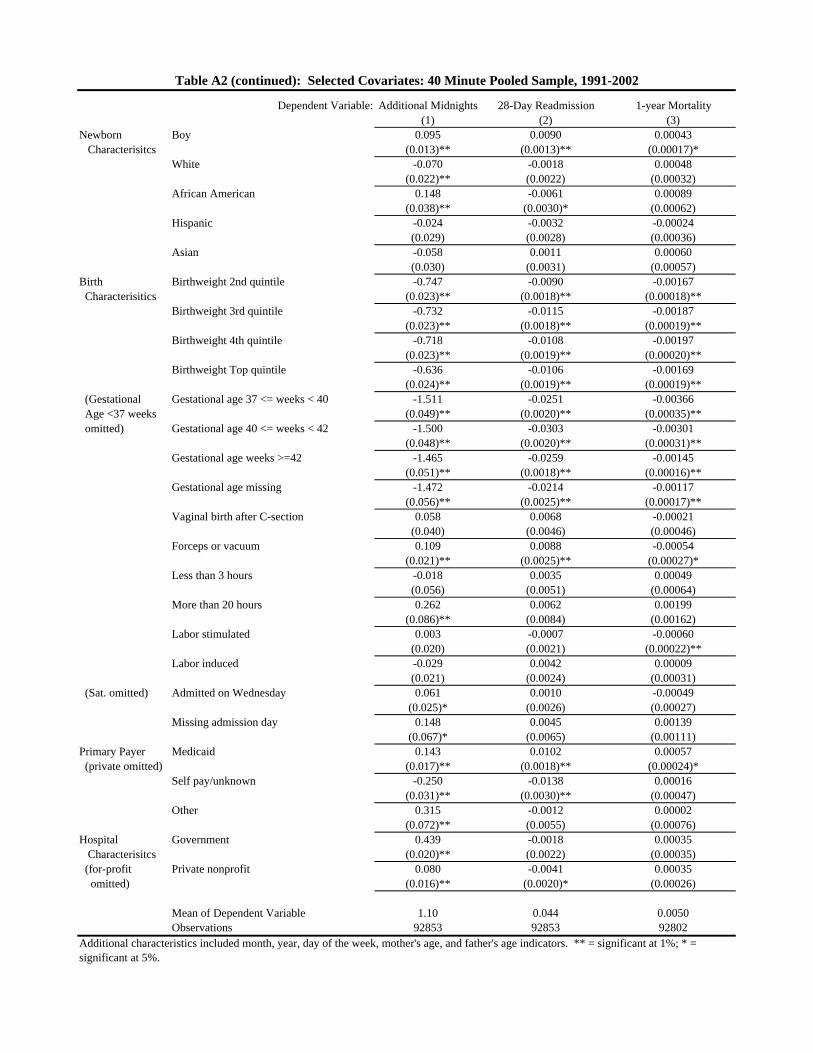
Dependent Variable: Additional Midnights 28-Day Readmission 1-year Mortality(1) (2) (3)

Newborn Boy 0.095 0.0090 0.00043 Characterisitcs (0.013)** (0.0013)** (0.00017)*

White -0.070 -0.0018 0.00048(0.022)** (0.0022) (0.00032)

African American 0.148 -0.0061 0.00089(0.038)** (0.0030)* (0.00062)

Hispanic -0.024 -0.0032 -0.00024(0.029) (0.0028) (0.00036)

Asian -0.058 0.0011 0.00060(0.030) (0.0031) (0.00057)

Birth Birthweight 2nd quintile -0.747 -0.0090 -0.00167 Characterisitics (0.023)** (0.0018)** (0.00018)**

Birthweight 3rd quintile -0.732 -0.0115 -0.00187(0.023)** (0.0018)** (0.00019)**

Birthweight 4th quintile -0.718 -0.0108 -0.00197(0.023)** (0.0019)** (0.00020)**

Birthweight Top quintile -0.636 -0.0106 -0.00169(0.024)** (0.0019)** (0.00019)**

(Gestational Gestational age 37 <= weeks < 40 -1.511 -0.0251 -0.00366 Age <37 weeks (0.049)** (0.0020)** (0.00035)** omitted) Gestational age 40 <= weeks < 42 -1.500 -0.0303 -0.00301

(0.048)** (0.0020)** (0.00031)**Gestational age weeks >=42 -1.465 -0.0259 -0.00145

(0.051)** (0.0018)** (0.00016)**Gestational age missing -1.472 -0.0214 -0.00117

(0.056)** (0.0025)** (0.00017)**Vaginal birth after C-section 0.058 0.0068 -0.00021

(0.040) (0.0046) (0.00046)Forceps or vacuum 0.109 0.0088 -0.00054

(0.021)** (0.0025)** (0.00027)*Less than 3 hours -0.018 0.0035 0.00049

(0.056) (0.0051) (0.00064)More than 20 hours 0.262 0.0062 0.00199

(0.086)** (0.0084) (0.00162)Labor stimulated 0.003 -0.0007 -0.00060

(0.020) (0.0021) (0.00022)**Labor induced -0.029 0.0042 0.00009

(0.021) (0.0024) (0.00031) (Sat. omitted) Admitted on Wednesday 0.061 0.0010 -0.00049

(0.025)* (0.0026) (0.00027)Missing admission day 0.148 0.0045 0.00139

(0.067)* (0.0065) (0.00111)Primary Payer Medicaid 0.143 0.0102 0.00057 (private omitted) (0.017)** (0.0018)** (0.00024)*

Self pay/unknown -0.250 -0.0138 0.00016(0.031)** (0.0030)** (0.00047)

Other 0.315 -0.0012 0.00002(0.072)** (0.0055) (0.00076)

Hospital Government 0.439 -0.0018 0.00035 Characterisitcs (0.020)** (0.0022) (0.00035) (for-profit Private nonprofit 0.080 -0.0041 0.00035 omitted) (0.016)** (0.0020)* (0.00026)

Mean of Dependent Variable 1.10 0.044 0.0050Observations 92853 92853 92802

Table A2 (continued): Selected Covariates: 40 Minute Pooled Sample, 1991-2002

Additional characteristics included month, year, day of the week, mother's age, and father's age indicators. ** = significant at 1%; * = significant at 5%.

A. Before the Law Change

Coeff. On Mean of Marginal effect of Mean of Marginal effect of Mean ofAfter Midnight S.E. Dep. Var. After Midnight S.E. Dep. Var. After Midnight S.E. Dep. Var. Obs.

Subgroup:Medicaid Patient 0.25831 (0.02984)** 1.10 0.00414 (0.00294) 0.047 -0.00013 (0.00054) 0.0062 77272

Unmarried 0.25165 (0.0360)** 1.09 0.00146 (.000332) 0.044 0.00017 (0.00063) 0.0060 56440

For-Profit Hospital 0.23857 (0.03859)** 0.79 -0.00138 (0.00493) 0.044 0.00009 (0.00039) 0.0041 19765

Cesarean Section 0.23909 (0.06236)** 2.87 0.00376 (0.00428) 0.049 -0.00208 (0.00089)* 0.0094 34442

Birthweight < 3000g 0.22649 (0.07206)** 1.71 0.00654 (0.00479) 0.060 -0.00024 (0.00148) 0.0183 34675

High P(Readmission|X) 0.21937 (0.03615)** 1.25 0.00285 (0.00318) 0.055 0.00019 (0.00060) 0.00944 77012

Low P(Readmission|X) 0.21634 (0.01584)** 0.72 0.00264 (0.00237) 0.031 -0.00022 (0.00039) 0.00191 85319

Low Maternal Education 0.18903 (0.03297)** 1.07 0.00375 (0.00317) 0.043 -0.00065 (0.00063) 0.0060 60403

Kaiser Hospital 0.18820 (0.05150)** 0.91 0.00768 (0.00510) 0.035 0.0005 (0.00062) 0.0062 19616

Any Labor Complication 0.18372 (0.02364)** 0.97 0.00549 (0.00236)* 0.042 0.00018 (0.00039) 0.0060 108265

Scheduled Birth 0.16825 (0.05151)** 0.75 -0.00064 (0.00608) 0.049 0.00008 (0.00021) 0.0037 15225

Any Pregnancy Complication 0.16427 (0.02678)** 0.98 0.00455 (0.00263) 0.044 0.00030 (0.00045) 0.0063 88955

All Data 0.13561 (0.05248)** 1.81 0.00210 (0.00163) 0.043 -0.00025 (0.00033) 0.0065 229554

B. After the Law Change

Coeff. On Mean of Coeff. On Mean of Coeff. On Mean ofAfter Midnight S.E. Dep. Var. After Midnight S.E. Dep. Var. After Midnight S.E. Dep. Var. Obs.

Subgroup:Medicaid Patient 0.26693 (0.03925)** 1.35 0.00464 (0.00415) 0.049 0.00027 (0.00046) 0.0051 41412

Unmarried 0.24456 (0.07785)** 1.28 0.00486 (0.00735) 0.050 -0.00019 (0.00032) 0.0076 6374

For-Profit Hospital 0.31748 (0.05329)** 1.07 -0.00175 (0.00661) 0.052 -0.00021 (0.00027) 0.0086 5547

Cesarean Section 0.22570 (0.08319)** 3.14 0.00909 (0.00570) 0.052 -0.00027 (0.00083) 0.0074 20777

Birthweight < 3000g 0.09485 (0.09228) 2.05 0.00836 (0.00636) 0.063 -0.00026 (0.00129) 0.0168 19937

High P(Readmission|X) 0.26061 (0.04092)** 1.49 -0.00017 (0.00397) 0.057 -0.00026 (0.00037) 0.00756 51520

Low P(Readmission|X) 0.22471 (0.02251)** 1.01 -0.00214 (0.00332) 0.033 0.00077 (0.00052) 0.00226 27239

Low Maternal Education 0.24245 (0.04515)** 1.29 0.00656 (0.00459) 0.045 0.00061 (0.00042) 0.0044 29431

Kaiser Hospital 0.08651 (0.05824) 1.15 -0.00559 (0.00538) 0.034 -0.000002 (0.00014) 0.0057 11176

Any Labor Complication 0.24057 (0.02893)** 1.27 -0.00004 (0.00305) 0.046 0.00010 (0.00031) 0.0050 69767

Scheduled Birth 0.27764 (0.04104)** 1.21 0.00201 (0.00419) 0.041 0.00050 (0.00044) 0.0038 30303

Any Pregnancy Complication 0.23126 (0.03095)** 1.28 -0.00033 (0.00325) 0.048 0.00001 (0.00037) 0.0055 62285

All Data 0.29971 (0.06152)** 2.10 0.00020 (0.00196) 0.045 0.00029 (0.00031) 0.0055 162427Analyses use the 2 hour sample, which includes births from 11:02pm-11:55pm & 12:05am to 12:59am. The additional midnight models are estimated by OLS, and the readmission and mortality columns report marginal effects from a probit model, evaluated at the mean of the covariates. Models for unmarried do not include missing observations and only include 2 years in the post-law change period. Robust standard errors reported in parentheses. All models include full controls listed in Appendix Table A1, as well as mother age indicators, father age indicators, year of birth indicators and month of birth indicators. Number of observations listed is for the mortality model, which is a lower bound on the number of observations in that row, as some cells have zero deaths. ** = significant at 1%; * = significant at 5%.

Appendix Table A3: Infant Outcomes Across Patient Groups

Additional Midnights 28-Day Readmission 1-year Mortality

Additional Midnights 28-Day Readmission 1-year Mortality

24-hour 24-hourComplier Overall Population Complier Overall Population

Mean Mean Mean Mean Mean Mean

Pregnancy At least one pregnancy complication 0.546 0.545 0.565 0.683 0.659 0.664 Characteristics <9 prenatal visits 0.202 0.228 0.208 0.129 0.155 0.137

9-15 prenatal visits 0.699 0.672 0.685 0.696 0.726 0.734>15 prenatal visits 0.078 0.083 0.091 0.147 0.097 0.109Prenatal visits missing 0.021 0.017 0.016 0.028 0.021 0.021

Mother's Born in California 0.380 0.380 0.391 0.396 0.407 0.414 Characteristics Born outside U.S. 0.482 0.472 0.455 0.490 0.476 0.460

1st Birth 0.385 0.395 0.391 0.414 0.400 0.387

Age 26.2 26.6 27.1 28.3 27.1 27.8High school drop out 0.387 0.374 0.346 0.297 0.323 0.298High school 0.274 0.289 0.291 0.237 0.285 0.282Some College 0.177 0.181 0.191 0.198 0.186 0.193College+ 0.156 0.149 0.165 0.252 0.191 0.213Missing education data 0.006 0.007 0.007 0.015 0.015 0.014

Father's Age 28.9 29.5 29.9 31.4 30.2 30.7 Characteristics High school drop out 0.312 0.319 0.299 0.232 0.274 0.256

High school 0.259 0.289 0.290 0.253 0.281 0.276Some College 0.176 0.156 0.163 0.160 0.154 0.162College+ 0.169 0.171 0.187 0.254 0.198 0.220Missing education data 0.083 0.065 0.061 0.100 0.094 0.086

Newborn Boy 0.496 0.509 0.510 0.482 0.506 0.510 Characteristics White 0.466 0.473 0.508 0.615 0.652 0.681

African American 0.073 0.069 0.069 0.075 0.060 0.060Hispanic 0.299 0.298 0.260 . .Asian 0.091 0.091 0.091 0.124 0.098 0.095

Birth Low birthweight (<2500g) 0.005 0.048 0.059 0.029 0.047 0.061 Characteristics Full Term (>=37 weeks) 0.927 0.909 0.898 0.915 0.906 0.896

Vaginal birth after C-section 0.035 0.028 0.022 0.023 0.021 0.015Forceps or vacuum 0.077 0.099 0.083 0.102 0.092 0.072Less than 3 hours 0.019 0.020 0.014 0.016 0.016 0.011More than 20 hours 0.002 0.007 0.008 0.009 0.006 0.007Labor stimulated 0.085 0.105 0.097 0.124 0.137 0.116Labor induced 0.089 0.091 0.087 0.101 0.108 0.109Admitted on a weekend 0.266 0.243 0.228 0.261 0.233 0.216

Primary Payer Medicaid 0.489 0.477 0.457 0.425 0.439 0.417Self pay/unknown 0.038 0.046 0.045 0.009 0.031 0.027Private 0.459 0.460 0.481 0.550 0.517 0.540Other 0.014 0.016 0.018 0.016 0.014 0.016

Government 0.222 0.241 0.215 0.264 0.200 0.183Hospital Private nonprofit 0.644 0.616 0.630 0.585 0.666 0.666 Characteristics Private for-profit 0.134 0.143 0.153 0.152 0.133 0.149

Excluded Cesarean Section . . 0.215 . . 0.240 Characteristics

Observations 3455661 2561629Compliers are newborns who are induced into having a longer stay due to a post-midnight births, where longer stays are defined as at least one additional midnight prior to the law change and at least 2 additional midnights after the law change. The means are then calculated as described in the text. The 40-minute sample is the analysis sample used in Table 3. The 24-hour population includes all births in California hospitals. The estimated fraction of compliers in the 40-minute sample is 16% prior to the law change and 17% after the law change.

40-minute Sample40-minute SampleBefore Law Change

Appendix Table A4: Characteristics of Compliers

58375 33920

After Law Change

Figure 1: Average Length of U.S. Hospital Stay by Type of Delivery

0

1

2

3

4

5

6

7

8

9

1970 1972 1974 1976 1978 1980 1982 1984 1986 1988 1990 1992 1994 1996 1998 2000 2002 2004

Year

Day

s in

hosp

ital

vaginalcesarean

Figure 2: Vaginal Births: Less Than 2 Days in the Hospital

0

0.1

0.2

0.3

0.4

0.5

1970 1972 1974 1976 1978 1980 1982 1984 1986 1988 1990 1992 1994 1996 1998 2000 2002 2004

Year

Perc

ent o

f Vag

inal

Birt

hs

1995

Figure 3: California Vaginal Births: Less than 2 Days in the Hospital

0%

10%

20%

30%

40%

50%

60%

70%

80%

90%

01/01/91 12/14/91 11/25/92 11/07/93 10/20/94 10/02/95 09/13/96 08/26/97 08/08/98 07/21/99 07/02/00 06/14/01 05/27/02

Birth Date

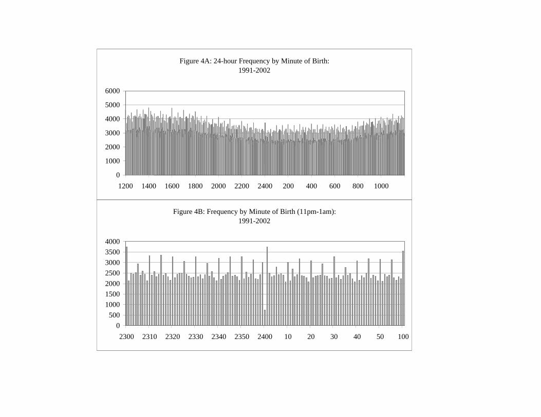
Figure 4A: 24-hour Frequency by Minute of Birth: 1991-2002

0

1000

2000

3000

4000

5000

6000

1200 1400 1600 1800 2000 2200 2400 200 400 600 800 1000

Figure 4B: Frequency by Minute of Birth (11pm-1am): 1991-2002

0500

1000150020002500300035004000

2300 2310 2320 2330 2340 2350 2400 10 20 30 40 50 100

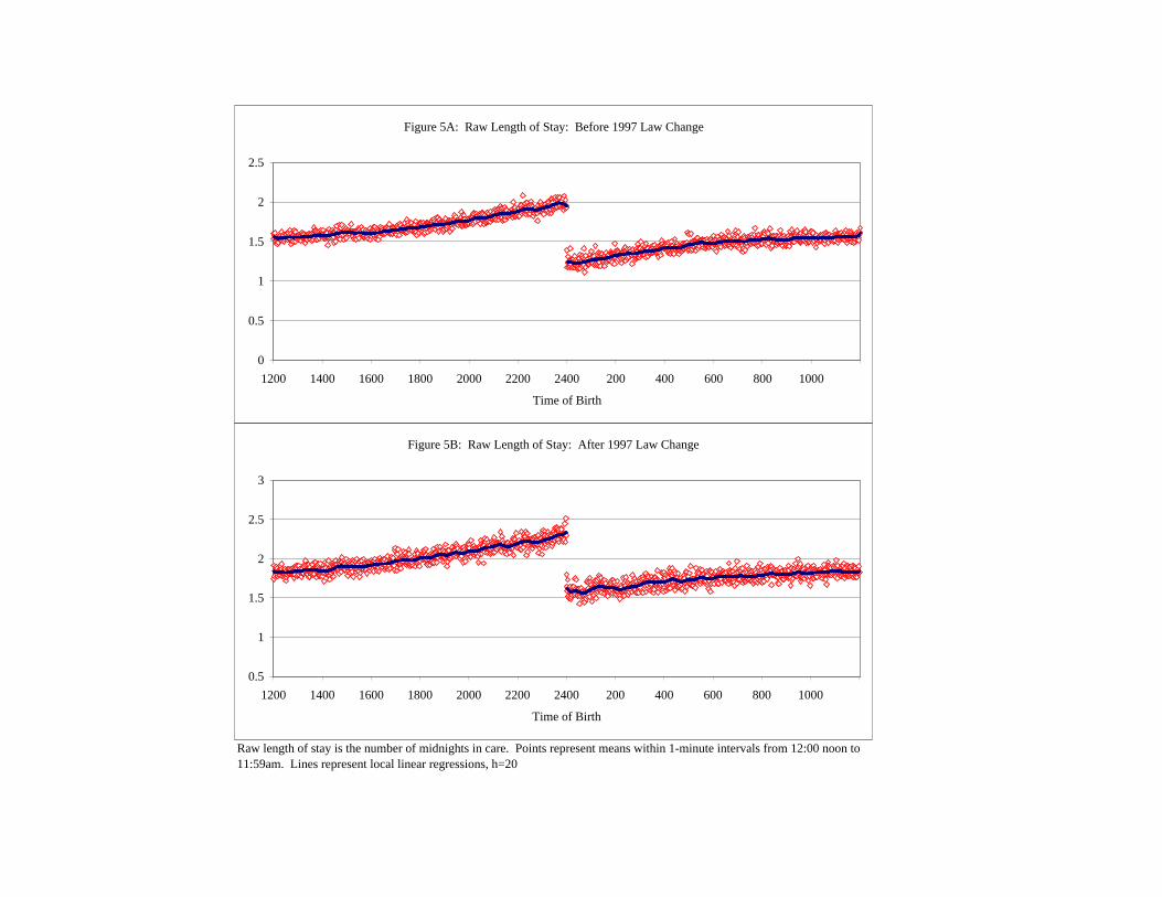
Raw length of stay is the number of midnights in care. Points represent means within 1-minute intervals from 12:00 noon to 11:59am. Lines represent local linear regressions, h=20

Figure 5A: Raw Length of Stay: Before 1997 Law Change

0

0.5

1

1.5

2

2.5

1200 1400 1600 1800 2000 2200 2400 200 400 600 800 1000

Time of Birth

Figure 5B: Raw Length of Stay: After 1997 Law Change

0.5

1

1.5

2

2.5

3

1200 1400 1600 1800 2000 2200 2400 200 400 600 800 1000

Time of Birth

Number of additional midnights is the number of midnights for those born on or after midnight and before noon, while the number of additional midnights is measured as the number of midnights minus one for children born after noon and before midnight. Points represent means within 1-minute intervals from 12:00 noon to 11:59am. Lines represent local linear regressions, h=20

Figure 6A: Additional Midnights: Before Law Change

0.5

0.8

1.1

1.4

1.7

2

1200 1400 1600 1800 2000 2200 2400 200 400 600 800 1000

Minute of Birth

Figure 6B: 1 or More Additional Midnights: Before Law Change

00.10.20.30.40.50.60.70.80.9

1

1200 1400 1600 1800 2000 2200 2400 200 400 600 800 1000

Minute of Birth

Figure 6C: 2 or More Additional Midnights: Before Law Change

0

0.1

0.2

0.3

0.4

0.5

0.6

1200 1400 1600 1800 2000 2200 2400 200 400 600 800 1000

Minute of Birth

Number of additional midnights is the number of midnights for those born on or after midnight and before noon, while the number of additional midnights is measured as the number of midnights minus one for children born after noon and before midnight. Points represent means within 1-minute intervals from 12:00 noon to 11:59am. Lines represent local linear regressions, h=20

Figure 7A: Additional Midnights: After Law Change

0.5

0.8

1.1

1.4

1.7

2

1200 1400 1600 1800 2000 2200 2400 200 400 600 800 1000

Minute of Birth

Figure 7B: 1 or More Additional Midnights: After Law Change

00.10.20.30.40.50.60.70.80.9

1

1200 1400 1600 1800 2000 2200 2400 200 400 600 800 1000

Minute of Birth

Figure 7C: 2 or More Additional Midnights: After Law Change

0

0.1

0.2

0.3

0.4

0.5

0.6

1200 1400 1600 1800 2000 2200 2400 200 400 600 800 1000

Minute of Birth

28-day measures consider 28 days since the midnight prior to those born between midnight and noon, and 28 days since the following midnight for those born between noon and midnight. An analogous consideration was made for 7-day readmissions. Points represent means within 1-minute intervals from 12:00 noon to 11:59am. Lines represent local linear regressions, h=20

Figure 8A: 7-Day Readmission Rate: Before Law Change

00.005

0.010.015

0.020.025

0.030.035

0.040.045

0.05

1200 1400 1600 1800 2000 2200 2400 200 400 600 800 1000

Time of Birth

Figure 8C: Infant Mortality Rate: Before Law Change

0

0.002

0.004

0.006

0.008

0.01

0.012

0.014

1200 1400 1600 1800 2000 2200 2400 200 400 600 800 1000

Time of Birth

Figure 8B: 28-Day Readmission Rate: Before Law Change

0

0.01

0.02

0.03

0.04

0.05

0.06

0.07

0.08

1200 1400 1600 1800 2000 2200 2400 200 400 600 800 1000

Time of Birth

Figure 8D: 28-Day Mortality Rate: Before Law Change

0

0.002

0.004

0.006

0.008

0.01

0.012

1200 1400 1600 1800 2000 2200 2400 200 400 600 800 1000

Time of Birth

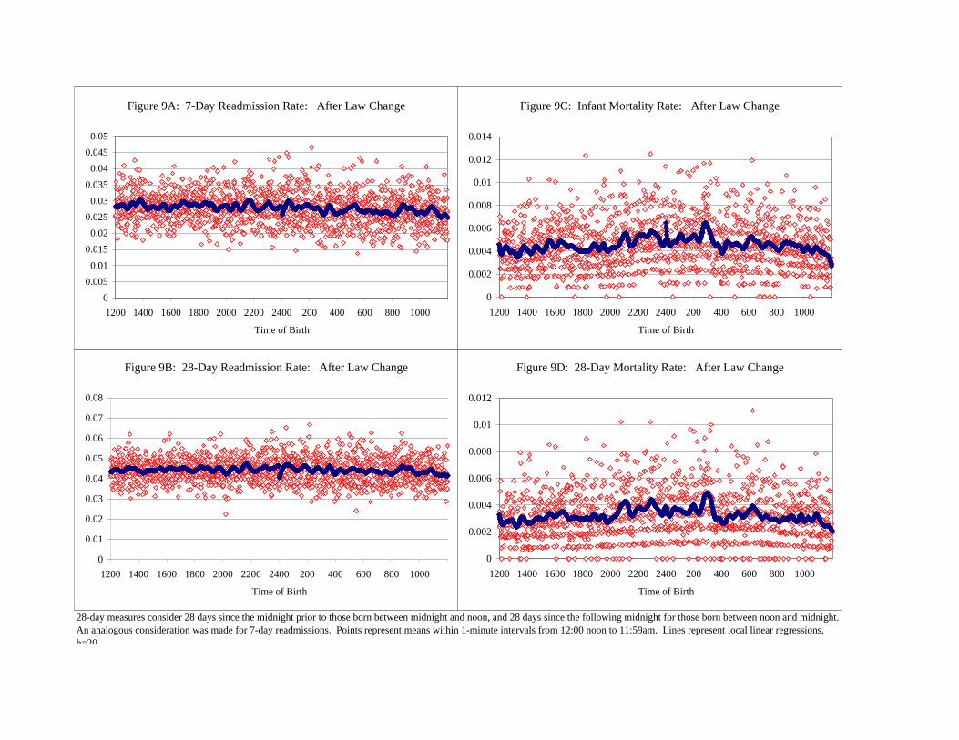
28-day measures consider 28 days since the midnight prior to those born between midnight and noon, and 28 days since the following midnight for those born between noon and midnight. An analogous consideration was made for 7-day readmissions. Points represent means within 1-minute intervals from 12:00 noon to 11:59am. Lines represent local linear regressions, h=20

Figure 9A: 7-Day Readmission Rate: After Law Change

00.005

0.010.015

0.020.025

0.030.035

0.040.045

0.05

1200 1400 1600 1800 2000 2200 2400 200 400 600 800 1000

Time of Birth

Figure 9C: Infant Mortality Rate: After Law Change

0

0.002

0.004

0.006

0.008

0.01

0.012

0.014

1200 1400 1600 1800 2000 2200 2400 200 400 600 800 1000

Time of Birth

Figure 9B: 28-Day Readmission Rate: After Law Change

0

0.01

0.02

0.03

0.04

0.05

0.06

0.07

0.08

1200 1400 1600 1800 2000 2200 2400 200 400 600 800 1000

Time of Birth

Figure 9D: 28-Day Mortality Rate: After Law Change

0

0.002

0.004

0.006

0.008

0.01

0.012

1200 1400 1600 1800 2000 2200 2400 200 400 600 800 1000

Time of Birth

Figure A1A: Bandwidth of 10: Additional Midnights Before Law Change

0.5

0.8

1.1

1.4

1.7

2

2000 2100 2200 2300 2400 100 200 300 400

Minute of Birth

Figure A1B: Bandwidth of 10: Additional Midnights After Law Change

0.5

0.8

1.1

1.4

1.7

2

2000 2100 2200 2300 2400 100 200 300 400

Minute of Birth

Figure A2A: Bandwidth of 10:7-Day Readmission Rate Before Law Change

00.005

0.010.015

0.020.025

0.030.035

0.040.045

0.05

2000 2100 2200 2300 2400 100 200 300 400

Time of Birth

Figure A2B: Bandwidth of 10:28-Day Readmission Rate: Before Law Change

0

0.01

0.02

0.03

0.04

0.05

0.06

0.07

0.08

2000 2100 2200 2300 2400 100 200 300 400

Time of Birth

Figure A2C: Bandwidth of 10:Infant Mortality Rate: Before Law Change

0

0.002

0.004

0.006

0.008

0.01

0.012

0.014

2000 2100 2200 2300 2400 100 200 300 400

Time of Birth

Figure A2D: Bandwidth of 10: 28-Day Mortality Rate: Before Law Change

0

0.002

0.004

0.006

0.008

0.01

0.012

2000 2100 2200 2300 2400 100 200 300 400

Time of Birth

28-day measures consider 28 days since the midnight being compared. Points represent means within 1-minute intervals, lines represent local linear regressions, h=10

Figure A3C: Bandwidth of 10: Infant Mortality Rate: After Law Change

0

0.002

0.004

0.006

0.008

0.01

0.012

0.014

2000 2100 2200 2300 2400 100 200 300

Time of Birth

Figure A3D: Bandwidth of 10: 28-Day Mortality Rate: After Law Change

0

0.002

0.004

0.006

0.008

0.01

0.012

2000 2100 2200 2300 2400 100 200 300

Time of Birth

Figure A3A: Bandwidth of 10: 7-Day Readmission Rate: After Law Change

00.005

0.010.015

0.020.025

0.030.035

0.040.045

0.05

2000 2100 2200 2300 2400 100 200 300

Time of Birth

Figure A3B: Bandwidth of 10: 28-Day Readmission Rate: After Law Change

0

0.01

0.02

0.03

0.04

0.05

0.06

0.07

0.08

2000 2100 2200 2300 2400 100 200 300

Time of Birth