AFRL-RX-WP-TP-2010-4058

PROBABILISTIC FRETTING FATIGUE LIFE PREDICTION OF Ti-6Al-4V (PREPRINT) Patrick J. Golden Metals Branch Metals, Ceramics & NDE Division Harry R. Millwater and Xiaobin Yang University of Texas at San Antonio

JANUARY 2010

Approved for public release; distribution unlimited. See additional restrictions described on inside pages

STINFO COPY

AIR FORCE RESEARCH LABORATORY MATERIALS AND MANUFACTURING DIRECTORATE

WRIGHT-PATTERSON AIR FORCE BASE, OH 45433-7750 AIR FORCE MATERIEL COMMAND

UNITED STATES AIR FORCE

i

REPORT DOCUMENTATION PAGE Form Approved

OMB No. 0704-0188

The public reporting burden for this collection of information is estimated to average 1 hour per response, including the time for reviewing instructions, searching existing data sources, gathering and maintaining the data needed, and completing and reviewing the collection of information. Send comments regarding this burden estimate or any other aspect of this collection of information, including suggestions for reducing this burden, to Department of Defense, Washington Headquarters Services, Directorate for Information Operations and Reports (0704-0188), 1215 Jefferson Davis Highway, Suite 1204, Arlington, VA 22202-4302. Respondents should be aware that notwithstanding any other provision of law, no person shall be subject to any penalty for failing to comply with a collection of information if it does not display a currently valid OMB control number. PLEASE DO NOT RETURN YOUR FORM TO THE ABOVE ADDRESS.

1. REPORT DATE (DD-MM-YY) 2. REPORT TYPE 3. DATES COVERED (From - To)

January 2010 Journal Article Preprint 01 January 2010 – 31 January 2010 4. TITLE AND SUBTITLE

PROBABILISTIC FRETTING FATIGUE LIFE PREDICTION OF Ti-6Al-4V (PREPRINT)

5a. CONTRACT NUMBER

FA8650-04-C-5200 5b. GRANT NUMBER

5c. PROGRAM ELEMENT NUMBER

62102F 6. AUTHOR(S)

Patrick J. Golden (AFRL/RXLM) Harry R. Millwater and Xiaobin Yang (University of Texas at San Antonio)

5d. PROJECT NUMBER

4347 5e. TASK NUMBER

RG 5f. WORK UNIT NUMBER

M02R3000 7. PERFORMING ORGANIZATION NAME(S) AND ADDRESS(ES) 8. PERFORMING ORGANIZATION

Metals Branch (AFRL/RXLM) Metals, Ceramics & NDE Division Materials and Manufacturing Directorate Wright-Patterson Air Force Base, OH 45433-7750 Air Force Materiel Command, United States Air Force

University of Texas at San Antonio San Antonio, TX 78249

REPORT NUMBER

9. SPONSORING/MONITORING AGENCY NAME(S) AND ADDRESS(ES)

Air Force Research Laboratory

10. SPONSORING/MONITORING AGENCY ACRONYM(S)

Materials and Manufacturing Directorate Wright-Patterson Air Force Base, OH 45433-7750 Air Force Materiel Command United States Air Force

AFRL/RXLMN 11. SPONSORING/MONITORING AGENCY REPORT NUMBER(S)

AFRL-RX-WP-TP-2010-4058

12. DISTRIBUTION/AVAILABILITY STATEMENT

Approved for public release; distribution unlimited.

13. SUPPLEMENTARY NOTES

Journal article submitted to International Journal of Fatigue. PAO Case Number: 88ABW-2009-4305; Clearance Date: 07 Oct 2009. The U.S. Government is joint author of this work and has the right to use, modify, reproduce, release, perform, display, or disclose the work.

Part of AFRL Program: Life Prediction and Durability of Aerospace Materials.

14. ABSTRACT

A probabilistic analysis of the fatigue life of specimens subject to fretting fatigue was developed. A mechanics based fretting life analysis was applied that employed the local stress gradient at the edge of contact. The random variables in the analysis included the initial crack size, coefficient of friction, crack growth rate law, and the contact pad profile. The variation in pad profiles was determined through measurement of seventy-seven machined pads. Distributions for the other random variables were obtained using previously generated test data. A probabilistic fatigue analysis was applied using Monte Carlo sampling to determine the statistics (mean and standard deviation) of the fatigue life prediction and was compared to fretting fatigue test data. Several qualitative and quantitative sensitivity methods were applied to the results including the calculation of the probabilistic sensitivities (partial derivatives of the fatigue life statistics with respect to the input probability density function parameters) via linear regression and finite difference.

15. SUBJECT TERMS

probabilistic analysis, sensitivities, fretting fatigue, crack propagation

16. SECURITY CLASSIFICATION OF: 17. LIMITATION OF ABSTRACT:

SAR

18. NUMBER OF PAGES

40

19a. NAME OF RESPONSIBLE PERSON (Monitor)

a. REPORT Unclassified

b. ABSTRACT Unclassified

c. THIS PAGE Unclassified

Reji John 19b. TELEPHONE NUMBER (Include Area Code)

N/A

Standard Form 298 (Rev. 8-98) Prescribed by ANSI Std. Z39-18

1

Probabilistic Fretting Fatigue Life Prediction of Ti-6Al-4V

Patrick J. Golden1

Materials and Manufacturing Directorate, Air Force Research Laboratory, Wright-Patterson

AFB, OH 45433, USA

Harry R. Millwater and Xiaobin Yang

University of Texas at San Antonio, San Antonio, TX 78249, USA

Abstract

A probabilistic analysis of the fatigue life of specimens subject to fretting fatigue was

developed. A mechanics based fretting life analysis was applied that employed the local stress

gradient at the edge of contact. The random variables in the analysis included the initial crack

size, coefficient of friction, crack growth rate law, and the contact pad profile. The variation in

pad profiles was determined through measurement of seventy-seven machined pads.

Distributions for the other random variables were obtained using previously generated test data.

A probabilistic fatigue analysis was applied using Monte Carlo sampling to determine the

statistics (mean and standard deviation) of the fatigue life prediction and was compared to

fretting fatigue test data. Several qualitative and quantitative sensitivity methods were applied to

the results including the calculation of the probabilistic sensitivities (partial derivatives of the

fatigue life statistics with respect to the input probability density function parameters) via linear

regression and finite difference.

1 Materials Research Engineer, 2230 Tenth St, Ste 1, Wright-Patterson AFB, OH 45433-7817, USA, Phone: 937-

255-5438, FAX: 937-656-4840, E-mail: patrick.golden@wpafb.af.mil

2

Keywords

Probabilistic Analysis, Sensitivities, Fretting Fatigue, Crack Propagation

1. Introduction

Fretting is a problem in many aerospace applications including the blade to disk

attachment in turbine engines. Two fretting modes often contribute to damage in fretting: gross

slip when the two surfaces slide resulting in wear, and partial slip when the two surfaces are

nominally stuck together except for a small slip zone at the edge of contact. The surface damage

and wear caused by fretting is a costly maintenance burden and when combined with the very

high local contact stresses due to fretting, it can result in disk or blade cracking and the potential

for catastrophic failure. Understanding of these damage mechanisms associated with fretting and

accurate life prediction tools is critical to the sustainment of aerospace components.

Many approaches have been employed to aid in the life prediction of components with

fretting. One approach is the use of material stress or strain-life curves with a “knockdown

factor” determined through testing of specimens with fretting behavior similar to a component,

or with actual or simulated components. This has the disadvantage, however, of being applicable

to only a specific problem. Other approaches include development of critical lifing parameters

that account for combinations of slip, applied stress, and/or strain [1,2]. These models are more

general, but are typically calibrated to specimen data which may not fully account for the

different geometry and stress gradients present in a component. Others have applied an approach

that uses the local contact stress calculation combined with traditional multiaxial lifing tools,

such as the Smith-Watson-Topper or equivalent stress parameters [3,4], and often combined with

fracture mechanics fatigue crack growth [5-7]. This approach is well suited to fretting fatigue

3

problems that are dominated by partial-slip fretting since the surface damage and the high crack

growth driving stresses are both localized at the edge of contact.

A probabilistic analysis is often applied to problems to help determine the effect of

variability of the model input parameters on the model outputs. Prior work on statistical or

probabilistic analysis in fretting includes modeling of the variability in the contact surface profile

by Kumari and Farris [8]. Here, the measured profiles of the indentors in fretting fatigue tests

were measured and statistically described and carried through the life prediction models to

estimate the expected variability in stress and life. Other probabilistic fretting analyses include

work on fretting fatigue of riveted lap joints [9] and on rolling contact [10]. In any probabilistic

analysis it is crucial to understand which are the important random variables driving the results

of the analysis. Importance is a combination of those that to which the results are the most

sensitive and that are alterable with the least cost.

The objective of the current work was to develop and demonstrate a probabilistic fretting

fatigue lifing approach for a dovetail fretting experimental configuration that included a broad

range of input random variables, and to apply efficient sensitivity methods to determine the

relative importance of the input variables. A previously demonstrated stress fracture mechanics

based model was chosen for life prediction from small fretting crack to failure was adapted to

this effort. Input probability density functions (PDF’s) were developed using available

laboratory data. Measures were applied to the analysis to determine qualitatively and

quantitatively the random variable parameters that resulted in the highest results sensitivity.

2. Deterministic Analysis

A series of fretting experiments was previously conducted [11] to improve understanding

of fretting behavior in Ti-6Al-4V and to assess life prediction models. The geometry of the

4

fretting samples was a dovetail shaped specimen that was designed to represent the attachment

between a turbine engine blade and disk. The tests were conducted at room temperature, which

is consistent with the operating conditions of a fan disk. The contact interface was bare Ti-6Al-

4V on bare Ti-6Al-4V, but several coatings and residual stress surface treatments applied to the

contact interface were also tested. The analysis in the current work was limited to the bare Ti-

6Al-4V tests. A schematic of the fretting fatigue test rig modeled in this analysis is shown in

Figure 1. The experimental setup consists of the dovetail specimen (one-half of the specimen is

shown in the schematic), two fretting pads, and a steel fixture. Here, E1 and 1 are the Young’s

modulus and Poissons Ratio of the specimen, respectively, and E2 and 2 aret eh Young’s

Modulus and Poisson’s ratio of the pad, respectively. Both the dovetail specimen and pads were

machined from Ti-6Al-4V with a thickness of 7.62 mm, Young’s modulus E = 116 GPa, and

Poisson’s ratio = 0.31. The fretting pads are held in the steel fixture at a 45 flank angle, and

the dovetail specimen is pulled with a cyclic load, F, into the fretting pads. Both the dovetail

specimen and pads were machined from Ti-6Al-4V with a thickness of 7.62 mm, modulus E =

116 GPa, and Poisson’s ratio = 0.31. The nominal fretting pad geometry was a 3 mm flat with

3 mm blending radii. The normal, P, and shear, Q, contact forces were measured indirectly from

strain gage instrumentation of the experiments. More details of the experimental setup and

instrumentation can be found in Golden and Nicholas [11]. 10 tests were run at values of Fmax

ranging from 18 kN to 30 kN at a load ratio R = 0.1.

5

Figure 1: Schematic of the dovetail experiment and the analysis.

A fracture mechanics based fretting life prediction analysis for dovetail specimens was

developed and demonstrated using these and other experimental test data and is described in

Golden and Calcaterra [12]. The objective of this prior work was to demonstrate lifing methods

that could be applied to more complex 3-D structures found in turbine engines, however, the

current problem can be simplified to a 2-D problem. The analysis was broken into two parts: a

finite element method (FEM) analysis and a 2-D numerical contact stress analysis. A finite

element analysis is needed in this problem to determine two sets of quantities. The first quantity,

described here, relates to the behavior of the contact force history. The second, which can be

obtained from the same FEM model, is the bulk stress as shown in Figure 1 and is described

below. The dovetail geometry was modeled using a nonlinear contact FEM model. This

analysis yielded the contact force history for P and Q and an example is plotted in Figure 2. This

example shows a single loading and unloading starting from zero load. As the load was applied,

the contact was initially in sliding (gross slip) and the contact forces followed the dashed line

defined by the equation

E1,1

E2,2

P

Q

F

h(x) x

y

Q

P

E1,1

E2,2

h(x)

bulk

Crack

path

15˚

Fixture

Experiment Analysis

6

𝑄 = 𝜇𝑃 (1)

where is the coefficient of friction. Upon load reversal, the contact load path changes

slope to the partial slip slope, , which was positive in this case. In real components the slope,

, could range from a negative to a positive value including an infinite or vertical slope and is

dependent on the component geometry and compliance. The contact forces will follow the slope

for both increasing and decreasing loads according to the equation

∆𝑄 = 𝛼∆𝑃 (2)

until the dashed lines defining friction are reached according to Equation 1 for increasing

load or the equation

𝑄 = −𝜇𝑃 (3)

for decreasing load. Therefore, the two key inputs needed for prediction of the contact

force history for a given applied load history were and . The coefficient of friction, , is a

property that can only be measured, however, was predicted from the FEM analysis and

confirmed by experimental measurement. Once these 2 parameters were known, the contact

forces could be determined for a given applied force without additional FEM analysis through a

procedure developed by Gean and Farris [13]. The procedure is outlined as follows and has also

been used on a dovetail application in [14]. The remote applied force, F, and contact forces P

and Q must satisfy the equation

𝐹 = 𝑃 sin 𝜃 + 𝑄 cos 𝜃 (4)

where is the dovetail flank angle. Additionally, the only valid values of P and Q were

bounded by Equations 1 and X. If the applied force F is increasing, the Q versus i path will

always move up with either a slope or : if the current location is already on the line defined

by Equation 1, and if the current location is below that line. Likewise, if F is decreasing, the Q

7

versus P path will always move to the left with slope - if the current location is already on the

line defined by Equation 3, or down with a slope if the current location is above that line.

Figure 2: A typical plot of Q versus P showing the partial slip slope and the boundaries

defined by

Once the contact force history was known, the contact stresses were calculated using a 2-

D numerical contact stress analysis. Figure 1 shows a schematic of the equivalent contact

geometry, defined by the gap function, h(x), used in this analysis. In the experiments described

here, h(x) was simply the profile of the fretting pads that are pressed into contact with the flat

dovetail specimens. Rather than use the prescribed profile in the analysis, the as-machined

profiles were measured using a contacting profilometer. The analytical tool, CAPRI (Contact

Analysis for Profiles of Random Indenters) described in McVeigh et al. [15], was developed to

solve the singular integral equation that defines this contact problem using any reasonable

-600

-400

-200

0

200

400

600

0 500 1,000 1,500 2,000

Q (

N/m

m)

P (N/mm)

incr. load

8

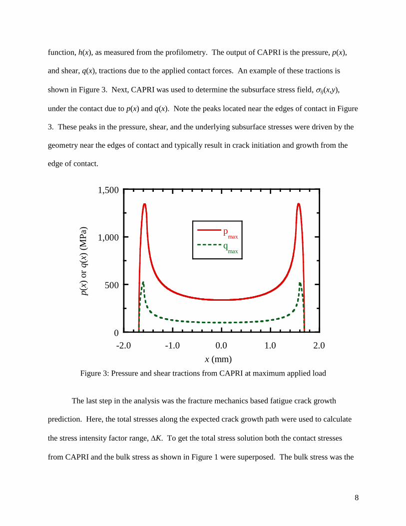
function, h(x), as measured from the profilometry. The output of CAPRI is the pressure, p(x),

and shear, q(x), tractions due to the applied contact forces. An example of these tractions is

shown in Figure 3. Next, CAPRI was used to determine the subsurface stress field, ij(x,y),

under the contact due to p(x) and q(x). Note the peaks located near the edges of contact in Figure

3. These peaks in the pressure, shear, and the underlying subsurface stresses were driven by the

geometry near the edges of contact and typically result in crack initiation and growth from the

edge of contact.

Figure 3: Pressure and shear tractions from CAPRI at maximum applied load

The last step in the analysis was the fracture mechanics based fatigue crack growth

prediction. Here, the total stresses along the expected crack growth path were used to calculate

the stress intensity factor range, K. To get the total stress solution both the contact stresses

from CAPRI and the bulk stress as shown in Figure 1 were superposed. The bulk stress was the

0

500

1,000

1,500

-2.0 -1.0 0.0 1.0 2.0

pmax

qmax

p(x

) or

q(x

) (M

Pa)

x (mm)

9

stress distribution induced in the component due to the remotely applied loading and the

geometry of the component. A procedure to obtain the bulk stress distribution for a dovetail

geometry was described by Golden and Calcaterra [12] which necessitated both the FEM model

and CAPRI results. Once the full subsurface stress distribution was known, the mode I stress

distribution could be extracted along the expected crack path at the edge of contact. Since this

stress distribution was nonlinear, weight function stress intensity factor solutions were applied

[16]. The crack propagation life was then integrated using a crack growth model of the form

KfdN

da (2)

where da/dN is the crack growth rate and the crack growth model f is discussed later.

Integration of life was performed using the Euler method with small step size starting from a

small initial fretting crack typically 25 mm in depth, until fracture. Crack growth properties

from previous testing on the same Ti-6Al-4V material used in the US Air Force High Cycle

Fatigue program [17] were applied.

3. Statistical Analysis

The random variables for the probabilistic fretting analysis performed in this study were

chosen from the key input variables of the deterministic analysis described above. These key

input variables included the initial crack size, the coefficient of friction, the slope that defines

the contact forces during partial slip, the crack growth law parameters, and the parameters

defining the shape of the pad profile. PDF’s were developed for each of these random variables

from measurements and test data available both from the dovetail fretting experiments and from

other fatigue and fatigue crack growth experiments. The details of the development of these

PDF’s are described below. A summary of the resulting PDF’s are shown in Table 1.

10

Initial crack size

The deterministic fretting fatigue life prediction analysis described above was a fracture

mechanics based crack propagation calculation. To perform this analysis an initial crack size

was required. Previous work [16] has shown that the initial fretting cracks tend to be shallow,

low aspect ratio (a/c) surface cracks that often appear to be several micro-cracks that have

coalesced. Here, a is the surface crack depth and c is the half surface length. Investigations of

naturally initiated cracks in smooth bar fatigue specimens in Ti-6Al-4V with the same

microstructure [18] have revealed that the cracks appear to initiate almost exclusively at primary

alpha grains at the surface of the specimen. These naturally initiated cracks in the primary alpha

grains form readily identifiable facets on the specimen fracture surface. Measurements of these

initial cracks were made in a prior study [18] on fatigue variability of Ti-6Al-4V, where repeated

tests were conducted at a few constant amplitude stress levels. The resulting distribution of

primary alpha grain facets was used here to represent the expected variability in initial fretting

crack depth. It is therefore assumed in this analysis that the naturally initiated fretting cracks

also form at the surface primary alpha grains, albeit at a different local stress state and surface

condition as in the prior study. Since it has been shown that typically multiple surface cracks

form and coalesce in fretting, a constant, low aspect ratio of a/c = 0.2 was used. The mean and

standard deviation of the measured naturally initiated crack sizes is listed in Table 1. It was

determined that a lognormal distribution was the best fit to the data.

Coefficient of friction and the partial slip slope

As described above and depicted in Figure 2, the coefficient of friction and the partial slip

slope of Q versus P were measured during each test. The accuracy of these measurements,

however, was limited to the accuracy of the strain gage instrumentation of the tests and the finite

11

element analysis that was used to convert fixture strain to applied load. Additionally, variability

in friction was expected from test to test. Both the measurement uncertainty and inherent

variability in the tests needed to be captured in the probabilistic model. To achieve this, data was

collected from twenty-three fretting tests all of which were conducted under similar loading

conditions. All tests were bare Ti-6Al-4V on Ti-6Al-4V contact (no coatings) and all were

loaded at R = 0.1. The measured values of friction coefficient and partial slip slope, , were

found to be correlated. The uncertainty in the expected values of friction and partial slip slope

along with their correlation was modeled using a multivariate normal distribution. In order to

avoid the possibility of an infinite slope, α, the value 1/α is used in the analysis procedure and

tabulated in Table 1.

Fatigue crack growth parameters

The crack growth rate curves used for crack propagation predictions were based on

fatigue crack growth tests previously conducted [17]. Four tests conducted at R = 0.1 and -1

from two different labs were fit to a bilinear crack growth model, where, da/dN is the crack

growth rate and K is the stress intensity factor range. These data are plotted in Figure 4. The

Walker model [19] was used to collapse the data from the different R values using an equation of

the form

𝑑𝑎 𝑑𝑁 = 𝐶1 ∆𝐾 1 − 𝑅 𝑚−1

𝑛1∆𝐾 < 𝑏

𝑑𝑎 𝑑𝑁 = 𝐶2 ∆𝐾 1 − 𝑅 𝑚−1 𝑛2

∆𝐾 > 𝑏 (3)

where b is the intersection point for regions 1 and 2, defined as

12

210110 loglog

nn

CCb

(4)

and the values of the Walker exponent m were determined in the previous program [9].

Different values were used for R < 0, m = 0.275, and R > 0, m = 0.72. The statistics of the curve

12

fit were modeled using a multivariate normal. The coefficients Ci and the exponents ni were

found to be correlated for each segment of the bilinear crack growth model. The mean, standard

deviation, and correlation coefficients are summarized in Table 1. The values of the model

parameters resulted units of MPam for K, and m/cycle for da/dN. The da/dN versus K

curves for one-hundred randomly generated realizations of Ci and ni were also plotted in Figure

4.

Figure XX: Plot of da/dN versus K data and 100 realizations of the bilinear model.

2 10 7010

-11

10-10

10-9

10-8

10-7

10-6

10-5

10-4

Keff

(MPa-m1/2

)

da/

dN

(m

/cy

cle)

2 10 7010

-10

10-9

10-8

10-7

10-6

10-5

10-4

10-3

Keff

(ksi-in1/2

)

da/

dN

(in

/cy

cle)

R = -1

R = -1

R = 0.1

R = 0.1

Realizations

13

Pad profile

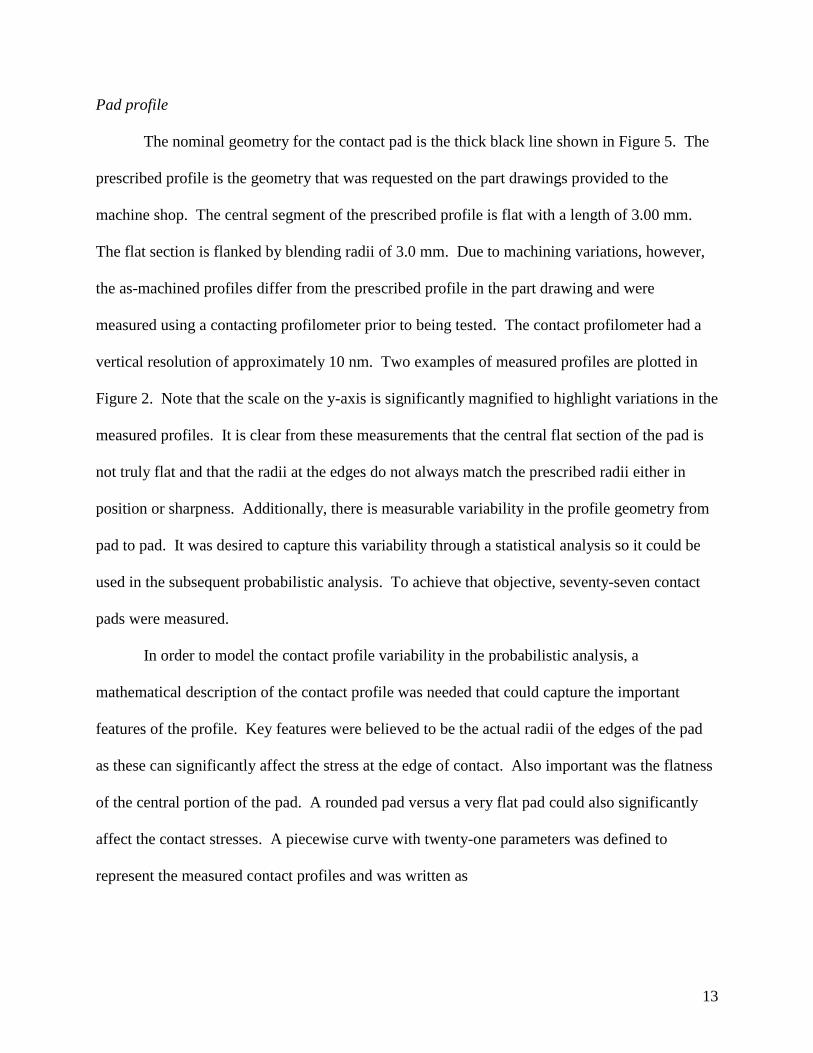
The nominal geometry for the contact pad is the thick black line shown in Figure 5. The

prescribed profile is the geometry that was requested on the part drawings provided to the

machine shop. The central segment of the prescribed profile is flat with a length of 3.00 mm.

The flat section is flanked by blending radii of 3.0 mm. Due to machining variations, however,

the as-machined profiles differ from the prescribed profile in the part drawing and were

measured using a contacting profilometer prior to being tested. The contact profilometer had a

vertical resolution of approximately 10 nm. Two examples of measured profiles are plotted in

Figure 2. Note that the scale on the y-axis is significantly magnified to highlight variations in the

measured profiles. It is clear from these measurements that the central flat section of the pad is

not truly flat and that the radii at the edges do not always match the prescribed radii either in

position or sharpness. Additionally, there is measurable variability in the profile geometry from

pad to pad. It was desired to capture this variability through a statistical analysis so it could be

used in the subsequent probabilistic analysis. To achieve that objective, seventy-seven contact

pads were measured.

In order to model the contact profile variability in the probabilistic analysis, a

mathematical description of the contact profile was needed that could capture the important

features of the profile. Key features were believed to be the actual radii of the edges of the pad

as these can significantly affect the stress at the edge of contact. Also important was the flatness

of the central portion of the pad. A rounded pad versus a very flat pad could also significantly

affect the contact stresses. A piecewise curve with twenty-one parameters was defined to

represent the measured contact profiles and was written as

14

𝑦 =

𝑘𝐿𝑥 + 𝑏𝐿 𝑥 < 𝑎1

𝑦0𝐿 + 𝑅𝐿 2 − 𝑥 − 𝑥0

𝐿 2 𝑎1 < 𝑥 < 𝑎2

𝑐0 + 𝑐1𝑥 + 𝑐2𝑥2 + 𝑐3𝑥

3 + 𝑐4𝑥4 + 𝑐5𝑥

5 + 𝑐6𝑥6 𝑎2 < 𝑥 < 𝑎3

𝑦0𝑅 + 𝑅𝑅 2 − 𝑥 − 𝑥0

𝑅 2 𝑎3 < 𝑥 < 𝑎4

𝑘𝑅𝑥 + 𝑏𝑅 𝑥 > 𝑎4

(5)

where x and y represent a Cartesian coordinate system with x along the profile and y is

the height of the profile. In the current problem the pad profile is pressed into a flate plate so the

function y is also the gap function h. The central segment of the profile (a2<x<a3) was

represented by a sixth order polynomial to allow the nominally flat section to have curvature.

Just outside the central section were two circular arcs to represent the radii at the edges of

contact. Just beyond the radii were flat taper sections. Through various constraints at x = a1 –

a4, the number of parameters was reduced from twenty-one to thirteen. These thirteen variables

kL, k

R, b

L, b

R, y0

L, x0

L, x0

R, R

L, R

R, c1, c2, c3, c4, c5, and c6 were determined from nonlinear

regression of each of the measured seventy-seven profiles. These variables were referred to as i,

where i ranged from 0 to 12. The remaining 8 variables in Equation 1 were functions of i as

defined by the constraints. The correlation coefficients for i are listed in Table 2, showing high

correlation among some of the variables. Finally, the results of the nonlinear regression from all

77 profiles were fit to a multivariate normal distribution. The mean and standard deviation of the

regression parameters are listed in Table 1. These variable values will result in a pad profile or

gap function, h, with units of µm. Three sample realizations of these fitted profiles are plotted in

Figure 6 along with the prescribed profile. The measured and the sampled profiles often differ

significantly from the prescribed profile, particularly near the edge of contact.

15

Figure 5: Prescribed and sample measured pad profiles.

Figure 6: Random realizations of the pad profile model compared to the prescribed profile.

-80

-60

-40

-20

0

20

-3000 -2000 -1000 0 1000 2000 3000

MeasuredMeasuredPrescribed

y (

m)

x (m)

-80

-60

-40

-20

0

20

-3000 -2000 -1000 0 1000 2000 3000

Prescribedsample 01sample 02sample 03

y (

m)

x (m)

16

Table 1: Summary of random variable statistics.

Random Variable No. Mean St. Dev. Distribution Type

Initial crack size, ai (µm) X1 15.1 8.48 Lognormal

Friction coefficient, ave X2 0.302 0.021 Correlated normal

23 = - 0.375 Partial slip slope, X3 1.96 0.120

Crack growth, log10(C1) X4 -14.6 0.486 Correlated normal

45 = -0.9973 Crack growth, n1 X5 7.19 0.715

Crack growth, log10(C2) X6 -11.8 0.157 Correlated normal

67 = -0.9751 Crack growth, n2 X7 3.81 0.146

Profile, 0 = kL X8 0.181 5.84x10

-3 Correlated normal

Profile, 1 = y0L X9 -2335 410 (see Table XX)

Profile, 2 = RL X10 2333 411

Profile, 3 = x0L X11 -1612 37.7

Profile, 4 = RR X12 2289 379

Profile, 5 = x0R X13 1620 35.4

Profile, 6 = kR X14 -0.183 4.96x10

-3

Profile, 7 = c1 X15 -2.00x10-4

6.20x10-4

Profile, 8 = c2 X16 -1.21x10-6

1.01x10-6

Profile, 9 = c3 X17 1.53x10-10

6.38x10-10

Profile, 10 = c4 X18 9.80x10-13

6.16x10-13

Profile, 11 = c5 X19 -3.77x10-17

1.87x10-16

Profile, 12 = c6 X20 -3.80x10-19

1.59x10-19

Table 2: Pad profile regression correlation coefficients

0 1 2 3 4 5 6 7 8 9 10 11 12

0 1 -0.079 0.078 -0.119 -0.051 0.184 -0.364 0.153 0.175 -0.107 -0.130 0.073 0.112

1 -0.079 1 -1.000 -0.921 -0.404 0.321 -0.122 0.093 -0.205 -0.203 0.281 0.275 -0.246

2 0.078 -1.000 1 0.921 0.404 -0.321 0.121 -0.092 0.207 0.203 -0.282 -0.275 0.247

3 -0.119 -0.921 0.921 1 0.325 -0.372 0.270 -0.019 0.104 0.136 -0.201 -0.247 0.219

4 -0.051 -0.404 0.404 0.325 1 -0.899 -0.204 -0.102 0.079 0.065 -0.116 0.002 0.123

5 0.184 0.321 -0.321 -0.372 -0.899 1 -0.033 0.010 -0.004 0.062 0.021 -0.147 -0.061

6 -0.364 -0.122 0.121 0.270 -0.204 -0.033 1 -0.095 -0.242 -0.017 0.142 0.078 -0.133

7 0.153 0.093 -0.092 -0.019 -0.102 0.010 -0.095 1 0.140 -0.876 -0.027 0.627 0.059

8 0.175 -0.205 0.207 0.104 0.079 -0.004 -0.242 0.140 1 -0.099 -0.869 0.057 0.765

9 -0.107 -0.203 0.203 0.136 0.065 0.062 -0.017 -0.876 -0.099 1 0.011 -0.915 -0.027

10 -0.130 0.281 -0.282 -0.201 -0.116 0.021 0.142 -0.027 -0.869 0.011 1 0.027 -0.944

11 0.073 0.275 -0.275 -0.247 0.002 -0.147 0.078 0.627 0.057 -0.915 0.027 1 -0.031

12 0.112 -0.246 0.247 0.219 0.123 -0.061 -0.133 0.059 0.765 -0.027 -0.944 -0.031 1

17

4. Probabilistic Analysis

Monte Carlo sampling was carried out to determine the moments (mean and standard

deviation) of the cycles-to-failure distribution. This procedure involved repeated generation of

realizations of the random variables and execution of the deterministic fretting fatigue algorithm

to determine cycles-to-failure. The deterministic fretting fatigue algorithm was simplified as

much as possible to minimize the computational time needed for each set of random variable

samples. All necessary calculations were performed using MATLAB since both CAPRI and the

crack growth calculation code were developed using MATLAB. This included calculation of the

contact forces using the method demonstrated by Gean and Farris [6], rather than modeling the

contact in a FEM analysis. The CAPRI run time was minimized by reducing the number of Fast

Fourier Transform terms to the minimum required and optimizing the solver parameters for this

problem. Finally, a linear fit of the bulk stresses as a function of the contact forces was created

from a series of FEM analyses, rather than using a new FEM analysis for each Monte Carlo run.

Eliminating the FEM analyses from the calculation of fretting fatigue life reduced the

computational time to approximately 1.2 s per simulation when running in parallel with 4

processors on an Intel Xeon quad core workstation. This made running the Monte Carlo analysis

with a significant number of samples possible. The ensemble of cycles to failure, Nf, results

were then analyzed to determine the mean and standard deviation. Sufficient samples were

executed to ensure high confidence in the computed moments.

Probabilistic sensitivities play an important role in determining insight into the dominant

factors governing a probabilistic analysis and provide information as to potentially effective

methods to improve the reliability. There are a number of methods in the literature such as

18

scatter plots [20], Pearson or Spearman correlation [21], regression methods [22], and the Score

function method [23], among others, that can provide useful information. The following is a

description of several methods used in the current work.

Scatter plots

Scatter plots are a two-dimensional point plot of the sample points versus the

corresponding response points. The sample realizations for each random variable (X) and the

corresponding results (Y) are plotted on separate axes. If a random variable is not important, no

pattern should be discernable, that is, the samples for X should mimic its marginal distribution.

Conversely, if a random variable is important, the pattern of realizations for X will be distinctly

non-random. Scatterplots are an inexpensive but qualitative method.

Regression and correlation

Linear regression (LR) methods are well known and widely available tools for assessing

variance contribution. LR approximates the relationship between response and the random

variables as

𝑦 𝑿 = 𝛽0 + 𝛽𝑖𝑓 𝑋𝑖 (6)

where f is an arbitrary function of the random variable Xi. In general, LR may contain

quadratic and interaction terms of any number of the variables, Xi.

The results from an LR model provide an easy mechanism to estimate the sensitivities of

the response (denoted Z) standard deviation (Z) to the standard deviation of the input parameters

(i), e.g., iZ , or of the response mean (µZ) to the mean of the input parameters (µi), e.g.,

iZ . This sensitivity in its nondimensionalized form

Z / i i /Z or

ZiiZ // provides an indication as to the relative importance of the random variables

and can be used to estimate design improvements.

19

One of the simplest linear regression models in terms of the original variables is

𝑍 = 𝐴0 + 𝐴1𝑋1 + ⋯ + 𝐴𝑛𝑋𝑛 (7)

In order to simplify the sensitivity equations derived below, Equation 1 can be rewritten

as the standardized model

n

nn

n

Z

XA

XA

S

ZZ

)(ˆ)(ˆ

1

111

(8)

where 𝑍 denotes the sampling mean of the response and 𝑆𝑍 represents the sampling

standard deviation of Z. Equation 2 can then be rewritten

𝑍 = 𝐴 1𝑋 1 + ⋯ + 𝐴 𝑛𝑋 𝑛 (9)

where the conversion between the original and standardized coefficients is

i

i

Zi AA ˆ

(10)

𝐴0 = 𝑍 − 𝐴1𝜇1 − ⋯− 𝐴𝑛𝜇𝑛 (11)

It is known that for a linear model of the form 𝑍 = 𝐴0 + 𝐴1𝑋1 + ⋯ + 𝐴𝑛𝑋𝑛 that the

expected value or mean value of Z can be written

n

i

ii XEAZE1

(12)

and the sensitivities or partial derivatives are simply

i

i

Z A

(13)

The variance of Z can be written as

n

i

n

j

jiijji AAZVar1 1

(14)

[24] and the sensitivities or partial derivatives are [25]

20

Z

i

Ai

Z

A jij j

j1

n

(15)

For independent variables (ij = 0) this reduces to

Z

i

i

Z

Ai

2 (16)

Note, based on Eq. (10), the sensitivity must be positive, whereas, based upon Eq. (9), the

sensitivity can be negative for negative correlation coefficients.

Rewriting the sensitivity in terms of standardized regression coefficients yields

Z

i

Z

i

ˆ A i

Z

Z

j

ˆ A jij j

j1

n

Z

i

ˆ A iˆ A jij

j1

n

(17)

Nondimensionalizing yields

Si Z

i

i

Z

i

Z

Z

i

ˆ A iˆ A jij

j1

n

ˆ A iˆ A jij

j1

n

(18)

For independent variables this reduces to

Si Z

i

i

Z

ˆ A i2 (19)

Finite Difference

The finite difference (FD) method [26] was used in this study to compute the

probabilistic sensitivities as a method of verifying other much more efficient methods such as

LR. FD is conducted by simply applying a small change in a random variable parameter (mean

or standard deviation) and then re-running the Monte-Carlo analysis to obtain a new response

distribution. The change in the modes of the response distribution divided by the change in the

random variable parameter, i.e. ∆𝜎𝑍 ∆𝜎𝑖 , gives an estimate of the probabilistic sensitivity,

𝜕𝜎𝑍 𝜕𝜎𝑖 . Calculation of the probabilistic sensitivities using FD can be very computationally

costly due to the large number of Monte Carlo simulations required. In the current problem there

21

are 20 random variables each with 2 parameters (mean and standard deviation) multiplied by a

sample size of 50,000 for each parameter results in 2 million simulations or approximately 1

month computation time. 50,000 was chosen as a necessary balance between accuracy and

computational cost. Unfortunately it is unlikely to be enough samples to achieve convergence in

the sensitivity estimate. In fact, additional simulations were performed to double the sample size

to 100,000 for the FD analysis of several variables of interest proving the estimates were either

converged (less than 5% change) or in some cases not converged. However, of those variables

of interest that were not converged changes in the estimates with sample size of 100,000 were

modest, i.e. 30% or less. A percent change in sensitivity estimates for many variable parameters

were not considered since the estimates were nearly zero.

5. Results and Discussion

Probabilistic Life Prediction

The probabilistic fretting fatigue life prediction tool was exercised at several

experimental load cases. Results were generated at the 5 applied loading conditions (Fmax = 18,

20, 22, 24, and 30 kN) used in the dovetail testing program. Lives were generated at each

loading condition initially using a sample size of 10,000 for the random variables initial crack

size, coefficient of friction, partial slip slope, crack growth curve, and the pad profile. These

results are plotted on lognormal probability paper in Figure 7 along with the experimental lives.

The solid lines are the distribution of the Monte Carlo predicted failure lives with the applied

highest load (30 kN) on the left and the lowest applied load (18 kN) on the right. The

experimental lives shown were as follows: 1,371,000, 10,000,000, and 693,000 cycles at 18 kN;

995,000 and 919,900 cycles at 20 kN; 249,900, 346,200, and 497,800 cycles at 22 kN; 164,000

cycles at 24 kN; and 105,000 cycles at 30 kN. These data were quite limited for an evaluation of

22

a probabilistic life prediction, however, they were still useful to ensure the predictions were near

the test results. The comparison in Figure 7 shows that at the higher loads the predictions were

closer than at the lower loads. Not surprisingly, all of the experimental results fall within the

scatter of the simulated results. At the lower applied loads, however, the test results seem to

deviate from the predictions by having longer lives. In fact, the longest life at 18 kN is over 10

million cycles (test was a run-out) which was at the 99% probability level of the prediction. If

the three 18 kN experiments do belong to the simulated failure life distribution there is less than

a 3% chance that this long life would occur in testing. This shows that the fracture mechanics

life prediction model is likely missing some of the physics of the problem. It supports the view

that crack nucleation or formation may be a significant portion of the life at lower stress levels,

even for a crack propagation model has an initial crack size at a microstructural scale.

23

Figure 7: Probability plot of experimental (points) and predicted (lines) lives at several applied

loads.

The results plotted in Figure 7 were generated with just 10,000 samples to minimize

processing time for each condition analyzed. Since the number of samples was relatively small,

an understanding of the variance in the estimates of mean and standard deviation of Nf was

important. Variance estimates of the mean and standard deviation of the distribution were

calculated at each of the applied forces and listed in Table 3. Since the distribution of Nf was

fairly lognormal, the modes of the distribution of the logarithm of Nf were calculated. The

estimates for mean of the log10 of Nf were then converted back to cycles. The columns showing

104

105

106

107

108

.001

.01

.1

1

510

2030

50

7080

9095

99

99.9

99.99

99.999

18 kN

20 kN

22 kN

24 kN

30 kN

Crack Growth Life, Nf (cycles)

Per

cen

t

24

the 95% confidence bounds of the mean were then converted back to cycles or the ratio of the

lower bound (LB) and upper bound (UB) to the mean cycle count. The coefficient of variance

(COV) was also calculated entirely in log units. Interestingly, the COV decreased with increased

applied loading, which was consistent with fatigue test results in Ti-6Al-4V [18] and it is

generally true in metallic aerospace materials that at higher stresses the variance in fatigue life

decreases. Also, in Table 3 the estimates of the mean and standard deviation of the distribution

were calculated for smaller and larger numbers of samples at Fmax = 22 kN. With more samples,

the confidence bounds shrink significantly as expected. In addition to quantifying the modes of

the distribution, PDF’s were fit to the distribution. Figure 8 is a plot of two PDF types fit to the

Nf results at Fmax = 22 kN. The solid line is a nonparametric kernel estimate of the PDF [26],

while the dashed curve was a lognormal fit to the Nf distribution. The differences in the PDF’s

showed that the distribution of failure lives was skewed toward longer lives and also had a higher

peak. This skewness toward longer lives in the tail can also be observed in Figure 7, and this

trend increased with smaller applied loads.

25

Figure 8: PDF estimates of Nf for 10,000 simulations at Fmax = 22 kN.

Table 3: Mean and coefficient of variation (c.o.v.) of the Monte Carlo analysis results including

the 95% upper bound (UB) and lower bound (LB) confidence limits

Mean of log10(Nf) COV of log10(Nf)

Fmax (kN) Sample

Size LB / Mean

Mean

(cycles) UB / Mean LB / COV COV UB / COV

18 kN 10,000 0.989 872,600 1.012 0.986 4.26% 1.012

20 kN 10,000 0.990 509,900 1.010 0.988 4.01% 1.012

22 kN 1000 0.973 328,400 1.028 0.960 3.54% 1.042

22 kN 10,000 0.991 326,200 1.009 0.987 3.72% 1.013

22 kN 500,000 0.999 324,300 1.001 0.998 3.70% 1.002

24 kN 10,000 0.992 225,400 1.008 0.989 3.51% 1.014

30 kN 10,000 0.993 95,400 1.007 0.988 3.24% 1.012

Sensitivity Results

Perhaps the simplest method to qualitatively determine sensitivity is through a scatter

plot. Figure 9 below shows the scatter plots that relate cycles-to-failure (y axis) with each

random variable (x axis) for 10,000 samples. The scatter plot for random variable X2 shows a

definite pattern. Correlation coefficients (Pearson or Spearman) for each variable relate to the

amount of variance in Y that can be apportioned to Xi. The results for Pearson correlation

0

1x10-6

2x10-6

3x10-6

4x10-6

105

106

KernelLognormal

PD

F

Nf (cycles)

26

coefficients, given in Table 4, indicate that variable X2 (coefficient of friction) is by far the

dominant variable, contributing 65% of the variance in Nf. It must be pointed out, however, that

the correlation coefficients are obtained without consideration for the simultaneous variations in

other random variables. A better estimate of variable importance can be determined using linear

regression, discussed below.

Figure 9: Scatter plots of the model output cycles to failure, Nf, versus the input random

variables, X1 through X20

In this research, an LR model of the form of Equation 6 was used, where X denotes a

vector of random variables,

y represents the cycles-to-failure and the ’s are coefficients that are

fit to the analytical results. Table 5 shows the results of a “best model” fit using a specified

number of variables. For example, using only 2 variables, the combination of X2 and X16 account

for the largest percentage of the variance in Nf. Note, once X2 is included in the model, adding

X16 adds 17 percent to the R2 sum, however, the R

2 value using the Pearson correlation

Nf Nf Nf Nf Nf

Nf Nf Nf Nf Nf

Nf Nf Nf Nf Nf

Nf Nf Nf Nf Nf

X1 X2 X3 X4 X5

X6 X7 X8 X9 X10

X11 X12 X13 X14 X15

X16 X17 X18 X19 X20

27

coefficient for X2 without considering any other random variables is 25%. From the results, one

can see quickly the diminished returns offered after the first few random variables. For example,

if only 5 random variables are used in an LR model, this model would account for 85% out of a

possible 91% of the output variance. It is somewhat surprising that a simple linear model with

respect to the random variables can account for such a large percentage of the output variance.

Table 4: R2 values for the random variables

Variable R2

X1 0.024

X2 0.645

X3 0.093

X4 0.001

X5 0.002

X6 0.006

X7 0.002

X8 0.002

X9 0.004

X10 0.004

X11 0.003

X12 0.005

X13 0.017

X14 0.008

X15 0.007

X16 0.063

X17 0.013

X18 0.020

X19 0.020

X20 0.038

28

Table 5: Best model linear regression results

N R2 C(p) Random Variables in Model

1 0.645 28,370 X2

2 0.713 21,020 X2 X16

3 0.754 16,620 X2 X9 X10

4 0.824 9000 X2 X16 X18 X20

5 0.846 6660 X1 X2 X16 X18 X20

6 0.855 5710 X1 X2 X13 X16 X18 X20

7 0.874 3640 X1 X2 X6 X7 X16 X18 X20

8 0.883 2690 X1 X2 X6 X7 X13 X16 X18 X20

9 0.898 1060 X1 X2 X6 X7 X16 X17 X18 X19 X20

10 0.901 720 X1 X2 X6 X7 X13 X16 X17 X18 X19 X20

Table 6 shows the results using LR considering natural groupings of random variables.

The variables were partitioned into 4 groups: (X1 - initial crack size, X2-X3 coefficient of friction

– partial slip slope, X4-X7 crack growth parameters, X8-X20 geometry profile). The results

indicate that group 2 is dominant, followed by the geometry profile. Surprisingly, the

traditionally dominant random variables in fatigue, crack growth rate and initial crack size are

not significant in terms of their contribution to the output variance, e. g., these parameters could

be modeled deterministically.

Table 6: Linear regression group analysis showing the effect of each random variable group on

the model R2

Group RV Added # RV Model

R2

R2 C(p) F value

1 X2, X3 2 0.645 0.645 28,370 9080

2 X8 – X20 15 0.210 0.855 5710 1110

3 X4 – X7 19 0.030 0.885 2420 660

4 X1 20 0.022 0.908 20 2410

Next, we wish to quantify the probabilistic sensitivities, particularly the sensitivity of the

standard deviation of the response (life) to the random variable parameters mean, 𝜕𝜎𝑍 𝜕𝜇𝑖 , and

standard deviation, 𝜕𝜎𝑍 𝜕𝜎𝑖 . Figure 10 is a bar chart of the normalized sensitivity of the

standard deviation of the cycles to failure, Nf, response, denoted Z, to the standard deviation of

the random variables, Xi, simply denoted by i in Equation 19. Results from the finite difference

29

analysis and linear regression show very good agreement. The analysis shows that the standard

deviation of the response is by far most sensitive to the standard deviation of the coefficient of

friction (X2) and to several parameters of the flat section of the contact profile (X16 - X20). The

slope of the first segment of the bilinear crack growth law (X5) and the intercept of the second

segment (X6) also have relatively high sensitivities. Also notable is the sensitivity of the initial

crack size (X1) is quite small. The sensitivities of these variables is essential to understand when

evaluating which variables are most important to the process being analyzed. One must also

consider, however, the likelihood that the estimates of these random variable parameters will

change due to additional or better quality data, or that these parameters can change through an

alteration to the system, i.e. machining tolerances or addition of coatings.

Figure 10: Comparison of Si for FD and LR.

Figure 10 helped to identify that the standard deviation of X16, X18, and X20 were

parameters with a relatively high sensitivity. It is not intuitive, however, how these variables

-0.4

-0.2

0.0

0.2

0.4

0.6

0.8

1.0

1 2 3 4 5 6 7 8 9 10 11 12 13 14 15 16 17 18 19 20

No

rmal

ized

Sen

siti

vit

y, S

i

Random Variable, Xi

Finite Difference

Linear Regression

30

affect the pad profile. Further analysis of the profile has shown that the flatness of the “flat”

section (a2 < x < a3) of the pad profile is strongly affected by the values of these variables. Here,

flatness is defined as the peak to peak height difference in y. A probabilistic fretting analysis

was performed the pad profile being the only group of random variables. The remaining

variables were deterministic. The results showed a significant correlation between log10 𝑁𝑓 and

X16, X18, and X20 of 0.35 to 0.55, however, the correlation between log10 𝑁𝑓 and flatness was

0.77. Figure 11 is a scatter plot showing this relationship.

Figure 11: Scatter plot of fatigue crack growth life versus profile flatness showing far stronger

correlation than with any of the random variables.

6. Conclusions

A new probabilistic fretting analysis was developed to investigate the relative importance

of typical fretting input variables on the predicted failure lives. Several random variable inputs

were identified and PDF’s were quantified using laboratory data. Monte Carlo sampling of the

105

106

1 10

Nf (

cycl

es)

Flatness, ymax

- ymin

(m)

31

input PDF’s was performed and a deterministic analysis was repeatedly run using the sampled

inputs to obtain a distribution of predicted fretting lives. The results were compared to

experimental fretting fatigue tests and the predictions were much closer at higher stresses than at

lower stress possibly due to substantial crack nucleation lives at the lower stresses. The results

showed that considerable scatter in fretting lives can be expected based on variability in the

material properties, contact profiles, coefficient of friction, and contact force response.

Interestingly, the dominant variables in terms of contribution to the cycles-to-failure variance

were the coefficient of friction and several terms within the geometry profile; whereas, the

traditionally dominant variables in fatigue crack growth analyses, initial crack size and crack

growth, were not as significant.

Acknowledgements

The authors would like to thank Prof. Farris and his students at Purdue University for

providing the CAPRI software used in this study. This work was partially supported by the Air

Force Research Laboratory, Materials and Manufacturing Directorate through subcontract

USAF-5212-STI-SC-0021 from General Dynamics Information Technology to the University of

Texas at San Antonio.

References

[1] Dang Van K, “Macro–micro approach in high-cycle multiaxial fatigue,” In: D.L.

McDowell and R. Ellis, Editors, Advances in Multiaxial Fatigue, ASTM STP 1191,

Philadelphia (1993), pp. 120–130.

[2] Lykins CD. Mall S. Jain V. An Evaluation of Parameters for Predicting Fretting Fatigue

Crack Initiation. Int J Fatigue. 2000;22:703-716.

[3] Fridrici V, Fouvry S, Kapsa P, Perruchaut P, “Prediction of Cracking in Ti–6Al–4V Alloy

Under Fretting-Wear: Use of the SWT Criterion,” Wear 2005, 259, pp 300-308.

[4] Murthy, “Fretting Fatigue of Ti-6Al-4V Subjected to Blade/Disk Contact Loading,”

Developments in Fracture Mechanics for the New Century, 50th Anniversary of Japan

Society of Materials Science, Osaka, Japan, pp. 41-48, 2001.

32

[5] Rooke DP, Jones, DA. Stress Intensity Factors in Fretting Fatigue. J Strain Analysis

1979;14:1-6.

[6] Hattori T, Nakamura M, Sakata H, Watanabe T. Fretting Fatigue Analysis Using Fracture

Mechanics. JSME Int J 1988;31:100-107.

[7] Chan KS, Yi-Der Lee, Davidson DD, Hudak SJ, Jr. A Fracture Mechanics Approach to

High Cycle Fretting Fatigue Based on the Worst Case Fret Concept. Int J Fracture

2001;112:299-330.

[8] Kumari S, Farris, TN, “Statistical Analysis of Effect of Contact Surface Profile on Fretting

Fatigue Life for Ti-6Al-4V,” 47th

AIAA/ASME/ASCE/AHS/ASC Structures, Structural

Dynamics, and Materials Conference, AIAA 2006.

[9] Zhang R, Mahadevan S, “Probabilistic Prediction of Fretting Fatigue Crack Nucleation

Life of Riveted Lap Joints,” 41st AIAA/ASME/ASCE/AHS/ASC Structures, Structural

Dynamics, and Materials Conference, AIAA-2000-1645, 2000.

[10] Chevalier L, Cloupet S, Soize C, “Probabilistic Model for Random Uncertainties in Steady

State Rolling Contact,” Wear 2005, 258, pp 1543-1554.

[11] Golden PJ, Nicholas T, “The Effect of Angle on Dovetail Fretting Experiments in Ti-6Al-

4V,” Fatigue and Fracture of Engineering Materials and Structures, 28, 2005, pp. 1169-

1175.

[12] Golden PJ, Calcaterra. A Fracture Mechanics Life Prediction Methodology Applied to

Dovetail Fretting. Tribology International, Vol. 39, 2006, pp.1172-80.

[13] Gean, M.C., Farris, T.N., “Mechanics Modeling of Firtree Dovetail Contacts,” 49th

AIAA/ASME/ASCE/AHS/ASC Structures, Structural Dynamics, and Materials

Conference, AIAA 2008-2176, 2008.

[14] Chan KS, Enright MP, Moody JP, Golden PJ, Chandra R, Pentz AC, “Residual Stress

Profiles for Mitigating Fretting Fatigue in Gas Turbine Engine Disks,” Int J Fatigue, Vol.

X, 2009, pp. XX-XX.

[15] McVeigh PA, Harish G, Farris TN, Szolwinski MP. Modeling interfacial conditions in

nominally flat contacts for application to fretting fatigue of turbine engine components.

International Journal of Fatigue , Vol. 21, 1999; pp. S157–65.

[16] Golden, P.J., Grandt, A.F., Jr., “Fracture mechanics based fretting fatigue life predictions

in Ti–6Al–4V,” Engineering Fracture Mechanics, Vol. 71, 2004, pp. 2229-2243.

[17] Gallagher JP, et al. AFRL-ML-TR-2001-4159, Improved High-Cycle Fatigue (HCF) Life

Prediction, Wright-Patterson Air Force Base, OH, 2001.

[18] Golden, P.J., John, R., Porter, W.J., III, “Variability in Room Temperature Fatigue Life of

Alpha+Beta Processed Ti-6Al-4V,” International Journal of Fatigue, 2009,

doi:10.1016/j.ijfatigue.2009.01.005.

[19] Walker, K., “The Effect of Stress Ratio During Crack Propagation and Fatigue for 2024-

T3 and 7075-T6 Aluminium,” Effects of Environment and Complex Load History on

Fatigue Life (10th edn), ASTM STP 462, American Society for Testing of Materials, PA,

1970, pp. 1–14.

33

[20] J.P.C.Kleijnen, and J.C. Helton, “Statistical Analyses of Scatterplots to Identify Important

Factors in Large-scale Simulation, Review and comparison of techniques,” Reliability

Engineering and System Safety, 65,1999, pp.147-185

[21] D.M. Hamby, “A Review of Techniques for Parameter Sensitivity Analysis of

Environmental Models,” Environmental Monitoring and Assessment 1994, 32, pp 135-154

[22] N.R. Draper and H. Smith, Applied Regression Analysis, 3rd Ed., Wiley-Interscience,

1998

[23] Rubinstein R.Y. and Shapiro, A. Discrete Event Systems, Sensitivity Analysis And

Stochastic Optimization By The Score Function Method. J. Wiley & Sons, Chichester,

England, 1993.

[24] Ang H-S.A, Tang WH, Probability Concepts in Engineering, Wiley, USA, 2007.

[25] H.R. Millwater, “Universal Properties of Kernel Functions for Probabilistic Sensitivity

Analysis,” Probabilistic Engineering Mechanics, Vol 24, 2009, 89–99

[26] B.W. Silverman, Density Estimation for Statistics and Data Analysis, Chapman &

Hall/CRC, Baco Raton, FL, 1998