AFOSR PROGRAM REVIEWJUNE 5-7, 2003PRINCETON, NJ

DATA HIDING IN TIME-FREQUENCY DISTRIBUTION OF

IMAGESBijan Mobasseri

ECE DepartmentVillanova UniversityVillanova, PA 19085

2

Outline

• Data hiding definition and modalities

• Motivation for using TF distributions

• Wigner distribution

• Watermarking model

• Embedding and detection

• Capacity

• Future work

3

Data hiding requirements

• Data hiding must meet at least the following three conditions:– Transparency; no visible impact on the cover

signal– Robustness; Survive “friendly fire”: filtering,

compression, cropping but break under attacks – Security; hidden data should not be easily

removed or replaced

4

Data hiding modalities

• Watermarking– Message itself is not secret: owner identification, copyright

protection, fingerprinting– Transparency, robustness and security still apply.– Embedding capacity not a major issue– In authentication applications, watermark must be content-

dependent, secure but somewhat brittle

• Steganography– Used as a covert channel, the message is secret and its

very presence within the host data must not be detectable

5

Information hiding as a game

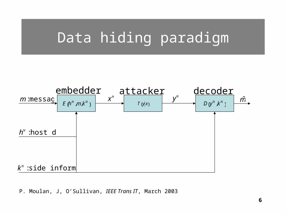
• Information hiding has been stated as a game between two cooperative players (embedder and decoder) and an opponent (attacker)

• The first party tries to maximize a payoff function and the opponent tries to minimize it (Moulin, O’Sullivan)

6

Data hiding paradigm

€

E h N ,m,k N( )

€

T y x( )

€

D yN ,k N( )

embedder attacker decoder

€

xN

€

yN

€

ˆ m

€

m : message

€

hN : host data

€

k N : side information

P. Moulan, J, O’Sullivan, IEEE Trans IT, March 2003

7

New domain

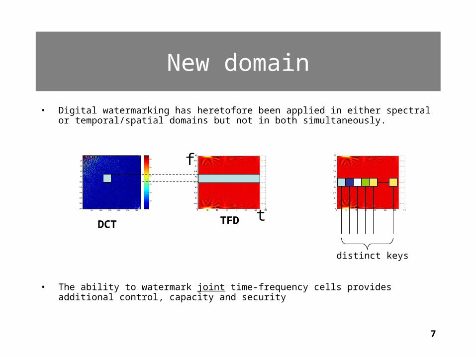
• Digital watermarking has heretofore been applied in either spectral or temporal/spatial domains but not in both simultaneously.

• The ability to watermark joint time-frequency cells provides additional control, capacity and security

50 100 150 200 250 300

20

40

60

80

100

120

140

160

180

200

10

20

30

40

50

60

DCT TFD t

f

distinct keys

8

Time-varying data hiding

t

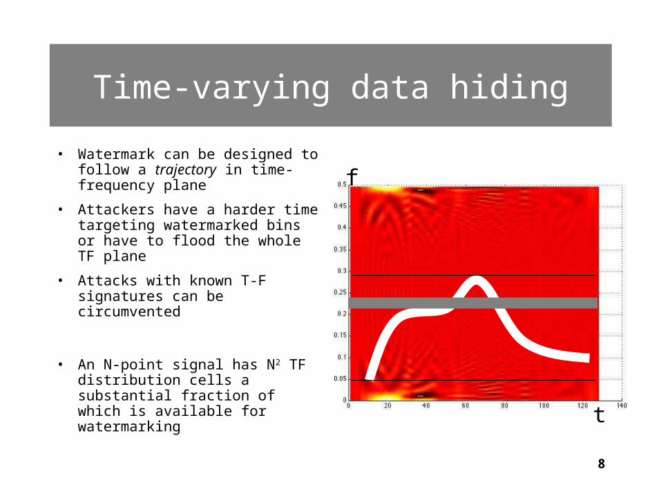
f• Watermark can be designed

to follow a trajectory in time-frequency plane

• Attackers have a harder time targeting watermarked bins or have to flood the whole TF plane

• Attacks with known T-F signatures can be circumvented

• An N-point signal has N2 TF distribution cells a substantial fraction of which is available for watermarking

9

Previous work

S. Stankovic, I. Djurovic, I. Pitas, “Watermarking in the space/spatial-frequency domain using two-dimensional Radon-Wigner distribution, “IEEE Transaction on Image Processing, vol. 10, no. 4, pp.650-658, April 2001.

• They add a sinusoidal pattern to the image in a way that is only detectable in time-frequency domain. It is presented as a watermarking algorithm

• Our approach hides data in the transform domain instead

10

Generating TFD:Wigner Distribution

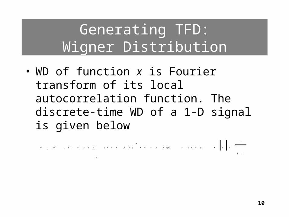
• WD of function x is Fourier transform of its local autocorrelation function. The discrete-time WD of a 1-D signal is given below

Wx

nT , f( ) = 2 T x n + m( )

m

∑ x

*

n − m( ) (exp − j 4 π fmT ), f ≤

1

4 T

11

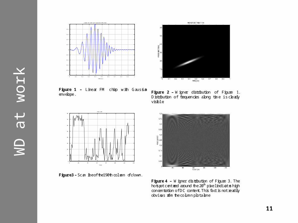
WD

at

work 0 0.1 0.2 0.3 0.4 0.5 0.6 0.7 0.8 0.9 1

-1

-0.8

-0.6

-0.4

-0.2

0

0.2

0.4

0.6

0.8

1

TIME(sec)

LINEAR FM CHIRP WITH GAUSSIAN AMPLITUDE

Figure 1 – Linear FM chirp with Gaussianenvelope. Figure 2 – Wigner distribution of Figure 1.

Distribution of frequencies along time is clearlyvisible.

0 20 40 60 80 100 120 140

0

10

20

30

40

50

60

70

80

SCAN LINE

PIXEL

Figure 3 – Scan line of the190th column of clown.

Figure 4 – Wigner distribution of Figure 3. Thehotspot centered around the 20th pixel indicates highconcentration of DC content. This fact is not readilyobvious from the column plot alone

12

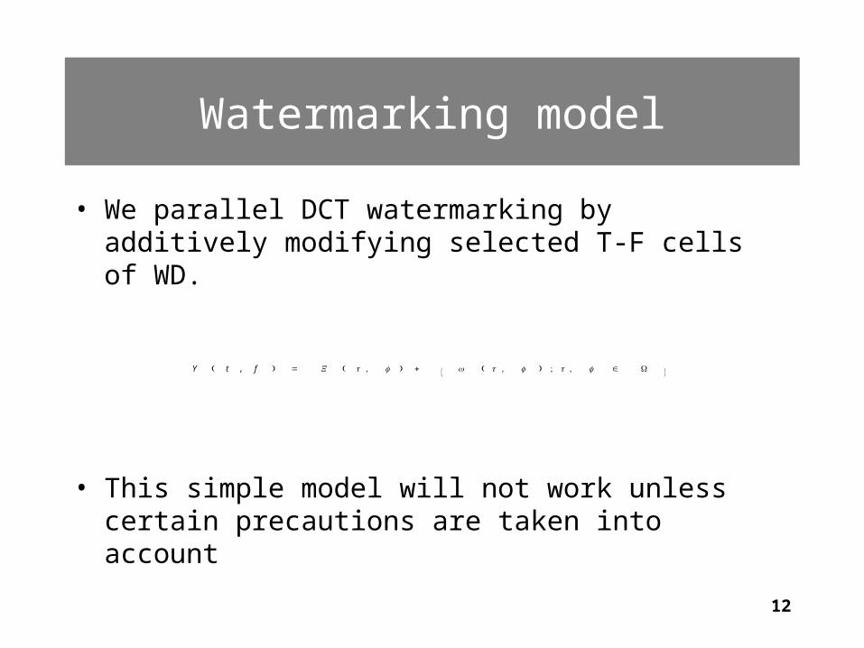
Watermarking model

• We parallel DCT watermarking by additively modifying selected T-F cells of WD.

• This simple model will not work unless certain precautions are taken into account

Y t , f( ) = X t , f( ) + w t , f( ) ; t , f ∈ Ω{ }

13

The Inverse Wigner

• Not every two dimensional function is an allowed time-frequency representation

• It is possible that no signal may be found that has the given TFD

• This is a synthesis problem and can be stated as follows

Given a target (watermarked) WD Y, find the corresponding signal x whose Wigner distribution is closest to Y in some sense

14

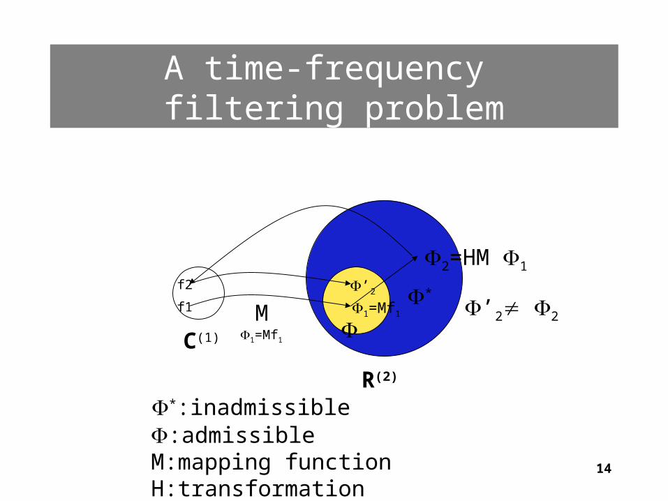
A time-frequency filtering problem

C(1)

R(2)

f1

f2

1=Mf1

’2

M*

*:inadmissible

:admissibleM:mapping functionH:transformation

2=HM 1

’2 2

1=Mf1

15

Solutions

• There are a number of solutions to this problem.

For DTWD:

V. Kumar et al, “Discrete Wigner synthesis,” Signal Processing, vol. 11, pp. 277-304, 1986.

For DWD:

S. Nelatury, B. Mobasseri,” Synthesis of discrete-time discrete-frequency Wigner Distribution “ IEEE Signal Processing Letters, in press.

16

Exam

ple

: ti

me-f

requ

ency

filt

eri

ng

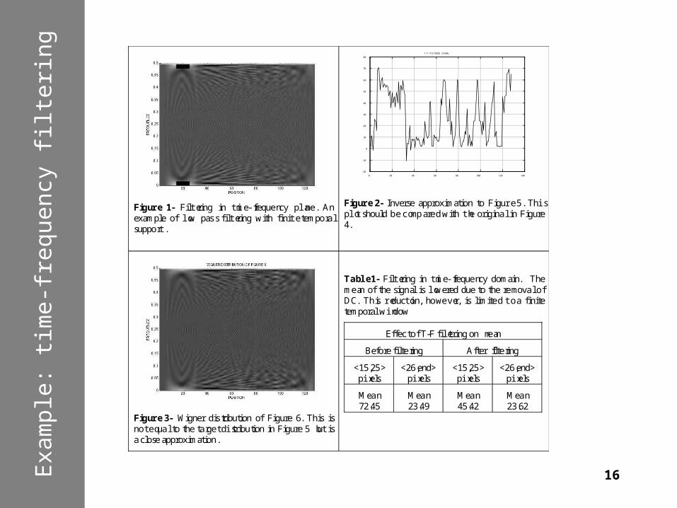
Figure 1- Filtering in time-frequency plane. Anexample of low pass filtering with finite temporalsupport.

0 20 40 60 80 100 120 140

-20

-10

0

10

20

30

40

50

60

70

80

T-F FILTERED SIGNAL

Figure 2- Inverse approximation to Figure 5. Thisplot should be compared with the original in Figure4.

Figure 3- W igner distribution of Figure 6. This isnot equal to the target distribution in Figure 5 but isa close approximation.

Table 1- Filtering in time-frequency domain. Themean of the signal is lowered due to the removal ofDC. This reduction, however, is limited to a finitetemporal window

Effect of T-F filtering on mean

Before filtering After filtering

<15,25>pixels

<26,end>pixels

<15,25>pixels

<26,end>pixels

Mean72.45

Mean23.49

Mean45.42

Mean23.62

17

2D Wigner

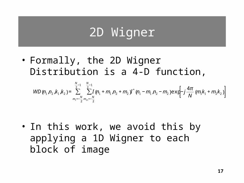
• Formally, the 2D Wigner Distribution is a 4-D function,

• In this work, we avoid this by applying a 1D Wigner to each block of image

€

WD n1,n2,k1,k2( ) = I n1 + m1,n2 + m2( )m21 =−

N

2

N

2−1

∑m1 =−

N

2

N

2−1

∑ I * n1 − m1,n2 − m2( )exp − j4π

Nm1k1 + m2k2( )

⎡ ⎣ ⎢

⎤ ⎦ ⎥

18

1D Wigner distribution of 2D block

• Let define an NxN image block

• Define an “equivalent” linear array then do a 1D Wigner on it €

X,xij , i, j( )∈ N{ }

€

rX

€

º º º º

º º º º

º º º º

º º º º

€

º º º º

º º º º

º º º º

º º º º

€

º º º º

º º º º

º º º º

º º º º

Column-wise zigzag random

19

Picking the order

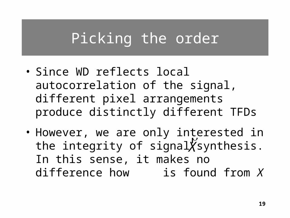
• Since WD reflects local autocorrelation of the signal, different pixel arrangements produce distinctly different TFDs

• However, we are only interested in the integrity of signal synthesis. In this sense, it makes no difference how is found from X

€

rX

20

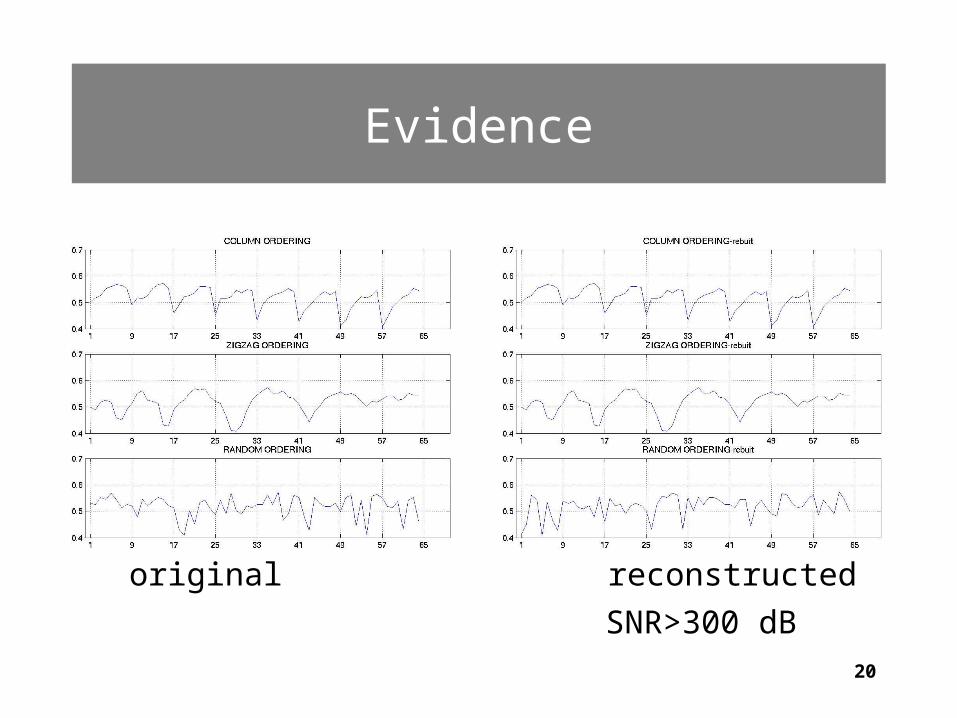
Evidence

SNR>300 dB

original reconstructed

21

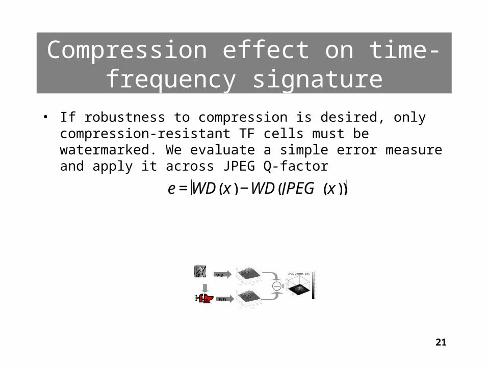
Compression effect on time-frequency signature

• If robustness to compression is desired, only compression-resistant TF cells must be watermarked. We evaluate a simple error measure and apply it across JPEG Q-factor

€

e=WD x( )−WD JPEG x( )( )

22

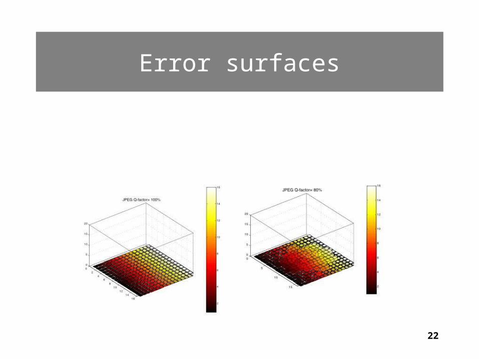
Error surfaces

23

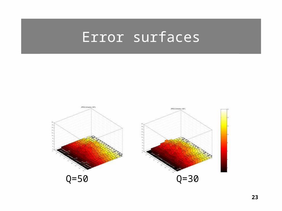
Error surfaces

Q=30Q=50

24

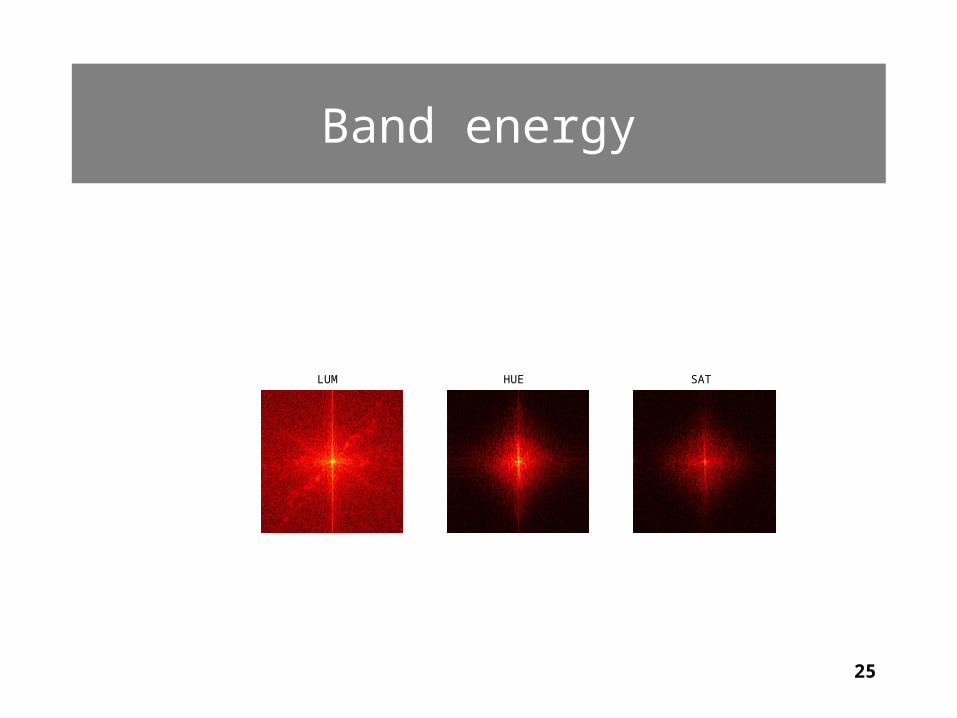
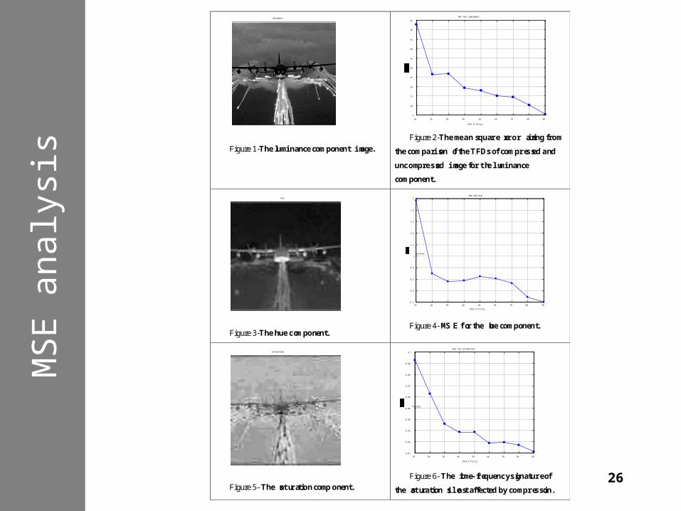
Which component to watermark?

• JPEG follows YUV(luma-hue-saturation) color model.

• We have found that the TF signature of saturation band is most robust to compression

LUMINANCEHUE SATURATION

25

Band energy

LUM HUE SAT

26

LUMINANCE

Figure 1-The luminance component image.

10 20 30 40 50 60 70 80 90

5

10

15

20

25

30

35

40

45

50

55

MSE FOR LUMINANCE

JPEG Q-factor

Figure 2-The mean square error arising from

the comparison of the TFDs of compressed and

uncompressed image for the luminance

component.

HUE

Figure 3-The hue component.

10 20 30 40 50 60 70 80 90

0.2

0.4

0.6

0.8

1

1.2

1.4

1.6

1.8

2

MSE FOR HUE

JPEG Q-factor

MSE TextEnd

Figure 4- MSE for the hue component.

SATURATION

Figure 5- The saturation component.

10 20 30 40 50 60 70 80 90

0.01

0.02

0.03

0.04

0.05

0.06

0.07

0.08

0.09

0.1

MSE FOR SATURATION

JPEG Q-factor

MSE TextEnd

Figure 6- The time-frequency signature of

the saturation is least affected by compression.

MSE a

naly

sis

27

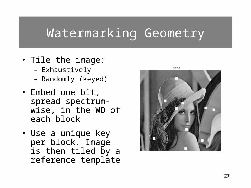
Watermarking Geometry

• Tile the image:– Exhaustively– Randomly (keyed)

• Embed one bit, spread spectrum-wise, in the WD of each block

• Use a unique key per block. Image is then tiled by a reference template

ORIGINAL

28

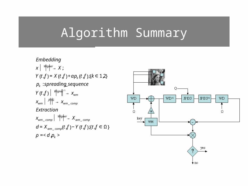
Algorithm Summary

€

Embedding

x Wigner ⏐ → ⏐ ⏐ X;

Y t, f( ) = X t, f( ) +αpk t, f( ); k ∈1,2{ }

pk : spreading_ sequence

Y t, f( ) Wigner −1

⏐ → ⏐ ⏐ ⏐ xwm

xwmJPEG ⏐ → ⏐ ⏐ xwm _ comp

Extraction

xwm _ compWigner ⏐ → ⏐ ⏐ Xwm _ comp

d = Xwm _ comp t, f( ) − Y t, f( ); t, f ∈Ω{ }

ρ =< d ,pk >

29

Watermark detection

• Watermark is detected based on the following hypothesis testing– Ho: – H1:

• Rejecting the null hypothesis, when it is true, amounts to the probability of false alarm(picture is incorrectly decided to carry watermark)

€

ρ ≠0

€

ρ =0

30

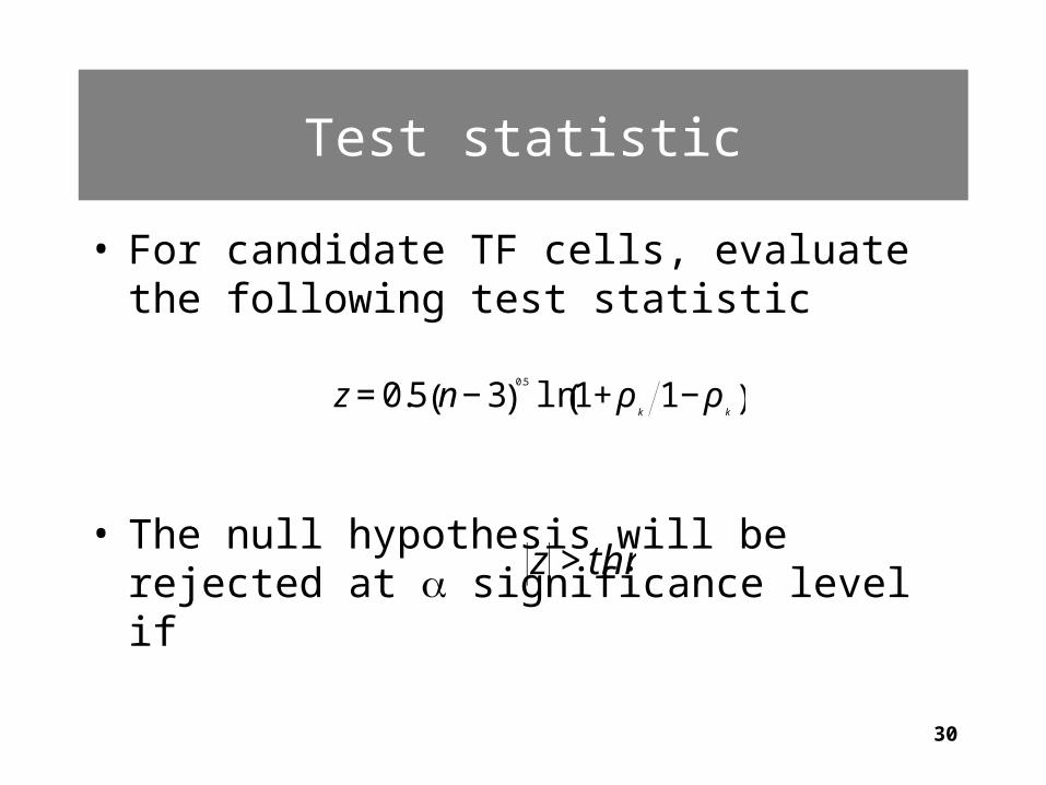
Test statistic

• For candidate TF cells, evaluate the following test statistic

• The null hypothesis will be rejected at significance level if

€

z = 0.5 n − 3( )0.5

ln 1+ ρk

1− ρk

( )

€

z > thr

31

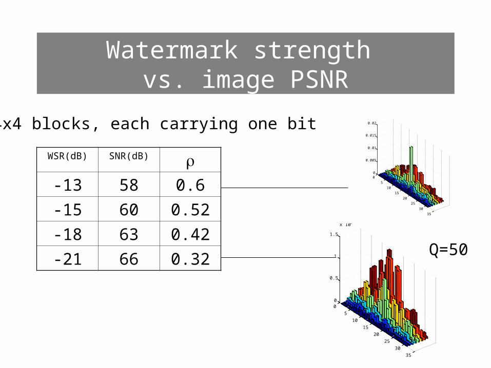
Watermark strength vs. image PSNR

WSR(dB) SNR(dB) ρ-13 58 0.6

-15 60 0.52

-18 63 0.42

-21 66 0.32

0

5

10

15

20

25

30

35

0

0.5

1

1.5

x 10-3

0

5

10

15

20

25

30

35

0

0.005

0.01

0.015

0.024x4 blocks, each carrying one bit

Q=50

32

Resu

lts

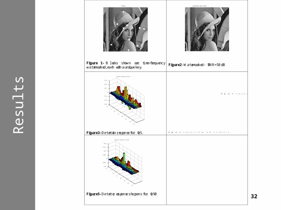
ORIGINAL

Figure 1- B locks shown are time-frequencywatermarked, each with a unique key.

WATERMARKED-LUMINA CHANNEL

Figure 2- Watermarked- PSNR=58 dB

0

5

10

15

20

25

30

35

-0.03

-0.02

-0.01

0

0.01

0.02

0.03

Detector response for Q=5

Figure 3- Detection response for Q=5.

QuickTime™ and aPhoto - JPEG decompressorare needed to see this picture.

Fi gu re 4 - F i g u r e 1 7 co mp re sse d w i t h Q = 5

0

5

10

15

20

25

30

35

-0.01

-0.005

0

0.005

0.01

0.015

0.02

Detector response for Q=50

Figure 5- Detector response sharpens for Q=50

QuickTime™ and aPhoto - JPEG decompressorare needed to see this picture.

Fi gu re 6 - F i g u r e 1 7 co mpr e ss ed w i th Q= 5 0

33

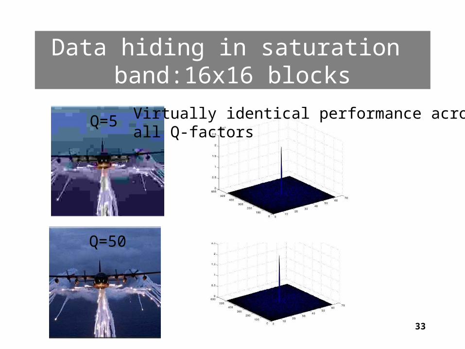
Data hiding in saturation band:16x16 blocks

Q=5

Q=50

Virtually identical performance acrossall Q-factors

34

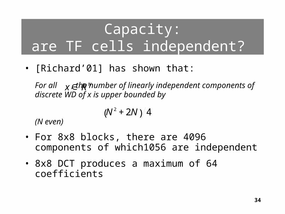
Capacity:are TF cells independent?

• [Richard’01] has shown that:

For all , the number of linearly independent components of discrete WD of x is upper bounded by

(N even)

• For 8x8 blocks, there are 4096 components of which1056 are independent

• 8x8 DCT produces a maximum of 64 coefficients

€

x∈RN

€

N2 +2N( ) 4

35

Payload numbers

• Capacity=N2/block_size

• Larger block size provides bigger PG and watermark survival at lower Q

• In lena(2562), we can embed 4096 bits using 4x4 blocks at WSR= -13dB

• Reliable detection is possible down to Q=25

36

Conclusions and future work

• A new transform domain for sata hiding is introduced

• It features high capacity, low probability of intercept and low JPEG Q-factor operation

• Need work on blind detection

• Robustness to geometric transformations

• Capacity and Steganalysis benchmarking

THE END