1Affine Maps in 3D

Figure 1.1.

Affine maps in 3D: fighter jets twisting and turning through 3D space.

This chapters wraps up the basic geometry tools. A�ne maps

in 3D are a primary tool for modeling and computer graphics.

Figure 1.1 illustrates the use of various a�ne maps. This chap-

ter goes a little farther than just a�ne maps by introducing

2 A�ne Maps in 3D

projective maps { the maps used to create realistic 3D images.

1.1 Affine Maps

Linear maps relate vectors to vectors. A�ne maps relate points

to points. A 3D a�ne map is written just as a 2D one, namely

as

x0 = p+A(x� o): (1.1)

In general we will assume that the origin of x's coordinate sys-

tem has three zero coordinates, and drop the o term:

x0 = p+Ax: (1.2)

Sketch 1.1 gives an example. Recall, the column vectors of A

are the vectors a1;a2;a3. The point p tells us where to move

the origin of the [e1; e2; e3]-system; again, the real action of an

a�ne map is captured by the matrix. Thus by studying matrix

actions, or linear maps, we will learn more about a�ne maps.

ForSketch,seebook

Sketch 1.

An affine map in 3D.

We now list some of the important properties of 3D a�ne

maps. They are straightforward generalizations of the 2D cases,

and so we just give a brief listing.

1. A�ne maps leave ratios invariant (see Sketch 1).

ForSketch,seebook

Sketch 2.

Affine maps leave ratios invari-

ant.

2. A�ne maps take parallel planes to parallel planes (see Figure

1.2).

3. A�ne maps take intersecting planes to intersecting planes.

In particular, the intersection line of the mapped planes is

the map of the original intersection line.

4. A�ne maps leave barycentric combinations invariant. If

x = c1p1 + c2p2 + c3p3 + c4p4;

where c1+ c2+ c3+ c4 = 1, then after an a�ne map we have

x0 = c1p

0

1+ c2p

0

2+ c3p

0

3+ c4p

0

4:

For example, the centroid of a tetrahedron will be mapped

to the centroid of the mapped tetrahedron (see Sketch 4).

ForSketch,seebook

Sketch 3.

The centroid is mapped to the

centroid.

1.2 Translations 3

Figure 1.2.

Parallel planes get mapped to parallel planes via an affine map.

Most 3D maps do not o�er much over their 2D counterparts

{ but some do. We will go through all of them in detail now.

1.2 Translations

A translation is simply (1.2) with A = I, the 3 � 3 identity

matrix:

I =

241 0 0

0 1 0

0 0 1

35 ;

that is

x0 = p+ Ix:

Thus the new [a1;a2;a3]�system has its coordinate axes par-

allel to the [e1; e2; e3]-system. The term Ix = x needs to be

interpreted as a vector in the [e1; e2; e3]-system for this to make

4 A�ne Maps in 3D

sense! Figure 1.3 shows an example of repeated 3D translations.

Figure 1.3.

Translations in 3D: three translated teapots.

Just as in 2D, a translation is a rigid body motion. The

volume of an object is not changed.

1.3 Mapping Tetrahedra

A 3D a�ne map is determined by four point pairs pi ! p0

i for

i = 1; 2; 3; 4. In other words, an a�ne map is determined by a

tetrahedron and its image. What is the image of an arbitrary

point x under this a�ne map?

A�ne maps leave barycentric combinations unchanged. This

will be the key to �nding x0, the image of x. If we can write x

in the form

x = u1p1 + u2p2 + u3p3 + u4p4; (1.3)

1.3 Mapping Tetrahedra 5

then we know that the image has the same relationship with

the p0i:

x0 = u1p

0

1 + u2p0

2 + u3p0

3 + u4p0

4: (1.4)

So all we need to do is �nd the ui! These are called the barycen-

tric coordinates of x with respect to the pi, quite in analogy to

the triangle case (Section ??).

We observe that (1.3) is short for three individual coordinate

equations. Together with the barycentric combination condi-

tion

u1 + u2 + u3 + u4 = 1;

we have four equations for the four unknowns u1; : : : ; u4, which

we can solve by consulting Chapter ??.

EXAMPLE 1.1

Let the original tetrahedron be given by the four points pi

240

0

0

35 ;

241

0

0

35 ;

240

1

0

35 ;

240

0

1

35 :

Let's assume we want to map this tetrahedron to the four points

p0

i 240

0

0

35 ;

24�10

0

35 ;

240

�10

35 ;

240

0

�1

35 :

This is a pretty straightforward map if you consult Sketch 1.3.

ForSketch,seebook

Sketch 4.

An example tetrahedron map.Let's see where the point x =

241

1

1

35 ends up! First, we �nd

that 241

1

1

35 = �2

240

0

0

35+

241

0

0

35+

240

1

0

35+

240

0

1

35 ;

i.e., the barycentric coordinates of x with respect to the orig-

inal pi are (�2; 1; 1; 1). Note how they sum to one! Now it is

6 A�ne Maps in 3D

simple to compute the image of x; compute x0 using the same

barycentric coordinates with respect to the p0i:

x0 = �2

240

0

0

35+

24�10

0

35+

240

�10

35+

240

0

�1

35 =

24�1�1�1

35 :

A di�erent approach would be to �nd the 3�3 matrix A and

point p which describe the a�ne map. Construct a coordinate

system from the pi tetrahedron. One way to do this is to choose

p1 as the origin1 and the three axes are de�ned as pi � p1 for

i = 2; 3; 4. The coordinate system of the p0i tetrahedron must

be based on the same indices. Once we have de�ned A and p

then we will be able to map x by this map:

x0 = A[x� p1] + p

0

1

Thus the point p = p0

1. In order to determine A, let's write

down some known relationships. Referring to Sketch 1.3, we

know

A[p2 � p1] = p0

2� p

0

1;

A[p3 � p1] = p0

3� p

0

1;

A[p4 � p1] = p0

4� p

0

1;

which may be written matrix form as

A�p2 � p1 p3 � p1 p4 � p1

�=�p0

2� p

0

1p0

3� p

0

1p0

4� p

0

1

�:

(1.5)

Thus

A =�p0

2� p

0

1p0

3� p

0

1p0

4� p

0

1

� �p2 � p1 p3 � p1 p4 � p1

��1

;

(1.6)

and A is de�ned.

ForSketch,seebook

Sketch 5.

The relationship between tetra-

hedra.

1Any of the four pi would do, so for the sake of concreteness, we pick

the �rst one.

1.4 Projections 7

EXAMPLE 1.2

Revisiting the previous example, we now want to construct

the matrix A. By selecting p1 as the origin for the pi tetrahe-

dron coordinate system there is no translation; p1 is the origin

in the [e1; e2; e3]-system and p0

1= p1. We now compute A. (A

is the product matrix in the bottom right position):

1 0 0

0 1 0

0 0 1

�1 0 0

0 �1 0

0 0 �1

�1 0 0

0 �1 0

0 0 �1

In order to compute x0, we have

x0 =

24�1 0 0

0 �1 0

0 0 �1

35241

1

1

35 =

24�1�1�1

35 :

This is the same result as in the previous example.

1.4 Projections

Take any object made of wires outside; let the sun shine on

it, and you can observe a shadow. This shadow is the parallel

projection of your object onto a plane. Everything we draw is

a projection of necessity { paper is 2D, after all, whereas most

interesting objects are 3D. Figure 1.4 gives an example. Also

see Figure ??.

Projections reduce dimensionality; as basic linear maps, we

encountered them in Sections ?? and ??. As a�ne maps, they

map 3D points onto a plane. In most cases, we are interested

in the case of these planes being the coordinate planes. All we

have to do then is set one of the point's coordinates to zero.

8 A�ne Maps in 3D

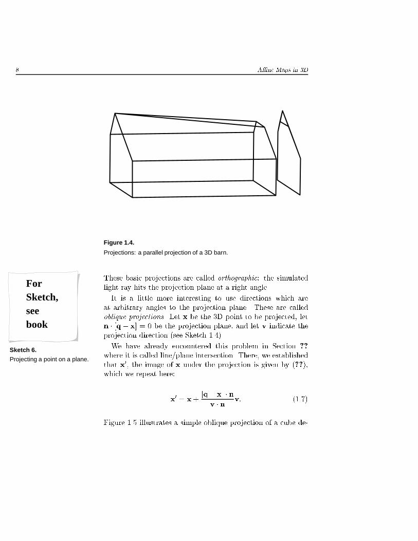
Figure 1.4.

Projections: a parallel projection of a 3D barn.

These basic projections are called orthographic: the simulated

light ray hits the projection plane at a right angle.

It is a little more interesting to use directions which are

at arbitrary angles to the projection plane. These are called

oblique projections. Let x be the 3D point to be projected, let

n � [q � x] = 0 be the projection plane, and let v indicate the

projection direction (see Sketch 1.4).

ForSketch,seebook

Sketch 6.

Projecting a point on a plane.

We have already encountered this problem in Section ??

where it is called line/plane intersection. There, we established

that x0, the image of x under the projection is given by (??),

which we repeat here:

x0 = x+

[q� x] � nv � n

v: (1.7)

Figure 1.5 illustrates a simple oblique projection of a cube de-

1.4 Projections 9

�ned over [�1; 1] in each coordinate with

n =

241

0

0

35 q =

242

0

0

35 v =

241=p2

1=p2

0

35 :

Figure 1.6 creates a projection plane that is not one of the

coordinate planes; speci�cally,

n =

241=p3

1=p3

1=p3

35 q =

244

0

0

35 v =

241=p3

1=p3

1=p3

35 :

Finally, Figure 1.7 creates a general oblique projection with

n =

241=p3

1=p3

1=p3

35 q =

244

0

0

35 v =

241=p2

1=p2

0

35 :

Revisiting the helix, Figure 1.8 is a projection with the same n

and v as in the previous �gure.

How do we write this as an a�ne map? Without much e�ort,

we �nd

x0 = x�

n � xv � n

v+q � nv � n

v:

We know that we may write dot products in matrix form (see

Section ??):

x0 = x�

nTx

v � nv+

q � nv � n

v:

Next, we observe that

[nT � x]v = v[nTx]:

Since matrix multiplication is associative (see Section ??), we

also have

v[nTx] = [vnT]x;

and thus

x0 = [I �

vnT

v � n]x+

q � nv � n

v: (1.8)

10 A�ne Maps in 3D

Figure 1.5.

Projections: a cube projected in a coordinate plane with an oblique angle.

This is of the form x0 = Ax+ p and hence is an a�ne map!2

The term vnT might appear odd, yet it is well-de�ned. It is

a 3� 3 matrix, as in the following example.

EXAMPLE 1.3

1 3 3

1

2

0

1 3 3

2 6 6

0 0 0

All rows of this matrix are multiples of each other; so are

2Technically we should add the origin in order for p to be a point.

1.4 Projections 11

Figure 1.6.

Projections: a cube projected in an arbitrary plane with a right angle.

all columns. Matrices which are generated like this are called

dyadic; their rank is one.

EXAMPLE 1.4

Let a plane be given by x1 + x2 + x3 � 1 = 0, a point x and

a direction v by

x =

243

2

4

35 ; v =

240

0

�1

35 :

If we project x along v onto the plane, what is x0? First, we

need the plane's normalized normal. Calling it n, we have

n =1p3

241

1

1

35 :

12 A�ne Maps in 3D

Figure 1.7.

Projections: a cube projected in an arbitrary plane with an oblique angle.

Now choose a point q in the plane. Let's choose q =

241

0

0

35 for

simplicity. Now we are ready to calculate the quantities in (1.8):

v � n = �1=p3;

vnT

1=p3=

1 1 1

0

0

�1

0 0 0

0 0 0

�1 �1 �1

,

q � nv � n

v =

240

0

1

35 :

1.4 Projections 13

Figure 1.8.

Projections: a helix projected in an arbitrary plane with an oblique angle.

Putting all the pieces together:

x0 = [I �

240 0 0

0 0 0

�1 �1 �1

35243

2

4

35+

240

0

1

35 =

243

2

�4

35

Just to double check, enter x0 into the plane equation

3 + 3� 4� 1 = 0;

and we see that243

2

4

35 =

243

2

�4

35+ 8

240

0

1

35 ;

which together verify that this is the correct point.

Sketch 1.4 should convince you that this is indeed the correct

answer.

ForSketch,seebook

Sketch 7.

A projection example.

14 A�ne Maps in 3D

Which of the two possibilities, (1.7) or the a�ne map (1.8)

should you use? Clearly (1.7) is more straightforward and less

involved. Yet in some computer graphics or CAD system en-

vironments, it may be desirable to have all maps in a uni�ed

format, i.e., Ax+ p.

1.5 Homogeneous Coordinates and Perspective Maps

There is a way to condense the form x0 = Ax + p of an a�ne

map into just one matrix multiplication

x0 = Mx: (1.9)

This is achieved by setting

M =

2664

a1;1 a1;2 a1;3 p1a2;1 a2;2 a2;3 p2a3;1 a3;2 a3;3 p30 0 0 1

3775

and

x =

2664

x1x2x31

3775 ; x

0 =

2664

x01

x02

x03

1

3775 :

The 4D point x is called the homogeneous form of the a�ne

point x. You should verify for yourself that (1.9) is indeed the

same a�ne map as before!

The homogeneous form is more general than just adding a

fourth coordinate x4 = 1 to a point. If, perhaps as the result of

some computation, the fourth coordinate does not equal one,

one gets from the homogeneous point x to its a�ne counterpart

x by dividing through by x4. Thus one a�ne point has in�nitely

many homogeneous representations!

EXAMPLE 1.5

1.5 Homogeneous Coordinates and Perspective Maps 15

(The symbol t should be read \corresponds to".)

241

�13

35 t

2664

10

�1030

10

3775 t

2664

�22

�6�2

3775 :

This example shows two homogeneous representations of one

a�ne point.

Using the homogeneous matrix form of (1.9), the matrix M

for the point into a plane projection from (1.8) becomes24v � n 0 0

0 v � n 0

0 0 v � n

35� vn

T (q � n)v

0 0 0 v � n

.

Here, the element m4;4 = v � n. Thus x4 = v � n, and we

will have to divide x's coordinates by x4 in order to obtain the

corresponding a�ne point.

A simple change in our equations will lead us from parallel

projections onto a plane to perspective projections. Instead of

using a constant direction v for all projections, now the direc-

tion depends on the point x. More precisely, let it be the line

from x to the origin of our coordinate system. Then, as shown

in Sketch 1.5, v = �x, and (1.7) becomes

x0 = x+

[q� x] � nx � n

x;

which quickly simpli�es to

x0 =

q � nx � n

x: (1.10)

In homogeneous form, this is described by the following matrix

M :I[q � n] o

0 0 0 x � n.

ForSketch,seebook

Sketch 8.

Perspective projection.

16 A�ne Maps in 3D

Perspective projections are not a�ne maps anymore! To see

this, a simple example will su�ce.

EXAMPLE 1.6

Take the plane x3 = 1; let q =

240

0

1

35 be a point on the plane.

Now q � n = 1 and x � n = x3, resulting in the map

x0 =

1

x3x:

Take the three points

x1 =

242

0

4

35 ; x2 =

243

�13

35 ; x3 =

244

�22

35 :

This example is illustrated in Sketch 1.5. Note that x2 =1

2x1+

1

2x3, i.e., x2 is the midpoint of x1 and x3.

Their images are

x0

1=

241=2

0

1

35 ; x

0

2=

24

1

�1=31

35 ; x

0

3=

242

�11

35 :

The perspective map destroyed the midpoint relation! For now

x0

2= 2

3x0

1+ 1

3x0

3.

Thus the ratio of three points is changed by perspective maps.

As a consequence, two parallel lines will not be mapped to par-

allel lines. Because of this e�ect, perspective maps are a good

model for how we perceive 3D space around us. Parallel lines

do seemingly intersect in a distance, and are thus not perceived

as being parallel! Figure 1.9 is a parallel projection and Figure

1.10 illustrates the same geometry with a perspective projec-

tion. Notice in the perspective image, the sides of the bounding

cube that move into the page are no longer parallel.

1.6 Exercises 17

Figure 1.9.

Parallel projection: A 3D helix and two orthographic projections on the left

and bottom walls of the bounding cube – not visible due to the orthographic

projection used for the whole scene.

The study of perspective goes back to the fourteenth century

{ before that, artists simply could not draw realistic 3D images.

One of the foremost researchers in the area of perspective maps

was A. D�urer; see Figure 1.11 for one of his experiments.3

1.6 Exercises

We'll use four points

x1 =

241

0

0

35 ; x2 =

240

1

0

35 ; x3 =

240

0

�1

35 ; x4 =

240

0

1

35

3From The Complete Woodcuts of Albrecht D�urer, edited by W. Durth,

Dover Publications Inc., New York, 1963. A website with material on

D�urer: http://www.bilkent.edu.tr/wm/paint/auth/durer/.

18 A�ne Maps in 3D

Figure 1.10.

Perspective projection: A 3D helix and two orthographic projections on the

left and bottom walls of the bounding cube – visible due to the perspective

projection used for the whole scene.

and four points

y1 =

24�10

0

35 ; y2 =

240

�10

35 ; y3 =

240

0

�1

35 ; y4 =

240

0

1

35 ;

and also the plane through q with normal n:

q =

241

0

0

35 ; n =

1

5

243

0

4

35 :

1. Using a direction

v =1

4

242

0

2

35 ;

1.6 Exercises 19

Figure 1.11.

Perspective maps: an experiment by A. Durer.

what are the images of the xi when projected onto the plane

with this direction?

2. Using the same v as in the previous problem, what are the

images of the yi?

3. What are the images of the xi when projected onto the plane

by a perspective projection through the origin?

4. What are the images of the yi when projected onto the plane

by a perspective projection through the origin?

5. Compute the centroid c of the xi and then the centroid c0 of

their perspective images (previous Exercise). Is c0 the image

of c under the perspective map?

6. An a�ne map xi ! yi; i = 1; 2; 3; 4 is uniquely de�ned.

What is it?

20 A�ne Maps in 3D

7. What is the image of

p =

241

1

1

35

under the map from the previous problem? Use two ways to

compute it.

8. What are the geometric properties of the a�ne map from

the last two problems?

9. We claimed that (1.8) reduces to (1.10). This necessitates

that

[I �vn

T

n � v]x = 0:

Show that this is indeed true.