aethalometer instrument handbook - arm climate … aethalometer instrument handbook aj sedlacek,...

DOE/SC-ARM-TR-156

Aethalometer™ Instrument Handbook AJ Sedlacek April 2016

DISCLAIMER

This report was prepared as an account of work sponsored by the U.S. Government. Neither the United States nor any agency thereof, nor any of their employees, makes any warranty, express or implied, or assumes any legal liability or responsibility for the accuracy, completeness, or usefulness of any information, apparatus, product, or process disclosed, or represents that its use would not infringe privately owned rights. Reference herein to any specific commercial product, process, or service by trade name, trademark, manufacturer, or otherwise, does not necessarily constitute or imply its endorsement, recommendation, or favoring by the U.S. Government or any agency thereof. The views and opinions of authors expressed herein do not necessarily state or reflect those of the U.S. Government or any agency thereof.

DOE/SC-ARM-TR-156

Aethalometer™ Instrument Handbook AJ Sedlacek, Brookhaven National Laboratory April 2016 Work supported by the U.S. Department of Energy, Office of Science, Office of Biological and Environmental Research

AJ Sedlacek, April 2016, DOE/SC-ARM-TR-156

iii

Acronyms and Abbreviations

A aerosol collecting spot area of filter, [cm²] AC alternating current ARM Atmospheric Radiation Measurement Climate Research Facility ASCII American Standard Code for Information Exchange ATN attenuation B surface loading of black carbon on filter, [g/cm2] BC black carbon Cm centimeter CSV comma-separated values DC direct current DOE U.S. Department of Energy EC elemental carbon ER extended range F flow rate of air through filter, liters per minute HS high sensitivity Hz Hertz LED light-emitting diode LPM liters per minute m3 square meter mbar millibars MB megabytes mm millimeter ȝJ microgram ng nanogram nm nanometers PCMCIA Personal Computer Memory Card International Association PPM parts per million RAM random access memory RB reference beam detector output with lamps on RZ reference beam detector zero output with lamps off SB sensing beam detector output with lamps on SG specific attenuation cross section for the aerosol black carbon deposit on filter

using optical components of instrument [m²/gram] SLPM standard liters per minute SZ sensing beam detector zero offset output with lamps off T sampling time-base period, minutes


iv

UV ultraviolet V volts


v

Contents

Acronyms and Abbreviations ...................................................................................................................... iii 1.0 Instrument Title .................................................................................................................................... 1 2.0 Mentor Contact Information ................................................................................................................. 1 3.0 Vendor/Developer Contact Information ............................................................................................... 1 4.0 Instrument Description ......................................................................................................................... 1 5.0 Measurements Taken ............................................................................................................................ 2 6.0 Links to Definitions and Relevant Information .................................................................................... 3

6.1 Data Object Description ............................................................................................................... 3 6.1.1 Data Modes Overview ....................................................................................................... 3 6.1.2 Digital Data Output Port (mode used by the Mobile Aerosol Observing System) ........... 3

6.2 Data Plots ..................................................................................................................................... 4 6.3 Instrument Mentor Monthly Summary......................................................................................... 4 6.4 Calibration Database .................................................................................................................... 5

7.0 Technical Specifications ....................................................................................................................... 5 7.1 Units ............................................................................................................................................. 5 7.2 Range ............................................................................................................................................ 5 7.3 Accuracy ...................................................................................................................................... 5 7.4 Repeatability ................................................................................................................................ 6 7.5 Sensitivity ..................................................................................................................................... 6 7.6 Uncertainty ................................................................................................................................... 6 7.7 Input Voltage ................................................................................................................................ 6 7.8 Output Values ............................................................................................................................... 6 7.9 Instrument System Functional Diagram ....................................................................................... 7

8.0 Instrument/Measurement Theory.......................................................................................................... 7 8.1 The Optical Attenuation Method .................................................................................................. 8 8.2 The Aethalometer Algorithm ..................................................................................................... 10

9.0 Setup and Operation of Instrument ..................................................................................................... 12 9.1 Assumption: The Hardware Is Already Setup in the Mobile Aerosol Observing System

Container .................................................................................................................................... 12 9.2 Quick Setup Summary Guide ..................................................................................................... 12 9.3 Filter Tape Installation ............................................................................................................... 13 9.4 Install New Tape – Operator Actions – Rack-Mount Models .................................................... 13 9.5 Install New Tape – Software Procedure Prompts ...................................................................... 14

10.0 Software .............................................................................................................................................. 15 10.1 Use of the Keypad ...................................................................................................................... 16 10.2 Menu Tree .................................................................................................................................. 16 10.3 Main System Menu upon Power-Up .......................................................................................... 20


vi

10.4 Data File Format......................................................................................................................... 20 10.4.1 Format Types................................................................................................................... 20 10.4.2 Data Continuation ........................................................................................................... 21 10.4.3 “Message” File Contents ................................................................................................. 22

10.5 Screen Display: Normal Operation ............................................................................................ 22 11.0 Calibration .......................................................................................................................................... 23 12.0 Maintenance........................................................................................................................................ 25

12.1 Disassembly and Cleaning ......................................................................................................... 25 12.2 Replacement of Bypass Filter Cartridge .................................................................................... 26 12.3 Flow Audit: Flowrate Error Scaling ........................................................................................... 27

13.0 Safety 28 14.0 Citable References .............................................................................................................................. 28

Figures

1. Exterior view of Aethalometer. ............................................................................................................. 2 2. Interior view of Aethalometer. .............................................................................................................. 2 3. Dual-wavelength and multi-wavelength Aethalometer data taken on different days in an

urban location but subject to local wood-fire smoke on both occasions. .............................................. 4 4. Cross section of optical analysis head. ................................................................................................. 7 5. Flow diagram of Aethalometer operation. ............................................................................................ 8


1

1.0 Instrument Title

Aethalometer™

2.0 Mentor Contact Information

Dr. Tony Hansen Magee Scientific Company Berkeley, CA Telephone: +1 (510) 845-2801 Fax: +1 (510) 845-7137 E-mail: [email protected]

3.0 Vendor/Developer Contact Information

Magee Scientific Corporation 1916A M. L. King Jr. Way Berkeley CA 94704 USA Telephone: +1 (510) 845-2801 Fax: +1 (510) 845-7137 http://www.mageesci.com/ Instrument manual available at http://www.mageesci.com/images/stories/docs/Aethalometer_book_2005.07.03.pdf

4.0 Instrument Description

The Aethalometer is an instrument that provides a real-time readout of the concentration of “Black” or “Elemental” carbon aerosol particles (BC or E) in an air stream (see Figure 1 and Figure 2). It is a self-contained instrument that measures the rate of change of optical transmission through a spot on a filter where aerosol is being continuously collected and uses the information to calculate the concentration of optically absorbing material in the sampled air stream. The instrument measures the transmitted light intensities through the “sensing” portion of the filter, on which the aerosol spot is being collected, and a “reference” portion of the filter as a check on the stability of the optical source. A mass flowmeter monitors the sample air flow rate. The data from these three measurements is used to determine the mean BC content of the air stream.

The Aethalometer performs the optical analysis and data readout “on the spot.” The results are available immediately to the user without having to wait to analyze a sample at a laboratory. It is a self-contained, automatic instrument, and it requires no consumable materials, no gas cylinders, and no operator attention. The only calibration required is a periodic check of the air flowmeter response.

mailto:[email protected]

http://www.mageesci.com/

http://www.mageesci.com/images/stories/docs/Aethalometer_book_2005.07.03.pdf


2

Figure 1. Exterior view of Aethalometer.

Figure 2. Interior view of Aethalometer.

5.0 Measurements Taken

The Aethalometer measures optical attenuation to determine BC aerosol concentrations expressed in terms of grams per cubic meter.


3

6.0 Links to Definitions and Relevant Information

6.1 Data Object Description

6.1.1 Data Modes Overview

The measurement data are made available to the user in the following four different modes:

1. Display screen. The most recent BC concentration is displayed in units of Pg BC/m³.

2. BC files and MF files on disk. The measurement data are written in the BC files, and the instrument operation messages are logged in the MF files. If the Overwrite Old Data parameter is set to YES, old data is overwritten by new data when the disk is almost full. The structure of the BC and MF files is described in the Operate Procedure section.

3. Analog output voltage on rear-panel terminals. A digital-analog converter connected to the rear-panel terminals provides a voltage that can represent the value of the BC concentration. The proportionality between this output voltage (0 to +5 V) on the terminals and the BC concentration is set by programming the Output Scale Factor. The default value of this scaling factor is set to 1 mV = 10 ng/m³ BC (i.e., 1 = 10 µg/m³ BC), but can be changed in the Change Settings menu. The analog voltage output is forced to -5 V to indicate “data not valid” during tape advance, instrument initialization, etc. This connection also can be configured as an alarm to turn ON or OFF according to the BC concentration. See the following section for more details.

4. Digital data at COM port (mode used by the Mobile Aerosol Observing System). If the COM Mode parameter is set to “DATALINE,” the COM port will produce a single line of data once per time-base period that is a replica of the data line written to disk. The transmission parameters (baud, parity, etc.) are set by the COM settings menu.

6.1.2 Digital Data Output Port (mode used by the Mobile Aerosol Observing System)

The rear panel of the instrument is fitted with a nine-pin socket that provides a standard COM port output for digital data reporting. The only connections that are used are pins 2, 3, and 7 (i.e., the ground). This port may be connected to a data recorder such as a commercial digital data logger or a computer running a ‘terminal’ program. The transmitted data line is an exact replica of the data line written to diskette, as described in Section 6.1.1.4 above.

The Aethalometer outputs data once per time base period, at the end of the period when the data line is written to diskette. Data are not stored internally, and cannot be retrieved upon command from an external interrogator. Thus, any data capture system must be set for continuous reception. It is not possible to connect a device to the Aethalometer’s COM port and download data upon command.

For connection to a standard PC computer, a ‘null-modem’ cable must be used. This cable interchanges the connections to pins 2 and 3.


4

6.2 Data Plots

Dual- and multi-wavelength Aethalometer data taken on different days in an urban location but subject to local wood-fire smoke on both occasions are shown in Figure 3. The “urban ambient” data show the typical large variations in EC concentration that occur as a result of the interplay between source emission strength and meteorological dispersion. However, this location was also impacted by “local” smoke from residential fireplaces burning wood. The lack of spectral differentiation during the day is clear, as is the signature of ultraviolet (UV)-absorbing organics during the evening.

Figure 3. Dual-wavelength (top) and multi-wavelength Aethalometer data taken on different days in an

urban location but subject to local wood-fire smoke on both occasions.

6.3 Instrument Mentor Monthly Summary

On a monthly basis, Aethalometer data are checked for quality assurance/quality control during data reduction by the mentor.


5

6.4 Calibration Database

The Aethalometer is an absolute measurement based on sample flow, spot size, and optical attenuation. The sample flow is checked annually (see Section 12.0).

7.0 Technical Specifications

x Measurement specifications

– Measurement range: 0 to 500 Pg/m3

– Resolution: 0.1 µg/m3 (dependent on dynamic range setting)

– Time Response: 5 minutes

– Baseline drift: automatically corrected by use of a reference filter.

x Physical specifications:

– Dimensions: 19 inches wide, 11 inches high, 12 inches deep

– Weight: <40 pounds.

x Power requirements: 85 to 250 VAC/50 to 400 Hz

x Power consumption: <55 W

7.1 Units

Elemental carbon concentration is measured in µg/m3.

7.2 Range

The detection range of the Aethalometer is 0.1 to ~ 100 µg/m3. The instrument automatically advances the tape to provide a fresh filtration spot before the aerosol BC loading becomes too large. From experience, a suitable advisory limit is at an optical attenuation value in the range of 75 to 125 (i.e., an optical absorption depth of 0.75 to 1.25). At 880 nm, these values correspond to a surface loading of aerosol BC of approximately 4 to 6 µg/cm² on the collected spot. When the maximum attenuation value is reached, the program halts temporarily to advance the filter tape and reinitializes automatically when the fresh spot is in place before resuming measurements. The value of this “Maximum Attenuation” parameter may be changed by the user if desired, up to a highest value of 150 units.

7.3 Accuracy

10%


6

7.4 Repeatability

When operating properly, the system can achieve a reference beam repeatability of better than 1 part in 10,000 from one cycle to the next.

7.5 Sensitivity

The Aethalometer can detect carbon concentrations of <0.1 µg/m3.

The aerosol sample is collected on an area of quartz fiber filter moving at a moderate face velocity. The “High Sensitivity” (“HS”) sampling head provides a collecting spot area of 0.5 cm², while the “Extended Range” (“ER”) sampling head collects on a spot of 1.67 cm², which is 3.3 times larger than the spot area for the HS sampling head. Sampling is optimal at air flow rates from 2 to 6 standard liters per minute. The rate of accumulation of BC on the spot is proportional to both the BC concentration in the air stream and to the air flow rate. The greatest sensitivity is achieved by using the highest air flow rate through the smaller “HS” spot; however, in areas of higher concentration, this also means that the filter will become overloaded more rapidly, leading to more frequent need for the instrument to automatically change the filter to avoid optical saturation. The time taken for these filter changes can lead to data-collection interruptions and, thus, data gaps. In urban areas, or when sampling other air streams containing high concentrations of BC, good performance is achieved using an instrument with the “ER” head at lower air flow rates, which provides the benefit of less frequent filter changes. For best sensitivity in remote regions where BC concentrations are extremely low, use the “HS” head operating at higher flow rates.

7.6 Uncertainty

The Aethalometer is a filter-based instrument so it will suffer a measurement bias caused by filter effects (e.g., light scattering, enhancement absorption, etc.). Algorithms are available to correct for this bias; however, none of them are ideal. This filter-based bias affects the precision of the measurement.

7.7 Input Voltage

All of the internal circuitry in the Aethalometer operates from DC voltages provided by a regulated switching power supply. This power supply accepts any input voltage in the range of 85 to 250 V AC, at frequencies from 50 to 400 Hz.

7.8 Output Values

Date, Time, Instrument Date, Instrument Time, UV 370 (Pg/m3), NUV 430 (Pg/m3), Blue 470 (Pg/m3), Green 520 (Pg/m3), Yellow 565 (Pg/m3), Orange 700 (Pg/m3), NIR 880 (Pg/m3), Flow (lpm), UV Zero Sig (cnts), UV Beam Sig (cnts), UV Ref Zero (cnts), UV Ref Beam (cnts), UV Bypass Frac (unitless), UV Opti Atten (cnts), NUV Zero Sig (cnts), NUV Beam Sig (cnts), NUV Ref Zero (cnts), NUV Ref Beam (cnts), NUV Bypass Frac (unitless), NUV Opti AttenvBlue Zero Sig(cnts), Blue Beam Sig (cnts), Blue Ref Zero (cnts), Blue Ref BeamvBlue (cnts), Bypass Frac (unitless), Blue Opti Atten (cnts), Green Zero Sig (cnts), Green Beam Sig (cnts), Green Ref Zero (cnts), Green Ref Beam (cnts), Green Bypass Frac (unitless), Green Opti Atten (cnts), Yellow Zero Sig(cnts), Yellow Beam Sig (cnts), Yellow Ref


7

Zero (cnts), Yellow Ref Beam (cnts), Yellow Bypass Fract (unitless), Yellow Opti Atten (cnts), Orange Zero Sig (cnts), Orange Beam Sig (cnts), Orange Ref Zero (cnts), Orange Ref Beam (cnts), Orange Bypass Frac (unitless), Orange Opti Atten (cnts), NIR Zero Sig (cnts), NIR Beam Sig (cnts), NIR Ref Zero (cnts), NIR Ref Beam (cnts), NIR Bypass Frac (unitless), NIR Opti Atten (cnts), Op Comm (unitless)

7.9 Instrument System Functional Diagram

A cross-sectional schematic drawing of the optical analysis head is shown below in Figure 4.

Figure 4. Cross section of optical analysis head.

8.0 Instrument/Measurement Theory

The principle of the Aethalometer is to measure the attenuation of a beam of light transmitted through a filter, while the filter is continuously collecting an aerosol sample. This measurement is made at successive regular intervals of a time base period. By using the appropriate value of the specific attenuation for that particular combination of filter and optical components, we can determine the black carbon content of the aerosol deposit at each measurement time. The increase in optical attenuation from


8

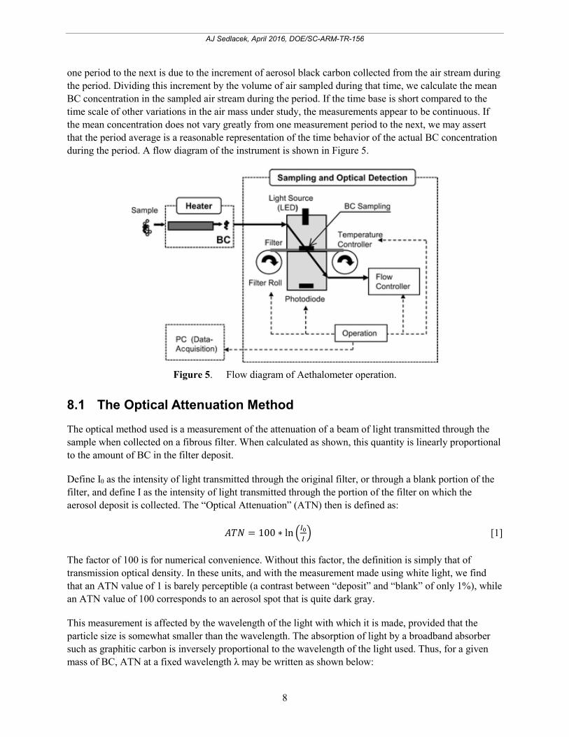
one period to the next is due to the increment of aerosol black carbon collected from the air stream during the period. Dividing this increment by the volume of air sampled during that time, we calculate the mean BC concentration in the sampled air stream during the period. If the time base is short compared to the time scale of other variations in the air mass under study, the measurements appear to be continuous. If the mean concentration does not vary greatly from one measurement period to the next, we may assert that the period average is a reasonable representation of the time behavior of the actual BC concentration during the period. A flow diagram of the instrument is shown in Figure 5.

Figure 5. Flow diagram of Aethalometer operation.

8.1 The Optical Attenuation Method

The optical method used is a measurement of the attenuation of a beam of light transmitted through the sample when collected on a fibrous filter. When calculated as shown, this quantity is linearly proportional to the amount of BC in the filter deposit.

Define I0 as the intensity of light transmitted through the original filter, or through a blank portion of the filter, and define I as the intensity of light transmitted through the portion of the filter on which the aerosol deposit is collected. The “Optical Attenuation” (ATN) then is defined as:

ܣ = 100 כ ln ቀூబூ ቁ [1]

The factor of 100 is for numerical convenience. Without this factor, the definition is simply that of transmission optical density. In these units, and with the measurement made using white light, we find that an ATN value of 1 is barely perceptible (a contrast between “deposit” and “blank” of only 1%), while an ATN value of 100 corresponds to an aerosol spot that is quite dark gray.

This measurement is affected by the wavelength of the light with which it is made, provided that the particle size is somewhat smaller than the wavelength. The absorption of light by a broadband absorber such as graphitic carbon is inversely proportional to the wavelength of the light used. Thus, for a given PDVV�RI�%&��$71�DW�D�IL[HG�ZDYHOHQJWK�Ȝ�PD\�EH�ZULWWHQ�DV�VKRZQ�EHORZ�


9

(ɉ)ܣ = ߪ ቀଵቁ כ [2] [ܥܤ]

ZKHUH�>%&@�LV�WKH�PDVV�RI�EODFN�FDUERQ�DQG�ı��Ȝ��LV�WKH�RSWLFDO�DEVRUSWLRQ�FURVV�VHFWLRQ��“sigma”) that is wavelength-dependent, which is referred to as the “Specific Attenuation.”

Aethalometers operate at one or more fixed wavelengths so the optical intensity functions are products of terms that may or may not be wavelength-dependent. The intensity of light detected after passing through a blank (i.e., clean) portion of the filter is:

(ɉ)ܫ = (ɉ)ܮܫ כ (ɉ)ܨ כ (ɉ)ܥ כ [3] (ɉ)ܦwhere: ,/�Ȝ� is the emission intensity of the light source )�Ȝ� is the spectral transmission function through the filter 2&�Ȝ� is the spectral transmission function through all the other optical components '�Ȝ� is the spectral response function of the detector.

If we now measure the optical transmission through an aerosol deposit on this filter using the same light source and detector, the net intensity will be:

ܫ = (ɉ)ܫ כ exp {െA(ɉ)} [4]

where the absorbance is

(ɉ)ܣ = ቀଵቁ כ [5] [ܥܤ]

and [BC] is the amount which has an optical absorption inversely proportional to the wavelength.

The logarithmic ratio of I to I0, giving the ATN, is therefore proportional to the mass of absorbing BC, ZLWK�WKH�ZDYHOHQJWK�GHSHQGHQFH�RI�RSWLFDO�FRPSRQHQWV�DQG�GHWHFWRU�EHLQJ�ZHLJKWHG�E\�WKH��Ȝ�IXQFWLRQ. The coefficient of this proportionality is defined as the “specific attenuation,” usually referred to as “sigma.”

Note that the derivations described above assume that the actual optical absorption is linearly proportional to the mass of absorbing material. This assumption is valid under the following conditions that are found to apply in practice:

x The particle VL]HV�DUH�FRQVLGHUDEO\�VPDOOHU�WKDQ�WKH�ZDYHOHQJWK�VL]H�SDUDPHWHU�� ʌ Ȝ�

x The amount of absorbing material in the sample is not so great as to lead to saturation.

x The effect of the embedment of the aerosol particles in a deep matrix of optically scattering fibers is to eliminate any reduction of the optical transmission through the filter by optical scattering by the particles, and to render the measurement sensitive to absorption only.

These conditions are met when we sample ambient aerosols on quartz fiber filters and limit the measured optical attenuation to values of approximately 150 or less. Under these conditions, the measured attenuation is found to be linearly proportional to the mass of “black carbon” determined by chemical


10

procedures as defined above. The coefficient of proportionality is the “specific attenuation,” ே . From Eq. [4,] this now is expressed as follows:

ߪ ቀଵቁ = ே = 100 כ ቀଵቁ [6]

The Aethalometer model AE-16 uses a solid-state source operating in the near-infrared at a wavelength of 880 nm. Other models of Aethalometer use other wavelengths, as will be discussed below, and the algorithm must always use the appropriate value of “specific attenuation” that is correct for the wavelength of measurement. This quantity is frequently simply referred to as “sigma,” the specific attenuation with units measured in square meters per gram. Note that it is essential to remember that “sigma” is not a “physical constant” but is wavelength-dependent, and its value must be ultimately related to a chemical or other standard measurement.

8.2 The Aethalometer Algorithm

The algorithm that the Aethalometer system uses to calculate the aerosol BC content of a sampled air stream is based on the following information:

x Measurements of the Reference Beam and Sensing Beam detector outputs with the lamps OFF to determine their zero offsets.

x Measurements of the Reference Beam and Sensing Beam detector outputs with the lamps ON to determine the transmitted light intensities.

x Measurement of the air flow through the system.

x Knowledge of the active collecting area of the spot on the filter, and of the specific attenuation of the particular combination of light source, detector, optical components, and the filter medium in use. (see Chapter 2.0).

Note that the algorithm uses only ratios, with the “zero” levels subtracted, so the results do not depend on any scaling, offset, or proportionality constant of the photodetectors’ response. The only requirement is that the response be linear with respect to the incident light intensity. Understanding what the detector signals exactly represent is not needed to calculate BC concentrations from the measurements.

For the following discussion, we use the following notation:

SB Sensing Beam detector output with lamps on (“Beam Sig” in notation cited in Section 7.8)

SZ Sensing Beam detector Zero offset output with lamps off. (“Zero Sig” in notation cited in Section 7.8)

RB Reference Beam detector output with lamps on (“Ref Beam” in notation cited in Section 7.8)

RZ Reference beam detector Zero output with lamps off (“Ref Zero” in notation cited in Section7.8)

A Aerosol collecting spot area of filter (cm²)

F Flow rate of air through filter, L/min

T Sampling time base period, minutes


11

ATN Optical attenuation due to aerosol deposit on filter (“Opti Atten” in notation cited in Section 7.8)

B Surface loading of BC on filter (g/cm²)

SG Specific attenuation cross section for the aerosol black carbon deposit on this filter, using the optical components of this instrument (m²/g)

BC Concentration of BC in the sampled air stream (ng/cm²).

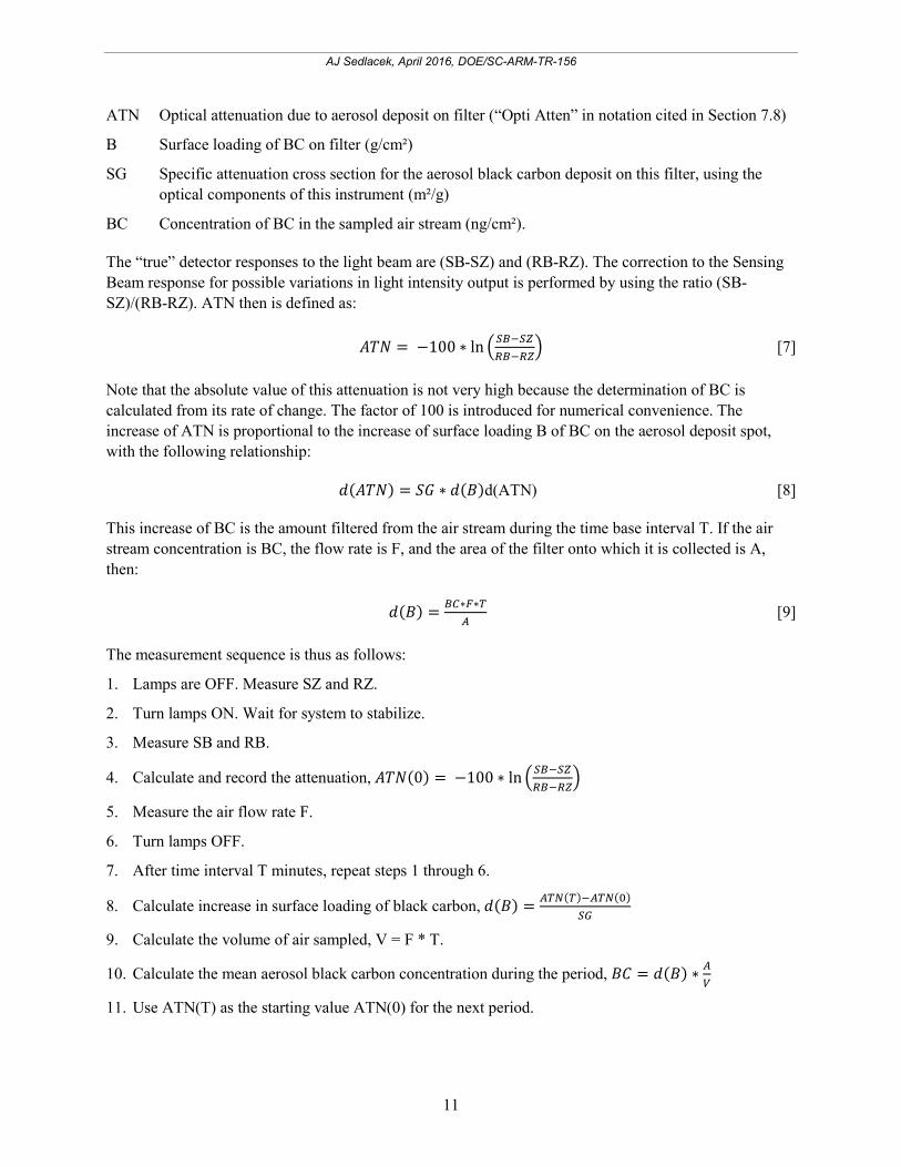
The “true” detector responses to the light beam are (SB-SZ) and (RB-RZ). The correction to the Sensing Beam response for possible variations in light intensity output is performed by using the ratio (SB-SZ)/(RB-RZ). ATN then is defined as:

ܣ = െ100 כ ln ቀௌௌோோቁ [7]

Note that the absolute value of this attenuation is not very high because the determination of BC is calculated from its rate of change. The factor of 100 is introduced for numerical convenience. The increase of ATN is proportional to the increase of surface loading B of BC on the aerosol deposit spot, with the following relationship:

(ܣ) = ܩ כ d(ATN) [8](ܤ)

This increase of BC is the amount filtered from the air stream during the time base interval T. If the air stream concentration is BC, the flow rate is F, and the area of the filter onto which it is collected is A, then:

(ܤ) = כிכ [9]

The measurement sequence is thus as follows:

1. Lamps are OFF. Measure SZ and RZ.

2. Turn lamps ON. Wait for system to stabilize.

3. Measure SB and RB.

4. Calculate and record the attenuation, (0)ܣ = െ100 כ ln ቀௌௌோோቁ

5. Measure the air flow rate F.

6. Turn lamps OFF.

7. After time interval T minutes, repeat steps 1 through 6.

8. Calculate increase in surface loading of black carbon, (ܤ) = ே()ே()ௌ

9. Calculate the volume of air sampled, V = F * T.

10. Calculate the mean aerosol black carbon concentration during the period, ܥܤ = (ܤ) כ

11. Use ATN(T) as the starting value ATN(0) for the next period.


12

9.0 Setup and Operation of Instrument

9.1 Assumption: The Hardware Is Already Setup in the Mobile Aerosol Observing System Container

For normal use, switch the Aethalometer “On” and “Off” using only the switch on the front panel.

Remove the “Filter Protection Strip” that is installed during shipment/transport for protection. Switch the instrument “On,” press the “Tape Advance” switch in the upwards direction, pull the filter protection strip out to the right, and switch the instrument “Off.”

9.2 Quick Setup Summary Guide 1. To Start. Plug in to power source and switch on using the front panel switch. Connect external pump

if required. Instrument starts automatically without any operator attention. Data collection will begin after about 5 minutes. Note: instrument takes about 30 minutes to warm up and stabilize.

2. To Stop Quickly. Simply switch off using the front panel switch. Data file on disk will be current up to this time.

3. To Exit Cleanly with Data Summary. Press STOP key, observe screen. Press STOP key again. Enter “Security Code” (factory default = 111). Summary file will be written to disk.

4. Data Diskette Removal. Data diskette may be removed and exchanged at any time with a fresh disk: does not interfere with data collection.

5. Setting Flow Rate in Software. Flow may be set to read out in “Standard” units (sea level) or “Volumetric” units (adjusted for altitude and temperature).

6. Changing Settings

x Switch on, observe opening countdown screen. Press any key to get top item in Main Menu, “Operate.” Press down-arrow for next menu item “Change Settings.” Press “Enter”.

x Scroll through settings list with down-arrow. Press “Enter” to access an item.

x First item is “Date & Time.”

x Next item is “Timebase,” which usually is set to 1 to 5 minutes, depending on need.

x Next item is “Flow Rate,” which usually set to 2 to 4 liters per minute (LPM).

x To change an item, use arrow keys, make a selection, press “Enter” to confirm, press “Esc” to escape from the systems-settings menu. Confirm change.

7. Data Tradeoffs

x Shorter time base will provide better response to rapid changes in concentration, but noisier data. Note: data can always be smoothed afterwards to reduce noise.

x Suggest running initially at 5-minute time base. Note: electronic digitization noise is drastically UHGXFHG�DW�WLPHEDVHV��PLQXWHV�


13

x Higher flow rate will provide less noise, but shorter lifetime of the tape spot. When the spot saturates, the tape automatically advances. Data will be interrupted for few minutes.

x Increase flowrate to reduce noise on data if tape advance intervals are acceptable.

9.3 Filter Tape Installation

The instrument is shipped with a fresh roll of quartz fiber sampling tape installed on the left “supply” spool. This roll provides 1500 sampling spot locations. Each spot lasts from a few hours in cities to as long as several months at remote locations, and so changing the tape roll is required only occasionally. The display screen shows an estimate of the percentage of the tape roll that remains. When the estimate on the screen falls below 10%, a yellow “Check” lamp on the display panel will light up.

Note that the “Tape Remaining” percentage is a software-based estimate, not an actual measurement of the tape spool. Under some conditions, the estimate can become inaccurate and reach zero even though more filter tape is on the supply spool. Even if the yellow “Check” lamp is lit, and a warning message is displayed on the screen, the instrument will continue to provide valid data until the filter tape actually runs out.

x When the tape is eventually all used, it is necessary to install a fresh roll using the procedures described in Sections 9.4 and 9.5. The menu option “Install New Tape” offers an abbreviated set of sequential instructions with prompts to guide the user through the necessary steps. This software procedure also resets the tape supply percentage counter to 100%.

x For this reason, the “Install New Tape” software procedure must be used when installing a fresh roll of tape. If you are familiar with the procedure, you may bypass the screen instructions, but you must use the procedure in order to reset the counter.

The “Install New Tape” procedure is ‘protected’ and requires the Security Code as a password.

The first list of instructions below describes the actual procedures. The second list shows the prompts displayed on the screen by the “Install New Tape” procedure.

9.4 Install New Tape – Operator Actions – Rack-Mount Models 1. Stop measurements, and turn off the pump (if external). Do not switch off the instrument power.

2. Select “Install New Tape” from the Main Menu.

3. Remove the two thumb screws securing the analyzer chamber center cover plate.

4. Remove the two thumb screws securing the clear plastic front spool flanges.

5. Pull out the gray plastic guide rod (with banana jack) on the left side of the analyzer chamber.

6. Use scissors to cut the tape on the left side (i.e., the supply side). Leave a few centimeters.

7. Remove the unused portion of the previous roll of tape from the supply side spindle. Open the box of new tape, and remove the new roll.

8. Put the new roll of tape on the supply side spindle.


14

9. Using adhesive tape, fasten the starting end of the new filter tape to the end of the old tape on the left side of the analyzer chamber.

10. Press and hold the “Tape Advance” button with your left hand. The inlet assembly will lift about 2 mm, which just enough to release the clamping force on the tape.

11. With your right hand, pull the old tape to the right, with the new tape fastened to it. Pull about 20 cm. of new tape through. Cut off the old tape.

12. Remove the filled spool of used tape from the right hand (i.e., the take-up) side. Unroll it to retrieve the brass spring clip and the cardboard center. Discard the used filter tape, but retain the clip and the cardboard center of the roll.

13. Do not dislodge the O-ring which is behind the cardboard center.

14. Put the empty cardboard center onto the take-up hub.

15. Unwind about 10 cm of the new tape, and thread it under the swinging roller arm that controls the tension. Clamp the end of the tape under the spring clip onto the cardboard center. Turn the cardboard center counter-clockwise to roll the slack tape onto itself.

16. Replace the clear flange on the supply spool side. Tighten the thumb screw firmly but not excessively. Pull on the unrolling portion on the left to check that the supply roll can turn against a little friction. Plug the guide rod back in to its banana jack.

17. Replace the clear flange on the take-up spool side. Tightening the thumb screw clamps the cardboard hub against the O-ring behind it, which provides friction to advance the tape.

18. Press the “Tape Tension” switch, and roll up any slack tape on the right-hand side.

19. Replace the analyzer chamber cover plate and its two thumb screws.

9.5 Install New Tape – Software Procedure Prompts

The first screen asks “List Instructions?” If NO is selected, the instrument assumes that the operator is familiar with the tape installation procedure, and will not require guidance. The software skips the detailed instructions; resets the tape counter to 100%, and returns to the Main Menu.

If YES is selected, the display screen guides the user through all the operations required for changing the tape. After each phrase, the user must press any key to proceed to the next step:

1. Remove spool screws

2. Remove cover screws

3. Pull out guide rod

4. Cut old tape

5. Remove supply roll

6. Remove take-up roll

7. Install new roll

8. Lift up chamber 2 mm


15

9. Push tape through

10. Lift up chamber 2 mm

11. Pull 10 cm tape

12. Install take-up hub

13. Clip tape to hub

14. Push in guide rod

15. Replace cover

16. Replace spools

17. Tighten spool screws.

The screen then asks, “Is the tape properly replaced?” Selecting YES will reset the tape counter to 100% and finish the process.

10.0 Software

Specific for the U.S. Department of Energy (DOE) Atmospheric Radiation Measurement (ARM) Climate Research Facility, the serial output is collected by a LabVIEW shell program that saves data to an hourly file every 5 minutes (when a new set of measurements is available in the queue). The datastream headers are listed in Section 7.8.

The following discussion is specific to the internal software of the Aethalometer and is provided for completeness. Each of these models of Aethalometer is controlled by an embedded 486-class, single-board computer with 4-MB dynamic RAM and 2-MB solid-state disk for program storage. Its digital input/output is used to acquire signals from the electronics and to control internal functions. One of its serial ports is used to communicate with the display panel, which has a four-line, 20-character backlit display screen; a 25-button keypad, and five programmable LED lamps to indicate instrument status. The other serial port provides digital data output to a connector on the rear panel.

The Aethalometer has a 3.5-inch floppy disk drive for data recording. Optionally, a Personal Computer Memory Card International Association (PCMCIA) solid-state memory card drive may be substituted for the floppy disk drive. A digital-analog converter is connected to terminals on the rear panel and provides an output voltage proportional to the measured BC concentration, or a programmable alarm function. The computer with its permanently stored program will start operation automatically upon power-up without any operator intervention necessary.

The software is written as an executable program file, accompanied by parameter files. These are stored in the computer’s permanent memory and do not need to be accessed for routine operation.

The program is operated almost entirely by selection from menus. Choices are presented sequentially in a scrolling list, representing the various appropriate actions at any stage. The choices are selected by moving the up- and down-arrow keys. The first choice is the “preferred” selection (i.e., the most likely response, the current state of a selection that is logical to preserve, etc.). To maintain this choice, simply


16

press the “Enter” key. The instrument can be run through a complete operation to measure aerosol BC by always selecting the presented items, using no key other than “Enter.”

At some points in the program, there may be a need for numerical input from the operator. A flashing underscore cursor ( _ ) is shown on the screen at the input position. As numbers are typed, they are added to the input line. When the line is complete, press “Enter.” If a typing error occurs, press the backspace key “BKSP” to erase the error.

The menu selection and parameter input program units incorporate a timer. The purpose of this timer is to handle the possibility that the operator is called away or distracted by other demands while in the middle of interacting with the Aethalometer. If a menu of items is displayed with an instruction to select just one, or if a numerical parameter is required, the computer will alert the user with a beeping sound after 10 to 30 seconds of no keyboard activity. This is a reminder that operator input is required. This beeping will continue for 10 minutes, at which time the system will execute an automatic restart. This mode is designed to take care of situations where the instrument was ready to run, parameters were being set up, and the operator is distracted (e.g., by a telephone call) in the middle of selecting choices.

If the system halts because of “SERIOUS” problems, the timer is disabled so the screen displays the fault condition message indefinitely until the operator presses a key to acknowledge the problem.

10.1 Use of the Keypad x To scroll through the menus, use the UP- and DOWN-arrow keys. Some menus (e.g., Time & Date)

also use the LEFT- and RIGHT-arrow keys.

x To enter a selected menu, or to confirm a setting, press the “Enter” key.

x To escape from a selected menu, press the “ESC” key.

x When entering parameter values in Change Settings sub-menus, allowable selections are shown by scrolling with the UP- and DOWN-arrow keys; entries are confirmed by pressing the “Enter” key, or canceled by the “ESC” key.

x When the instrument is running, use the “STOP” key to return to the Main System Menu.

Response Time-Out: In most menus for which user input is required, an automatic time-out feature allows the instrument to recover and resume operation if the operator is called away or fails to respond. After 30 seconds, the alert beeper sounds, and if the user does not respond within 10 minutes, the instrument reboots and runs in automatic operation mode.

10.2 Menu Tree

The following chart shows the complete tree of Aethalometer software commands: they are described in detail in the subsequent sections of this chapter.

1. Operate

1.1 *R�WR�$XWRPDWLF�0RGH"�><(6@�ĺ��

1.2 [NO]


17

1.2.1 Flow stabilization period (30 sec.)

1.2.2 Titles

1.2.2.1 Retain old titles

��5HDG�QHZ�WLWOHVĺ�LQVHUW�GLVNHWWH�ZLWK�QHZ�WLWOHV

1.2.3 Verify timebase: OK / Change

1.2.4 Display flowrate for verification

1.2.5 Check diskette data capacity

1.2.5.1 Continue ( = use existing disk)

1.2.5.2 New disk entered

1.2.5.3 Delete oldest files (use if insufficient space on disk)

1.3 Advance Tape, start measurement sequence

2. Change Settings

2.1 Time & Date

2.1.1. Use Left/Right arrow keys to move blinking cursor

2.1.2. Use Up-/Down-arrow keys to change selected value

2.2 Set Flowrate

2.3 Timebase

2.3.1. Use Up-/Down-arrow keys to change value

2.4 Tape Saver

2.4.1 Off

2.4.2 X3

2.4.3 X10

2.5 Analog Output Port

2.5.1 Signal Output

2.5.1.1 Enter scaling factor

2.5.2. Alarm

2.5.2.1 Alarm On/Off

2.5.2.2 Alarm setpoint

2.6 Warm Up Wait

2.7 Communications Parameters

2.7.1 Communication mode

2.7.1.1 Dataline


18

2.7.1.2 Gesytec

2.7.1.3 GPS

2.7.1.4 Off

2.7.2 Baud rate

2.7.3 Data bits

2.7.4 Stop bits

2.7.5 Parity

2.8 Overwrite Old Data

2.9 Filter Change Period (note! Set to ZERO for automatic tape advance)

2.10 Security Code

2.11 Date Format

2.11.1 US (MMDDYY)

2.11.2 Euro (DDMMYY)

2.12 BC display unit

2.12.1 Nanograms per m³

2.12.2 Micrograms per m³

2.13 Data Format

2.13.1 Expanded

2.13.2 Compressed

2.14 UV Channel On/Off (for 2-wavelength instruments)

2.15 Hardware Configuration

2.15.1 Instrument type

2.15.1.1 AE1x – “Standard”

2.15.1.2 AE2x – “UV + LED”

2.15.1.3 AE3x – “7 x LED”

2.15.2 Portable/Stationary

2.15.2.1 “Stationary” – i.e., rack-mount chassis

2.15.2.2 “Portable” – i.e., AE4x series

2.15.3 Spot Size

2.15.3.1 Extended Range (i.e., “larger” 1.67 cm² spot)

2.15.3.2 Standard Range (i.e., “smaller” 0.5 cm² spot)

2.15.4 Serial Number


19

2.15.5 PCMCIA (memory card) enablement

2.16 Gesytec ID

2.17 Sigma for lamps

2.18 Spots per Advance

2.19 Maximum Attenuation

2.20 Return

3. Signals + Flow

3.1 Use Up-/Down-arrow keys to control lamps

3.2 Use Left-/Right-arrow keys to control flow bypass valve

4. Self Test

4.1 Lamp test (1, 2 or 7 lamps)

4.2 Pump and Bypass Valve test

4.3 Analog Output Port test: allows for testing external analog dataloggers

4.4 COM Port test: allows for testing external digital dataloggers

4.5 Display Screen test

4.6 Tape Advance test

5. Calibrate Flowmeter

5.1 Air volume units

5.1.1 Standard

5.1.2 Volumetric

5.1.2.1 Barometric Pressure (millibars)

5.1.2.2 Ambient Air Temperature (ºC)

��)ORZPHWHU�&DOLEUDWLRQ"�>12@�ĺ�UHWXUQ

5.3 [YES]

5.3.1 Measure zero offset (wait for pump to stop – 2 minutes)

5.3.2 Measure active flow (use external flow calibrator, enter factor)

6. Software Upload

7. Optical Test

7.1 Insert floppy disk

7.2 Remove filter tape

7.3 Insert Optical Test Strip

8. Install New Tape


20

8.1 List Instructions?

��><(6@�ĺ�OLVW�RI�WDSH�LQVWDOODWLRQ�LQVWUXFWLRQV

10.3 Main System Menu upon Power-Up

The opening screen displays an opening “Aethalometer” logo; the software version number; a countdown from 60 seconds for the automatic start; and the prompt to “Press Any Key for Main Menu.”

If any key was pressed during the 60-second Countdown, the Main System Menu starts at the top of the list (i.e., Operate). The Main Menu offers the following selections:

1. Operate

2. Change Settings

3. Signals + Flow

4. Self Test

5. Calibrate Flowmeter

6. Software Upgrade

7. Optical Test

8. Install New Tape

Note: For further detail on each of these menu items, see the Software section of the Aethalometer Manual: http://www.mageesci.com/images/stories/docs/Aethalometer_book_2005.07.03.pdf.

10.4 Data File Format

The full data set is written to the disk file “BCxxxxxx.CSV.” Two formats are offered, both of which are written in a single line as “Comma-Separated Variable” (CSV) data to allow immediate import into a spreadsheet.

10.4.1 Format Types

The two file formats, Expanded Data Format and Compressed Data Format, are described below.

10.4.1.1 Expanded Data Format

The Expanded Datat Format in the following information: date, time, BC concentration (ng/m3), sensing zero signal, sensing beam signal, reference zero signal, reference beam signal, air flow (LPM), bypass fraction, optical attenuation. A typical line in the data file might look like:

“01-may-99”, “09:40”, 866, .0213, 2.1956, .0241, 3.1455, 4.2, 1.00, 1.974

Note that the recorded time corresponds to the starting time of the measurement cycle.



21

Only the date, time, and BC concentration are used in normal circumstances: that is, the first three columns of data as shown in bold in the above example. The other columns of data only verify correct operation of the instrument. For this reason, data may also be written in a compressed mode, which preserves the diagnostics but in a more compact form.

10.4.1.2 Compressed Data Format

The Compressed Data Format includes date, time, BC concentration (ng/m3), and “codeword.” In compressed’ format, the same line in the data file might look like:

“01-may-99”, “09:40”, 866, “fpXeoenmRBqlaYdh”

The codeword is a 16-element string of upper- and lower-case alpha characters whose American Standard Code for Information Exchange (ASCII) codes represent the numerical data exactly.

No diagnostic data are lost in the compression process: they are simply compacted into a coded format. The data line may be decoded using the utility program COMDECOM available from Magee Scientific.

This decoding program produces a new file in the full “Expanded” data format. However, in many situations, the internal diagnostic data represented by the codeword are unnecessary—all that is needed are the date, time, and BC concentration. In those cases, the fourth column of CSV data, namely the codeword, may be simply discarded for the purposes of data analysis and display.

Note also that, because the “compressed” data format contains fewer characters per data line, the data capacity of a floppy diskette is greatly increased if the data are written in compressed mode. This is particularly true for multiple-wavelength instruments.

10.4.2 Data Continuation

The Tape Advance process takes a few minutes before the instrument is reinitialized and valid data are again being produced. If the Timebase value is 10 minutes or longer, there is always at least one valid “innerloop” measurement so the data file record is continuous. However, if the Timebase value is shorter than 10 minutes, there will be some time base starting times for which no valid data exists. If these start times were simply ignored, the continuous data record would contain “missing” values that would require manual editing to identify if the BC data were to be aligned with other measurements.

To avoid these ‘missing’ entries, the software automatically writes blank data lines to disk at values of the start time that correspond to the Timebase sequence. These blank “filler” lines contain valid values of date and time, but the remainder of the data entries consist of ASCII nulls enclosed in double quotes and separated by commas. This allows the entire data record to be imported into a spreadsheet in CSV format, and to yield blank (not numeric-zero) entries.

See the Aethalometer Manual for information regarding the data file format for dual-wavelength and seven-wavelength instruments. The manual can be accessed on the Internet at http://www.mageesci.com/images/stories/docs/Aethalometer_book_2005.07.03.pdf.



22

10.4.3 “Message” File Contents

The message file name is constructed from the characters “MF” followed by six digits compounded from the date on which the file was opened, followed by the extension “.TXT.” The file entries are all ASCII text strings that may be directly viewed by any word processor.

Entries posted at distinctly different times contain the date and time as the first lines. The entries generally provide the following information:

x Date and time of measurements starting

x Optical signals at start

x Date and time of measurement ending

x Optical signals at end

x A summary of the run of a filter spot, including:

– Total aerosol BC collected on filter

– Total filter spot running time

– Total sampled air volume

– Mean BC concentration during filter running period

– Standard deviation of BC measurements

x Comments on the performance of the instrument, and the stability of the lamp

x An estimate of the remaining data disk capacity.

If any instrument problems are encountered, additional messages are posted. Serious problems cause measurements to halt until operator attention is provided, with a warning message displayed on the screen.

These occurrences also are posted to the message file to provide a record in case the entire system goes down. Serious problems include loss of air flow because of pump failure or blockage of the plumbing, failure of the lamp, or other problems with the lamp control, etc. In addition, a message is posted each time the tape advances one spot. Other messages that are self-explanatory may occasionally be generated by particular conditions.

10.5 Screen Display: Normal Operation

First line: Left: system time Right: system date

Second line: Left: (Tape:) estimated amount of tape roll remaining Right: (Saver:) “Tape Saver” feature activation status

Third line: Left: (Disk:) free space on disk, expressed as hours, days, or weeks. Right: (Flow:) air flow in LPM: “vLPM” indicates use of volumetric units.


23

Fourth line: /DVW�YDOXH�RI�%&�FRQFHQWUDWLRQ�LQ�ȝJ�P3 or ng/m3.

The front panel has five programmable Status Indicator Lamps to indicate the instrument status:

x RUN (green)

– Steady: Normal operation, measurement data is valid.

– Flashing: Normal operation, but there is no valid data because the instrument is performing a tape advance or (re-) initializing.

x PAUSE (yellow): Indicates that the instrument is ready for measurements, but was stopped by the operator pressing the “STOP” key. Also displayed in manual mode in the operate procedure until all operator interactions are completed.

x CHECK (yellow): Flashing indicates something must be checked: data disk almost full, tape almost all used, or air flow rate has changed more than 10%.

x ERROR (red): Flashing. A serious error has occurred, and the instrument has stopped.

x STOP (red): Instrument is not ready to run. It was stopped either by a serious error or when operator is in a menu/setup mode.

11.0 Calibration

The Aethalometer requires no calibration other than periodic checks of the air flowmeter response.

If there is reason to believe that the flowmeter reading is inaccurate, a flowmeter recalibration should be performed.

This program first allows the user to switch between “Standard” and “Volumetric” flow units. (If “Volumetric” flow units are selected, it is necessary to input the barometric pressure and ambient air temperature). This function is not password protected. The program next allows the user to recalibrate the flowmeter: this function is protected.

x Flow Volume Units. The program allows the flow to be expressed in terms of either Standard Units or Volumetric Units.

Standard Units report the air flow rate as standard liters per minute (SLPM) (i.e., volume occupied by a given mass of air at a temperature of 20ºC and a pressure of 1013 mbar). This mass flow rate is the signal that is provided by the mass flowmeter in the instrument. The Aethalometer data is reported as ng/m³ or g/m³, where the “m³” is understood to be a standard cubic meter.

Volumetric Units convert the mass of air to a volume calculated at certain specified ambient conditions of temperature and pressure. These conditions must be entered by the user; they are not measured by the instrument. The mass flow rate signal provided by the mass flowmeter is scaled by proportionality factors for temperature (input in degrees Celsius) and pressure (input in millibars). When volumetric units are selected for the flow, the flow rate display on the screen is shown as v/30��DQG�WKH�%&�FDOFXODWLRQ�LV�SUHVHQWHG�DV�QJ�YPñ�RU�ȝJ�YPñ��


24

The volumetric calculation requires user input of ambient temperature and pressure. These factors may be entered without going through the flowmeter recalibration procedure. This allows different mean ambient temperatures to be entered or different pressures if the instrument is moved to a location of different elevation, without disturbing the fundamental calibration of the mass low meter response.

Note: The ‘Portable’ series of instruments use a different type of flow sensor with an output that is not a representation of air mass flow, but intrinsically depends on ambient pressure. For precise operation at reduced ambient pressure, the ‘Portable’ instrument should be recalibrated under ambient conditions.

x Flowmeter Recalibration. This is a ‘protected’ function and requires the Security Code as a password.

This procedure calibrates the flowmeter response by measuring the flowmeter zero voltage and determining the flow scale factor. These two factors are used during measurements to calculate the actual air flow through the flowmeter.

Notes:

– You will need a standard external flowmeter or calibrator capable of reading air flow rates in the range of 2 to 10 SLPM, with a low resistance to flow. Connect this calibrator firmly to the Sample Inlet Port with no possibility of an air leak.

– Only perform this recalibration if you have serious reason to believe that the flowmeter response is incorrect.

– Allow the instrument to warm up for at least 30 minutes with power and air flow ON before performing the recalibration.

– See above for discussion of standard vs. volumetric units.

The internal pump is controlled by the computer and electronics, and this allows the program to set “zero” and “span” flows. All that is required of the operator is to connect a standard external flow calibrator, and observe its reading. The routine first automatically reduces the pump speed slowly to zero, while measuring the signal from the internal flowmeter. When a steady low value is reached as determined by no more change in voltage output, the value of the reading is used as the flowmeter zero voltage. The pump is then restarted and run up to its previous speed. When the flowmeter signal is steady, the screen displays the flowrate in liters per minute derived from the new zero and the previous scale factor. The user must then compare the displayed value of flow with the actual value as measured by the external standard. Pressing the keypad UP- and DOWN-arrow keys will change the flow scale factor. Press these keys until the displayed value agrees with the measurement from the external calibrator. Press “Enter” when the displayed value is correct. Upon return to the main system menu, the user is asked to confirm writing the newly measured response factors to the setup file. The previous flow calibration values are not replaced until this confirmation is made. In case of any doubt, repeat the procedure.


25

12.0 Maintenance

12.1 Disassembly and Cleaning

The optical sampling and analysis cylinder should be removed and cleaned once every year or two, or at any time if there has been the possibility that foreign material such as insects, macroscopic dust, fluff, etc., has been drawn into the instrument. This schedule may be accelerated in situations of high aerosol loading. A good guideline would be to perform the cleaning every second time a roll of tape is installed. The disassembly and cleaning procedure takes less than 30 minutes, requires no special tools or special skills, and the instrument may be reassembled without any concerns about critical alignment or re-positioning of any components. The disassembly and cleaning procedure is described below:

1. Remove the top and bottom instrument cover plates (four screws each). Note the electrical grounding wires on tab connectors. The lower cover plate has a layer of black rubber thermal insulation.

2. Remove the light shield covering the analysis chamber (two thumb screws).

3. Turn the instrument over so its underside is facing up. Remove the hose clamps that secure the sampling hose to the tube on the aerosol inlet fitting. Use a small screwdriver to slide apart the two sets of gripping teeth. Disconnect the angled flexible black tubing that goes from the inlet port up and through the chassis plate to the analysis chamber.

4. Push the inlet tube through the slot in the chassis plate to the upper side, so that it is loose.

5. Turn the instrument back over so the underside is facing down. From the front, unscrew the knurled cap on top of the analysis chamber. Note the electrical ribbon cable passing through.

6. Lift up on the knurled cap, gently push approximately 1 cm of ribbon cable through the grommet in the cap.

7. Note the 10-pin flat cable connector inside on the right. Pull up on the cable GENTLY to pull the connector plug out of its socket. This is the power to the optical source assembly. In some cases, the optical source assembly may lift up on the end of the cable and come out of the top of the cylinder. If so, it is not necessary to disconnect the plug.

8. Move the knurled cap to one side, with the cable passing through it and the connector (and possibly also the optical source board) dangling.

9. Remove the spacer ring from under the lifting frame. The spacer ring is approximately 4 cm. in diameter but only 3 mm. thick.

10. There is now enough vertical clearance to lift up and pull out the optical analysis cylinder. The inlet tubing will follow behind like a tail.

11. The optical source assembly is in the top on a small gold-plated circuit board, or possibly loose. Clean it lightly with a soft cloth and alcohol. The sample analysis cylinder is underneath, with two quartz glass windows. The upper window is sealed; the lower window has an opening in the center fitted with a metal ring that defines the collection spot size. The sample air stream enters from the side. Clean the windows (inside and outside) with alcohol and a soft cloth or cotton stick. Run solvent through the tubing and blow it out with low-pressure compressed air. If the optical cylinder is extremely dirty (e.g., if sampling concentrated diesel exhaust), wash the optical cylinder in warm soapy water, then rinse and dry thoroughly with warm air.


26

12. Check the bypass filter cartridge (see next section).

13. Make sure everything is clean, and then reassemble in the reverse order. Replace the optical cylinder; next, reinsert the spacer ring; and finally, reinsert the optical source and/or reconnect its cable. Check the orientation of the optical source assembly. If it had been loose, be sure to relocate it on the two small pins. Observe the tab on the cable plug to the sources. It only goes in one way round. All components are rugged, and there are no critical alignments, provided the source assembly is located on its pins.

14. When replacing the knurled cap, feel that the threads are properly engaged to avoid stripping them when tightening. Check that the optical cylinder and spacer ring are tight against the lifting frame.

15. Push the sample inlet tube down through the chassis plate. Turn the instrument over to its underside and reconnect the tube to the fitting on the rear panel. Replace and tighten the hose clamps.

16. Before replacing the cover plates, run the instrument in “Signals + Flow” test mode. Verify that you get good optical signals with the lamps ON and OFF by using the UP- and DOWN-arrow keys.

12.2 Replacement of Bypass Filter Cartridge

The bypass filter cartridge is located at the rear of the upper chassis, above the sample inlet port. Its flow path is between a side connection to the sample inlet and the bypass valve. When the bypass valve is not activated, pump suction is applied to the filter support grid in the analytical cylinder base, and the sample air stream is drawn from the inlet port through the filter tape. When the bypass valve is activated, pump suction is disconnected from the filter, and is instead connected directly to the sample inlet port through the filter cartridge attached to a side fitting on the inlet. The purpose of the filter cartridge is to remove any particles from this air stream that might otherwise contaminate the bypass valve, the air mass flowmeter, and the pump.

The condition of the bypass filter cartridge does not affect the analytical operation of the Aethalometer, provided it is not completely blocked. Even if it becomes visibly dark, it will not compromise the validity of data from the Aethalometer. The flow resistance of the bypass filter cartridge is always much lower than that of the quartz fiber filter tape. Therefore, even if the cartridge becomes substantially loaded with collected particles, it will not affect the air flow. The reason for changing the bypass filter cartridge is simply to prevent it from becoming completely blocked with dust or other aerosol particles.

The bypass valve is activated only under the following conditions:

1. During filter tape advances. This removes suction from the underside of the filter tape while it is being pulled across the support grid. This reduces the drag on the tape and reduces the probability of scraping quartz fibers from the tape.

2. During operation of the “Tape Saver” mode. This applies a time fractionation to the sample air stream during each time base period, to reduce the number of liters of air from which BC is collected. This reduces the rate of BC accumulation and prolongs the lifetime of each filter spot when concentrations are high.

If “Tape Saver” is not used, very little air flow passes through the bypass filter cartridge: only during tape advances. In this case, the filter cartridge will last a long time before it starts to become visibly dark. If “Tape Saver” is used, sample air will flow through the filter cartridge for a substantial fraction of the


27

operating time, and the filter cartridge will collect a larger deposit of particles. If the bypass filter cartridge is visibly dark, replace it during the routine process of cleaning the inlet cylinder.

The bypass filter is a standard cartridge filter with ¼-inch (6-mm) diameter smooth connection stems for press fitting. Its diameter is 1 inch (25 mm) and its overall length is 3¼ inch (83 mm.). It may be replaced with any equivalent bypass filter. Alternatively, contact Magee Scientific for a free replacement.

To replace the bypass filter cartridge, press on the release ring of the fitting to allow the cartridge stem ends to be pulled out. When inserting the new cartridge, be sure to press the stems firmly into the fittings, to seal them in the internal O-rings.

12.3 Flow Audit: Flowrate Error Scaling

The relationship between an increase in optical attenuation (as defined precisely by the ratio of photodetector signals), and a collected quantity of carbon in a specific “elemental” form, is defined by an absorption cross section per unit mass that is an intrinsic property of the carbonaceous material. This relationship is defined by the “sigma” factor used in the Aethalometer algorithm but does not require periodic calibration or verification. However, knowledge of the number of liters of air from which these nanograms of BC were filtered is required to calculate the concentration result. The mass flowmeter used in the instrument returns a voltage signal proportional to the flow rate of air passing through it, and its recalibration in case of erroneous response is described in the “Calibration” section of this handbook. This recalibration should only be performed if it is believed that the actual flowmeter response itself is inaccurate. However, air flow reporting errors may occur as the result of leaks or blockages. The flowmeter may be reporting its signal correctly, but this may differ from the true flow rate of aerosol sample entering the instrument through its rear-panel sampling port. For example, if the hose connecting the inlet port to the sampling chamber were broken or disconnected, air would be drawn from the interior of the instrument chassis through the filter tape spot and through the flowmeter. The flowmeter might correctly report a flowrate of (say) 4 SLPM, but there would actually be no sample flow at all through the rear-panel connector. Therefore, it is a wise precaution to verify the sampling flowrate by means of a flow audit at periodic intervals.

The Flow Audit is performed by simply connecting a standard flow measuring device to the inlet port, and comparing its reading of air flow entering the Aethalometer to the internal flowmeter signal as reported in the ‘Signals + Flow’ menu mode. Under “normal” operating conditions, the internal flowmeter reading may differ by some percent (e.g., up to 0.5 LPM) because of minor internal leaks, especially air flowing tangentially through the edges of the filter tape. Thus, for example, the internally reported flowrate used by the algorithm may be 4.0 LPM, while actually only 3.8 LPM are entering the sample inlet port on the rear panel, with 0.2 LPM of leakage occurring internally and adding to the flow through the flowmeter, but not representing the actual external air sampled. In such a case, the algorithm is dividing the determined number of nanograms of BC by 4.0 instead of 3.8. The reported data would be too low by a simple scaling factor of 3.8 ÷ 4.0 (i.e., 5%). Correct data will be recovered by simply increasing the reported values by a correction factor of 5%. The scaling is directly proportional to the flowrate error factor.

Even if the flowrate scaling factor differs from unity, the sampling and analytical capabilities of the Aethalometer are not impaired. The optics and electronics still perform an accurate measurement of the


28

increment of BC collected. The only error lies in the assignment of this increment to a certain number of liters of air. If this error can be corrected by simple numerical scaling, the correct result will be recovered.

Recommendation: perform an external flow audit at least once per year, and also before and after any critical study period.

13.0 Safety

Beyond those associated with the operation of any instrument/device that requires 120 V of electricity, there are no additional safety considerations associated with the use of the Aethalometer.

14.0 Citable References

Hansen, ADA. 2007. “Operating Manual for the AE31/22/42 Aethalometers.” Magee Scientific, Berkeley, California. Available at http://www.mageesci.com/images/stories/docs/Aethalometer_book_2005.07.03.pdf.


aethalometer instrument handbook - arm climate … aethalometer instrument handbook aj sedlacek,...

Documents