aesop: an interactive computer program for the … technical paper 2221 january 1984 aesop: an...

NASA Technical Paper 2221

January 1984

AESOP: An Interactive Computer Program for the Desiqn c of Linear Quadratic Regdators and Kalman Filters

Bruce Lehtinen’ and Lucille C . Geyser

https://ntrs.nasa.gov/search.jsp?R=19840008775 2018-05-19T07:26:37+00:00Z

TECH LIBRARY KAFB, NM

NASA Technical Paper 2221

1984

National Aeronautics and Space Administration

Scientific and Technical Information Office

1984

AESOP: An Interactive Computer Program for the Design of Linear Quadratic Regulators and Kalrnan Filters

Bruce Lehtinen and Lucille C. Geyser Lewis Research Center Cleveland, Ohio

Contents

Page Summary ................................................................................................................... 1 Introduction ............................................................................................................... 1 Theoretical Background and Problem Formulation .............................................................. 2

Eigenvalues and Eigenvectors ....................................................................................... 4

Residues ................................................................................................................. 5

Open-Loop System Description .................................................................................... 2

Controllability. Observability. and Mode Shapes .............................................................. 4

Steady-State Linear Quadratic Regulator (LQR) Design ..................................................... 5 Steady-State Kalman Filter Design ................................................................................ 7

Stochastic Linear Quadratic Regulator Design .................................................................. 9 Normalization .......................................................................................................... 7

System Response to Noise Inputs .................................................................................. 9 Transfer Functions and Frequency Response Calculations ................................................. 10 Transient Response Calculation .................................................................................. 13

AESOP Program Operation .......................................................................................... 15 Program Structure ................................................................................................... 15 Operating Procedure ................................................................................................ 15 Data Input and Output ............................................................................................. 19

Description of AESOP Functions ................................................................................... 20 Series 100 - Program Control ..................................................................................... 22 Series 200 - Data Input and Revision ............................................................................ 22 Series 300 -Matrix Formation .................................................................................... 24 Series 400 - Open-Loop System Analysis ....................................................................... 24 Series 500 - Frequency Responses and Bode Plots; and Series 700 - Transfer Functions ............ 25 Series 600 - Transient Responses ................................................................................. 26 Series 800 - LQR and Filter Design .............................................................................. 26 Series 900 - User-Supplied Subroutines ......................................................................... 28

Concluding Remarks ................................................................................................... 28 Appendixes

A - Symbols ........................................................................................................... 30

C - Test Cases ........................................................................................................ 64 Test Case I - Third-Order Problem to Demonstrate Full AESOP Program Capabilities ......... 64 Terminal Printout for Test Case I ...................................... ._. .................................... 65 Test Case I1 - Interactive Design of a Nonzero-Set-Point Regulator .................................. 80

D -Terminal Output Options and Main PROCDEF ....................................................... 102 Standard Terminal Output .................................................................................... 102 Extended Terminal Output .................................................................................... 102 PROCDEFAESRUN .......................................................................................... 103

E - Flow Chart ...................................................................................................... 104 F - Prerequisite Table ............................................................................................. 108

References ............................................................................................................... 111

B - Subroutine Descriptions ....................................................................................... 33

iii

Summary AESOP is a computer program for use in designing

feedback controls and state estimators for linear multivariable systems. AESOP is meant to be used in an interactive manner. Each design task that the program performs is assigned a “function” number. The user accesses these functions either (1) by inputting a list of desired function numbers or (2) by inputting a single function number. In the latter case the choice of the function will in general depend on the results obtained by the previously executed function.

The most important of the AESOP functions are those that design linear quadratic regulators and Kalman filters. The user interacts with the program when using these design functions by inputting design weighting parameters and by viewing graphic displays of designed system responses. Supporting functions are provided that obtain system transient and frequency responses, transfer functions, and covariance matrices. The program can also compute open-loop system information such as stability (eigenvalues), eigenvectors, controllability, and observability.

The program is written in ANSI-66 Fortran for use on an IBM 3033 using TSS 370. Descriptions of all subroutines and results of two test cases are included in the appendixes.

Introduction The computer program called AESOP (Algorithms for

Estimator and Optimal regulator design) was written to solve a number of problems associated with the design of controls and state estimators for linear time-invariant systems. The systems considered are modeled in state- variable form by a set of linear differential and algebraic equations with constant coefficients. Two key problems solved by AESOP are the linear quadratic regulator (LQR) design problem and the steady-state Kalman filter design problem. The remainder of AESOP is devoted to calculations in support of these two problems, mainly for analyzing the open-loop system and evaluating the resulting control or estimator designs. Thus the overall program can be subdivided as follows:

(1) Open-loop system analyses (2) Control and filter design (3) System response calculations The AESOP program was developed at Lewis for use

in conducting design studies in propulsion system control (refs. 1 and 2). AESOP was an outgrowth of a previously developed control design program called LSOCE (ref. 3), which had been used in supersonic inlet controls development (refs. 4 and 5) . AESOP differs from LSOCE mainly in that it was designed to be operated in an interactive

manner, whereas LSOCE was strictly a batch type of program. In addition, AESOP contains system response and evaluation features that are not present in LSOCE. These additions tend to enhance AESOP’S use as an interactive design tool.

Other control design computer programs appearing in the literature perform computations similar to those of AESOP. Notable among the original LQR design programs are ASP by Kalman and Englar (ref. 6) and its Fortran version VASP (ref. 7). Subsequent LQR design packages were the OPTSYS program of Bryson and Hall (ref. 8), the ORACLS program of Armstrong (ref. 9), and Honeywell’s DIGIKON (ref. 10). Computer-aided control system design program development has accelerated in recent years. A good summary of this development is contained in reference 11. Here, over 20 control design programs and packages, including AESOP, are discussed in varying degrees of detail. They represent a variety of design methodologies, ranging from classical single-loop approaches to multivariable LQR and multivariable frequency domain approaches, for both continuous and discrete formulations. Most are written in Fortran and have some sort of interactive capability, but except for a few commercially available packages, most are neither completely documented nor generally available. AESOP, at the present time, is the only interactive LQR type of control design program that is in the public domain. (Contact COSMIC, The University of Georgia, Athens, Ga. 30602, concerning the availability of this program.)

The AESOP program is structured around a list of predefined and numbered functions. Each function performs, basically, a single computation associated with control, estimation, or system response determination. For example, one AESOP function computes the eigenvalues of the open-loop system matrix A, another function reads in the A matrix, etc. These functions are described fully in the section Description of AESOP Functions. The use of these functions and the part they play in AESOP can be described in general terms with the aid of figure 1. The figure illustrates what the user of the program does (left side of fig. l), what the program does (right side of fig. 11, and the interaction between the user and the program.

The user begins by defining the problem to be solved (e.g., by defining the matrices that define the state- variable model of the open-loop system). The user then provides this information to AESOP as input data, generally storing it in a data file. Next the program “prompts” the user to enter a list of function numbers that are to be performed, in sequence, by AESOP to solve the user’s problem. Usually this list of numbers is entered at a terminal, but it can also be entered from a prestored data file. The AESOP program then executes the desired functions in proper sequence, storing away all results on an output file (fig. 1) as “off-line output” but

Figure 1. -Overview of AESOP program operation.

also displaying selected portions of the results back at the user’s terminal (fig. 1) as “on-line display.” The user then decides whether to terminate the program or to request that more functions be performed. The program again prompts the user to enter numbers that define the new functions, which can be entered singly or as a number string. Typically, one of the functions a user would enter, at this time, would be one that allows the user to vary some problem parameter. In this way the user can effectively interact with the program in an online manner to achieve the desired design results. At the conclusion of the terminal session the user commands the output data file to be printed and hard copies to be made of any graphic output generated that was not previously displayed on-line.

This concludes the overview of the basic operation of the AESOP program. The next section describes the various design problems that can be solved by using AESOP, indicating what function numbers the user would request in order to perform the computations. Following that section is the section AESOP Program Operation. Here, examples are presented of a typical dialog between the user and the program. Following that is the section Description of AESOP Functions, which describes each of the 78 functions, what input each requires, and what calculations each performs. These latter two sections serve as a guide to which the user can

2

refer as necessary while running the program. Appendixes include information such as a symbo! table, brief subroutine descriptions, and two test cases that are useful both for program checkout and for gaining an understanding of how the program operates.

Theoretical Background and Problem Formulation

The computations performed by the AESOP program can be grouped into five basic categories. These categories are illustrated in figure 2. This section presents the equations that define the various problems to be solved and indicates the solution methods used by AESOP. After reading this and the next section, the reader should be able to use AESOP to solve a number of “standard” problems by using “standard” sequences of function numbers. The reader will then be able to devise other function number sequences that would allow other more specialized problems to be solved.

Open-Loop System Description

Before beginning any control or filter design on a linear dynamic system, it is important to thoroughly analyze the open-loop system under consideration. The linear open-loop system defined for use throughout this

\U Transfer functions and frequency

system analysis response

LQR and Kalman filter design

System transient responses

I

I 1 System response to noise inputs

Figure 2. -Control system design computations performed by AESOP program.

report is given in the following state-variable form and where shown schematically in figure 3. The state equation is

X = A x + B u + D w (1) v NMth-order white-noise measurement vector

where

Z NMth-order measurement vector

H NM-by-N matrix

x Nth-order state vector u NCth-order control vector

In addition to the measurement vector an output vector, which represents unmeasurable outputs, is defined as

w NDth-order white-noise disturbance vector y = C x+DOUT u (3)

and A, B, and D are matrices of appropriate dimensions. where y is an NOth-order output vector. Finally, a set of Fortran symbols for matrices used in the AESOP noise-free measurements called a set-point vector are program coding are used herein whenever possible. A defined. These represent outputs (NC in number) that are measurement equation, defining the system’s measurable to be regulated to desired constant set-point values. This output vector is vector is given as

z = z 1 + v (2a) ysp=CSP x (4)

z l = H x (2b) where ysp is an NCth-order set-point vector.

Disturbance, w

-++I +J-r Set-point ouQut ysp

Control, u e -

State, x

1

I Figure 3. -Block diagram of open-loop system.

3

Eigenvalues and Eigenvectors

Of prime importance in designing a control system is knowledge of the open-loop system structure and stability. This knowledge affects the designer's choice of performance index weighting matrices, sensed variables to use for control or estimation, etc.

Open-loop stability is determined by the eigenvalues of the system A matrix. The system is stable if and only if these eigenvalues Xi (i = 1, 2, . . ., N) all have negative real parts. Consider the unforced version of equation (I),

X=A x ( 5 )

Define a new state vector X, relating to x through the transformation matrix T as

T X = X -

(6)

Substitute for x in equation ( 5 ) to obtain

- i = ~ - 1 A T X (7)

If we let T- 1 A T be equal to a diagonal matrix A, equation (7) can be rewritten as

-

x = A X (8)

The diagonal elements of A are the eigenvalues of A, T is the eigenvector matrix (a matrix whose columns are the eigenvectors of A), and x is defined as the modal state vector. The value of A is computed by using AESOP function 501, and the eigenvectors are obtained by using function 402. To avoid complex arithmetic, a block diagonal form is used for the matrix A such that a complex eigenvalue pair (hi, Xi+ 1) =(a + j P , a - j P ) appears in the 2-by-2 diagonal block of A,

C Y I - P

P I CY """

where the CY'S are along the diagonal. Let the complex eigenvector pair (vi, vi+ 1 = y + j S , y - jS) correspond to the complex eigenvalue pair CY +jB. Then in the columns corresponding to the defined diagonal block of A there appear two real vectors ti and ti+ 1 defined as

t j=y+S

t i+ l=y-S

4

Hence, when A is block diagonal, T is called a modifid eigenvector matrix. AESOP function 402 also calculates the so-called mode shapes. For a real eigenvector the mode-shape vector is the same as the eigenvector. However, for a complex eigenvector pair the corresponding mode-shape vector pair contains, in successive columns, the magnitude of qi and the phase of qi. Each mode-shape vector is normalized by dividing all of the elements by the magnitude of the largest element. The phase of the largest element is set to zero, and the phases of all other components of the vector are adjusted accordingly.

Controllability, Observability, and Mode Shapes

Once the eigenvalues and eigenvectors (mode-shape vectors) are calculated, it is an easy task to determine controllability and observability. For this purpose, system equations (1) and (2a) can be rewritten in terms of the modal state vector as

G = A x + T - l B u

Z = H T X + V

System controllability is determined elements of T- 1 B. The system is

by examining the uncontrollable if

elements in a row of T - 1 B are zero, meaning that it is impossible to excite a component of the modal state vector x with the control vector u. Also, using this modal formulation, one can think of the matrix T - 1 B as being the control effectiveness matrix. That is, the relative magnitudes of the row elements of T- 1 B define the relative influence each control input has on a modal state variable (mode). For a meaningful comparison, however, the control inputs must be normalized (nondimen- sionalized). Normalization can be done by using AESOP function number 404. Normalization (and unnormalization) is discussed in detail later in this section. The control effectiveness matrix is calculated by AESOP function 403.

System observability can be determined similarly by using the modal state form. From equation (10) it can be seen that, if all elements of column k of the H T matrix are zero, modal state k will be unobservable through measurement z. Also, the relative magnitudes of the elements of row k of H T define the relative contribution each mode makes to measurement zk. This information is useful, for example, if one wishes to minimize the number of measurements (sensors) required when designing a control system that is to shift certain system poles (modes, modal states). System observability (the H T matrix) is computed in AESOP by using function number 403.

In AESOP both the controllability matrix (T - 1 B) and the observability matrix (H T) are printed out in mode- shape format. This means that, for T-1 B, when two successive rows k and k+ 1 relate to a complex modal state pair ( i k , &+ 9, the kth elements in the columns of T- 1 B are magnitudes and the (k + 1)th elements are phase angles. Similarly, for the H T matrix, for a complex modal state pair, elements in the kth column of H T are magnitudes and those in the (k + 1)th column are phase angles.

Residues

The availability of matrices H T and T- 1 B makes it very easy to compute the system residues. Consider the system in modal state vector form given by equations (9) and (10). Let B= T- 1 B and H = H T. Thus equations (9) and (10) can be written as

x = A x + B u

For a single-input-single-output linear system a transfer function g (s) can be written in so-called residue form as

N g ( s ) = E 'j

j = ] s-X,

where each of the N constants rj is defined as a residue at the transfer function pole Xj. The residues define the relative magnitude with which the system input affects the system output through each system pole. This single input/output concept generalizes directly to the multiple input/output case. Here the transfer function matrix G (s) for the system of equations (loa) and (lob) can be written as

or in residue form

where now the N elements Rj are residue matrices. Since A is a diagonal matrix, we can rewrite the matrix ( s I - A ) - ~ as

1 N (sI-A)-l=diag( S-Aj --) = ,=] ,E s Z L -5

where

0'

1

0 \ \ \ \

0

Substituting from equation (100 into equation (loe), we obtain an equation that defines the residue matrices, namely,

Thus the j t h residue matrix is simply

For a real eigenvalue X, the elements of the corresponding residue matrix Rj are real, being computed simply as the (outer) product of thejth column of H and thejth row

For a complex eigenvalue pair (X,, X,+]) AESOP makes use of the modified eigenvector matrix form for T, which means that H and B are also used in that form. Thus real arithmetic can be used in computing the real and imaginary parts of the residue matrix. AESOP prints out that matrix in polar form (one matrix of residue magnitudes followed by one matrix of residue phase angles). The residues are computed along with open-loop controllability and observability checks in function 403.

of B.

Steady-State Linear Quadratic Regulator (LQR) Design

One of the primary functions of the AESOP program is to compute solutions to the steady-state linear quadratic regulator problem. Because this problem has been well documented (ref. 12, e.g.), the results are only briefly summarized herein. The system to be controlled is described by

where the state x is assumed to be measurable and no plant disturbances are present.

A control that minimizes the quadratic performance index

5

J = l , (XTQCX+~XTNNU+UT(PCINV)-~ u)dt (12)

is given by

OD

U= -KC X (13)

For the optimal solution to exist, weighting matrices QC, NN, and PCINV must be as follows:

(1) PCINV is positive-definite (2) QC can be written as QC=M Q MT where the

pair (M,A) is observable and Q is symmetric and positive-definite

(3) QC - NN-PCINV-NNT is nonnegative-definite. Feedback gain matrix KC is found by solving the following matrix Riccati equation for matrix SS:

SS(A - B.PCINV.NNT) + (A - B - P C I N V - N N ~ ~ S S

- SS(B*PCINV.BT)SS + (QC - NN-PCINVeNNT) = 0

(14)

Then KC is given as

KC = PCINV(BT*SS + NNT) (15)

Figure 4 shows the structure of the LQR solution. The gain matrix KC and the Riccati equation solution matrix SS are computed in AESOP by function 801. The closed- loop state equation for the regulator system shown in figure 4 is given by

X= (A - B-KC) X (1 6 )

AESOP uses the eigenvector decomposition method (ref. 8) to solve the Riccati equation, and as a byproduct it prints out both the eigenvalues and eigenvectors of A - B-KC.

The Riccati solution matrix SS theoretically is positive- definite and symmetric. Three error checks are provided in AESOP (functions 805, 806, and 807) to determine the accuracy of the computed SS. The eigenvalues of SS are computed and should be positive and real. The differences of the off-diagonals are displayed as a symmetry check. Finally, the computed SS is substituted back into equation (14) and a residual matrix is computed.

The standard steady-state linear quadratic regulator problem just outlined assumes that no command inputs are present. This problem can be modified to include set- point inputs by introducing a set of NC set-point outputs defined by

ysp = CSP x (17)

These outputs are to be made equal, in steady state, to NC corresponding desired set points ysp. This is the so-called nonzero-set-point regulator problem of Kwakernaak (ref. 12). The solution is to allow a feedforward term in the control such that the control law of equation (13) is modified to the form

U=-KCX+KFFYspd (1 8)

Figure 5 shows the configuration of the nonzero-set- point regulator. By stipulating that in steady state ysp = Yspd, matrix KFF can be computed as

KFF=[-CSP (A-B*KC)" B]" (19)

Thus, with NC degrees of control freedom available, NC outputs (ysp) can be positioned in steady state by using a feedforward matrix. The matrix K I T is simply the inverse of the closed-loop LQR system transfer function matrix evaluated at s = 0.

""""""""""""- 1 I I

i I

I I I I

I I I

4 i !

1 LQRgain matrix ~ ~-$ """"""- """"- Plant J "K

Figure 4. -Block diagram of linear quadratic regulator.

6

Feedforward I gain matrix

I I

I I I Plant I

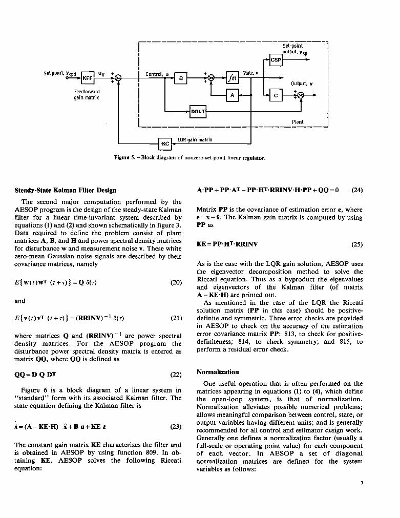
LQR gain matrix 1 Figure 5. -Block diagram of nonzero-set-point linear regulator.

Steady-State Kalman Filter Design

The second major computation performed by the AESOP program is the design of the steady-state Kalman filter for a linear time-invariant system described by equations (1) and (2) and shown schematically in figure 3. Data required to define the problem consist of plant matrices A, B, and H and power spectral density matrices for disturbance w and measurement noise v. These white zero-mean Gaussian noise signals are described by their covariance matrices, namely

and

E(v(t)vT ( f + ~ ) ) =(RRINV)” 8 ( ~ ) (21 1

where matrices Q and (RRINV)-’ are power spectral density matrices. For the AESOP program the disturbance power spectral density matrix is entered as matrix QQ, where QQ is defined as

A-PP + PP*AT- PP*HT*RRINV*H*PP + QQ = 0 (24)

Matrix PP is the covariance of estimation error e, where e = x - f. The Kalman gain matrix is computed by using PP as

As is the case with the LQR gain solution, AESOP uses the eigenvector decomposition method to solve the Riccati equation. Thus as a byproduct the eigenvalues and eigenvectors of the Kalman filter (of matrix A - KE-H) are printed out.

As mentioned in the case of the LQR the Riccati solution matrix (PP in this case) should be positive- definite and symmetric. Three error checks are provided in AESOP to check on the accuracy of the estimation error covariance matrix PP: 813, to check for positive- definiteness; 814, to check symmetry; and 815, to perform a residual error check.

Q Q = D Q DT (22) Normalization One useful operation that is often performed on the

Figure 6 is a block diagram of a linear system in matrices appearing in equations (1) to (4), which define “standard” form with its associated Kalman filter. The the open-loop system, is that of normalization. state equation defining the Kalman filter is Normalization alleviates possible numerical problems;

allows meaningful comparison between control, state, or

k=(A-KE.H) i + B u+KE z output variables having different units; and is generally (23) recommended for all control and estimator design work.

Generally one defines a normalization factor (usually a The constant gain matrix KE characterizes the filter and full-scale or operating point value) for each component is obtained in AESOP by using function 809. In ob- of each vector. In AESOP a set of diagonal taining KE, AESOP solves the following Riccati normalization matrices are defined for the system equation: variables as follows:

I

r- ””“””“””“”” 1 I

I i i i i L,

r i I 1 I

I

t I Measurement, z

i I

-

I

Plant

“””“” +- ”““_ I

I I

Kalman Filter I L ”“”“””””- I Figure 6. -Block diagram of open-loop system with Kalman filter.

SCY SCYSP

The normalization (scale) factors SCX, etc., can be considered to be diagonal matrices but are stored in AESOP as single-dimensioned arrays. Function 404 is provided in AESOP to normalize all of the matrices that define the system and the control and estimation problems, namely: A, B, C, D, DOUT, CSP, QQ, and RRINV. As an example of the calculations performed, consider the normalization of the CSP matrix. We have that

ysp = CSP x (26)

Explicit definition of the normalization factors for x and ysp are given by

Ysp 4 SCYSP Gsp (27)

x e s c x x (28)

8

where the overbar indicates the normalized vector. Thus the normalized CSP matrix (call it WP) can be obtained as

SIsp = csp x (29)

where

- CSP = (SCYSP) - ‘*CSP.SCX (30)

The other matrices are normalized in a similar manner. Note that performance index weighting matrices QC, NN, and PCINV are not normalized in AESOP because they are considered to be “free” parameters to be manipulated by the designer. For example, “Bryson’s rule,” the often-used rule of thumb for choosing starting values of QC and (PCINV)-’ states that the matrices should be diagonal, where each diagonal term is simply 1 divided by the square of the maximum (or operating point) value of the corresponding state or control variable. If the system is normalized, the same result can be obtained by simply making QC and PCINV identity matrices.

If normalization is used before conducting LQR or Kalman filter designs, it may be desirable to have normalized gain matrices KC, KE, and KFF put back in dimensional form (unnormalized). Function 405 is pro-

vided in AESOP for this purpose. In addition, this function unnormalizes the error covariance matrix PP.

Stochastic Linear Quadratic Regulator Design

The solution of the linear quadratic regulator problem requires that the state vector x be completely measurable. In general, this will not be possible. Usually, only a vector of NM noisy measurements z, which are linearly related to the state x, will be present for use by the control. In line with the separation principle (ref. 12), the optimal control for this situation is constructed by feeding back an optimal state estimate (generated by a K h a n filter) through the optimal regulator gains KC. This system is optimal with respect to minimizing the stochastic equivalent of the quadratic performance index given by equation (12). That equivalent index is given by

J=E(xTQC x+2xTNN u+uT(PCINV)" u) (3 1)

AESOP provides the means for solving this optimal control problem by using the previously mentioned two functions for computing gain matrices KC and KE. The structure of the complete stochastic LQR problem is shown in figure 7. In addition to gain computations it is also of interest to compute various system responses to characterize the complete closed-loop system. Of particular interest in the case of the stochastic LQR

system are the values of the covariance matrices for the system state, control, and output vectors. This is discussed in the following section.

System Response to Noise Inputs

The primary way to evaluate the overall performance of a system controlled by a stochastic linear quadratic regulator (such as is shown in fig. 7) is to examine the mean square or rms values of the various system variables. More generally, the quantities one wishes to compute are the covariance matrices for system vectors x, 2, u, z, and y. In particular, the mean square values are the diagonals of the covariance matrices. The two covariance matrices are XX, the covariance of the state vector x, and PP, the covariance of the Kalman filter estimation error e. As was mentioned previously, matrix PP is computed by AESOP function 809, which conducts the Kalman filter design. The second covariance matrix, XX, is obtained by solving the following Lyapunov matrix equation (ref. 12):

(A - B*KC)XX + XX(A - B.KC)T

+ B-KC-PP + PP*KCT-BT + QQ = 0 (32)

AESOP uses an iterative method developed in references 13 and 14 to solve this equation. In comparison

Set po in t

""""""""""" 1

Set-point output, ys I j Disturbance, I *-:Noise. v I,,- Measurement, z

Y S

"- "" """""""-

Figure 7. -Stochastic LQR block diagram showing plant, Kalman filter, LQR gain matrix, and feedforward gain matrix.

9

with other techniques this method has been found to be the error matrix, and (3) computes an average error value especially effective for cases where system order N is as Trace (E)/Trace (X). large (50 to 100).

function 817. Also, this function computes three other Response Calculations The Lyapunov solution is computed in AESOP Transfer Functions and Frequency

system covariance matrices, all simple functions of XX and PP. They are

(1) The covariance matrix of control u,

UU = KC*(XX - PP).KCT (33)

(2) The covariance matrix of measurement component 21 2

ZZ = H*XX.HT (34)

(3) The covariance matrix of output y,

YY = C.PP*CT+ (C - DOUTeKC)

.(XX - PP).(C - DOUT-KC)’ (35)

Note that covariances XX, UU, ZZ, and YY can be computed for cases where either (1) no control is used (open-loop response) or (2) no Kalman filter is used (state feedback only). The open-loop case can be computed by simply calling function 817 without first computing either PP or KC (these two matrices will thus be all zeros). The state feedback case can be computed by first calling function 801 to obtain KC and then calling function 817.

In addition to solving Lyapunov equation (32) for the state covariance matrix, AESOP has an error check function (number 818) that gives information on the accuracy of the solution. Consider a general Lyapunov equation

It is often quite useful to examine the characteristics of a state-variable system, either open or closed loop, in the frequency domain. For instance, one may wish to analyze the pole-zero structure of the system transfer function matrix, given a state-variable system description. For this purpose, one needs to be able to compute transfer function poles, zeros, and gain given the system matrices. As another example, one may examine the transfer function matrix of an optimal feedback controller to see if any simplifying pole-zero cancellations exist such that a lower order approximation can be made. Here too it is desirable to compute poles and zeros from a state-space description. Frequency response plots (for example, Bode plots) may be desirable so that one can evaluate, using classical frequency domain criteria, the response of a control system that was designed by using LQR methods. Or, given a state-space, open-loop system description, one may wish to compute a matrix of system transfer functions or a matrix of frequency responses that can subsequently be used by a frequency domain control design program. For these reasons, it was decided to include in AESOP the capability to compute transfer functions and frequency responses for various systems and subsystems defined in state-space terms.

Consider the generalized nth-order system described by state equations

A X + X AT+W=O (36) and having “nc” inputs u and “no” outputs y. These equations could represent any linear system (open-loop

Let the actual computed solution to equation (36) be x - plant, Kalman filter, closed-loop regulator, etc.) by Substituting X into equation (36) for X we obtain appropriate choice of vectors %, f , and ii and matrices A,

B, e, and D. The transfer function matrix G(s) relating A % + % A T + W = R (37) output vector f to input vector ii can be written as

where R is a residual matrix. Define an error matrix E e X - X . Subtracting equation (36) from equation

f(s) =[C(sI-A)”B+D]u(s) =G(s)a(s)

(37), we obtain another Lyapunov equation AESOP allows the user to obtain solutions to equation

transfer function G,(s) relating a component uj(s) to a component yi( s) in two forms.

AESOP function 818 uses matrix XX obtained from the The first transfer function form computed is where Lyapunov solution of function 817 and (1) solves for the each G,(s) is a ratio of polynomials. In this case the residual matrix, (2) solves a Lyapunov equation to obtain general expression for G;ii(s) is

A E + E AT-R=O (38) (41) for a variety of system configurations. It computes a

10

I ” I k= 1 G,(s) = ”

Note that since a feedforward matrix D is assumed, G;ii(s) may have equal-order (n) numerator and denominator. AESOP uses the technique of reference 15, modified slightly to include a D matrix, to compute coefficients ak and bk. Constants bk are the coefficients of the characteristic equation of and are thus common to all G;ij(s).

The second transfer function form computed by AESOP is the so-called factored form, where the general expression is given as

m

G i j ( s ) = (43 1

k = 1

where Zk and P k are the transfer function zeros and poles, respectively. In addition to poles and zeros, AESOP computes gains Kg and the number of numerator zeros m (m In). The poles P k are obtained in AESOP simply as the eigenvalues of A. The method for obtaining m and zk depends on the value of Dg.

For cases where Do is equal to zero the values of m and Zk are obtained by using a method developed by Davison (ref. 16). The method is essentially based on a concept from root locus theory. That is, if a proportional loop is closed between output f i and input ii, and the loop gain is allowed to increase to infinity, m of the root loci (poles of the closed-loop transfer function) will go to the m open- loop transfer function zeros, and the remainder (n -m) will go off to infinity. Davison’s method successively computes the eigenvalues of such a system while increasing the loop gain. It stops when the n -m “extraneous” eigenvalues all exceed a “large” value.

For cases where the value of D, is nonzero, the number of zeroes and poles of the transfer function G;ij(s) are both equal to n. In this case the zeroes are simply the eigenvalues of the matrix

where

This fact can be seen by applying a feedback control

6 .- - keyi J - (45)

to the system of equations (39) and (40) and allowing gain k* to go to infinity. In the limit the eigenvalues of A* become the zeros of the transfer function G;ij(s).

The remaining transfer function term in equation (43) to be computed is gain Kg. AESOP uses the technique described by Brockett (ref. 17) to compute this gain as

Computations for two types of transfer functions, polynomial form and factored form, are performed in AESOP series 500 and 700, respectively. System configurations for which calculations are done are (1) an open-loop system, (2) a system with state feedback, (3) a system with a Kalman filter in the feedback loop, and (4) an optimal controller. Polynomial-form transfer function coefficients are computed for the purpose of plotting frequency responses. The AESOP program uses the same subroutines to compute frequency responses and transfer functions for each configuration, first forming the appropriate A, B, e, and D matrices as functions of A, B, KE, KC, etc. Factored-form transfer function information (poles, zeros, and gain) is mainly of interest in one of two instances: (1) when investigating the structure of the open-loop system, and (2) when examining the pole-zero structure of an optimal controller. Therefore data are obtained by AESOP only for these two configurations. Frequency responses, however, are obtained for all four configurations mentioned previously. Table VI1 in the next section outlines in detail which calculations AESOP does perform.

Figure 8 shows the open-loop configuration for which transfer functions and frequency responses can be calculated. Corresponding to the form of equation (41), the four transfer functions that AESOP computes here are

11

Disturbance, w "m Control, u State, x

I

I Figure 8. -Block diagram of open-loop system for which transfer functions and frequency responses are obtained. Inputs are u and w; outputs

are 21 and y.

Control to output:

Y(S) =[(sI-A)" B+DOUT]U(S) (47)

Disturbance to output:

y(s) = C ( s I - A ) " D W(S) (48)

Control to measurement:

Z(S) = H ( s I - A ) - ' B U ( S ) (49)

Disturbance to measurement:

Figure 9 shows the second configuration -a system with state-variable feedback. Here AESOP computes the following frequency responses by using disturbance w as the input:


y (s) = ( C - DOUT.KC)[(SI - (A - B*KC)] - D w (s)

(51)

Disturbance to control:

U(S) = -KC[sI-(A-B-KC)]" D W(S) (52)

Disturbance w is not explicitly used in the design of the (noise free) linear quadratic regulator (e.g., eq. (14)). However, it is instructive to examine its disturbance response in the frequency domain.

Figure 10 depicts the configuration where disturbance w is explicitly considered in the control system design, namely the stochastic linear quadratic regulator. The overall system order in this configuration is 2N, there being N states x and N state estimates 2. In obtaining frequency responses AESOP first forms partitioned system matrices before calling the subroutine that computes the responses. The following responses are computed:


Control, u r

i """""""""""" 1

I i ! output, y I * I

I I

I DOUT h' I

i _"" -"I Plant i LQR gain matrix "

Figure 9. -Block diagram of LQR configuration used for obtaining frequency responses input is w; outputs are y and U.

12

I I i I

i 4

i I I DOUT] I I L "" 1 """""""" i

I i I i

i

Plant J Control, u LQR gain matrix -

"""""""""- - Kalman filter 1

%

I

I

'rState estimate. I -

W f I I

I i Kalman filter J Figure 10. -Block diagram of stochastic LQR configuration used for obtaining frequency responses. Input is w ; outputs are y. z , and u.

Y (s) = CTOT (SI - ATOT) - DTOT w (SI

Disturbance to measurement:

Z(S) =HTOT(SI-ATOT)-~ DTOT W ( S )

Disturbance to control:

u ( S) = KCTOT (SI - ATOT) - DTOT w (S )

where

- B-KC

DTOT= - - - - , 2 N X N D 1 CTOT = [C I - DOUT*KC], NO X 2N

HTOT=[H IO], NMx2N

KCTOT=[OI -KC], NCx2N

Note that measurement noise, although a consideration in the Kalman filter design, is not considered here as an input.

The last configuration for which frequency responses as well as transfer function zeros and gain is computed is the optimal controller, shown in figure 11. This is simply the feedback portion of the control loop of figure 10, the stochastic regulator. The desired response is for measurement z as an input and control u as an output. This transfer function can be expressed as

u (s) = - KC[SI - (A - B-KC - KE'H)] - KE Z(S) (56)

It has been noted in the literature that this optimal controller transfer function can have some interesting properties; for example it can sometimes be unstable (ref. 18) or can have right-half-plane zeros (ref. 1).

Transient Response Calculation

The AESOP program computes and plots transient responses for several important system configurations. Consider again the general time-invariant system, which is described in state-variable form as

% ( t ) = A W ( t ) +B h ( t ) (57)

f ( t ) =c W ( t ) + D h ( t ) (58)

13

Control. u LOR gain matrix

"""""" ---""

i Kalman filter I I ,-State estimate, ii

I I

Meaprement, z

I i L """"""""- Kalman filter i

Figure 1 1 . -Optimal controller, comprising Kalman filter and LQR gain matrix. Input is measurement z and output is control u.

In AESOP it was desired to solve these general equations (1) Open-loop system -The equations for this system, (57) and (58) for two cases: (1) an initial condition %(O), shown in figure 3, are and (2) a step change in input ti ( t ) . The normal approach, and that taken in AESOP, is to discretize X= A x + B u (65) equation (57) so as to obtain the exact solution at time points to, t l , . . ., t k that are spaced DT seconds apart. y = C x + DOUT u (66) The resulting discrete difference equations are thus

AESOP calculates and plots x and y for ITRMX time

(59) points for either

(a) A step input applied to component i of input

(60) u ( t ) (b) An initial condition x(0) on the ith component of

the state vector x ( t ) . These computations are performed by AESOP functions

(61) 601 and 602, respectively. (2) Closed-loop linear quadratic regulator -Figure 4

(62) shows the configuration of this system. The describing equations are

and matrices I@ and r are given by the series representations

and

A-DT2 A2.DT3 +

= (,.,,, - + ~ 2! 3!

. .

X= (A - B-KC) X (67)

y = C x+DOUT u (68)

Matrices A, B , e, and D are appropriately formed by AESOP and variables x, y , and u = - KC x are calculated and plotted. This is done for an initial condition xi(0) on a selected component of x(0). Function 603 accomplishes these calculations. The responses for x, y , and u can be compared by the user with the open-loop responses in order to help evaluate a particular LQR design.

(3) Nonzero-set-point linear quadratic regulator -This system, shown in figure 5, is described by one state and three "output" equations:

(63)

. . )B (64)

X = (A - B-KC) X + B*KFF Yspd (69) Matrix r is computed by assuming that input ti( t ) is constant over t, st < t , + 1. The series in equations (63) Y = (c - DOUT-KC) x + D 0 U T . m Yspd (70) and (64) are carried out until the desired accuracy in + and r is achieved. ysp = CSP x (71)

The general procedure just described is used to compute transients for the following three situations: U = - K C X + m y S p d (72)

14

Here again, AESOP forms the appropriate matrices before computing the responses. The response of interest here is to a step change in a selected component of the set- point vector Yspd. Of interest to the user in this configuration are such things as rise time and overshoot of the kth component of ysp in response to a step change in the kth component of Yspd; interaction -the response of the kth component of ysp to a change in the ith component of Yspd; and the magnitudes of control variable excursions. The computation and response plotting for the nonzero-set-point regulator are performed by AESOP function 604.

AESOP Program Operation This section provides an overview of how to operate

the AESOP program. In particular, it discusses how the user interfaces with the program within the IBM 370 TSS PCS (Program Control System) environment, how to enter data, how to enter a string of control numbers that dictate the series of AESOP functions to be performed, and in general, how the user interfaces with the program at the “terminal,” not Fortran, level. (It is assumed that the reader is familiar with PCS commands and the operation of the 370 TSS system.)

Program Structure

The general structure and operation of AESOP was described in the Introduction and shown schematically in figure 1. A more detailed diagram of the program showing the main AESOP program and nine main subroutines is given in figure 12. Each main subroutine contains a number of related AESOP functions. The numbers above the main subroutine boxes in figure 12 indicate the function series that each main subroutine contains (800 contains functions 801 to 899, etc.). The details as to what each function does will be discussed later in this section.

Main subroutines

Program control

h M I

All input and output performed by the main AESOP program relate to program control and required interfacing with the user. The main program (1) initializes default or reference values, (2) accepts a string of function numbers that the user wishes to have performed, (3) performs checks to see whether the user has requested functions to be done in a reasonable order, and (4) calls the appropriate main subroutines in which the desired functions reside.

To run the AESOP program, the user first calls the PROCDEF (for PROcedure DEFinition) AESRUN, defined in appendix D. Through use of TSW370 datadef (DDEF) statements, AESRUN

(1) Defines (“datadefs”) the library dataset (file) that contains the compiled AESOP program and all subroutines and then loads the program

(2) Defines the link to the graphics package that contains graphics subroutines called by AESOP

(3) Links (“datadefs”) Fortran unit numbers with specific dataset (file) names so that these files can be written to or read from during the subsequent AESOP run AESRUN has a single parameter that is used to identify all output datasets to be generated during the AESOP run. After calling AESRUN, the user types “AESOP” to run the program.

Operating Procedure

The key element in the use of AESOP is the single- dimensioned function number array (Fortran symbol IFN). The user loads, in sequence, this vector with the numbers of the AESOP functions that are to be performed. The use of the IFN vector and the general operation of AESOP will be explained with the aid of the flow chart of figure 13. The user many also refer to the terminal listing included in appendix C for test case I for an actual example of how AESOP is run. First, the user types “AESRUN” followed by its parameter. The

AESOP

I

Matrix formation

Open-loop system

I Transient I I Transfer 1 1 :::fz/and I I User-supplied 1 responses functions filter design subroutines

Figure 12. -AESOP program structure.

15

I AESRUN [I. D. PARAMETER] I

Heavy blocks indicate occurrence of prompts or terminal responses

ON-LINE PLOTS. Y OR N? IONPLT = 1

P R EQUAL TO a,CHARACTERS)

ENTER THE PARAMETER YOU USED FOR AESRUN

1 . T I

EXTENDED TERMINAL OUTPUT? I P R T = 2

DDEF 21 TO THE

I 4 ENTER NAMELIST NI DATA (IFNIJ I

r“F“ M Z = 0

Figure 13. -Flow chart for AESOP program.

computer responds with information that the libraries have been set up and all datasets have been datadeffed. The user then types “AESOP” to call the main program. (Note that the heavy blocks in figure 13 indicate either user input commands or messages printed out at the user’s terminal.) The program then responds by prompt- ing the user with the message:

DO YOU WISH TO MAKE PLOTS, Y OR N?

If the response is “Y,” the user is then asked to

ENTER THE PLOT NAME - 8 ALPHANUMERIC CHARACTERS

16

This name will be used to name the plot dataset in which any plots generated will be stored. Next, the user is asked,

DO YOU WISH TO MAKE ON-LINE PLOTS, Y or N?

If the reply is “Y,” the program sets an internal flag that will cause the program to PAUSE after each on-line plot is displayed to allow the user to view it. Off-line plotting requires no such action to be taken. Finally, the user is asked for two pieces of information that will appear on all plots for identification purposes:

ENTER TODAY’S DATE (LESS THAN OR EQUAL TO 20 CHARACTERS)

I -1s IFN(MZ) the ntmber of a n executable FCN?% . ._

Prerequisite error

1 I check I

I YOU HAVE NOT EXEC- UTED THE FOLLOWING PREREQUISITE FUNCTIONS

t t THESE ARE THE FUNCTIONS YOU HAVE RUN THUS FAR. THE PRESENT FUNCTION I S NOT A LEGIT1 MATE ONE. YOU WILL NOW HAVE A CHANCE TO REPLACE I T WITH ONE GOOD ONE, TO TERMINATI OR TO CENTER A LIST OF FUNCTIONS. TYPE Y TO ENTER ONE REPLACEMENT FUNCTION; TYPE N TO ENTER A LIST OF FUNCTIONS

.)

TO COMPUTE FURTHER, ENTER IFNII3), ONE PER 0 REPLACE THE CURRENT LINE; TO TERMINATE, FUNCTION; I F THE NUMBE ENTER 999 (LAST ENTRY I S 999, THE PROGRAM MUST BE A RETURN)

Read new function Read IFN(MZ) number into IFN

DDEF NAME OF N1 DATASET to 21 h

I I I + + J

End

Figure 13. -Concluded.

and provided as part of AESOP. Thus the preceding messages and prompts would be tailored by each user to reflect the

ENTER THE PARAMETER YOU USED FOR specific graphics package being used. AESRUN After the graphics-oriented prompts are handled, the

In view of the fact that graphics subroutines are rather specific to the user’s computer system, they are not EXTENDED TERMINAL OUTPUT?

program displays the message

17

(This question and all subsequent ones are to be answered “Y” (yes) or “N” (no). All output produced by the program is stored on the output dataset, which the PROCDEF AESRUN datadeffed to unit 06. Two subsets of this output are available for display on-line at the user’s terminal. The EXTENDED TERMINAL OUTPUT option (appendix D) allows the user to view a more extensive subset of data if desired.

Next, the user is prompted with the message

READ IN N1 FROM STORAGE?

The N1 referred to here is the name of a Fortran NAMELIST that contains the vector IFN. For problems that are solved over and over again, using the same AESOP functions but different data, it is convenient to store the NAMELIST N1 in a dataset to avoid having to type it each time at the terminal. If this is the case, the user would respond with “Y” and the program would print out

DDEF 21 TO THE N1 DATASET

At this point the user would then type the required datadef statement, for example,

DDEF FT21FOOl,VS,MYNlDS

where dataset MYNlDS would contain typical NAMELIST data such as

&N1 IFN=201,701,999 &END

However, to enter a new set of numbers into the IFN vector, the user would enter “N” and the program would respond with

ENTER NAMELIST DATA AS ’&N1 IFN = , , , &END

At this point the user would type a NAMELIST N1, such as was given in the preceding example.

The IFN string can be terminated in two ways. If the user ends it with a number greater than or equal to 999 (as was done in the preceding example), the AESOP program will execute all of the requested functions and then terminate the run. (The number 999 is a request for termination.) If the user ends the string with the number of an executable function, the program will allow more function numbers to be entered when the present string of functions has been executed. In either case, as soon as the NAMELIST has been read by the program, the program displays all of the elements of the IFN vector at the terminal and starts to execute the requested series of functions.

Figure 13 shows that the main program indexes integer MZ each time just before it begins to execute a function. This integer denotes the element of the IFN vector that contains the number of the function about to be executed. The program then performs four successive checks on IFN (MZ), the MZth element of IFN. These checks are

(1) Is the IFN(MZ)2999? If so, terminate the program; if not, continue checking.

(2) Is IFN(MZ) I 100 but not equal to zero? If so, you have requested a nonexisting function and will be allowed to change the requested number.

(3) Is IFN(MZ) = O? If so, you have reached the end of the function number string requested and will now be able to enter additional function numbers if desired.

(4) Is IFN(MZ) the number of an existing executable function in series 100 to 900? If so, the function will be executed; if not, you will be allowed (as in check (2)) to change the requested number. As an example, first, assume that the present IFN(MZ) encountered is a nonexisting function number (i.e., checks (2) or (4) above were failed). The program displays the messages

THESE ARE THE FUNCTIONS YOU HAVE RUN THUS FAR nnn THE PRESENT FUNCTION IS NOT A LEGITIMATE ONE, YOU WILL NOW HAVE A CHANCE TO REPLACE IT WITH ONE GOOD ONE OR TO

TIONS. TYPE Y TO ENTER ONE REPLACEMENT FUNCTION; TYPE N TO ENTER A LIST OF FUNCTIONS

TERMINATE OR TO ENTER A LIST OF FUNC-

If the user types “Y,” the program responds with

TYPE IN AN I3 NUMBER TO REPLACE THE CURRENT FUNCTION; IF THE NUMBER IS 999, THE PROGRAM WILL TERMINATE

The user would then enter a new function number and the program would repeat the four checks. If the new number is that of an executable function, the program proceeds to execute the function.

If the user types “N” in response to the previous prompt, the program will display the message

TO COMPUTE FURTHER, ENTER NEXT FUNCTION NOS. (I3), ONE PER LINE; TO TERMINATE ENTER 999 (LAST ENTRY MUST BE A RETURN).

The user may then enter a series of function numbers, hitting “RETURN” after each three-digit number and

18

hitting “RETURN” twice after entering the last number in the series. The program also responds with the preceding prompt whenever it encounters IFN(MZ) = 0, which is the indication that the end of the previously requested function string has been reached.

The previous paragraphs have dealt with situations where the program detects nonexistent function numbers in the input string. In the case where the function number is correct, the main AESOP program then calls the appropriate main AESOP subroutine in which the function resides. At that point a prerequisite check is begun. As a user aid the AESOP program contains a table of prerequisite functions (appendix F). The program checks the prerequisite table immediately before executing each requested function to insure that the specified prerequisite functions have already been performed. For example, suppose the user enters function number 401, which requests that open-loop eigenvalues (of the A matrix) be computed, without preceding this number with either number 201 or 202, the functions that form or read in data that define the system. Just before calling function 401 the program checks the prerequisite table and detects that the proper prerequisites (either function 201 or 202) have not been performed prior to this function. The program then displays the message

YOU HAVE NOT EXECUTED THE FOLLOWING PREREQUISITE FUNCTION(S) FOR FUNCTION 401

and then prints out pertinent function numbers. It then displays the message

IF YOU THINK YOU KNOW WHAT YOU ARE DOING AND WISH TO IGNORE THE PREREQS AND CONTINUE ON TO DO THIS FUNCTION, TYPE Y AND RETURN; OTHERWISE, JUST RETURN

The prerequisites in the table for each AESOP function were selected so as to catch most, if not all, errors a user might make in selecting a series of interdependent functions that could lead to calculations that would produce major errors. These would be errors such as zero divides during inversion of a singular matrix, etc. It was felt that protecting against these nuisance errors would make it less likely that a user would have to restart the program in midcourse because of a major nonrecoverable error. However, it is still possible to select a series of functions that produce nonsensical results even though prerequisite checks show no error.

To terminate the program, the user types “999” when the program asks for more function numbers. The program will then display the message

STORE THE Nl FOR THIS RUN?

This allows the user to store the IFN vector, which was just used in the present run, on a dataset for possible future use. If this is desired, the user replies with “Y” and will receive the message

DDEF NAME OF N1 DATASET TO 22

The user would execute the required datadef, using whatever dataset name was desired, and then type “GO” to cause the program to terminate. If the IFN array is not to be stored, a previous response of “N” would terminate the run immediately.

Data Input and Output

A key aspect of the AESOP program is the handling of data input and output. The primary input and output device is the user’s terminal. Most of the data sent or received through the terminal pertain to program control, as was demonstrated in the examples in the previous section. That section also showed two examples of how the program accesses data that are stored in a dataset (IFN, read from unit 21) and how the program writes data out to a dataset (writing IFN onto unit 22). In the program, however, 14 unit numbers are used for input and output of data (in addition to unit 02, reserved for the terminal, and unit 06, reserved for the high-speed printer output). All units are listed in table I together with the names, contents, and format of their associated datasets. Dataset names are created by the PROCDEF AESRUN, which appends the characters in parameter $1 to an identifying prefix. For example, referring to table I, if the parameter $1 were entered as XYZ, the PROCDEF would datadef unit 08 to dataset CGXYZ. This dataset is the one in which the control gain matrix KC is stored. Other datasets that are identified by using the parameter $1 are those datadeffed to unit 09 (containing the Kalman filter gain matrix), units 10 to 14 (containing frequency response magnitudes and phase angles), unit 15 (estimation error covariance matrix), unit 16 (control Riccati equation solution matrix), and unit 17 (feedforward gain matrix). The remaining units, 33 and 34, are for datasets that store the data that define the design problem to be solved by AESOP, namely the open-loop plant data (unit 33) and normalizing factors (unit 34). The user must datadef these units and specify the names of their associated datasets.

Much of the input data for AESOP is in NAMELIST form. Table I1 lists all NAMELIST’s used by the program and the names of the Fortran variables contained in each. A key NAMELIST is MATDAT, which contains all matrix coefficients and dimensions needed to define the problem to be solved. NAMELIST’s CONPAR and ESTPAR, which are useful when modifying basic problem data, contain subsets of the variables contained in MATDAT. CONPAR is used for

19

Un i t

-

02

08 06

09 10

11 12 13 1 4 15

17 16

21 22 33 34

Dataset name

""_" OUTBla

CGQ1 EG$l

PFRUZ81

PFRUYBl PFRWZ$l PFRWY$l

CFR51 PPQl SS81 FFGSl (b) (b) ( b ) (b)

I m L t I. - U H I H ~ ~ I ~ HNU UNIIJ uxu ~ U K Y K U ~ K H M IIYYUI HIYU u u I r u I

C o n t e n t s o f d a t a s e t ~ " ~

. . -

All t e r m i n a l i n p u t and o u t p u t

KC, c o n t r o l g a i n m a t r i x H igh -speed-p r in te r ou tpu t

KE, Kalman f i l t e r g a i n m a t r i x Frequency response, z( IMEAS)/u( JINC)

Frequency response, y( IOUT)/u(JINC) Frequency response, z ( IMEAS) /w( JIND) Frequency response, y(IOUT)/w(JIND) Frequency response, u( J I N C ) / z ( IMEAS) PP, e s t i m a t i o n e r r o r c o v a r i a n c e m a t r i x SS, c o n t r o l R i c c a t i s o l u t i o n m a t r i x KFF, f e e d f o r w a r d g a i n m a t r i x I F N v e c t o r , c o n t a i n e d i n NAMELIST N1 IFN vec tor , con ta ined i n NAMELIST N 1 Open-loop p l a n t d a t a , NAMELIST'S MATDAT and REFS Vorma l i z ing f ac to rs ; NAMELIST NRMS

"" . .

1 Format I

Var ious

Unformat ted Var ious

I

V NAMELIST

Funct ion where r e a d / w r i t t e n

Many Many

205/802 206/810

.. .

"""""""

"""""""

"""""""

208/816

209/820 207/808

Main program Main program

202 404 and 405 "~ "" -

"_ Comments

Te rm ina l i npu t and ou tpu t

See t a b l e VI f o r d e t a i l s on f requency responses

""""""""""-"""-

F o r i n p u t o f I F N F o r o u t p u t o f I F N Usua l source o f p rob lem da ta """"""""""""""

a $ l i s t h e p a r a m e t e r f o r PROCDEF AESRUN; it serves as an a r b i t r a r y i d e n t i f y i n g t a g ( f e w e r t h a n f o u r c h a r a c t e r s ) f o r t h e

bUser spec i f i ed . naming o f d a t a s e t s ) .

TABLE 11. - NAMELISTS USED I N AESOP PROGRAM -~ . ~.

NAMELIST . . ~

CONPAR

ESTPAR

MATDAT

NRMS

N 1

REFS

V a r i a b l e s i n NAMELIST

QC, NN, PCINV

QQ, RRINV

A, 6 , C , 0, H, DOUT, CSP, QC, NN, PCINV, QQ, RRINV N, NM, NC, NO, NO

SCX, scu, SCY, scz, SCYSP

IFN

TSFTR, OT, F I , DELF, ZERMAX, 4MPSP, AMPSR, AMPICX, IF, ISPACE, IOUT. ~ IMEAS. -JINC. JINO. -ITRMX. UCURV, LINLOG, MSPY, MSPYSP, '

rlSPU, MSROLY, MSROLX, MICCLY, UIICCLX, MICCLU, MICOLY, MICOLX

making changes in performance index weights, and ESTPAR is used for varying noise matrix elements.

NAMELIST NRMS contains normalizing factors whose use is described by equations (26) to (30). The remaining NAMELIST, REFS, is used for setting various parameter values that specify such things as time steps, frequency point spacing and numbers, perturbation amplitudes, and input and output selection indices. Table I11 specifies each parameter in REFS and its default value and indicates in which AESOP function each parameter is used. For a more detailed explanation of each parameter, refer to the appropriate function description given in the next section.

20

I npu t sou rce ~ ".

- . .

Termina l

Terminal

T e r m i n a l o r d a t a s e t

Oataset

Termina l

Te rm ina l o r da tase t

"" ~~ . . .

Comments ~ .. ~~ .

r e a d i n f u n c t i o n 203 F o r r e v i s i n g w e i g h t i n g m a t r i c e s ;

F o r r e v i s i n g n o i s e power s p e c t r a l d e n s i t i e s ; r e a d i n f u n c t i o n 204

P r i m a r y means o f e n t e r i n g s y s t e m

changed i n f u n c t i o n 210 data; read i n f u n c t i o n 202;

r e a d i n f u n c t i o n 404 o r 405 C o n t a i n s n o r m a l i z i n y f a c t o r s ;

P r o g r a m c o n t r o l ; r e a d o r w r i t t e n i n main program

See t a b l e I11 f o r d e f i n i t i o n o f a l l v a r i a b l e s and d e f a u l t v a l u e s ; s e t i n main program; change i n f u n c t i o n 101; r e a d i n f u n c t i o n 202

". . . "

Description of AESOP Functions

Each AESOP function will now be described in sufficient detail so that this section can serve as a primary reference when using the program. All functions, as indicated previously, are grouped into nine series (series 100 to 900). When possible, a general description will be provided for each series, with an accompanying table included to show similarities and differences among functions within the series. Also, whenever possible, the reader will be referred to appendix C, test case I, for an example of the use of each function.

TABLE 111. - DEFINITION OF PARAMETERS CONTAINED I N NAMELIST REFS

V a r i a b l e

DT

ITRMX AMPSR AMPSP AMPICX MSROLYa MSROLXa MICOLYa M ICOLXa MICCLYa M ICCLXa M ICCLUa MSPYSPa MSPYa MSPUa

F I DELF NCURV

L INLOG

I F ISPACE TSFTR

IOUT

IMEAS JINC JIND

ZERMAX

Gimension

Sca lar

S c a l a r NCMAX NCMAX NMAX NCMAX~, NOMAXC N C M A X ~ , NMAXC N M A X ~ , NOMAXC N M A X ~ , NMAXC N M A X ~ , NOMAXC

N M A X ~ NCMAXC NCMAX~, NCMAXC N C M A X ~ , NOMAXC NCMAX~, NCMAXC

Sca la r

NMAXb, NMAXC

Sca lar

Sca la r

D e f i n i t i o n D e f a u l t v a l u e

Time s tep 0.05 sec

Desired maximum number o f t ime s teps Open-loop system s tep inpu t ampl i tude vec tor All e lements a re se t to 1.0

I n i t i a l - c o n d i t i o n a m p l i t u d e v e c t o r All elements a re se t to 1.0 I n p u t l o u t p u t s e l e c t i o n m a t r i x All elements a re se t to 1

Star t ing f requency fo r f requency responses Frequency-point spacing

= 1, c losed l oop on l y = 2, c r o s s p l o t open- and closed-loop responses;

= 1, l i n e a r Bode p l o t s ; = 2, l o g Bode p l o t s ; = 3, b o t h l i n e a r and l o g p l o t s

Desired number of f requency response po ints Every ISPACE f requency response po in t i s 1 i s t e d Time sca le f ac to r , used f o r i nc reased p rec i s ion

I n d e x f o r s e l e c t i n g component o f y v e c t o r

Index f o r s e l e c t i n g component o f z vec tor

Index f o r s e l e c t i n g component o f w v e c t o r Index f o r s e l e c t i n g component o f u v e c t o r

10 t imes va lue o f l a rges t expec ted t rans fe r f unc t i on ze ro

0.01 Hz 0.02 Hz

2

3

49 1

1.0

1

1 1 1

100 rad/sec

Functions where used

j e r i e s 600 ( t ransient responses); 'unc t ions 601 to 604

v Ser ies 500, frequency responses

It

Ser ies 500 (frequency responses) and se r ies 700 ( t r a n s f e r f u n c t i o n s )

I Ser ies 700

aSee t a b l e VI1 f o r d e t a i l e d d e s c r i p t i o n . ROW s ize . CColumn s ize .

When running the AESOP program, it has been found helpful to have available a brief list of all possible functions. This list is provided in tabie IV. Once the user has read this report and is generally familiar with what the program can do, table IV can be used as a ready reference guide while running AESOP. More specific details on the various functions are given here.

Series 100 - Program Control

Series 100 contains only two functions: one for changing reference parameter values, and the other to allow the user to change datadefs in the middle of a run.

101-Change reference values by using NAMELIST REFS. -Table I11 describes various parameters in NAMELIST REFS that are used in the AESOP program to determine time and frequency steps, input and output indices, etc. The table also gives the default values of these parameter values that are initialized in the main AESOP program. Function 101 allows the user to change any or all of these parameters. It prompts the user with the message

ENTER CHANGES TO NAMELIST REFS (TSFTR, DT, FI, DELF, ZERMAX, AMPSP, AMPSR, AMPICX, IF, ISPACE, IOUT, IMEAS, JINC, JIND, ITRMX, NCURV, LINLOG, MSPY, MSPYSP, MSPU, MSROLY, MSROLX, MICCLY, MICCLX, MICCLU, MICOLY, MICOLX)

after which the user can enter the desired parameter changes. An example of the use of function 101 appears in appendix C, test case I, page 65.

102 -PA USE to allow user to change datadefs. - If the user requests this function, the program will display the message

YOU MAY NOW CHANGE YOUR DDEFS IF YOU WISH. DON'T FORGET TO CLOSE AND RELEASE THE OLD ONES FIRST

The program then effects a Fortran PAUSE and the keyboard unlocks to allow the user to make the appropriate changes. This function is useful, for example, when the user wishes to read in NAMELIST's MATDAT and REFS from dataset BBB, where previously similar data had been read from dataset AAA. At the requested PAUSE, the user can then enter

CLOSE AAA RELEASE FT33F001

and then

DDEF FT33F001,VS,BBB

and then type "GO" to continue execution. Subsequently, the user can request function 202, which will read in the desired data from dataset BBB.

Series 200-Data Input and Revision

This series of nine functions is used for inputting basic problem-defining data from datasets or for inputting changes to that data. The changes are typed in from the user's terminal.

201 -Forming matrices for test case I. - Function 201 is of use mainly when executing test case I , which is presented in appendix C. Function 201 simply forms all matrices and defines all dimensions, all of which are included in NAMELIST MATDAT. The specific matrices that this function forms for the test case are shown in table V. The dimensions for this problem are N=3, NC=2, NM=1, NO=2, and ND=2.

202 -Primary function for problem-defining data input. - Function 202 is the one usually used for reading in (from a VS dataset) the data that define the user's problem. The data must reside in the dataset in the following NAMELIST form:

&MATDAT (data for variables in NAMELIST

&END MATDAT - see table 11)

&REFS (data for variables in NAMELIST REFS -

&END see table 11)

Note that data for the two NAMELIST's must be in the order shown. It is not necessary to have any of the REFS parameters entered if the user wishes to have AESOP use the default values shown in table 111. However, the entry in the aforementioned dataset must then appear as

&REFS &END

203, 204, and 210- Functions used for revising data that define the user'sproblem. -Functions 203, 204, and 210 are useful when conducting design iterations, for filter design, regulator design, or plant sensitivity studies. Each function allows various parameter changes to be made via NAMELIST's from the user's terminal. (For NAMELIST definitions, see table 11.)

Function 203 is used to revise elements in the control design performance index weighting matrices QC, NN, and PCINV. NAMELIST CONPAR is used for this purpose. Function 204 is used to revise elements in noise power spectral density matrices QQ and RRINV through NAMELIST ESTPAR. These noise parameters, of course, strongly influence the characteristics of the associated Kalman filter. Function 210 is useful when changes are to be made in any of the variables in

22

TABLE IV. - SUMMARY OF AESOP FUNCTIONS

Funct ion Desc r ip t i on

:ompute 1 P l o t I S to re

Func t ion I D e s c r i p t i o n I Func t ion D e s c r i p t i o n

Program c o n t r o l T rans ien t func t ion zeros I Open-loop system ana lys i s Open-loop system:

702 701 u t o z

703 u t o y

704 w t o z

705 O p t i m a l c o n t r o l l e r w t o y

Func t ion Descr ip t ion

LQR, Kalman f i l t e r , and covariances

Change reference va lues Program pause

Eigenvalues

C o n t r o l l a b i l i t y , o b s e r v a b i l i t y , E igenvectors and mode shapes

and res idues Normal izat ion Unnormal izat ion

401

403 402

404 405

I I n p u t t i n g o r r e v i s i n g m a t r i c e s

M a t r i x i n p u t : M a t r i c e s f o r t e s t c a s e B a s i c m a t r i x d a t a i n p u t

Revis ing matr ices: QC, NN, and PCINV ( f o r LQR) QQ and RRINV ( f o r f i l t e r ) A, 6, C, DOUT, H, CSP, QC,

NN, PCINV, QQ, and RRINV

Reading s tored matr ices: KC ( f rom LQR) KE ( f r o m f i l t e r ) SS ( f rom LQR) PP ( f r o m f i l t e r ) KFF

201 202

203 204 210

205 206 207 208 209

Frequency responses I

Open loop: u t o z u t o y w t o z w t o y

With state feedback: w t o y w t o u

With Kalman f i l t e r feedback: w t o z

w t o u w t o y

O p t i m a l c o n t r o l l e r

503 506 509 512

525

502 505 508 511

514 516

518

522 520

524

501 504 507 510

513 515

517

521 519

523

- 801 508 802 805 806 807 -

809 Solve Riccat i equat ion 816 S to re so lu t i on ma t r i x SS/PP 810 Store ga in KC/KE 813 Check p o s i t l v e - d e f i n i t e n e s s o f SS/PP 814 Check s y m e t r y o f SS/PP 815 Compute r e s i d u a l e r r o r

Funct ion I D e s c r i p t i o n

Eigenvalues and e l yenvec to rs

803 E-values o f A - B*KC 811 E-values o f A - 6-KC - KE*H 812 E-values o f ATOT 804 E-vectors o f A - 6-KC

~~ ~~~ ~

M a t r i x f o r m a t i o n

n - B-KC R - B.KC - KE*H "Tota l " system matr ices

301 302 303

Transient response

601 602 603 604

Covariances, etc. Open-loop s tep Open-loop i n i t i a l c o n d i t i o n Closed-loop LQR i n i t i a l c o n d i t i o n Nonzero-set-point LQR s tep

817 Covariances o f LQR system 818 819

Covariance error check Feedforward ya in ca lcu la t ion (KFFJ

820 Store KFF

User-suppl ied subrout ines

901 UZR901 902 UZR902 903 UZR903 904 UZR904

TABLE V. - INPUT MATRICES FOR THIRD-ORDER TEST CASE

A =

1 2 3

B =

1 2 3

D =

1 2 3

C =

1 2

H =

1

I n p u t m a t r i x

1

-0.1000D-00 0.0000 0.0000

1

0.0000 0.0000

1.000

1

0.0000 0.0000

1.000

1

1 .ooo 0.0000

1

1.000

1

D.0000 3.0000

2

1.ooc 0.0000 -1.000

2

0.0000

0.0000 1.000

2

0.0000 1,000

0.0000

2

0.0000 1.0000

2

-

-~

I. 0000

2

I. 0000 1.000

3

0.0000 1.000

-0.20000-0

. .

3

I. 0000 1.000

3

).OOOO -

.~ . . . ~

-~

NAMELIST MATDAT, in particular, problem dimensions and matrices A, B, C, D, DOUT, H, and CSP. However, the noise matrices and the weighting matrices can be modified here also if so desired.

205, 206, 207, 208, and 209-Functions for reading gain and Riccati solution matrices. -AESOP contains three functions (801, 809, and 819) that solve Riccati equations and associated gain matrices and five functions (802,808,810, 816, and 820) that store results in datasets. Functions 205 to 209 are used for reading in datasets that contain gain or Riccati solution matrices previously computed by function 801, 809, or 819. Function 205 reads control gain matrix KC from dataset CG$l ($1 is the parameter in PROCDEF AESRUN). Function 206 reads Kalman filter gain matrix KE from dataset EG$l. Function 207 reads control Riccati solution matrix SS from dataset SS$1. Function 208 reads Kalman filter Riccati solution matrix PP from dataset PP$I. Function 209 reads feedforward gain matrix KFF from dataset FFG$l. Note that by using PAUSE function 102, the user can appropriately re-datadef any of the preceding datasets so as to read in the data from the particular dataset desired. Refer to table I for definition of the unit numbers associated with these five datasets.

Series 300 -Matrix Formation

The three functions in series 300 all take gain and open- loop plant matrices and form various matrices related to

24

i CSP =

1 2

QC =

1 2 3

NN =

1 2 3

QCINV =

1 2

99 =

1 2 3

lRINV =

1

.. ~ . .

.. .

I n p u t m a t r i x

1

1.000 0.0000

1

0.0000 500.0

0.0000

1

40.00 0.0000

32.00

1

0,0000 0.15630-01

1

0.0000

0.0000 0.0000

1

1.000

"

-

- ..

2

0.0000 0.0000

2

0.0000

0.0000 9.000

2

0.0000

0.0000 81.00

2

0.0000 0.12350-02

2

0.0000 2.000

0.0000

J

3

0.0000 2.000

3

0.0000 0.0000 0.40000-07

;..I 20.00

closed-loop control system configurations. Separate functions are assigned to forming these matrices because a number of AESOP functions require these same matrices as input. Table VI summarizes the three functions and indicates for which other AESOP function these three functions are prerequisites. Examples of using these functions are given in appendix C; for 301, pages 69 and 79; for 302 and 303, page 70.

Series 400 - Open-Loop System Analysis

This series of five functions is used in conducting pre- design analyses for the open-loop plant or for plant data normalization.

401 - Open-loop system eigenvalues. - Function 401 simply computes the eigenvalues of the A matrix. The eigenvalues are displayed in both Cartesian (a *j@) form and polar (frequency and {) where the frequency is in hertz and { is the damping ratio, { 4-cos(arctan I@~/CY). A negative 5' indicates a right-half-plane eigenvalue (or pair). An example appears on page 68 of appendix C .

402 - Open-loop eigenvectors and mode shapes. -Function 402 computes and prints out the modified eigenvector matrix for the A matrix and also these vectors in mode-shape form. Refer to the section Theoretical Background for a description of the modified eigenvector and mode-shape format. Note that one must call function 401 before calling function 402. Use of function 402 is also shown on page 68 of appendix C.

:: Function

1

TABLE VI. - AESOP FUNCTIONS USED FOR MATRIX FORMATION

Matrix formed I Dimension I Equation I Function where used AMBKC I NxN I AMBKC = A - B-KC

513,515,603, 604,803,819

ABKCEH I NxN I ABKCEH = A - B-KC - KE-H 1 523,705,811

-1

DTOT = [-:-I, 2NxND

2Nx2N

CTOT = [C I -DOUT.KC], NOx2N

HTOT = [H I 03, NMx2N

KCTOT = [0 j -KC], NCx2N

403 - Controllabili ty, observabili ty, and residues. - Prerequisites for function 403 are functions 401 and 402. Given the open-loop system described by A, B, C, and H, function 403 computes the controls effectiveness matrix (T-' B) and two system observability matrices (H T and H C). Also, this function computes the residues for systems (A, B, C ) and (A, B, H). All outputs are generated in mode-shape format. See page 68 of appendix C for an example of the use of function 403.

404- Normalization of system matrices. -Function 404 allows the user to normalize all system matrices by using scaling factors that have been prestored in a dataset. The program prompts the user to datadef to unit 34 the dataset containing these (normalizing) factors. The factors are defined as

System Vector of variable normalization (vector) factor

yw SCYSP

Size

50 5 5

50 5

The program initializes all normalizing factors to unity before reading in the dataset. The (VS) dataset must contain the data in NAMELIST form, where the NAMELIST name is NRMS. An example of a dataset's contents might be

&NRMS SCX(l)=2., 3.,SCU(1)=42., SCU(3)= .22 &END

Here only the normalizing factors for the first and second state variables and the first and third control variables are to be nonunity. Matrices affected by normalization are

(a) 517,519,521,812

A, B, C, H, QQ, RRINV, D, DOUT, and CSP. Examples of using function 404 and companion function 405 appear on pages 77 and 79 of appendix C.

405- Unnormalization of matrices. - Function 405 is a companion to function 404 and allows resultant matrices KC, KE, KFF, and PP to be transformed back to dimensional form if desired. If prior normalization of input matrices is performed (via 404) in the same run of AESOP, no new scaling factors need be read in. However, function 405 automatically prompts the user (as is done in function 404) for the dataset containing the normalizing factors if not previously read in.

Series 500 -Frequency Responses and Bode Plots; and Series 700 -Transfer Functions

Functions in these two series (500 and 700) are closely related in that all allow the user to perform frequency domain inputloutput calculations for both open- and closed-loop system configurations. A general description of these calculations is provided in the section Theoretical Background under the heading Transfer Functions and Frequency Response Calculations. All functions in series 500 and 700 are summarized in table VII. Four system configurations are considered here:

Open loop State-variable feedback Kalman filter feedback Optimal controller only i Figure

8 9

10 11

The figures describing the configurations appear in the section Theoretical Background. As noted in table VII, the user specifies the component of the inpu?/output pair of interest by selecting values for indices JINC, JIND, IMEAS, or IOUT, which are all members of NAMELIST

25

TABLE VII. - AESOP FUNCTIONS FOR COMPUTING TRANSFER FUNCTIONS AND FREQUENCY RESPONSES

Sys tem c o n f i g u r a t i o n

Open l o o p

S ta te -va r iab le f eedback

Kalman f i l t e r feedback S ta te -va r iab le f eedback

Kalman f i l t e r feedback Kalman f i l t e r feedback O p t i m a l c o n t r o l l e r o n l y

" . "

I n p u t v a r i a b l e

~

"

Output v a r i a b l e

y IOUT z IMEAS

y IOUT z IMEAS

y IOUT

z IMEAS u JINC

y IOUT u JINC u JINC

AESOP program funct ion numbers - - . " . . " -

T r a n s f e r f u n c t i o n s I . .

Frequency responses "" ~

"- .

Numerator zeros and g a i n

70 1 702 703 704 "_ "_ _" _" "_ 70 5

- ..

Poles

401

80 3 803

Magnitude, and c o e f f i c

501 504

510 507

513 515

812 I 517

phase : i e n t s g

"

'12 I 521 519

812

. - -~

Response p l o t s

505 502

508 511

C514 516

C518 c520

522 524

_ _ _ _

.".

Store magn i tude and phase

503 506 509 512

.~ ~

-" -" -" -"

a I n d i c e s a r e i n c l u d e d i n NAMELIST REFS ( t a b l e 111). I n d e x v a l u e s d e t e r m i n e v e c t o r i n p u t / o u t p u t p a i r f o r w h i c h t h e t r a n s f e r f u n c t i o n o r f r e q u e n c y r e s p o n s e will be computed.

-" 525

bComputes ( 1 ) c o e f f i c i e n t s . o f t h e t r a n s f e r f u n c t i o n n u m e r a t o r and denominator po lynomia ls and (2) f requency response magnitudes and phase angles f o r i n i t i a l f r e q u e n c y F I ( H z ) , f r e q u e n c y s p a c i n g DELF(Hz), number o f p o i n t s I F ( 2 1 0 0 0 ) , a n d a t i m e s c a l e f a c t o r TSFTR.

the open-loop response used i s t h e l a s t one c a l c u l a t e d . C I f NCURV = 2, t h i s c l o s e d - l o o p r e s p o n s e will b e c r o s s p l o t t e d w i t h i t s c o r r e s p o n d i n g o p e n - l o o p r e s p o n s e . N o t e t h a t

REFS. It can be seen that transfer function numerator and denominator polynomial coefficients (eq. (42)), frequency response calculations, storing of frequency responses, and Bode plotting are available for all four system configurations. Specific function numbers allow the user to choose between control u or disturbance w inputs and between noisy z or noise-free y outputs. One exception is for the optimal-controller-only configuration, where the only input is measurement vector z and the output is the control vector u. Examples of the use of 500 series functions appear on pages 72 to 74 of appendix C, including plotted output. Transfer function zeroes and gain information can be obtained only for the open-loop plant and for optimal controller configurations. How- ever, trans€er function poles can be computed for all configurations. Note that these are all eigenvalue computations and are included in series 400 or series 800. Examples of the use of functions 701 to 705 are shown on pages 76 and 77 of appendix C.

Frequency response data (frequency, amplitude, and phase angle), which are stored on datasets by functions 503, 506 , 509, 512, and 525, are all written by using a Fortran WRITE statement of the form

WRITE (i, b) (FREQ(I),AMP(I), PHASE(I),I = 1,IF)

Here, i is an appropriate unit number, IF is the number of response data points, and FORMAT statement b i s FORMAT 2 (lOG12.5). An appropriately formatted READ statement would be used if one wished to use any of these computed frequency responses in a separate program.

26

1

Series 600 - Transient Responses

Transient responses -for either step or initial condition inputs -are computed by the four AESOP functions in this series. Pertinent information required to use these functions is shown in table VIII. Functions 601 and 602 are for the open-loop system configuration and 603 and 604, for linear quadratic regulators. Note that to use a function, the user should specify

(1) Input amplitude (or amplitudes), AMP- - -

(2) Desired time step, DT (3) The number of time points to be computed,

ITRMX 5 lo00 (4) Desired input/output response pairs for which

responses are to be calculated, MS - - - or MIC - - - All of these parameters are in NAMELIST REFS and

are set to default values in the main AESOP program (see table I11 for default values). The transient response plots that are generated by these functions will be generated on the particular graphics device that the user has previously defined. Examples of these plots and the use of functions 601 to 604 appear in test case I in appendix C.

vectors

Series 800 - LQR and Filter Design

Functions in series 800 are for (1) solving the Riccati equations associated with the LQR or Kalman filter design problems or (2) related gain, covariance, or eigenvalue/eigenvector calculations.

Functions for solving Riccati equations. - Table IX lists the numbers of the functions in the 800 series that deal directly with LQR or Kalman fiiter design. Three

TABLE VIII. - AESOP FUNCTIONS FOR COMPUTING TRANSIENT RESPONSES Function Type of transient

601 open-loop system Step response of

602 response of open- Initial-condition

1 oop system

603 Initial-condition response of linear quadratic regulator

604 nonzero-set-point Step response of

regulator

Vector containing input amplitudes

AMPSR

AMP I CX

AMPICX

AMPSP

output variables

Y X

Y

X

Y X U

Y ys P U

select matrixa Inputloutput

MSROLY MSROLX

MICOLY

MICOLX

MICCLY

MICCLU MICCLX

MSPY MSPYSP

MSPU

aUse of inputloutput select matrices:

M XXXX (input index, output index) = 1, if response is to be calculated and plotted

That is, for function 601, if response of y(3) to u(2) is desired, set MSROLY(2,3) = 1 or, for function 602, if response of y(1) to an initial condition on x(2) is desired,

faulted to all ones. They can be changed via NAMELIST REFS. All responses are for set MICOLY(2,l) = 1. All amplitude vectors and inputloutput select matrices are de-

only one input or initial-condition component applied. Default for time step DT is 0.01 and that for time points ITRMX is 100. They can be changed via NAMELIST REFS.

0, otherwise

TABLE IX. - RICCATI EQUATION SOLUTION Task

Solve matrix Riccati equation: Number of function Name of solution matrix Name of gain matrix

Store Riccati results in dataset: Function for storing solution matrix Function for storing gain matrix

Riccati equation accuracy checks performed on solution matrix:

Symmetry Positive-definiteness

Residual error matrix

types of functions are provided: (1) those for solving Riccati equations, (2) those for storing Riccati equation results in datasets for future use, and (3) those for checking the accuracy of Riccati solutions. Companion functions are provided in series 200 for subsequently reading in the matrices computed and stored by functions in the 800 series. Examples of the use of functions involved with the LQR problem (801 to 808) are given in appendix C, pages 68 to 70. Examples of Kalman filter design calculations (functions 809 to 816) appear on pages 70 to 72 of appendix C.

To read Riccati or gain matrices from datasets into another program (e.g., into a program that implements an LQR control law), the user must know the correct Fortran READ statements to use. The appropriate (unformatted) READ statements are as follows:

1 LQR design Kalman filter problem design problem

Function

BO1 ss KC

809 PP KE

1

808 810 802 816

806 805 813

814 807 815

(1) For reading the control Riccati solution (stored in dataset SS$l):

READ (i)((SS(I,J),I = 1 ,N),J = 1 ,N)

(2) For reading the Kalman filter Riccati solution (stored in dataset PP$l):

READ (i)((PP(I,J),I= l,N),J= l,N)

(3) For reading the LQR gains (stored in dataset CG$l):

READ (i)((KC(I,J),I = l,NC),J = 1,N)

(4) For reading the Kalman filter gains (stored in dataset EG$l):

21

READ (i)((KE(I, J),I = 1 ,N), J = 1 ,NM)

(5 ) For reading the feedforward gains (stored in dataset FFG$I):

READ (i)((KFF(I,J),I= l,NC),J = 1,NC)

It is assumed that the user datadefs unit “i” to the appropriate dataset.

Functions f o r eigenvalue/eigenvector computation. -Table X lists the functions that compute eigenvalues and eigenvectors associated with either regulator or filter designs. The eigenvalues and eigenvectors of the matrix A - B-KC are those of the linear regulator. The eigenvalues of matrix A - B.KC - KE-H are those of the optimal controller (depicted in fig. 11). The eigenvalues of matrix ATOT are those of A -B*KC plus those of A - KEmH, the latter being the Kalman filter eigenvalues.

TABLE X. - EIGENVALUE AND EIGENVECTOR

COMPUTATIONS I N S E R I E S 800

i M a t r i x

I “‘803

. . I

a M a t r i x de f ined i n t a b l e VI.

817- Covariance matrices for system controlled by linear stochastic regulator. -Function 817 implements the solution to the state covariance matrix (Lyapunov) equation given by equation (32) plus associated matrix equations (33), (34), and (35). The latter equations compute control, measurement, and output covariance matrices. Normally, function 817 is called after computing LQR gain matrix KC and Kalman filter gain matrix KE. However, one or both of these two matrices may be zero when function 817 is called. The resultant state covariance matrix XX will then correspond to the meaningful system configurations as shown in the following table. An example of the use of function 81 7 appears on page 72 of appendix C.

LQR gain matrix, KC

fo =O fo

=O

~

Kalman gain matrix,

KE

fo = O =O

fo

_ _ _ _ _

System configuration for which Figure XX is covariance matrix

~

Linear stochastic regulator Open-loop system with noise input

I

9 State feedback system with 3

Open-loop system with Kalman 6 noise input

filter _ _ ~

818- Covariance matrix error check. -Function 818 may be called after function number 817 to compute an estimate of the error incurred in computing the state covariance matrix. An example of its use appears on page 72 of appendix C.

819- Feedforward gain matrix for nonzero-set-point regulator. - Function 819 computes feedforward gain matrix KFF, which is part of the nonzero-set-point regulator. Matrix KFF is given by

KFF = [ - CSP(A - B*KC)- ’ B] - ’ The matrix KFF is needed when computing the closed- loop system step responses with function 604. Functions 819 and 820 are demonstrated in test case I, appendix C, on page 72.

820-Store feedforward gain matrix. -Function 820 stores KFF in a dataset by using the following unformatted WRITE statement:

WRITE(iii)((KFF(I, J),I = 1 ,NC), J = 1 ,NC)

The user can read these data into another program by using a matching Fortran READ statement.

Series 900 - User-Supplied Subroutines

A series of four function numbers have been set aside for use as user-defined subroutines. These subroutines are called UZR901, UZR902, UZR903, and UZR904. Thus users may write their own special-purpose subroutines by using any of the above as subroutine names. Linkage between the subroutine and the main AESOP program would be achieved by using any of the COMMON’S used in the AESOP program. Users need not recompile the AESOP subroutine containing CALLS to the four user-supplied subroutines, but need only compile their subroutines into a library that has higher priority in the JOBLIB chain than the “standard” AESOP program library.

Concluding Remarks The program described in this report was not meant to

be a static entity but rather was envisioned as a basic structure to which can be added new and useful system design functions as the need arises. Some functions presently contemplated for future inclusion are discrete LQR and Kalman filter gain calculations, time responses for Kalman filters to noise signal inputs, linear model- order reduction procedures, LQR or Kalman filter eigenvalue sensitivity calculations, transient responses of

discrete LQR or Kalman filters, and multivariable fre- a CRT terminal screen. The present program structure quency domain control design algorithms. has sufficient flexibility to accommodate these types of

Modifications are also envisioned that could improve additions without compromising present interactive program-user interfacing. One would be to replace the capability. present function-number-input system with a set of mnemonics (i.e., the user would enter LQR instead of 801 when requesting an LQR problem solution, etc.). Lewis Research Center Another addition would be to allow the user to use a light National Aeronautics and Space Administration pen to select AESOP functions from a menu displayed on Cleveland, Ohio, June 14, 1983

29

Appendix A Symbols

Dimensions are given for all vectors, matrices, and higher dimensional arrays. Where dimensions are not given, the variable is a scalar quantity.

Variable Dimension Description

A N x N system matrix A* n x n matrix whose eigenvalues

A n x n general matrix

are transfer function zeroes

ABKCEH N x N matrix A - B-KC - KE-H AMBKC N x N matrix A - B.KC AMPICX N vector of initial-condition

AMPSP

AMPSR

ATOT

ak

B B -

B bk

C c CSP CSP CTOT

-

D D DELF

DOUT DT

30

amplitudes

amplitudes for closed-loop system

amplitudes for open-loop system

NTOT X NTOT system matrix for combined regulator-Kalman filter system

NC vector of input step

NC vector of input step

coefficient of transfer

N x N C N x N C n x n c

N O x N no x n N C x N N C x N NO x NTOT

no x nc N x N D

NO x NC

function numerator polynomial

control input matrix controllability matrix general matrix coefficient of transfer function denominator polynomial

output matrix general matrix set-point output matrix normalized CSP matrix output matrix for combined regulator-Kalman filter system

general matrix disturbance input matrix spacing between frequency points

feedforward matrix time step

NTOT x ND

N

N x N NM x NC

NM x NC

N M x N N M x N NM x NTOT

disturbance input matrix for combined regulator- Kalman filter system

Kalman filter estimation error vector

error matrix (X - X) selection matrix initial frequency transfer function matrix transfer function measurement matrix observability matrix measurement matrix for combined regulator- Kalman filter system

I N x N identity matrix IF integer, number of desired

frequency response points IMEAS integer, index of meas-

urement IOUT integer, index of output ISPACE integer, controls frequency

of frequency response Drintouts

ITRMX

J JINC JIND

Kij KC KCTOT

KE K I T

k* LINLOG

P

integer, number of desired

performance index integer, index of control integer, index of distur-

transfer function gain

time response points

bance

N C x N control gain matrix NC x NTOT control gain matrix for

combined regulator- Kalrnan filter system

N x N M Kalman filter gain matrix NC x NC feedforward gain matrix for

nonzero-set-point regulator

feedback gain term integer, indicates whether frequency response plots are to be linear, log, or both

matrix dimension

I

MICCLU N x NC

MICCLX N x N

MICCLY N x NO

MICOLX N x N

MICOLY N x NO

MSPU NC x NC

MSPY NC x NO

MSPYSP NC x NC

MSROLX NC x N

MSROLY NC x NO

M N x P

N NC NCURV

integer, input/output, closed-loop, initial- condition response selection matrix for controls; state feedback

integer, input/output, closed-loop, initial- condition response selection matrix for states; state feedback

integer, input/output, closed-loop, initial- condition response selection matrix for outputs; state feedback

integer, input/output, open-loop, initial- condition response selection matrix for states

integer, input/output, open-loop, initial- condition response selection matrix for outputs

integer, input/output, closed-loop, step response selection matrix for controls; state feedback

integer, input/output, closed-loop, step response selection matrix for outputs; state feedback

integer, input/output, closed-loop, step response selection matrix for set- point outputs; state feedback

integer, input/output, open-loop, step response selection matrix for states

integer, inputloutput, open-loop, step response selection matrix for outputs

QC matrix matrix, general factor of

integer, number of states integer, number of controls integer, controls cross plotting of frequency responses

ND

NM

NMAX

NN

NO NTOT n

nc

no

PCINV

PP

Pk - Q

QC QQ

R RRINV

9

scu

SCX

SCY

SCYSP

scz

ss

S

N x N C

NC x NC

N x N

Px P

N x N N x N

N M x N C

N x N NM x NM

NC

N

NO

NC

NM

N x N

integer, number of

integer, number of

integer, maximum number

state-control weighting

integer, number of outputs integer, 2 X N number of states for general dynamic system

number of inputs for general dynamic system

number of outputs for general dynamic system

inverse of control weighting matrix

Kalman filter error covariance matrix

transfer function pole symmetric, positivedefinite

state weighting matrix power spectral density

disturbances

measurements

of states

matrix

matrix

matrix of plant disturbance

function matrix G (s) residue matrix of transfer

residual matrix inverse of power spectral density matrix of measurement noise

jth residue of transfer function g (s)

vector of normalization factors for controls

vector of normalization factors for states

vector of normalization factors for outputs

vector of normalization factors for set-point outputs

vector of normalization factors for measurements

Riccati solution matrix for linear quadratic regulator

Laplace variable

31

.... . - "". .- . . - ." . .. ._

T

TSFTR t ti, ti + 1 uu U

V

W W

X X xx -

X

X "

a YY Y

YSP

YSPd

ZERMAX

zz

Z

Z1

N x N

N NC x NC NC NM N x N ND N x N N x N N x N N N N NO x NO NO NC NC

NM x NM

NM NM

modified eigenvector

time scale factor time modified eigenvectors control covariance matrix control vector measurement noise vector general matrix disturbance vector general matrix computed value of matrix X state covariance matrix state vector modal state vector estimated state vector output covariance matrix output vector set-point vector desired set-point vector maximum expected value of

transfer function zeroes measurement covariance matrix

matrix

measurement vector noise-free component of vector z

NM 2

zk

a P

r N x N C

Y N 6 N

6(7) r rl N A N x N

Xi, hi + 1

ip N x N

Superscripts:

T - 1

Operators:

7

E ( 1

estimated value of z transfer function numerator zero

real part of eigenvalue imaginary part of

forced-response matrix for

real part of eigenvector imaginary part of eigenvector

unit impulse function damping ratio eigenvector block diagonal form of A

complex eigenvalue pair time state-transition matrix

eigenvalue

discrete system

matrix

matrix transpose matrix inverse

expected value of

32

Appendix B Subroutine Descriptions

This appendix describes the AESOP main program and all associated subroutines. A short description of each subroutine is given, including what subroutines may call it, and what subroutines it calls. Where a subroutine has a parameter list, all variables in that list are defined.

A tape of the AESOP program documented in this report is available from COSMIC. That version of AESOP has been sized to accommodate systems having the following dimensions:

N s 5 0 N M s 5 N C 1 5 N D r l 5 NO 150

AESOP

If these dimensions are greater than or equal to the corresponding dimensions of the user’s problem, the user need make no changes to the main AESOP program (assuming that the program will fit on the user’s computer). However, the user may wish to resize the program, either to accommodate problems with larger dimensions or to reduce storage requirements in order to allow the program to fit on a smaller computer. As currently dimensioned, AESOP requires approximately 300 0oO bytes for all Fortran source codes and about 1 700 OOO bytes for variable storage (the variables in COMMON’s appearing in the main program). To change program dimensions, array dimensions appearing in 11 labeled COMMON’s must be changed. These COMMON’s appear only in the main program and the nine main subroutines (AESlOO to AES900).

. . . . . . . . . . . . . . . . . . . . . . . . . . . . . . . . . . . . . . . . . . . . . . . . . . . . . . . . . . . . . . . . . . AESOP I S THE MAIN ROUTINE. AESOP CALLS SUBROUTINES AES100, AES200, AES300, AES400, AESSOO, AES600, AES700, AES800, AES900, AND THE PLOTTING SUBROUTINES. AESOP I S NOT CALLED BY ANY SUBROUTINES.

. . . . . . . . . . . . . . . . . . . . . . . . . . . . . . . . . . . . . . . . . . . . . . . . . . . . . . . . . . . . . . . . . .

SUBROUTINE AESlOO (IFN, IFUNC, IAND, MZ, IPRT, WHEN)

. . . . . . . . . . . . . . . . . . . . . . . . . . . . . . . . . . . . . . . . . . . . . . . . . . . . . . . . . . . . . . . . . . SUBROUTINE AESlOO CONTAINS THOSE FUNCTIONS WHICH PERFORM PROGRAM CONTROL. AESlDO CALLS SUBROUTINE PREREQ. AESlOO I S CALLED BY MAIN PROGRAM AESOP.

INPUTS :

I F N VECTOR OF FUNCTION NUMBERS TO BE DONE (1000) IFUNC FUNCTION NUMBER MZ WHICH FUNCTION I S TO BE DONE IPRT PRINT OPTION: 1, STANDARD PRINT;

WHEN LOGICAL MATRIX OF PREREQUISITES (450,50) 2, EXTENDED PRINT

OUTPUTS :

IAND DECISION VARIABLE: 8 , PREREQUISITES HAVE BEEN DONE; 1, PREREQUISITES HAVE NOT BEEN DONE

33

SUBROUTINE AESLOO (IFN, IFUNC, IAND, MZ, IPRT, WHEN)

. . . . . . . . . . . . . . . . . . . . . . . . . . . . . . . . . . . . . . . . . . . . . . . . . . . . . . . . . . . . . . . . . . SUBROUTINE AES200 CONTAINS THOSE FUNCTIONS WHICH INPUT DATA. AESPOO CALLS SUBROUTINES MATCHG, MATIN, MATPKI, MA'TRD, AND PREREQ. AES200 I S CALLED BY MAIN PROGRAM AESOP.

INPUTS:

I F N VECTOR OF FUNCTION NUMBERS TO BE DONE 11000) IFUNC FUNCTION NUMBER MZ WHICH FUNCTION IS TO BE DONE IPKT PRINT OPTION: 1. STANDARD PRINT:

2; EXTENDED PRINT- WHEN LOGICAL MATRIX OF PREREQUISITES (450,50)

OUTPUTS :

IAND DECISION VARIABLE: 0, PREREQUISITES HAVE BEEN DONE; 1, PREREQUISITES HAVE NOT BEEN DONE

. . . . . . . . . . . . . . . . . . . . . . . . . . . . . . . . . . . . . . . . . . . . . . . . . . . . . . . . . . . . . . . . . .

SUBROUTINE AES300 (IFN, IFUNC, IAND, MZ, IPRT, WHEN)

. ................................................................. SUBROUTINE AES300 CONTAINS THOSE FUNCTIONS WHICH FORM MATRICES. AES300 CALLS SUBROUTINES MATPRT AND PREREQ. AES300 I S CALLED BY MAIN PROGRAM AESOP.

INPUTS:



OUTPUTS :


. . . . . . . . . . . . . . . . . . . . . . . . . . . . . . . . . . . . . . . . . . . . . . . . . . . . . . . . . . . . . . . . . .


. ................................................................. SUBROUTINE AES400 CONTAINS THOSE FUNCTIONS WHICH CALCULATE CONTROLLABILITY, OBSERVABILITY, EIGENVALUES, EIGENVECTORS, AND

AES400 CALLS SUBROUTINES CTBL, EGVCTR, EIGEN, MATPRT, MODSHP, NRML, OBSBL, PREREQ, RESI, AND UNRML. AES400 I S CALLED BY MAIN PROGRAM AESOP.

I NPUTS :

RESIDUES, AND WHICH PERFORM NORMALIZATION AND UN-NORMALIZATION.

I F N VECTOR OF FUNCTION NUMBERS TO BE DONE (1000) IFUNC FUNCTION NUMBER MZ WHICH FUNCTION I S TO BE DONE

34

IPRT PRINT OPTION: 1, STANDARD PRINT;

WHEN LOGICAL MATRIX OF PREREQUISITES (450,50) 2, EXTENDED P R I N T

OUTPUTS :


. . . . . . . . . . . . . . . . . . . . . . . . . . . . . . . . . . . . . . . . . . . . . . . . . . . . . . . . . . . . . . . . . .


. . . . . . . . . . . . . . . . . . . . . . . . . . . . . . . . . . . . . . . . . . . . . . . . . . . . . . . . . . . . . . . . . . SUBROUTINE AES500 CONTAINS THOSE FUNCTIONS WHICH CALCULATE FREQUENCY RESPONSE AND BODE PLOTS. AESSOO CALLS SUBROUTINES BODE, FRSPNS, AND PREREQ. AES500 I S CALLED BY MAIN PROGRAM AESOP.

INPUTS:

I F N VECTOR OF FUNCTION NUMBERS TO BE DONE (1000) IFUNC FUNCTION NUMBER MZ WHICH FUNCTION I S TO BE DONE IPRT PRINT OPTION: 1 , STANDARD PRINT;


OUTPUTS :

IAND DECISION VARIABLE: 0, PREREQUISITES HAVE BEEN DONE; 1 , PREREQUISITES HAVE NOT BEEN DONE

. . . . . . . . . . . . . . . . . . . . . . . . . . . . . . . . . . . . . . . . . . . . . . . . . . . . . . . . . . . . . . . . . .


. . . . . . . . . . . . . . . . . . . . . . . . . . . . . . . . . . . . . . . . . . . . . . . . . . . . . . . . . . . . . . . . . . SUBROUTINE AES600 CONTAINS THOSE FUNCTIONS WHICH CALCULATE TIME RESPONSES AND THE ASSOCIATED PLOTS. AES600 CALLS SUBROUTINES DSCRT. ICRSP. MATPRT. PREREO. AND STP. AES600 I S CALLED BY MAIN PROGRh AESOP.

INPUTS:

~~ .*

I F N VECTOR OF FUNCTION NUMBERS TO BE DONE (1000) IFUNC FUNCTION NUMBER MZ WHICH FUNCTION I S TO BE DONE I P R T P R I N T OPTION: 1. STANDARD PRINT:

WHEN LOGICAL MATRIX OF PREREQUISITES (450,50) 2; EXTENDED PRINT-

OUTPUTS :

IAND DECISION VARIABLE: 0, PREREQUISITES HAVE BEEN DONE; 1 , PREREQUISITES HAVE NOT BEEN DONE

35


. . . . . . . . . . . . . . . . . . . . . . . . . . . . . . . . . . . . . . . . . . . . . . . . . . . . . . . . . . . . . . . . . . SUBROUTINE AES700 CONTAINS THOSE FUNCTIONS WHICH CALCULATE ZEROES AND GAINS. AES700 CALLS SUBROUTINES GAIN, MATPRT, PREREQ, AND ZEROES. AES700 I S CALLED BY MAIN PROGRAM AESOP.

INPUTS :



OUTPUTS :


. . . . . . . . . . . . . . . . . . . . . . . . . . . . . . . . . . . . . . . . . . . . . . . . . . . . . . . . . . . . . . . . . .


. . . . . . . . . . . . . . . . . . . . . . . . . . . . . . . . . . . . . . . . . . . . . . . . . . . . . . . . . . . . . . . . . . SUBROUTINE AES800 CONTAINS THOSE FUNCTIONS WHICH CALCULATE EIGENVALUES AND EIGENVECTORS OF CONTROLS OR FILTERS. AND THE FEED FORWARD, RICCATI, AND COVARIANCE ~EQUATIONS. AES800 CALLS SUBROUTINES CONTRL, COVAR, EGVCTR, EIGEN, ESTMAT, LYPCK, MATPRT. MODSHP, MXINV. PREREO. AND RICCHK AES800 I S CALLED BY MAIN PROGRAM AESOP.

INPUTS:

I F N VECTOR OF FUNCTION NUMBERS TO BE DONE (1000) IFUNC FUNCTION NUMBER MZ WHICH FUNCTION I S TO BE DONE I P R T P R I N T OPTION: 1, STANDARD PRINT;

WHEN LOGICAL MATRIX OF PREREQUISITES (450,50) 2, EXTENDED P R I N T

OUTPUTS :


..................................................................


.................................................................. SUBROUTINE AES900 CONTAINS THOSE FUNCTIONS WHICH ARE SUPPLIED BY THE USER. AES900 DOES NOT CALL ANY SUBROUTINES. AES900 I S CALLED BY MAIN PROGRAM AESOP.

INPUTS:

I F N VECTOR OF FUNCTION NUMBERS TO BE DONE (1000) IFUNC FUNCTION NUMBER

36

MZ WHICH FUNCTION I S TO BE DONE IPRT PRINT OPTION: 1. STANDARD PRINT:

WHEN LOGICAL MATRIX OF PREREQUISITES (450,50) 2; EXTENDED PRINT-

OUTPUTS :

IAN0 DECISION VARIABLE: 0, PREREQUISITES HAVE BEEN DONE; 1, PREREQUISITES HAVE NOT BEEN DONE

. . . . . . . . . . . . . . . . . . . . . . . . . . . . . . . . . . . . . . . . . . . . . . . . . . . . . . . . . . . . . . . . . .

SUBROUTINE ARRAY (IOPT,I,J,NROW,A)

. . . . . . . . . . . . . . . . . . . . . . . . . . . . . . . . . . . . . . . . . . . . . . . . . . . . . . . . . . . . . . . . . . SUBROUTINE ARRAY CONVERTS AN ARRAY FROM VECTOR TO MATRIX OR THE REVERSE. ARRAY DOES NOT CALL ANY SUBROUTINES. ARRAY IS CALLED BY SUBROUTINES COVAR, EGVCTR, EIGEN, LYPCK, RICSS, AND ZEROES.

INPUTS:

IOPT OPTION INDICATING TYPE OF CONVERSION 1 - FROM VECTOR TO MATRIX 2 - FROM MATRIX TO VECTOR

I NUMBER OF ROWS I N ACTUAL MATRIX J NROW NUMBER OF ROWS SPECIFIED FOR THE MATRIX A I N

NUMBER OF COLUMNS I N ACTUAL MATRIX

DIMENSION STATEMENT

I F MODE = 2, CONTAINS A MATRIX OF N BY J S I Z E . A I F MODE = 1, CONTAINS A VECTOR OF I *J LENGTH.

OUTPUTS :

A I F MODE = 1, CONTAINS A MATRIX OF N BY J SIZE. I F MODE = 2, CONTAINS A VECTOR OF I *J LENGTH.

. . . . . . . . . . . . . . . . . . . . . . . . . . . . . . . . . . . . . . . . . . . . . . . . . . . . . . . . . . . . . . . . . .

BLOCK DATA

. . . . . . . . . . . . . . . . . . . . . . . . . . . . . . . . . . . . . . . . . . . . . . . . . . . . . . . . . . . . . . . . . THE BLOCK DATA SUBROUTINE CONTAINS ONLY INFORMATION FOR PLOT T I T L E S AND LABELS

. . . . . . . . . . . . . . . . . . . . . . . . . . . . . . . . . . . . . . . . . . . . . . . . . . . . . . . . . . . . . . . . .

1 AMP, PHA, SETAP, KTYPE1, KTYPE2, I P , NAME, IONPLT) SUBROUTINE BODE (FRQ, A l , Ai l , PHI1, PHI2, TTJTL, TB, NPTS, K I ,

. . . . . . . . . . . . . . . . . . . . . . . . . . . . . . . . . . . . . . . . . . . . . . . . . . . . . . . . . . . . . . . . . . SUBROUTINE BODE MAKES PLOTS OF FREQUENCY RESPONSES. AMP, PHA AND SETAP MUST BE SINGLE PRECISION BECAUSE OF THE PLOT SUBROUTINES.

SUBROUTINE AES500. BODE CALLS PLOTTING SUBROUTINES ONLY. BODE I S CALLED BY

INPUTS:

FRQ VECTOR OF FREQUENCY

A 1 VECTOR OF AMPLITUDE FOR 1 S T CURVE (DIMENSION IS LESS THAN OR EQUAL TO 500)

(DIMENSION I S LESS THAN OR EQUAL TO 500)

31

A 2 VECTOR OF AMPLITUDE FOR 2ND CURVE, I F DESIRED (DIMENSION I S LESS THAN OR EQUAL TO 5 0 0 )

P H I 1 VECTOR OF PHASE FOR 1 S T CURVE (DIMENSION I S LESS THAN OR EQUAL TO 500)

P H I 2 VECTOR OF PHASE FOR 2ND CURVE, I F DESIRED (DIMENSION I S LESS THAN OR EQUAL TO 500)

T T I T L T I T L E OF PLOT (DIMENSION I S GREATER THAN OR EQUAL TO 1 5 )

TB T I T L E OF PLOT (DIMENSION I S GREATER THAN OR EQUAL TO 1 5 )

NPTS NUMBER OF POINTS PER CURVE (LESS THAN OR EQUAL TO 5 0 0 )

K I 1, I F ONE CURVE PER PLOT 2, I F TWO CURVES PER PLOT

KTYPEl THESE TWO VARIABLES DEFINE WHETHER THE PLOT I S TO BE LINEAR,

KTYPE2 LOG, OR SEMI-LOG I I P PLOT ENTITY INDEX (USED BY PLOTSUBS ONLY)

INCREASES BY ONE FOR EACH FRAME

(PARTITIONED DATASET THAT HOLDS PLOT ENTITIES)

1, I F ONLINE PLOTS

NAME NAME OF PLOT DATASET ( 9 ) (USED BY PLOTSUBS ONLY)

IONPLT 0, I F OFFLINE PLOTS

OUTPUTS :

AMP STORAGE VECTOR OF AMPLITUDES FOR 1 OR 2 CURVES

PHA STORAGE VECTOR OF PHASES FOR 1 OR 2 CURVES (DIMENSION I S LESS THAN OR EQUAL TO 1000)

(DIMENSION IS LESS THAN OR EQUAL TO 1000)

INCREASES BY ONE FOR EACH FRAME I P PLOT ENTITY INDEX (USED BY PLOTSUBS ONLY)

TEMPORARY STORAGE:

SETAP VECTOR (DIMENSION I S LESS THAN OR EQUAL TO 5 0 0 )

. . . . . . . . . . . . . . . . . . . . . . . . . . . . . . . . . . . . . . . . . . . . . . . . . . . . . . . . . . . . . . . . . .

SUBROUTINE B O L L I N (A, A S , 6, C, X, Y, Z1, 22, 23, N, NMAX)

. . . . . . . . . . . . . . . . . . . . . . . . . . . . . . . . . . . . . . . . . . . . . . . . . . . . . . . . . . . . . . . . . . SUBROUTINE B O L L I N CONVERTS X(DOT)=AX+BU,Y=C(TRANSPOSE)X TO TRANSFER FUNCTION Y/U=Z2/Z1 RATIO OF POLYNOMIALS. BOLLIN CALLS SUBROUTINES DAVIS0 AND DANSKY. BOLLIN I S CALLED BY SUBROUTINE FRSPNS.

I NPUTS :

A SYSTEM MATRIX (N.NI B SYSTEM VECTOR ( N j ' C SYSTEM VECTOR (N) N ACTUAL S I Z E OF MATRIX A NMAX MAXIMUM S I Z E OF N

OUTPUTS :

z1 DENOMINATOR COEFFICIENT VECTOR (N) 22 NUMERATOR COEFFICIENT VECTOR ( N ) 23 NUMERATOR COEFFICIENT VECTOR (N)

TEMPORARY STORAGE:

AS MATRIX (N,N) X VECTOR ( N ) Y VECTOR (N)

38

SUBROUTINE CONDI (VARO, S S , S , IN, JBL, IOR, NBL, I B L , I C , D, 1 IOP1, N, NMAX)

. . . . . . . . . . . . . . . . . . . . . . . . . . . . . . . . . . . . . . . . . . . . . . . . . . . . . . . . . . . . . . . . . . SUBROUTINE CONDI CHANGES CONDITION OF A MATRIX BY PUTTING I T I N

CONDI CALLS SUBROUTINES REDU AND CALEA. CONDI I S CALLED BY BLOCK DIAGONAL FORM ( I F REDUCIBLE AND THEN SCALING.

SUBROUTINES EIGEN AND ZEROES.

INPUTS:

1

VARO MATRIX TO BE CONDITIONED (N,N) I O P l P R I N T OPTION; 0 NO PRINT, 1 P R I N T N ACTUAL S I Z E OF MATRIX VARO NMAX MAXIMUM S I Z E OF N

OUTPUTS :

S CONDITIONED MATRIX (N,N) IOR BLOCK-DIAGONALIZING PERMUTATION INTEGER

VECTOR (N)

BLOCK ( N )

MATRIX (N)

NBL INTEGER VECTOR OF S I Z E S OF EACH IRREDUCIBLE

D VECTOR OF DIAGONAL ELEMENTS OF DIAGONAL SCALING

TEMPORARY STORAGE:

ss MATRIX (N,N) I N INTEGER VECTOR N J B L INTEGER VECTOR \ N { I B L INTEGER VECTOR N IC INTEGER VECTOR ((NI

SUBROUTINE CONTRL (AA, BB, QC NN, PCINV, KC, S S , CR, C I , x, TS, 1 XR, TT, AAA, EXT, AR, A I , I P f R , IPERN, ADBLE, N, NC, N2, I O P l , 2 IOP2, NMAX, NCMAX, N2MAX)

. . . . . . . . . . . . . . . . . . . . . . . . . . . . . . . . . . . . . . . . . . . . . . . . . . . . . . . . . . . . . . . . . . SUBROUTINE CONTRL SOLVES THE OPTIMAL LINEAR REGULATOR PROBLEM. I T SETS- UP AN N2 BY-N2"ATRIX AAA, USING MATRICES AA, BB, QC, NN, AND PCINV. CONTRL OBTAINS THE SOLUTION TO THE R I C C A T I EQUATION, S S , AND THEN COMPUTES THE CONTROL GAINS, KC. CONTRL CALLS SUBROUTINES MATPRT AND RICSS. CONTRL I S CALLED BY SUBROUTINE AES800.

INPUTS :

AA BB QC NN PCINV IOP 1 I O P 2 N NC N 2 NMAX NCMAX N 2MAX

SYSTEM MATRIX (N,N) CONTROL INPUT MATRIX (N,NC) STATE WEIGHTING MATRIX (N,N)

INVERSE OF CONTROL WEIGHTING MATRIX (NC,NC) SCALING PRINT OPTION: 0, NO PRINT; 1, PRINT

NUMBER OF STATE VARIABLES EIGENVECTOR PRINT OPTION: 0, NO PRINT; 1, PRINT

NUMBER OF CONTROL INPUTS DIMENSION OF HAMILTONIAN MATRIX, 2 X N MAXIMUM S I Z E OF N MAXIMUM S I Z E OF NC MAXIMUM S I Z E OF N2

STATE-CONTROL PRODUCT WEIGHTING MATRIX (N,NC)

39

. . . . . . . . . . . . -. .. - -

OUTPUTS :

KC ss CR C I X TS AAA

CONTROL GAIN MATRIX (NC,N) LQR R I C C A T I SOLUTION MATRIX (N,N)

VECTOR OF IMAGINARY PARTS OF EIGENVALUES (N2) VECTOR OF REAL PARTS OF EIGENVALUES OF AAA (N2)

MODIFIED EIGENVECTOR MATRIX OF AAA (N2,NZ) SCALING TRANSFORMATION VECTOR OF AAA ( N 2 ) HAMILTONIAN MATRIX FOR LQR R I C C A T I EQUATION (N2,NZ)

TEMPORARY STORAGE :

AR VECTOR N 2 A I VECTOR (N2{ . IPER INTEGER VECTOR (N2 IPERN INTEGER VECTOR (N21 ADBLE VECTOR (N X N)

. .................................................................

1 xx, yy, z2, uu, a, 9, WbRK, NMAk, NMMAX, kCMAk, NOMAk) SUBROUTINE COVAR AA, BB HH, CC DOUT, QQ PP KC, N NM, NC, NO,

. . . . . . . . . . . . . . . . . . . . . . . . . . . . . . . . . . . . . . . . . . . . . . . . . . . . . . . . . . . . . . . . . SUBROUTINE COVAR SETS UP MATRICES FOR SUBROUTINE LAPNV (LYAPUNOV EQUATION) WHICH I S THEN CALLED TO OBTAIN STATE COVARIANCE MATRIX, XX. XX, KALMAN F I L T E R ERROR COVARIANCE PP, AND CONTROL GAINS KC ARE USED TO OBTAIN CONTROL COVARIANCE - UU, OUTPUT COVARIANCE - YY, AND MEASUREMENT COVARIANCE - ZZ. COVAR CALLS SUBROUTINES ARRAY, LAPNV, AND MATPRT. COVAR I S CALLED BY SUBROUTINE AES800.

INPUTS :

AA BB HH cc DOUT QQ PP K C N NM NC NO NMAX NMMAX NCMAX N OMAX

OUTPUTS :

xx Y Y zz uu

SYSTEM MATRIX (N,N) CONTROL INPUT MATRIX (N.NC) MEASUREMENT MATRIX (NM,N) . OUTPUT MATRIX (N0.N) FEED^ FORWARD MATRIX' (NO,NC) POWER SPECTRAL DENSITY MATRIX (N,N) [OF PLANT DISTURBANCE) KALMAN F I L T E R ERROR COVARIANCE MATRIX (N,N) CONTROL GAIN MATRIX (NC,N) NUMBER OF STATE VARIABLES NUMBER OF MEASUREMENTS NUMBER OF CONTROL INPUTS NUMBER OF OUTPUTS MAXIMUM S I Z E OF N MAXIMUM S I Z E OF NM MAXIMUM S I Z E OF NC MAXIMUM S I Z E OF NO

STATE COVARIANCE MATRIX (N,N) OUTPUT COVARIANCE MATRIX (N0,NO) MEASUREMENT COVARIANCE MATRIX (NM,NM) CONTROL COVARIANCE MATRIX (NC,NC)

TEMPORARY STORAGE:

A MATRIX N N

WORK VECTOR (N) Q MATRIX [N:N]

........................................................

40

SUBROIJTINE CTBL (B, C I , T, TINV, TINVB, EX1, ADBLE, LEX, MEX, N, 1 NC, NMAX)

. . . . . . . . . . . . . . . . . . . . . . . . . . . . . . . . . . . . . . . . . . . . . . . . . . . . . . . . . . . . . . . . . . SUBROUTINE CTBL COMPUTES THE (RELATIVE) CONTROLLABILITY OF A LINEAR SYSTEM DESCRIBED BY XDOT=A*X + B*U. NOTE: FOR A COMPLEX EIGENVALUE PAIR. THE CORRESPONDING TWO COLUMN ELEMENTS IN TINVB-ARE STORED AS MAG~ITUOE AND ANGLE (IN DEGREES) RESPECT1 VELY. cTBL-CALLS-SUBROUTINES MATPRT AND MXINV. CTBL IS CALLED B Y SUBROUTINE AES4OO.

INPUTS :

B SYSTEM INPUT MATRIX B (N,NC)

(OF MATRIX A) C I VECTOR OF IMAG PARTS OF THE EIGENVALUES ( N )

T MODIFIED EIGENVECTOR MATRIX OF MATRIX A (N,N) N NUMBER OF STATES NC NUMBER OF INPUTS NMAX MAXIMUM S I Z E OF N

OUTPUTS :

TINV INVERSE OF MATRIX T (N.N) TINVB CONTROL EFFECTIVENESS MATRIX (N,NC)

( I N MAGNITUDE AND PHASE ANGLE FORM) EX 1 ~ I N V * B WHERE TINV IS IN MODIFIED FORM (N,NC)

TEMPORARY STORAGE :

ADBLE VECTOR OF LENGTH N X N LEX INTEGER VECTOR ( N MEX INTEGER VECTOR (N\

. . . . . . . . . . . . . . . . . . . . . . . . . . . . . . . . . . . . . . . . . . . . . . . . . . . . . . . . . . . . . . . . . .

SUBROUTINE DANSKY (A, X, Y, Z, N, NMAX)

. . . . . . . . . . . . . . . . . . . . . . . . . . . . . . . . . . . . . . . . . . . . . . . . . . . . . . . . . . . . . . . . . . SUBROUTINE DANSKY COMPUTES THE COEFFICIENTS OF THE CHARACTERISTIC EQUATION. DANSKY CALLS SUBROUTINE POLMPY. DANSKY I S CALLED BY SUBROUTINE BOLLIN.

INPUTS :

AS CHARACTERISTIC EQUATION MATRIX (N,N) N ACTUAL S I Z E OF MATRIX AS NMAX MAXIMUM S I Z E OF N

OUTPUTS :

Z CHARACTERISTIC EQUATION COEFFICIENT VECTOR (N)

TEMPORARY STORAGE:

X VECTOR (N Y VECTOR ( N I

41

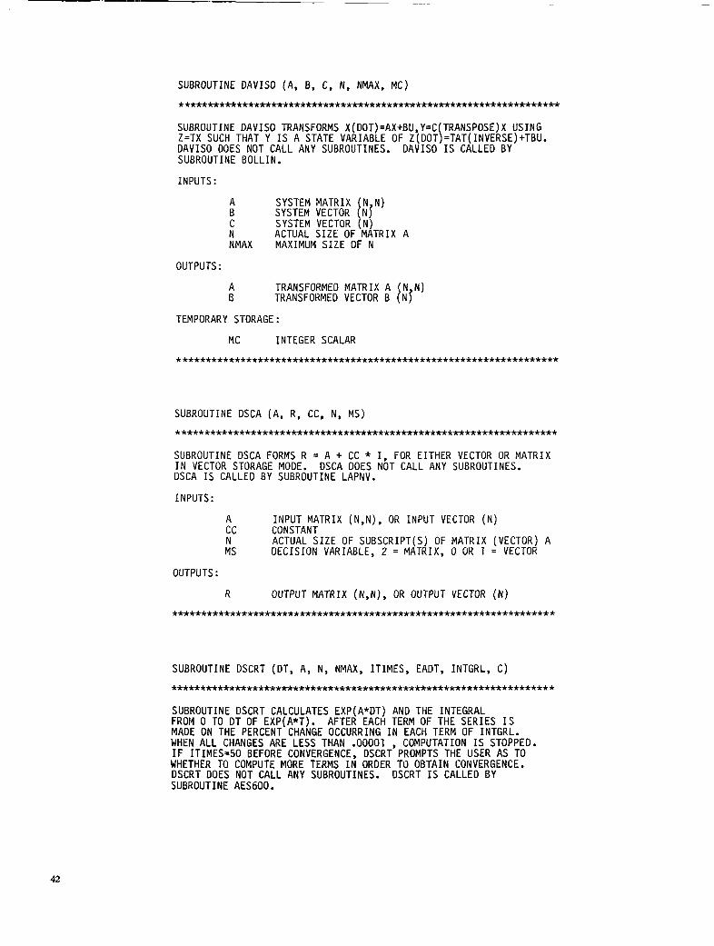
SUBROUTINE DAVISO (A, B, C, N, NMAX, MC)

. ................................................................. SUBROUTINE DAVISO TRANSFORMS X(DOT)=AX+BU,Y=C TRANSP0SE)X USING

DAVISO DOES NOT CALL ANY SUBROUTINES. DAVISO I S CALLED BY SUBROUTINE BOLLIN.

INPUTS:

Z=TX SUCH THAT y I s A STATE VARIABLE OF z(~oT~=TAT(INvERsE)+TBu.

A SYSTEM MATRIX N N)

C SYSTEM VECTOR (N) B SYSTEM VECTOR [ N j

N ACTUAL S I Z E OF MATRIX A NMAX MAXIMUM S I Z E OF N

OUTPUTS :

A TRANSFORMED MATRIX A N N) B TRANSFORMED VECTOR B [N j

TEMPORARY STORAGE:

MC INTEGER SCALAR

. . . . . . . . . . . . . . . . . . . . . . . . . . . . . . . . . . . . . . . . . . . . . . . . . . . . . . . . . . . . . . . . . .

SUBROUTINE DSCA (A, R, CC, N, MS)

. . . . . . . . . . . . . . . . . . . . . . . . . . . . . . . . . . . . . . . . . . . . . . . . . . . . . . . . . . . . . . . . . . SUBROUTINE DSCA FORMS R = A + CC * I, FOR EITHER VECTOR OR MATRIX I N VECTOR STORAGE MODE. DSCA DOES NOT CALL ANY SUBROUTINES. DSCA I S CALLED BY SUBROUTINE LAPNV.

INPUTS :

A INPUT MATRIX (N,N), OR INPUT VECTOR (N)

N ACTUAL S I Z E OF SUBSCRIPT(S) OF MATRIX (VECTOR) A cc CONSTANT

MS DECISION VARIABLE, 2 = MATRIX, 0 OR 1 = VECTOR

OUTPUTS :

R OUTPUT MATRIX (N,N) , OR OUTPUT VECTOR ( N ) . . . . . . . . . . . . . . . . . . . . . . . . . . . . . . . . . . . . . . . . . . . . . . . . . . . . . . . . . . . . . . . . . .

SUBROUTINE OSCRT (DT, A, N, NMAX, IT IMES, EADT, INTGRL, C)

. ................................................................. SUBROUTINE DSCRT CALCULATES EXP(A*DT) AND THE INTEGRAL FROM 0 TO DT OF EXP( A*T) . AFTER EACH TERM OF THE SERIES IS MADE ON THE PERCENT CHANGE OCCURRING I N EACH TERM OF INTGRL.

I F I T I M E S = 5 0 BEFORE CONVERGENCE, DSCRT’PROMPTS THE USER AS TO WHETHER TO COMPUTE MORE TERMS I N ORDER TO OBTAIN CONVERGENCE. DSCRT DOES NOT CALL ANY SUBROUTINES. DSCRT I S CALLED BY SUBROUTINE AES600.

WHEN A L L CHANGES ARE LESS THAN .00001 COMPUTATION I S STOPPED.

42

INPUTS :

D T T I M E STEP A INPUT MATRIX (N,N) N ACTUAL S I Z E OF MATRIX A NMAX MAXIMUM S I Z E OF N

OUTPUTS :

I T I M E S NO. OF TERMS I N SERIES EXPANSION EADT EXP(A*DT) (N,N) INTGRL INTEGRAL OF EXP(A*T) FROM T=O TO T=DT (N,N)

TEMPORARY STORAGE:

C VECTOR (N)

. . . . . . . . . . . . . . . . . . . . . . . . . . . . . . . . . . . . . . . . . . . . . . . . . . . . . . . . . . . . . . . . . .

SUBROUTINE EGCK (AAA, X, CPR, CPI , EX1, EX2, PLAM, N, NMAX)

. . . . . . . . . . . . . . . . . . . . . . . . . . . . . . . . . . . . . . . . . . . . . . . . . . . . . . . . . . . . . . . . . . SUBROUTINE EGCK PERFORMS THE EIGENVALUE AND EIGENVECTOR CHECK. I T FORMS (AAA * X) AND ( X * LAMBDA). EGCK DOES NOT CALL ANY SUBROUTINE. EGCK I S CALLED BY SUBROUTINE RICSS.

I NPUTS :

AAA ORIGINAL MATRIX FOR WHICH EIGENVALUES AND EIGENVECTORS WERE FOUND (N,N

X MODIFIED EIGENVECTOR MATRIX (N,N\ CPR VECTOR OF REAL EIGENVALUES (N) C P I VECTOR OF IMAGINARY EIGENVALUES ( N ) N ACTUAL S I Z E OF MATRIX AAA NMAX MAXIMUM S I Z E OF N

OUTPUTS :

EX1 AAA * X MATRIX (N,N) EX2 X * LAMBDA MATRIX (N,N)

TEMPORARY STORAGE:

PLAM MATRIX (N,N)

. . . . . . . . . . . . . . . . . . . . . . . . . . . . . . . . . . . . . . . . . . . . . . . . . . . . . . . . . . . . . . . . . .

SUBROUTINE EGVCTR ( M A , CPR, CPI, X, N2, TT, EXT, AR, AI , IPERN, 1 IPER, IOP2, NEMAX, ISEL, IHALF)

. ................................................................. SUBROUTINE EGVCTR OBTAINS THE N2 BY N2 MODIFIED EIGENVECTOR MATRIX X OF MATRIX AAA USING THE INVERSE ITERATION ALGORITHM. (THE EIGENVALUES OF AAA SHOULD HAVE BEEN PREVIOUSLY GENERATED USING SUBROUTINE EIGQR AND STORED I N CPR AND CPI. ) IEND SPECIFIES THE NUMBER OF PASSES THRU THE INVERSE ITERATION ALGORITHM. I F ISEL=D, ALL EIGENVECTORS ARE OBTAINED. I F ISEL IO, ONLY THE I S E L (AND NEXT ONE I F A COMPLEX P A I R ) I S

I F I S E L 0, THE ISELTH VECTOR I S PRINTED OUT AFTER EACH ITER. I F IHALF= l , THE F IRST N2 /2 VECTORS ARE OBTAINED. I F IHALF .NE. 1, A L L VECTORS ARE OBTAINED. EGVCTR CALLS SUBROUTINES ARRAY, FACTR, MATPRT, AND PRMUTE. EGVCTR I S CALLED BY SUBROUTINES AES400, AES800, AND RICSS.

OBTAINED.

43

INPUTS:

AAA

C PR

C P I

N 2 I OP2 NEMAX I S E L I H A L F

OUTPUTS :

X

MATRIX FOR WHICH EIGENVECTORS ARE TO BE OBTAINED

K k % ' O F REAL PARTS OF EIGENVALUES (N2)

VECTOR OF IMAGINARY PARTS OF EIGENVALUES (N2)

ACTUAL S I Z E OF MATRIX AAA P R I N T OPTION: 0, NO PRINT; 1, PRINT MAXIMUM S I Z E OF N 2 SELECTION OPTION SELECTION OPTION

(OF AAA)

(OF AAA)

MODIFIED EIGENVECTOR MATRIX OF AAA (N2,N2)

TEMPORARY STORAGE :

TT MATRIX N2 N2

AR VECTOR ( N 2 A I VECTOR ( N 2 1 IPERN INTEGER VECTOR (N2 1PER INTEGER VECTOR ( N 2 1

EXT MATRIX [Nz:NZJ

. . . . . . . . . . . . . . . . . . . . . . . . . . . . . . . . . . . . . . . . . . . . . . . . . . . . . . . . . . . . . . . . . .

SUBROUTINE EIGEN (A, EIGR, EIGI, EX1, S S S , S , I A , 16, LEX, MEX, 1 I B L , I C , EX4, N, NMAX)

. . . . . . . . . . . . . . . . . . . . . . . . . . . . . . . . . . . . . . . . . . . . . . . . . . . . . . . . . . . . . . . . . . SUBROUTINE EIGEN OBTAINS THE EIGENVALUES (EIGR AND E I G I ) OF N X N MATRIX A B Y F I R S T REDUCING ( I F A IS REDUCIBLE), THEN SCALING, HESSENBURG TRANSFORMING AND FINALLY APPLYING THE 'QR' ALGORITHM EIGEN CALLS SUBROUTINES SCALEA, CONDI, ARRAY, HSBG, AND EIGQR. EIGEN I S CALLED BY SUBROUTINES AES400 AND AES800.

INPUTS:

A N

MATRIX TO GET EIGENVALUES FOR (N,N) ACTUAL S I Z E OF MATRIX A

NMAX MAXIMUM S I Z E OF N

OUTPUTS :

EIGR VECTOR OF REAL PARTS OF EIGENVALUES (N) E I G I VECTOR OF IMAGINARY PARTS OF EIGENVALUES (N) S MATRIX A I N REDUCED AND SCALED FORM (N,N) LEX BLOCK-DIAGONALIZING PERMUTATION INTEGER

VECTOR (N) MEX INTEGER VECTOR OF S I Z E S OF EACH IRREDUCIBLE

BLOCK (N) MATRIX (N)

E X 4 VECTOR OF DIAGONAL ELEMENTS OF DIAGONAL SCALING

TEMPORARY STORAGE :

sss MATRIX [N:N{ EX1 MATRIX N N

I A INTEGER VECTOR ( N I B INTEGER VECTOR ( N I B L INTEGER VECTOR N I C INTEGER VECTOR I N 1

44

SUBROUTINE EIGQR (XR, N2, CR, CI, IOP, N2MAX)

. . . . . . . . . . . . . . . . . . . . . . . . . . . . . . . . . . . . . . . . . . . . . . . . . . . . . . . . . . . . . . . . . . SUBROUTINE EIGQR COMPUTES THE EIGENVALUES OF MATRIX XR USING THE QR ALGORITHM. THIS MATRIX MUST BE I N UPPER HESSENBERG FORM. THE MAXIMUM NUMBER OF QR ITERATIONS USED I N F I N D I N G ANY ONE EIGQR DOES NOT CALL ANY SUBROUTINES. EIGQR I S CALLED BY SUBROUTINES EIGEN, RICSS, AND ZEROES.

INPUTS :

XR M A T R I X ( I N UPPER HESSENBERG FORM) FOR WHICH EIGENVALUES ARE TO BE FOUND (N2,N2)

N 2 ACTUAL S I Z E OF MATRIX XR IOP PRINT OPTION

IOPIO, THE EIGENVALUES ARE WRITTEN ON U N I T 06 IOP=O, NO WRITING TAKES PLACE I O P 0, THE EIGENVALUES ARE WRITTEN ON U N I T 06 AND ON UNIT 02 (TERMINAL)

N2MAX MAXIMUM S I Z E OF N 2

OUTPUTS :

CR VECTOR OF REAL PARTS OF EIGENVALUES (N2) CI VECTOR OF IMAGINARY PARTS OF EIGENVALUES (N2)

. . . . . . . . . . . . . . . . . . . . . . . . . . . . . . . . . . . . . . . . . . . . . . . . . . . . . . . . . . . . . . . . . .

SUBROUTINE ESTMAT (AA, HH QQ, RRINV, KE PP, CR, CI, X, TS, XR, 1 TT, AAA, EXT, AR, A I , IPkR, IPERN, AOBLk, N, NM, N2, IOP1, IOP2, 2 NMAX, NMMAX, N2MAX)

. . . . . . . . . . . . . . . . . . . . . . . . . . . . . . . . . . . . . . . . . . . . . . . . . . . . . . . . . . . . . . . . . . SUBROUTINE ESTMAT SOLVES THE OPTIMAL LINEAR STATE ESTIMATION PROBLEM. I T SETS UP AN N2 BY N2 MATRIX AAA. USING MATRICES AA, HH, QQ, AND RRINV. ESTMAT OBTAINS THE KALMAN F I L T E R ERROR COVARIANCE, PP, AND THEN COMPUTES THE KALMAN F I L T E R GAINS, KE. ESTMAT CALLS SUBROUTINES MATPRT AND RICSS. ESTMAT I S CALLED BY SUBROUTINE AESBOO.

INPUTS:

AA HH QQ RRINV

I O P l I O P 2 N NM N 2 NMAX NMMAX N2MAX

OUTPUTS :

K E PP

SYSTEM MATRIX (N,N) MEASUREMENT MATRIX (NM,N) POWER SPECTRAL DENSITY MATRIX (N,N) (OF PLANT DISTURBANCE) ~ N V E R S E OF POWER S P E C ~ R A L DENSITY MATRIX (NM,NM) (OF MEASUREMENT NOISE) SCALING PRINT OPTION: 0, NO PRINT; 1, PRINT EIGENVECTOR PRINT OPTION: 0, NO PRINT; 1, P R I N T NUMBER OF STATE VARIABLES NUMBER OF MEASUREMENTS

MAXIMUM S I Z E OF N DIMENSION OF HAMILTONIAN MATRIX, 2 X N

MAXIMUM S I Z E OF NM MAXIMUM S I Z E OF N 2

KALMAN FILTER GAIN MATRIX (N,NM) KALMAN F I L T E R ERROR COVARIANCE MATRIX (N,N)

45

CR VECTOR OF REAL PARTS OF EIGENVALUES (N2) (OF AAA)

(OF AAA) C I VECTOR OF IMAGINARY PARTS OF EIGENVALUES (N2)

X MODIFIED EIGENVECTOR MATRIX OF AAA (N2,NZ) TS SCALING TRANSFORMATION VECTOR OF AAA ( N 2 ) AAA HAMILTONIAN MATRIX FOR KALMAN F I L T E R R I C C A T I

EQUATION (N2,N2)

TEMPORARY STORAGE :

XR T T EXT MATRIX (N2,NZ AR VECTOR (N2) A I VECTOR (N2) IPER INTEGER VECTOR ( N 2 ) IPERN INTEGER VECTOR ( N 2 ) ADBLE VECTOR (N X N)

. . . . . . . . . . . . . . . . . . . . . . . . . . . . . . . . . . . . . . . . . . . . . . . . . . . . . . . . . . . . . . . . . .

SUBROUTINE FACTR (A, PER, N, I A , I E R )

. . . . . . . . . . . . . . . . . . . . . . . . . . . . . . . . . . . . . . . . . . . . . . . . . . . . . . . . . . . . . . . . . . SUBROUTINE FACTR FORMS THE LOWER AND UPPER TRIANGULAR MATRICES OF INPUT MATRIX A, SUCH THAT UPPER * LOWER = A. FACTR DOES NOT CALL ANY SUBROUTINES. FACTR I S CALLED BY SUBROUTINE EGVCTR.

INPUTS :

A INPUT MATRIX (N,N) N ACTUAL S I Z E OF MATRIX A I A SAME AS N

OUTPUTS :

A INPUT MATRIX I N UPPER AND LOWER TRIANGULAR ~~

PER TRANSPOSITION VECTOR FOR MATRIX A ( N ) I ER ERROR OPTION.

FORM (N,N) ~

I F I E R .NE. 0, FACTR IS WRONG I F I E R .EQ. 0, FACTR HAS WORKED CORRECTLY

. . . . . . . . . . . . . . . . . . . . . . . . . . . . . . . . . . . . . . . . . . . . . . . . . . . . . . . . . . . . . . . . . .

SUBROUTINE FRPOLY ( Z l , 22, DD, HZ, 6, AMP, PHA, N )

. . . . . . . . . . . . . . . . . . . . . . . . . . . . . . . . . . . . . . . . . . . . . . . . . . . . . . . . . . . . . . . . . . SUBROUTINE FRPOLY EVALUATES TRANSFER FUNCTION Z2(S) / Z l ( S ) FOR S = 6.28 * HZ * J. FRPOLY DOES NOT CALL ANY SUBROUTINES. FRPOLY IS CALLED BY SUBROUTINE FRQP.

INPUTS:

z1 DENOMINATOR COEFFICIENT VECTOR 22 NUMERATOR COEFFICIENT VECTOR DD DOUT OR 0.0 HZ FREQUENCY N S I Z E OF COEFFICIENT VECTORS

OUTPUTS :

G COMPLEX TRANSFER FUNCTION

AMP PHA PHASE

AMPLITUDE

******+***********************************************************

1 ISPACE, TSFTR) SUBROUTINE FRQP ( Z l , 2 2 , DD, N, F I , DELF, IF, FREQ, AMP, PHASE,

. . . . . . . . . . . . . . . . . . . . . . . . . . . . . . . . . . . . . . . . . . . . . . . . . . . . . . . . . . . . . . . . . . SUBROUTINE FRQP GENERATES FREQUENCY RESPONSE AMP. AND PHASE, GIVEN TRANSFER FUNCTION NUMERATOR AND DENOMINATOR POLYNOMIAL COEFFICIENTS (GENERATED BY SUBROUTINE BOLLIN). FRQP CALLS SUBROUTINE FRPOLY, WHICH COMPUTES AMPLITUDE AND PHASE. FRQP IS CALLED BY SUBROUTINE FRSPNS.

INPUTS :

z1 22 DD N TSFTR F I DELF I F I SPACE

OUTPUTS :

FREQ AMP PHASE

DENOMINATOR POLYNOMIAL COEFFICIENT VECTOR NUMERATOR POLYNOMIAL COEFFICIENT VECTOR DOUT OR 0.0 S I Z E OF COEFFICIENT VECTORS T IME SCALE FACTOR I N I T I A L FREQUENCY SPACING BETWEEN FREQUENCY POINTS NUMBER OF DESIRED POINTS TO BE GENERATED CONTROLS FREQUENCY OF PRINTOUT FOR FREQ, AMP AND PHASE

FREQUENCY VECTOR AMPLITUDE VECTOR PHASE VECTOR

. . . . . . . . . . . . . . . . . . . . . . . . . . . . . . . . . . . . . . . . . . . . . . . . . . . . . . . . . . . . . . . . . .

SUBROUTINE FRSPNS ( A B, C DD, IOUT, J I N N TSFTR DXM1, DXV l , 1 DXVZ, DXV3, EXM1, EkV1, EkV2, NMAX, NOMAk bDCOF, bNCOF, FI , 2 DELF, IF, FREQ, AMP, PHASE, ISPACE, IPRNT~

. . . . . . . . . . . . . . . . . . . . . . . . . . . . . . . . . . . . . . . . . . . . . . . . . . . . . . . . . . . . . . . . . . SUBROUTINE FRSPNS COMPUTES THE FREQUENCY RESPONSE OF THE I O U T OUTPUT TO THE J I N I N P U T OF THE SYSTEM XDOT = A*X + B*U - Y = C*X

SUBROUTINE AES500.

INPUTS:

FRSPNS CALLS SUBROUTINES BOLLIN AND FRQP. FRSPNS IS C A L ~ E D BY

A B C DD I OUT J I N N TSFTR N MAX NOMAX F I DELF I F ISPACE

IPRNT

SYSTEM MATRIX [N,NC) SYSTEM MATRIX N,N)

SYSTEM MATRIX (N0,N) DOUT OR 0.0 INDEX OF OUTPUT INDEX OF I N P U T ACTUAL SIZE OF MATRIX A TIME SCALE FACTOR MAXIMUM S I Z E O F N MAXIMUM S I Z E OF NO I N I T I A L FREQUENCY SPACING BETWEEN FREQUENCY POINTS NUMBER OF DESIRED POINTS TO BE GENERATED CONTROLS FREQUENCY OF PRINTOUT FOR FREQ, AMP AND PHASE PRINT OPTION, 0 I F STANDARD, 1 I F EXTENDED

41

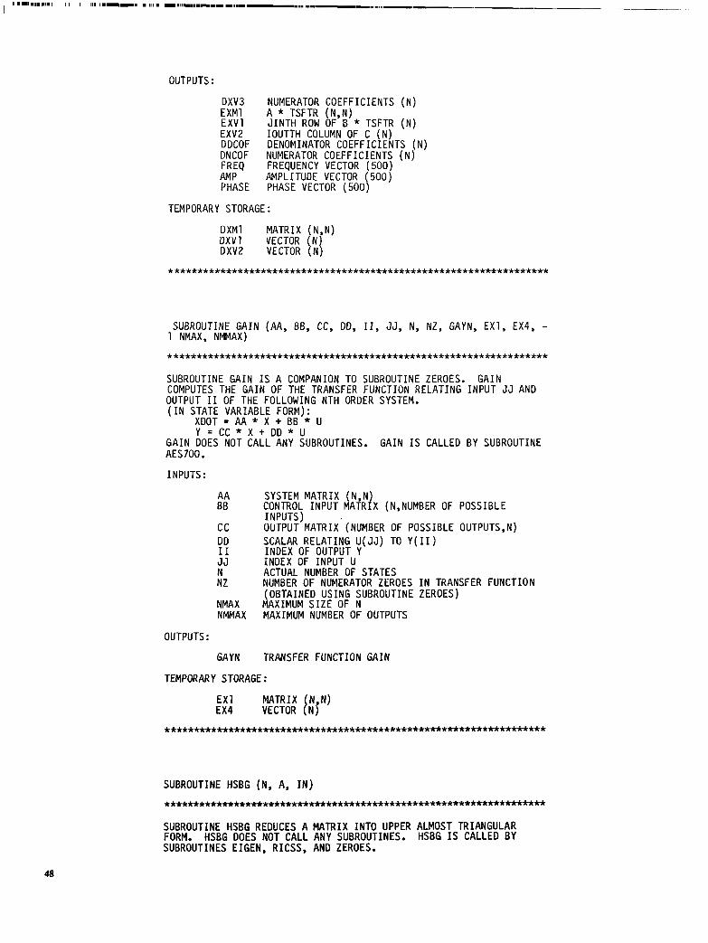
OUTPUTS :

DXV3 NUMERATOR COEFFICIENTS (N) EXMl A * TSFTR (N.N) E X V l J I N T H ROW OF-B ' * TSFTR (N) EXV2 IOUTTH COLUMN OF C (N) DDCOF DENOMINATOR COEFFICIENTS (N) DNCOF NUMERATOR COEFFICIENTS (N) . FREO FREOUENCY VECTOR (500) AMP . AMPLITUDE VECTOR '500 j PHASE PHASE VECTOR (500\

TEMPORARY STORAGE :

DXMl MATRIX (N,N)

. .................................................................

1 NMAX, NMMAX) SUBROUTINE GAIN (AA, BB, CC, DO, 11, JJ, N, NZ, GAYN, EX7, EX4, -

. . . . . . . . . . . . . . . . . . . . . . . . . . . . . . . . . . . . . . . . . . . . . . . . . . . . . . . . . . . . . . . . . . SUBROUTINE GAIN I S A COMPANION TO SUBROUTINE ZEROES. GAIN COMPUTES THE GAIN OF THE TRANSFER FUNCTION RELATING INPUT JJ AND OUTPUT I 1 OF THE FOLLOWING NTH ORDER SYSTEM.

I N STATE VARIABLE FORM): XDOT = AA *-X + ~ B B ' * U Y = C C * X + D D * U

G A I N DOES NOT CALL ANY SUBROUTINES. GAIN I S CALLED BY SUBROUTINE AES700.

INPUTS:

AA BB

c c DD I 1 JJ N NZ

NMAX NMMAX

OUTPUTS :

GAYN

SYSTEM MATRIX (N,N) CONTROL INPUT MATRIX (N,NUMBER OF POSSIBLE INPUTS) OUTPUT'MATRIX (NUMBER OF POSSIBLE OUTPUTS,N) SCALAR RELATING U(JJ) TO Y(II I

. .

INDEX OF OUTPUT Y INDEX OF INPUT U ACTUAL NUMBER OF STATES NUMBER OF NUMERATOR ZEROES (OBTAINED USING SUBROUTINE MAXIMUM S I Z E OF N MAXIMUM NUMBER OF OUTPUTS

TRANSFER FUNCTION GAIN

I N TRANSFER FUNCTION ZEROES)

TEMPORARY STORAGE :

EX4 VECTOR [ N j EX1 MATRIX N N)

..................................................................

SUBROUTINE HSBG (N, A, I N )

................................................................. SUBROUTINE HSBG REDUCES A MATRIX INTO UPPER ALMOST TRIANGULAR FORM. HSBG DOES NOT CALL ANY SUBROUTINES. HSBG I S CALLED BY SUBROUTINES EIGEN, RICSS, AND ZEROES.

I

INPUTS :

N ACTUAL S I Z E OF MATRIX A A INPUT MATRIX (N,N) I N MAXIMUM S I Z E OF MATRIX A I N THE CALLING PROGRAM;

I N = N, WHEN MATRIX A I S I N VECTOR STORAGE MODE.

OUTPUTS :

A OUTPUT MATRIX (N,N)

. ................................................................. SUBROUTINE ICRSP (EX1, C, ICMTX, AMPIN, DT, TIME, TYOUT, XNEW,

2 NAME, IONPLT) 1 XOLD, T T I T , TTOP, TYTIT, IEXT, N, NOUT, NMAX, NOUTMX, ITRMX, I P ,

. . ................................................................ SUBROUTINE ICRSP COMPUTES MULTIPLE IN IT IAL CONDITION RESPONSES OF THE SYSTEM: XDOT=A*X AND TYOUT=C*X BY SOLVING THE DIFFERENCE EQUATION: XNEW=EXl*XOLD T H I S SUBROUTINE REQUIRES THAT THE STATE TRANSITION MATRIX, EXP(A*DT), BE SUPPLIED AS INPUT MATRIX "EX1". DESIRED I N I T I A L CONDITION MAGNITUDES ARE SUPPLIED AS VECTOR 'AMPIN' AND THE

SELECTED BY APPROPRIATELY DEFINING ELEMENTS OF THE MATRIX ' ICMTX'. ICRSP CALLS PLOTTING SUBROUTINES ONLY. ICRSP I S CALLED BY SUBROUTINE AES600.

INPUTS:

DESIRED I N I T I A L CONDITION-OUTPUT RESPONSE COMBINATIONS ARE

C EX1 STATE TRANSITION, EXP(A*DT), MATRIX (N,N)

SYSTEM OUTPUT MATRIX (NOUT,N) ICMTX MATRIX OF ZEROES AND ONES (N,NOUT).

ONES ARE PLACED I N SELECTED MATRIX POSITIONS TO INDICATE THE I N I T I A L CONDITION RESPONSES DESIRED. THE FIRST INDEX I S 'STATE', AND THE SECOND I S 'OUTPUT'. THUS SUBROUTINE ICRSP MAY CALCULATE AS MANY AS N*NOUT I N I T I A L CONDITION RESPONSES.

AMPIN VECTOR OF INPUT INITIAL CONDITION AMPLITUDES (N) DT T IME STEP T T I T PLOT T I T L E ( 1 2 ) TTOP PLOT T I T L E (12) T Y T I T Y A X I S T I T L E ( 4 ) N ACTUAL S I Z E OF STATE TRANSITION MATRIX NOUT ACTUAL NUMBER OF POSSIBLE OUTPUTS

NOUTMX MAXIMUM S I Z E OF NOUT NMAX MAXIMUM S I Z E OF N

ITRMX NUMBER OF DESIRED TIME RESPONSE POINTS

INCREASES BY ONE FOR EACH FRAME

(PARTITIONED DATASET THAT HOLDS PLOT ENTITIES)

1, I F ONLINE PLOTS

I P PLOT ENTITY INDEX (USED BY PLOTSUBS ONLY)

NAME NAME OF PLOT DATASET ( 9 ) (USED BY PLOTSUBS ONLY)

IONPLT 0, I F OFFLINE PLQTS

OUTPUTS :

T I M E VECTOR OF TIME POINTS ( ITRMX) (SINGLE PRECISION)

TYOUT MATRIX OF OUTPUT TRANSIENT RESPONSES FOR ANY ONE S P E C I F I C I N I T I A L CONTIDION. (ITRMX,NOUT) (SINGLE PRECISION)

I P PLOT ENTITY INDEX' (USED BY PLOTSUBS ONLY) INCREASES BY ONE FOR EACH FRAME

TEMPORARY STORAGE:

XNEW VECTOR ( N XOLD VECTOR ( N ] I E X T INTEGER VECTOR (N)

.................................................................. 49

, ,. . ..

SUBROUTINE LAPNV (A, X, 6, QIN, NIN, WORK)

. ................................................................. SUBROUTINE LAPNV SOLVES THE LYAPUNOV EQUATION, X*A' + A*X+B=O WHERE A ' I S A-TRANSPOSE, A, B, AND X ARE A L L NXN MATRICES I N VECTOR STORAGE MODE, B IS SYMMETRIC ON INPUT, AND X I S SYMMETRIC ON OUTPUT. STEP 1 CALCULATE X(0) = A'*B*A STEP 2 THE EXACT SOLUTION X I S THE L I M I T OF THE SEQUENCE X(M)

COMPUTE EACH TERM X(M+l) RECURSIVELY, BASED ON X(M) AS FOLLOWS, X(M+11= X(MI + U(MI*XIM) * U ' I M )

WHERE THE M REFERS TO THE M-TH TERM OF THE SEQUENCE.

LAPNV CALL^ SU~ROU~INES DSCA, MXINV, MXMLT, MXTRA, AND MXADD. LAPNV I S CALLED BY SUBROUTINES COVAR AND LYPCK.

INPUTS:

A LYAPUNOV EQUATION MATRIX (NIN,NIN B LYAPUNOV EQUATION MATRIX (NIN,NIN)) Q I N CONVERGENCE FACTOR (TYPICALLY . 1 ) N I N ACTUAL S I Z E OF MATRIX A WORK( 1) CONVERGENCE CHECK CRITERION (TYPICALLY 1 .E-6)

OUTPUTS :

X OUTPUT MATRIX (NIN,NIN)

TEMPORARY STORAGE:

WORK VECTOR ( 2 X N I N X N I N )

. .................................................................

SUBROUTINE LOGSET (TMIN, TMAX, TNARR, I N T )

. ................................................................. SUBROUTINE LOGSET CALCULATES THE DECADES NECESSARY TO INCLUDE THE MINIMUM AND MAXIMUM OF THE DATA TO BE PLOTTED. LOGSET DOES NOT CALL ANY SUBROUTINES.

INPUTS:

TNARR ACTUAL DATA MINIMUM AND MAXIMUM (2) LOCATION 1 HOLDS THE MINIMUM LOCATION 2 HOLDS THE MAXIMUM

OUTPUTS :

TMIN MINIMUM DECADE FOR PLOTTING TMAX MAXIMUM DECADE FOR PLOTTING I N T NUMBER OF INTERVALS FOR LOG A X I S

..................................................................

50

SUBROUTINE LYPCK (A, Q, XHT, E, R, EXI , WORK, N, NMAX)

SUBROUTINE LYPCK COMPUTES THE RESIDUAL AND ERROR MATRICES ASSOCIATED WITH THE LYAPUNOV EQ.

A*X + X*A**T + 0 = 0 WHERE

SOLUTION--XHT RESIDUAL--R=A*XHT + XHT*A**T + Q ERROR-----E=XHT - X

WHERE A*E + E*A**T - R = 0

WORK VECTOR 'WORK' MUST BE DIMENSIONED 1=2*N**2 BEFORE COMPUTING E, R~ IS SYMMETRIZED. '

ERROR INDEX, TR(E)/TR(XHT), AND THE NORMALIZED DIAGONAL ELEMENTS THE TRACES OF XHT R, & E ARE PRINTED OUT; ALSO THE NORMALIZED

OF THE ERROR MATRIX ARE PRINTED OUT. LYPCK CALLS SUBROUTINES MATPRT, ARRAY, AND LAPNV. LYPCK I S CALLED BY SUBROUTINE AES800.

INPUTS :

A LYAPUNOV EQUATION MATRIX Q LYAPUNOV EQUATION MATRIX XHT LYAPUNOV SOLUTION MATRIX (N,N N ACTUAL S I Z E OF MATRIX A NMAX MAXIMUM S I Z E OF N

OUTPUTS :

E R

ERROR MATRIX (N,N) RESIDUAL MATRIX (N,N)

TEMPORARY STORAGE:

EX1 MATRIX (N,N) WORK VECTOR ( 2 X N X N )

. ...................................................................

SUBROUTINE MATCHG

.................................................................... SUBROUTINE MATCHG I S USED FOR CHANGING MATRICES AND DIMENSIONS USING NAMELIST 'MATDAT'. THE CHANGES I N MATDAT ARE READ I N FROM THE TERMINAL. DATA I S TRANSFERRED TO PROGRAM AESOP V I A COMMONS 'ABETC' AND 'DIMS'. MATCHG DOES N O T CALL ANY SUBROUTINES. ' MATCHG I S CALLED BY SUBROUTINE AES200.

SUBROUTINE MATIN

**~*************m**~***1Hr***1Hr1Hr*m***m**m**m********

SUBROUTINE MATIN I S USED FOR INPUTTING MATRICES AND DIMENSIONS FOR A 'SMALL' LQR/KALMAN FILTER PROBLEM TESTCASE. I T ALSO PRINTS OUT THE REFS NAMELIST. DATA I S PROVIDED FOR A 3RD ORDER TEST CASE HAVING TWO CONTROLS AND TWO SET-POINT OUTPUTS, TWO DISTURBANCES AND ONE NOISY MEASUREMENT. MATIN CALLS SUBROUTINE MATPRT. MATIN I S CALLED BY SUBROUTINE AESPOO.

m*****m***m*.**m1Hr"- ******* . . . .

51

SUBROUTINE MATPRT (A, N, M, NMAX)

*********************************w+*********~**********************

SUBROUTINE MATPRT PRINTS MATRIX A TEN COLUMNS PER PAGE. THE DEVICE ON WHICH THE PRINTING TAKES PLACE I S CONTROLLED B Y ' I U N I T ' .

MATPRT DOES NOT CALL ANY SUBROUTINES. MATPRT I S CALLED BY SUBROUTINES AESPOO, AES300, AES400, AES600, AES700, AES800, COVAR, CTBL, EGCK, LYPCK, MATIN, MATRD, MODSHP, OBSBL, RESI, RICCHK, RICSS, AND UNRML.

INPUTS:

IUNIT=2---TERMINAL, IUNIT=6---LINEPRINTER.

A MATRIX TO BE PRINTED (N,M) N NUMBER OF ROWS I N MATRIX A M NUMBER OF COLUMNS I N MATRIX A NMAX MAXIMUM S I Z E OF N

******************************************************************

SUBROUTINE MATRD

SUBROUTINE MATRD I S USED FOR INPUTTING MATRICES, DIMENSIONS, AND REFS USING NAMELISTS 'MATDAT' AND 'REFS'. MATDAT AND REFS ARE READ I N FROM U N I T 33. DATA I S TRANSFERRED TO PROGRAM AESOP V I A COMMONS 'COMl', 'ABETC', 'DIMS', 'DIMS2', AND 'REFCOM'. MATRD CALLS SUBROUTINE MATPRT. MATRD I S CALLED BY SUBROUTINE AESZOO.

SUBROUTINE MODSHP (A, B, CI , N, NMAX)

. . . . . . . . . . . . . . . . . . . . . . . . . . . . . . . . . . . . . . . . . . . . . . . . . . . . . . . . . . . . . . . . . SUBROUTINE MODSHP CALCULATES MODE SHAPES I N MAGNITUDE AND ANGLE (DEGREE) FORM. MODSHP CALLS SUBROUTINE MATPRT. MODSHP I S CALLED BY SUBROUTINES AES400, AES800, AND RICSS.

INPUTS:

A MODIFIED EIGENVECTOR MATRIX (N,N

N ACTUAL NUMBER OF EIGENVALUES NMAX MAXIMUM S I Z E OF N

C I VECTOR OF IMAGINARY EIGENVALUES I N )

OUTPUTS :

B MODESHAPE I N MAGNITUDE AND ANGLE FORM (N,N)

. . . . . . . . . . . . . . . . . . . . . . . . . . . . . . . . . . . . . . . . . . . . . . . . . . . . . . . . . . . . . . .

52

SUBROUTINE MXADD (A, B, R, N, M)

SUBROUTINE MXADD ADDS TWO IDENTICALLY SIZED MATRICES TO FORM A RESULTANT MATRIX. R CAN BE THE SAME AS A OR B I N THE CALLING PROGRAM. MXADD DOES NOT CALL ANY SUBROUTINES. MXADD I S CALLED BY SUBROUTINE LAPNV.

INPUTS:

A F IRST INPUT MATRIX (N,M)

M NUMBER OF COLUMNS I N MATRICES A, B, AND R

B N

SECOND INPUT MATRIX (N,M) NUMBER OF ROWS I N MATRICES A, B, AND R

OUTPUTS :

R OUTPUT MATRIX (N,M)

. .................................................................

SUBROUTINE MXINV (A, N, D, L, M)

. . . . . . . . . . . . . . . . . . . . . . . . . . . . . . . . . . . . . . . . . . . . . . . . . . . . . . . . . . . . . . . . . . SUBROUTINE MXINV INVERTS A DOUBLE PRECISION MATRIX I N VECTOR

CALCULATED BUT I S ZERO I F THE MATRIX BEING INVERTED I S SINGULAR. MXINV DOES NOT CALL ANY SUBROUTINES. MXINV I S CALLED BY SUBROUTINES AES300, AES800, CTBL, LAPNV, AND RICSS.

INPUTS :

STORAGE MODE BY USING THE GAUSS-JORDAN METHOD. THE DETERMINANT I S

A N

MATRIX TO BE INVERTED, VECTOR STORAGE MODE (N,N) ACTUAL S I Z E OF MATRIX A

OUTPUTS :

A MATRIX INVERTED FORM, VECTOR STORAGE MODE (N,N) D SCALAR DETERMINANT (ZERO I F MATRIX A I S SINGULAR)

TEMPORARY STORAGE :

L INTEGER VECTOR ( N M INTEGER VECTOR ( N I

. .................................................................

SUBROUTINE MXMLT (A, B, R, N, L, M)

. ................................................................. SUBROUTINE MXMLT MULTIPL IES TWO MATRICES I N VECTOR STOGAGE MODE TO FORM A RESULTANT MATRIX I N VECTOR STORAGE MODE. MXMLT DOES NOT CALL ANY SUBROUTINES. MXMLT I S CALLED BY SUBROUTINE LAPNV.

INPUTS :

L NUMBER OF COLUMNS IN MATRIX A AND ROWS I N MATRIX B

M NUMBER OF COLUMNS I N MATRIX B

OUTPUTS :

R OUTPUT MATRIX (N,M)

****m*K**.*****lt*m+*****mH******ti*********

53

SUBROUTINE MXTRA (A, R, N, M)

. ................................................................ SUBROUTINE MXTRA TRANSPOSES AN N BY M MATRIX A I N VECTOR STORAGE MOUE TO FORM AN M BY N MATRIX R I N VECTOR STORAGE MODE. MXTRA DOES NOT CALL ANY SUBROUTINES. MXTRA I S CALLED BY SUBROUTINE LAPNV.

INPUTS:

A MATRIX TO BE TRANSPOSED (N,M) N NUMBERS OF ROWS I N MATRIX A

AND COLUMNS I N MATRIX R M NUMBERS OF COLUMNS I N MATRIX A

AND ROWS I N MATRIX R

OUTPUTS :

R RESULTANT MATRIX (M,N)

SUBROUTINE NRML (A, B, C, H, Q, RINV, D, DOUT, CSP, N, NC, NO, NM, 1 ND, NMAX, NCMAX, NOMAX, NMMAX, F L 3 4 )

. ................................................................. SUBROUTINE NRML READS FOUR NORMALIZATION VECTORS FROM NAMELIST NRMS AND NORMALIZES THE A, B, C, H, Q, RINV, D, DOUT, AND CSP MATRICES. THE SYSTEM THUS REPRESENTED IS DEFINED BY NORMALIZED STATE, CONTROL, OUTPUT, MEASUREMENT, AND SET POINT VECTORS. THE NORMALIZATION VECTORS ARE TRANSFERRED TO THE MAIN PROGRAM THROUGH COMMON 'NORMS'. NRML DOES NOT CALL ANY SUBROUTINES. NRML I S CALLED BY SUBROUTINE AES400.

INPUTS:

A B C H Q

RINV

D DOUT

CSP N NC NO NM ND NMAX NCMAX NOMAX NMMAX FL34

UN-NORMALIZED SYSTEM MATRIX (N,N) UN-NORMALIZED CONTROL INPUT MATRIX (N,NC) UN-NORMALIZED OUTPUT MATRIX (N0,N

UN-NORMALIZED POWER SPECTRAL DENSITY MATRIX OF

UN-NORMALIZED INVERSE OF POWER SPECTRAL DENSITY

UN-NORMALIZED MEASUREMENT MATRIX /NM,N)

PLANT DISTURBANCE (N,N)

MATRIX OF MEASUREMENT NOISE (NM,NM) UN-NORMALIZED DISTURBANCE INPUT MATRIX (N.ND) UN-NORMALIZED FEED FORWARD MATRIX FOR NON-ZERO SET POINT REGULATOR (N0,NC) UN-NORMALIZED SET POINT OUTPUT MATRIX (NC,N)

. - .

ACTUAL NUMBER OF STATES ACTUAL NUMBER OF CONTROL INPUTS ACTUAL NUMBER OF OUTPUTS ACTUAL NUMBER OF MEASUREMENTS ACTUAL NUMBER OF DISTURBANCE INPUTS MAXIMUM S I Z E OF N MAXIMUM S I Z E OF NC MAXIMUM S I Z E O F NO MAXIMUM S I Z E OF NM LOGICAL VARIABLE, ON INPUT

L . E , NORMALIZATION VECTOR INFORMATION (NAMELIST NRMS) NEEDS TO BE READ IN

TRUE, NORMALIZATION VECTOR INFORMATION NAMELIST NRMS HAS ALREADY BEEN READ I N

54

I

OUTPUTS :

A B C H Q R INV

D

DOUT

CSP F L 3 4

NORMALIZED SYSTEM MATRIX (N,N) NORMALIZED CONTROL INPUT MATRIX (N,NC) NORMALIZED OUTPUT MATRIX (N0.N

NORMALIZED POWER SPECTRAL DENSITY MATRIX 0 PLANT DISTURBANCE (N,N)

MATRIX OF MEASUREMENT NOISE (NM,NM) NORMALIZED INVERSE OF POWER SPECTRAL DENS1

NORMALIZED DISTURBANCE INPUT MATRIX (N,ND)

NORMALIZED MEASUREMENT MATRIX 2NM.N)

NORMALIZED FEED FORWARD MATRIX FOR

NORMALIZED SET POINT OUTPUT MATRIX NC,N) NON-ZERO SET POINT REGULATOR (NO,NC 1 LOGICAL VARIABLE, ON OUTPUT SET TO TRUE I F NAMELIST NRMS HAS BEEN READ I N

. "

IF

TY

..................................................................

SUBROUTINE OBSBL (H, T, CI , HT, EX1, N, NR, NRMAX, NMAX)

. ................................................................. SUBROUTINE OBSBL COMPUTES THE OBSERVABILITY MATRIX HT FOR THE

NOTE: FOR A COMPLEX EIGENVALUE PAIR. THE CORRESPONDING TWO COLUMN LINEAR SYSTEM DESCRIBED BY XDOT=A*X + B*U, AND Y=H*X.

ELEMENTS I N HT ARE STORED AS MAGNITUDE AND ANGLE ( I N DEGREES) RESPECTIVELY. OBSBL CALLS SUBROUTINE MATPRT. OBSBL I S CALLED BY SUBROUTINE AES400.

INPUTS:

H SYSTEM OUTPUT MATRIX (NR,N) T MODIFIED EIGENVECTOR MATRIX OF MATRIX A (N,N) C I VECTOR OF IMAG PARTS OF THE EIGENVALUES (N)

N ACTUAL NUMBER OF COLUMNS I N MATRIX H (OF MATRIX A)

NR ACTUAL NUMBER OF ROWS I N MATRIX H NRMAX MAXIMUM S I Z E OF NR NMkX MAXIMUM S I Z E OF N

OUTPUTS:

HT OBSERVABILITY MATRIX (NR,N

EX1 OBSERVABILITY MATRIX (NR,N) ( I N MAGNITUDE AND PHASE AN 6 LE FORM)

........................................................................

SUBROUTINE ORDER (CR, CI , NE, EPS)

...................................

GIVEN A SET OF NE EIGENVALUES, SYMMETRICALLY LOCATED WITH RESPECT TO THE IMAGINARY AXIS. SUBROUTINE ORDER PLACES ONES WITH POSITIVE REAL PARTS I N F I R S T N E / 2 LOCATIONS. CORRESPONDING SYMMETRIC EIGENVALUES WITH NEGATIVE REAL PARTS ARE PUT I N LOCATIONS NE/2 + 1 THROUGH NE. EPS I S THE CONVERGENCE CRITERION USED I N DETERMINING I F A P A I R OF EIGENVALUES ARE SYMMETRIC. ORDER DOES NOT CALL ANY SUBROUTINES. ORDER I S CALLED BY SUBROUTINE RICSS.

55

I

INPUTS:

CR VECTOR OF REAL PARTS OF EIGENVALUES UNORDERED (NE)

CI VECTOR OF IMAGINARY PARTS OF EIGENVALUES UNORDERED (NE)

NE NUMBER OF EIGENVALUES EPS CRITERION FOR SYMMETRY

OUTPUTS :

CR VECTOR OF REAL PARTS OF EIGENVALUES ORDERED (NE)

ORDERED (NE) CI VECTOR OF IMAGINARY PARTS OF EIGENVALUES

..................................................................

SUBROUTINE POLMPY (X, Y, Z, NX, NY, NZ)

. ................................................................. SUBROUTINE POLMPY MULTIPLIES X*Y=Z (THE LEADING POLYNOMIAL COEFFICIENT I S ASSUMED TO BE UNITY). POLMPY DOES NOT CALL ANY ANY SUBROUTINES. POLMPY I S CALLED BY SUBROUTINE DANSKY.

INPUTS:

X POLYNOMIAL COEFFIENT VECTOR (NX) Y POLYNOMIAL COEFFIENT VECTOR (NY) NX ORDER OF POLYNOMIAL FOR WHICH VECTOR X I S THE

NY ORDER OF POLYNOMIAL FOR WHICH VECTOR Y I S THE L I S T OF COEFFICIENTS (OTHER THAN THE F I R S T )

L I S T OF COEFFICIENTS (OTHER THAN THE F I R S T )

OUTPUTS :

Z X VECTOR * Y VECTOR (NZ) NZ ORDER OF POLYNOMIAL FOR WHICH VECTOR Z I S THE


Z X VECTOR * Y VECTOR (NZ) NZ ORDER OF POLYNOMIAL FOR WHICH VECTOR Z I S THE


..................................................................

SUBROUTINE PREREQ (WHEN, ICA, IAND, MZ, 11)

.................................................................. SUBROUTINE PREREQ CHECKS TO SEE I F PREREQUISITE CASES HAVE BEEN DONE FOR THE CASE ABOUT TO BE RUN. I F NOT, IT PRINTS OUT WHAT THE PREREQUISITES ARE. PREREQ DOES NOT CALL ANY SUBROUTINES. PREREQ I S CALLEO BY SUBROUTINES AES100, AESPOO, AES300, AES400, AESSOO, AES600, AES700, AND AES800.

INPUTS:

WHEN LOGICAL MATRIX OF PREREQS (450,50) I C A VECTOR OF CASE NUMBERS TO BE DONE (1000) MZ WHICH CASE I S TO BE CHECKED FOR PREREOUISITES I1 WHICH ROW OF MATRIX 'WHEN' IS TO BE LOOKED AT

OUTPUTS :

IAND DECISION VARIABLE, 0 IF PREREQUISITES HAVE BEEN DONE, 1 I F PREREQUISITES HAVE NOT BEEN DONE

....................................................................

56

I

SUBROUTINE PRMUTE (X, ITRANS, IA, NE, LA, NEMAX)

. ................................................................ SUBROUTINE PRMUTE PERMUTES ELEMENTS I N L A COLUMN OF NE BY N E MATRIX X AS DICTATED BY TRANSPOSITION VECTOR ITRANS. ITRANS I S PRODUCED, I N T H I S CASE, BY SUBROUTINE FACTR. PRMUTE DOES NOT CALL ANY SUBROUTINES. PRMUTE I S CALLED BY SUBROUTINE EGVCTR.

I NPUTS :

X MATRIX TO BE PERMUTED (NE,NE) ITRANS TRANSPOSITION VECTOR (NE) NE L A

ACTUAL S I Z E OF MATRIX X SPECIFIC COLUMN OF MATRIX X TO BE PERMUTED BY THE TRANSPOSITION VECTOR ITRANS

NEMAX MAXIMUM S I Z E OF NE

OUTPUTS :

X INPUT MATRIX I N PERMUTED FORM (NE,NE)

TEMPORARY STORAGE:

I A INTEGER VECTOR (NE)

. .................................................................

1 NMAX) SUBROUTINE REDU (VARO, SS, S, IN, JBL, INBL, IOR, NBL, I B L , I C , N,

. . ................................................................ SUBROUTINE REDU USES HARARYS METHOD FOR REDUCTION OF A REDUCIBLE

REDU I S CALLED BY SUBROUTINE CONDI. MATRIX TO BLOCK DIAGONAL FORM. REDU DOES NOT CALL ANY SUBROUTINE.

INPUTS:

VARO MATRIX TO BE REDUCED (N,N) N ACTUAL S I Z E OF MATRIX VARO NMAX MAXIMUM S I Z E OF N

OUTPUTS :

S BLOCK DIAGONAL MATRIX ( N, N) I N B L NUMBER OF REDUCIBLE BLOCKS IOR BLOCK-DIAGONALIZING PERMUTATION INTEGER

VECTOR (N)

BLOCK (N) NBL INTEGER VECTOR OF S I Z E S OF EACH IRREDUCIBLE

TEMPORARY STORAGE :

ss MATRIX (N,N) I N INTEGER VECTOR N J B L INTEGER VECTOR I N / I B L INTEGER VECTOR N I C INTEGER VECTOR (N)

. .................................................................

57

SUBROUTINE R E S I (C, B, EIGR, E I G I , R, EXA, N, NC, NO, NMAX, NOMAX)

................................................................. SUBROUTINE R E S I COMPUTES THE RESIDUE MATRICES FOR THE LINEAR SYSTEM, XDOT=A*X + B*U, AND, Y=C*X WHERE THE SYSTEM I S ASSUMED TO BE I N BLOCK-DIAGONAL FORM. MATRICES C AND B ARE INPUT TO THE PROGRAM. MATRIX C I S ASSUMED TO HAVE BEEN TRANSFORMED TO THE FORM CORRESPONDING TO BLOCK-DIAGONAL A MATRIX USING SUBROUTINE OBSBL. MATRIX B IS ASSUMEKTO HAVE-BEEN SIMILARLY TRANSFORMED USING SUBROUTINE CTBL. NOTE: TWO RESIDUE MATRICES ARE PRINTED OUT FOR A COMPLEX EIGENVALUE; THE F I R S T CONTAINS RESIDUE MAGNITUDES AND THE SECOND CONTAINS RESIDUE PHASE ANGLES I N DEGREES. RESI CALLS SUBROUTINE MATPRT. R E S I I S CALLED BY SUBROUTINE AES400.

INPUTS:

C OUTPUT MATRIX (N0,N) El EIGR VECTOR OF REAL PARTS OF EIGENVALUES (N)

INPUT MATRIX (N,NC)

E I G I VECTOR OF IMAGINARY PARTS OF EIGENVALUES ( N ) . . N NUMBER OF STATES NC NUMBER OF INPUTS NO NUMBER OF OUTPUTS NMAX MAXIMUM S I Z E OF N NOMAX MAXIMUM S I Z E OF NO

OUTPUTS:

R RESIDUE ARRAY (N,NO,NC)

TEMPORARY STORAGE :

EXA MATRIX (N0,NC) TEMPORARILY STORES EACH RESIDUE MATRIX BEFORE BEING PRINTED OUT

..................................................................

SUBROUTINE RICCHK (AAA, S, R , N, NMAX, NZMAX)

.................................................................. SUBROUTINE RICCHK COMPUTES THE RESIDUAL ERROR MATRIX FOR THE R ICCATI EQUATION

S*AAA(22)*T + AAA(22)*S - S*AAA 12)*S + AAA(21) = 0 OR , -S*AAA(11) - A A A ( l l ) * T * S - S*AAA[12)*S + AAA(21) = 0

WHERE S=RICCATI SOLUTION MATRIX AAA=THE FOUR N BY N BLOCKS OF THE HAMILTONIAN MATRIX R=RESIDUAL ERROR MATRIX R I S GIVEN BY

= - ( S * A A A [ l l ) + A A A ( l l ) * T * S - S*AAA[12]*S - AAAt21) ) RICCHK CALLS SUBROUTINE MATPRT. RICCHK I S CALLED BY SUBROUTINE AESBOO.

INPUTS:

R= S*AAA 2 2 *T + AAA(22)*S - S*AAA 1 2 * S + AAA 2 1

AAA HAMILTONIAN MATRIX ( 2 X N,2 X N)

N ACTUAL S I Z E OF MATRIX S NMAX MAXIMUM S I Z E OF N N2MAX 2 X NMAX

S RICCAPI SOLUTION MATRIX (N,N)

58

OUTPUTS :

R RESIDUAL ERROR MATRIX (N,N)

...................................................................

1 IPERN, AR, A I , ADBLE, IOP1, IOP2, N, N2, NMAX, N2MAXj SUBROUTINE RICSS (AAA, X, OUTPUT, CR, CI, TS, XR, EXT TT, IPER,

. ................................................................. SUBROUTINE RICSS COMPUTES THE OUTPUT SOLUTION TO THE STEADY STATE

WHICH I S THE HAMILTONIAN MATRIX FOR KALMAN F ILTER MATRIX R ICCATI MATRIX RICCATI EQUATION. THE INPUT I S AN N 2 BY N2 MATRIX, AAA,

EQUATION. RICSS CALLS SUBROUTINES ARRAY, MXINV, EGCK, EGVCTR, EIGQR, HSBG, MATPRT, MODSHP, ORDER, AND SCALEA. RICSS I S CALLED BY SUBROUTINES CONTRL AND ESTMAT.

INPUTS:

AAA

I OP1 IOP2 N N2 N MAX N 2MAX

OUTPUTS :

X OUTPUT CR

C I

TS

HAMILTONIAN MATRIX FOR KALMAN F I L T E R R I C C A T I EQUATION (N2,N2) ~

SCALING PRINT OPTION: 0, NO PRINT; 1 , EIGENVECTOR PRINT OPTION: 0, NO PRINT NUMBER OF STATE VARIABLES DIMENSION OF HAMILTONIAN MATRIX, 2 X MAXIMUM S I Z E OF N

, PRI '; 1,

N

.NT P R I N T

MAXIMUM S I Z E OF N 2

MODIFIED EIGENVECTOR MATRIX OF AAA (N2,N2)

VECTOR OF REAL PARTS OF EIGENVALUES (N2) RICCATI SOLUTION MATRIX (N,N)

(OF AAA) VECTOR OF IMAGINARY PARTS OF EIGENVALUES (N2)

SCALING TRANS ORMATION VECTOR OF AAA (N2) (OF A A A I

TEMPORARY STORAGE :

XR EXT T T I PER I PERN AR A I ADBLE

MATRIX (N2,N2 MATRIX \N2,N2/ MATRIX N2,N2 INTEGER VECTOR INTEGER VECTOR

VECTOR N X N)

SUBROUTINE SCALEA (A, TS, N2, IOP1, N2MAX)

.................................................................. SUBROUTINE SCALEA TRANSFORMS N 2 BY N2 MATRIX A USING DIAGONAL

MATRIX I S STORED I N A. I F SCALEA FINDS A TO BE REDUCIBLE, IER I S MATRIX TS SO THAT THE NORM OF A I S MINIMIZED. THE RESULTING SCALED

SET TO 1. SCALEA DOES NOT CALL ANY SUBROUTINES. SCALET IS CALLED BY SUBROUTINES CONDI, EIGEN, AND RICSS.

INPUTS:

A MATRIX TO BE SCALED (N2,NZ) N2 I O P l P R I N T OPTION; 0 NO PRINT, 1 PRINT

ACTUAL S I Z E OF MATRIX A

N2MAX MAXIMUM S I Z E OF N 2

59

OUTPUTS :

A INPUT MATRIX I N SCALED FORM (N2,NZ) TS VECTOR OF DIAGONAL ELEMENTS OF DIAGONAL SCALING

MATRIX (N2)

. .................................................................

SUBROUTINE STP (EX1, EX2, €3, C, DOUT, IOMTX, AMPIN, DT, TIME, 1 TYOUT, XNEW, XOLD, ANR, T T I T , TTOP, TYTIT, IEXT, N, NIN, NOUT, 2 NMAX, NINMAX, NOUTMX, ITRMX, I P , NAME, IONPLT)

. ................................................................. SUBROUTINE STP COMPUTES MULTIPLE STEP RESPONSES OF THE SYSTEM

BY SOLVING THE DIFFERENCE EQ.

T H I S SUBROUTINE REQUIRES THAT THE STATE TRANSITION MATRIX, EXP(A*DT), AND I T S INTEGRAL FROM TIME=O TO TIME=DT, BE SUPPLIED AS INPUT MATRICES 'EX1' AND 'EX2'. DESIRED INPUT STEP MAGNITUDES ARE SUPPLIED AS VECTOR 'AMPIN' AND THE DESIREU STEP INPUT-OUTPUT RESPONSE COMBINATIONS ARE SELECTED BY APPROPRIATELY DEFINING ELEMENTS OF THE MATRIX 'IOMTX'. STP CALLS PLOTTING SUBROUTINES ONLY. STP I S CALLED BY SUBROUTINE AESGOO.

INPUTS:

XDOT=A*X+B*U; TYOUT=C*X+DOUT*U

XNEW=EXl*XOLD + EX2*B*AMPIN( L )

EX1 STATE TRANSITION, EXP(A*DT), MATRIX (N,N) EX2 INTEGRAL OF THE STATE TRANSITION MATRIX FROM

B

DOUT I OMTX

AMPIN DT T T I T TTOP T Y T I T N N I N NOUT NMAX N I NMAX

TIME=O TO TIME=DT (N,N) (CONTINUOUS) SYSTEM INPUT MATRIX (N,NIN) SYSTEM OUTPUT MATRIX (N0UT.N) SYSTEM INPUT/OUTPUT FEEDTHRU~MATRIX ( NOUT,NIN) MATRIX OF ZEROES AND ONES (NIN,NOUT). ONES ARE PLACED I N SELECTED MATRIX POSITIONS TO INDICATE THE STEP RESPONSES DESIRED. THE F I R S T INDEX I S ' INPUT' . THE SECOND I S 'OUTPUT'. THUS SUBROUTINE STP MAY CALCULATE AS MANY AS NIN*NOUT STEP RESPONSES. VECTOR OF INPUT STEP AMPLITUDES ( N I N ) T IME STEP P L O T T I T L E ( 1 2 ) PLOT TITLE ( v j Y A X I S T I T L E (41 ACTUAL S I Z E 06 STATE TRANSITION MATRIX ACTUAL NUMBER OF POSSIBLE INPUTS ACTUAL NUMBER OF POSSIBLE OUTPUTS MAXIMUM S I Z E OF N MAXIMUM S I Z E OF N I N

NOUTMX MAXIMUM SIZE OF NOUT ITRMX NUMBER OF DESIRED TIME RESPONSE POINTS I P PLOT ENTITY INDEX (USED BY PLOTSUBS ONLY)

INCREASES BY ONE FOR EACH FRAME NAME NAME OF PLOT DATASET 9 (USED BY PLOTSUBS ONLY)

IONPLT 0. I F OFFLINE PLOTS (PARTITIONED DATASET !I! H T HOLDS PLOT E N T I T I E S )

1; IF ONLINE -PLOTS-

OUTPUTS :

T I M E VECTOR OF TIME POINTS ( ITRMX) (SINGLE PRECISION)

TYOUT MATRIX OF OUTPUT TRANSIENT RESPONSES FOR ANY ONE SPECIFIC INPUT STEP (1TRMX.NOUT) (SINGLE PRECISION)

INCREASES BY ONE FOR EACH FRAME I P PLOT ENTITY INDEX (USED BY PLOTSUBS ONLY)

60

TEMPORARY STORAGE :

XNEW VECTOR N XOLD

VECTOR {N/ ANR VECTOR N I E X T INTEGER VECTOR (N)

. . . . . . . . . . . . . . . . . . . . . . . . . . . . . . . . . . . . . . . . . . . . . . . . . . . . . . . . . . . . . . . . . .

SUBROUTINE UNRML (KC, KE, KFF, PP, NC, NM, N, NCMAX, NMAX, FL34)

. ................................................................. SUBROUTINE UNRML I S USED TO CONVERT NORMALIZED KC, KE, KFF, & PP MATRICES TO UN-NORMALIZED FORM. NORMALIZATION VECTOR INFORMATION I S FED I N THRU COMMON 'NORMS' OR I F NECESSARY, READ I N OFF U N I T 34 AS NAMELIST NRMS. I F FL34 I S .TRUE., I T MEANS THAT NRMS HAS ALREADY BEEN READ I N BY SUBROUTINE NRML & THUS I T SHOULDN'T B E READ I N HERE. UNRML CALLS SUBROUTINE MATPRT. UNRML I S CALLED BY SUBROUTINE AES400.

I NPUTS :

K C KE KFF

PP

NM NC

N NCMAX NMAX FL34

OUTPUTS :

KC KE K F F

PP

F L34

NORMALIZED CONTROL GAIN MATRIX (NC,N) NORMALIZED KALMAN FILTER GAIN MATRIX (N,NM) NORMALIZED FEED FORWARD GAIN MATRIX FOR NON-ZERO SET POINT REGULATOR (NC,NC) NORMALIZED KALMAN F I L T E R ERROR COVARIANCE MATRIX (N,N) ACTUAL NUMBER OF CONTROL INPUTS ACTUAL NUMBER OF MEASUREMENTS ACTUAL NUMBER OF STATES MAXIMUM S I Z E OF NC MAXIMUM S I Z E OF N~ LOGICAL VARIABLE, ON INPUT TRUE, NORMALIZATION VECTOR INFORMATION (NAMELIST NRMS) HAS ALREADY BEEN READ I N FALSE, NORMALIZATION VECTOR INFORMATION (NAMELIST NRMS) NEEDS TO BE READ I N

UN-NORMALIZED KALMAN FILTER GAIN MATRIX (N,NM) UN-NORMALIZED CONTROL GAIN MATRIX (NC,N)

UN-NORMALIZED FEED FORWARD GAIN MATRIX FOR NON-ZERO SET POINT REGULATOR (NC,NC) UN-NORMALIZED KALMAN F I L T E R ERROR COVARIANCE MATRIX (N,N) LOGICAL VARIABLE, ON OUTPUT SET TO TRUE I F NORMALIZATION VECTOR INFORMATION (NAMELIST NRMS) HAS BEEN READ I N

. .................................................................

SUBROUTINE UZR901

. ................................................................. T H I S I S FOR A USER-WRITTEN ROUTINE

.................................................................

61

SUBROUTINE UZR902


..................................................................

SUBROUTINE UZR903

.................................................................. T H I S I S FOR A USER-WRITTEN ROUTINE

..................................................................

SUBROUTINE UZR904


..................................................................

SUBROUTINE ZEROES (AA, BB, CC, DD, CONST, ANR, ANI, N, 11, JJ, L, 1 AR, TS, BR, LWV, MWV, ZERMAX, IA, 16, IBL, IC, S , S S , NMAX, 2 NOMAX)

.................................................................. SUBROUTINE ZEROES F INDS THE NUMERATOR ZEROES OF THE TRANSFER

I 1 DENOTES DESIRED COMPONENT OF OUTPUT VECTOR FUNCTION Y(I1) / U(JJ) = CC * ( ( S * I - A ) ** -1 ) * BB

JJ DENOTES DESIRED COMPONENT OF INPUT VECTOR ZEROES CALLS SUBROUTINES CONDI, EIGQR, HSBG, AND ARRAY. ZEROES I S CALLED BY SUBROUTINE AES700.

INPUTS:

NMAX NOMAX

OUTPUTS:

AA BB cc DO CONST N

JJ I 1

ANR A N I L ZERMAX

SYSTEM MATRIX (N,N) INPUT MATRIX (N,NUMBER OF POSSIBLE INPUTS) OUTPUT MATRIX (NUMBER OF POSSIBLE 0UYPUTS.N) CONSTANT ITERATION CONSTANT ACTUAL S I Z E OF MATRIX AA OUTPUT COMPONENT INPUT COMPONENT MAXIMUM S I Z E OF N MAXIMUM NUMBER OF OUTPUTS

VECTOR OF REAL PARTS OF EIGENVALUES (N) VECTOR OF IMAGINARY PARTS OF EIGENVALUES ( N ) NUMBER OF ZEROES MAXIMUM EXPECTED VALUE OF TRANSFER FUNCTION ZEROES

62

TEMPORARY STORAGE:

AR T S M A T R I X { N N I

MATRIX N ,N

BR VECTOR N) LWV MWV INTEGER VECTOR \2 X N ]

INTEGER VECTOR 2 X N

I A INTEGER VECTOR 2 X N I B INTEGER VECTOR 12 X N { I B L I N T E G E R VECTOR 2 X N

S MATRIX N N IC INTEGER VECTOR \ 2 X N]

ss MATRIX [N:N]

.................................................................

63

I

Appendix C Test Cases

This appendix presents the results of two test cases. Test case I exercises almost all of the 77 available AESOP functions. Test case I1 shows how AESOP can be used in an interactive manner to design a control system.

Test Case I - Third-Order Problem to Demonstrate Full AESOP Program Capabilities

A block diagram of the selected third-order, open-loop plant is shown in figure 14. The plant is characterized by three states, two controls, one noisy measurement, two plant-noise disturbances, two outputs, and two set-point variables. The plant is stable with one real pole at 0.1 rad/sec and a complex pole pair with a natural frequency of 1 .O rad/sec and a damping ratio of 0.001. The computations performed do not all relate to one specific design problem but are done so as to exercise all of the AESOP functions. For example, frequency responses are computed for a system with perfect state measurement (xI,x~,x~) and state feedback as well as for Kalman filter feedback using a single noisy measurement, 21.

The input matrices for test case I are generated by function 201 and are listed in table V. They include the plant matrices A, B, C, D, CSP, H, and DOUT as weli as quadratic weighting matrices QC, NN, and PCINV and noise matrices QQ and RRINV. The test case exercises the AESOP functions shown in table XI.

Pages 65 to 80 are the terminal printout sheets produced at the user’s terminal. Notes have been added to indicate what results are being generated and displayed. In the pocket at the rear of this report are microfiche copies of the output dataset and plots generated for this test case. The output dataset contains the complete results generated by the AESOP run, including results that were printed out at the user’s terminal. The CPU time required to run this test case on an IBM 370/3033 is approximately 30 to 40 seconds depending on which device was used to produce graphic output.

state vector -@: control vector - ; measurement -zl

Plant noise vector - ; measurement noise = v1

Output vector (2); set-point vector - yspl (YJ

Figure 14. -Block diagram of third-order system used for test case I.

64

TABLE X I . - TASKS PERFORMED I N TEST CASE I

Design task performed i Page n u m b e r , appendix C

Open-loop analyses

Kalman f i l t e r gains and associated e r r o r checks Optimal r e g u l a t o r g a i n s and assoc ia ted e r r o r checks

Frequency responses (and Bode p l o t s ) S t a t e covar iance matr ices and feedforward m a t r i x

Trans ien t responses (and p l o t s ) Trans fer funct ion gain and ze ros

Repeat o f t a s k s 2 and 3 w i t h normalized m a t r i c e s System m a t r i x normal iza t ion

Unnormalization o f r e s u l t a n t m a t r i c e s

Terminal Printout for Test Case I

68

70 68

72 72

74 76 77 79 79

-User invokes PROCDEF AESRUN to begin run

PRINTER

AESOP DO YOU WISH TO MAKE PLOTS, Y OR N?

" J s e r c a l l s the AESOP program " ENTER THE PLOT NAME - 8 ALPHANUMERIC CHARACTERS LUCYTEST DO YOU WISH TO MAKE ONLINE PLOTS, Y OR N? M DEC 2 . 1 9 8 2 ENTER TODAY'S DATE (LESS THAN OR EQUAL TO 2 0 CHARACTERS)

ENTER THE PARAMETER YOU USED FOR AESRUN 1 EXTENDED TERMINAL OUTPUT? Y READ I N N 1 FROM STORAGE?

-User requests maximum amount of data to be displayed at terminal Y DDEF 2 1 TO THE N1 DATASET -user e l e c t s t o have the IFN function number s t r ing r ead i n from storage

DDEF FT21FOOl,VS,DEC80 -User da tadefs "dec80". the dataset containing the NAMELIST N1 fo r t he

GO

PROCEEDING: PAUSE . PROGRAM W I L L PROCEED I F -RUN COMMAND ISSUED.

t e s t ca se , t o un i t 21. "Go" causes program to continue PROCEEDING(PCS): EXECUTION CONTINUES AT CHCRWC.(X'4CD4') I N 1 I F N = 810 3 0 2 811 3 0 3 8 1 2 8 1 3 814 8 1 5 8 1 6 8 1 7 8 1 8 8 1 9 8 2 0 5 0 1 502 5 0 3 504 5 0 5 5 0 6 507 5 0 8 5 0 9 5 1 0 5 1 1 5 1 2 5 1 3 5 1 4 5 1 5 5 1 6 517 5 1 8 5 1 9 5 2 0 5 2 1 5 2 2 5 2 3 5 2 4 5 2 5 6 0 1 6 0 2 6 0 3 6 0 4 7 0 1 7 0 2 7 0 3 7 0 4 7 0 5 2 1 0 404 8 0 1 3 0 1 8 0 9 8 1 9 405 9 9 9 0 LEND

io1 2 0 1 $01 4 0 2 4 0 3 8 0 1 802 3 0 1 8 0 3 804 8 0 5 806 8 0 7 808 a 0 9

CHANGES TO REFS FUNCTION 1 0 1 -Function 101 requested to demonstrate procedure for changing

DISPLAY REFS BEFORE MAKING CHANGES? Y &REFS TSFTR: 1 . 0

a "reference" parameter (in NAMELIST 'REFS')

D f = - 0 . 5 6 D i 0 1 F I - 0 . 1 0 D - 0 1

ZERMAX: 1 0 0 . 0 DELFZ 0 .20D-01

AMPSP: 5 X 1 . 0 AMPSR: 5W1.0 AMPICX: 50Wl.O I F = 4 9 ISPACE: 1 I O U T - 1

J I N C - 1 IMEAS- 1

JIND: 1

NCURVZ 7 ITRMX" 1 0 0

65

MSROLX' 250Ml MICCLY: 25OOWl MICCLX= 2500x1 MICCLU: 250Wl MICOLY' 2500Wl MICOLX: 25003fl &END ENTER CHANGES TO NAMELIST REFS (TSFTR, DT, FI, DELF. ZERKAX AMPSP, AMPSR, A M P I C X , I F , I S P A C E , I O U T , I M E A S . J I N C , J I N D . I T R N X , NCURV, i I N L O G . MSPY, MSPYSP. MSPU, MSROLY. MSROLX, MICCLY. MICCLX. MICCLU, n I c o L y , MICOLX)

TSFTR: 1.0

LREFS ZERMAX=500.0DO LEND &REFS - Parameter ZERMAX increased from 100 to 500

DT=.0.50D:Ol

DELFZ 0.20D-01 FI: 0 . 1 0 D - 0 1

ZERMAXZ 5 0 0 . 0 AMPSP' 5 x 1 . 0 AMPSR- 5r1.0 AMPICX: 50%1.0

ISPACE- 1 IF: 4 9

IMEAS: 1 IOUT- 1

JINC: 1 J I N D - 1 ITRMX' 100 NCURV' 2 LINLOG: 3 PISPY: 250Wl

MSPU: 2 5 x 1 MSPYSP: 25x1

MSROLY' 250x1 MSROLX: 2 5 0 X l MICCLY" 2500Wl MICCLX: 2500x1 MICCLUZ 2 5 0 x 1

MICOLX: 25OOX1 hEND ARE THERE ANYMORE CHANGES, Y OR ti?

r u c o L Y - 2500x1

N

A=

1 2 3

B =

2 1

3

D=

1 2 3

C=

2 1

ti=

1

FUNCTION 2 0 1 PUT I N THE 3RD ORDER TEST CASE MATRICES BY USING SUBROUTINE MATIN

X Y X Y Y W INPUT MATRICES I W X I % Y -Function that forms a l l required matrices for running the test case

1 2 3

- 0 . 1 0 0 0 D 0 0 1 . 0 0 0 0 . 0 0 0 0 0 . 0 0 0 0

0.0000 1.000

0.0000 -1.000 - 0 . 2 0 0 0 D - 0 2

1

0. 0000 0.0000

1.000

1

0 . 0 0 0 0 0.0000

1 . 0 0 0

1

1.000 0.0000

1

1 . 0 0 0

2

0.0000

0.0000 1.000

2

0 . 0 0 0 0

0 . 0 0 0 0 1.000

2 3

0.0000 0 . 0 0 0 0

0 . 0 0 0 0 1.000

2 3

0 . 0 0 0 0 0 . 0 0 0 0

66

DOUT=

1 2

2 0.0000 1 0.0000 0.0000

1.000

c s p =

1 2

1 1 . 0 0 0 0.0000 2 0.0000 0.0000

PC=

3

0.0000 2.000

1 2 3

1 2 0 . 0 0 2 0.0000

0.0000 1.000

0.0000

3 0.0000 0.0000

0.0000 10.00

1 2

2 0.0000 1 1 . 0 0 0 0.0000

3 2.000 0.0000 3.000

PCINV=

1 2

2 0.0000 1 1 . 0 0 0 0.0000

O.1OOOD 00

99:

1 2 3

1 0.0000 2 0.0000

0.0000 0.0000 2 . 0 0 0 0.0000

3 0.0000 0.0000 20.00

RRINV:

1

1 1.000

LXEFS

D T = 0 .50D-01 TSFTR: 1 . 0

DELF- 0 .20D-01 F I = 0 . 1 0 D - 0 1

ZERMAX- 500.0 AMPSP- 5 W l . 0 AMPSR: 5W1.0 AMPICXI 5OWl.O

ISPACE- 1 I F = 4 9

IOUT: 1 IMEAS- 1 JINC: 1 JINDZ 1

NCURV- 2 ITRMX- 1 0 0

LINLOG- 3 MSPY= 250Wl MSPYSPZ 2 5 x 1

MSROLY: 2 5 0 x 1 IISROLX: 250Wl MICCLYr 25oowl MICCLX- 2 5 0 0 w l

MICOLY- 2500Wl

ZEND

nspu: 25361

n I c c L u = 2 5 0 x 1

n I c o L x : 2 5 0 0 x 1

67

I

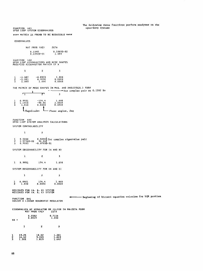
FUNCTION 401 OPEN LOOP SYSTEM EIGENVALUES

The following three functions perform analyses on the open-loop system:

Y Y Y Y MATRIX I S FOUND TO BE REDUCIBLE NYWY

EIGENVALUES

NAT FREQ (HZ) ZETA

0 . 1 5 9 2 0 . 1 5 9 2 D - 0 1 1 . 0 0 0

0 . 1 0 0 0 D - 0 2

OPEN LOOP EIGENVECTORS AND MODE SHAPES FUNCTION 4 0 2

MODIFIED EIGENVECTOR MATRIX OF A

1 2 3

2 - 1 . 0 0 1 1 - 1 . 0 8 7 - 0 . 8 9 3 3

0 . 9 9 9 0 1 . 0 0 0

0 . 0 0 0 0 3 1 . 0 0 0 1 . 0 0 0 0 . 0 0 0 0

THE MATRIX OF MODE SHAPES I N MAG. AND ANGLECDEG.) FORM

t For complex pair at 0.1592 HZ ' 1 2 ' 3

2 1 . 0 0 0 0 1 0 . 9 9 5 1 - 1 7 4 . 4 1 . 0 0 0

- 9 0 . 0 6 0 . 0 0 0 0 3 1 . 0 0 0 0 . 0 0 0 0 0 . 0 0 0 0

t Magnitudes Phase angles, deg

FUNCTION 403 OPEN LOOP SYSTEM ANALYSIS CALCULATIONS

SYSTEM CONTROLABILITY

1 2

2 0 . 5 7 3 0 D - 0 1 9 0 . 0 0 > 1 0 . 5 0 0 0 0 . 5 0 0 0 For complex eigenvalue pair 3 0 . 9 9 0 3 - 0 . 9 7 0 5 D - 0 1

SYSTEM OBSERVABILITY FOR ( A AND H)

1 2 3

1 0 . 9 9 5 1 1 7 4 . 4 1 . 0 0 0

SYSTEM OBSERVABILITY FOR ( A AND C)

1 2 3

2 1 . 0 0 0 1 0 . 9 9 5 1

0 . 0 0 0 0 1 7 4 . 4 1.000

0 . 0 0 0 0

RESIDUES FOR (A, B, H) SYSTEM RESIDUES FOR ( A , B, C ) SYSTEM

FUNCTION 8 0 1 DESIGN A LINEAR QUADRATIC REGULATOR

-Beginning of Riccati equation solution for LQR problem

EIGENVALUES OF REGULATOR OR F I L T E R I N F N I Z E T A FORM NAT FREQ (HZ) ZETA

0 . 2 3 8 2 0 . 4 5 1 9

0 . 7 1 1 6 1 . 0 0 0

ss =

I 2 3

1 1 9 . 2 4 2 1 0 . 4 2

1 0 . 4 2 1 . 3 0 1 9 . 2 0 3

3 1 . 3 0 1 1 . a 1 9 1 . 8 1 9 1 . 6 4 7

68

KC =

1 2 3

2 1.042 1 2.301 1.819

1.220 3.647

0.1819

FUNCTION a 0 2 STORE OPTIMAL CONTROL G A I N S ( K C ) ON U N I T 0 8 .

FUNCTION 3 0 1 FORM A-BKC MATRIX

FUNCTION 8 0 3 EIGENVALUES OF SYSTEM WITH STATE FEEDBACK

EIGENVALUES

NAT FREP (HZ1 ZETA

0.2382 0.4519

0 . 7 1 1 6 1.000

FUNCTION 804 EIGENVECTORS AND MODE SHAPES WITH STATE FEEDBACK

MODIFIED EIGENVECTOR MATRIX OF AMBKC

1 2 3

2 1.000 1 -0.9899 0 . 4 2 4 6 D - 0 1 0.1494

3 0.2144 -1.042 1 . 0 0 0 -0.4092

1.000

THE MATRIX OF MODE SHAPES I N MAG. AND ANGLECDEG.) FORM

1 2 3

2 1.000 1 0 . 7 0 0 6 -132.5

0 . 0 0 0 0 -0.4092 0.1494

3 0.7519 123.4 1.000 - Beginning of error checks for the Riccati solution matrix

FUNCTION 8 0 5 P O S I T I V E D E F I N I T E N E S S CHECK OF CONTROL RICCATI SOLUTION MATRIX , 55

EIGENVALUES

NAT FREQ (HZ) ZETA

0.1642 0.4929 Negative r indicates that eigenvalues all have positive real parts;

4 . 1 3 3 - 1 . 0 0 0 therefore SS is positive-definite

FUNCTION 806 SYMNETRY CHECK OF CONTROL RICCATI SOLUTIOH MATRIX . SS

MAX. SYMMETRY ERROR I N SS = -3.2429E-15 AVG. ABSOLUTE SYMMETRY ERROR I N S S = 1.7184E-15 SYMMETRY ERROR I N SS =

1 2 3

1 0.0000 2 -0.4475D-15 0.0000

0.0000 0 . 0 0 0 0

3 -0 .32431) -14 - 0 . 1 4 6 5 D - 1 4 0 . 0 0 0 0 0 . 0 0 0 0

FUNCTION 807 RESIDUAL ERROR CHECK OF SS

MAX. RESIDUAL, R( 1. 2)= - 0 . 2 8 4 2 D - 1 3

-0.2977D-13 TRACE OF RESIDUAL =

69

I

RESIDUAL ERROR MATRIX FOR CONTROL R I C C A T I E Q U A T I O N

1 2 3

1 -0.1421D-13 -0.2842D-13 -0.1577D-13 The residual remaining upon substitution of solution 2 -0.1754~-13 -0.16220-13 -o.a438~-14 3 -0.8882D-15 0.4441D-15 0.6661D-15 matrix SS back into the original Rlccati equation

FUNCTION a m STORE CONTROL R I C C A T I S O L U T I O N M A T R I X ( S S ) ON U N I T 16

-Beginning of Riccati equation solution for Kalman f i l t e r problem

DESIGN A KALMAN F ILTER FUNCTION a09

EIGENVALUES OF REGULATOR OR F I L T E R I N F N I Z E T A FORM NAT FREQ (HZ) ZETA

0.2202 1.000 0.2862 0.4451

PP =

1 2

4.442 11.76 1.865

3

8.865 18.37

1.462

1

STORE KALMAN F ILTER GAINS (KE) ON U N I T 09 FUNCTION 810

FUNCTION 302 FORM A-BKC-KEH MATRIX

FUNCTION a11 EIGENVALUES OF OPTIMAL CONTROLLER A-BKC-KEH

EIGENVALUES

NAT FREQ (HZ) ZETA

0.6057 1.000 0.5366 0.6000

FUNCTION 303 FORM ATOT, CTOT. DTOT, KCTOT. AND HTOT MATRICES FOR OPTIMAL CONTROL SYSTEM U I T H KALMAN F ILTER I N FEEDBACK LOOP

1 2 3 4 5 6

1 - 0 . 1 0 0 0 D 00 1.000 0.0000 0.0000 0.0000 2 0.0000 0.0000

0.0000

3 0.0000 1.000 -1.042 -1.220 -11.1619

-1.000 -0.2000D-02 -2.301 -1.819 0.0000

-3.647 -2.982

5 4.442 0.0000 6 1.482

0.0000 -5.484 0.0000 0.0000 -3.783 -2.819 -3.649

-1.220 ' 0.8181 4 2.862 0.0000 1.000 0.0000

CTOT =

1 2 3 4 5 6

1 1.000 2 0.0000

0.0000 0.0000 0.0000

0.0000 1.000

0.0000 -1.042

0.0000 -1.220 -0.1819

70

OTOT =

1 2

2 0 . 0 0 0 0 1 0 . 0 0 0 0

3 1 . 0 0 0 4 0 . 0 0 0 0 5 0 . 0 0 0 0 6 0 . 0 0 0 0

KCTOT

1

2 0 . 0 0 0 0 1 0 . 0 0 0 0

HTOT f

1

1 1 . 0 0 0

0 . 0 0 0 0 1 . 0 0 0

0 . 0 0 0 0 0 . 0 0 0 0 0 . 0 0 0 0 0 . 0 0 0 0

2 3

0 . 0 0 0 0 0 . 0 0 0 0 0 . 0 0 0 0 0 . 0 0 0 0

4 5 6

- 2 . 3 0 1 - 1 . 1 1 9 - 1 . 0 4 2

- 3 . 6 4 7 - 1 . 2 2 0 - 0 . 1 8 1 9

2 3 4 5 6

0 . 0 0 0 0 0 . 0 0 0 0 0 . 0 0 0 0 0 . 0 0 0 0 0 . 0 0 0 0

FUNCTION a 1 2 EIGENVALUES OF CONTROL SYSTEM WITH A FILTER I N THE FEEDBACK LOOP

EIGENVALUES

NAT FREQ ( H Z ) ZETA

0 . 2 2 0 2 0.2382

0 . 4 5 1 9 0 . 2 8 6 2

0 . 7 1 1 6 0 . 4 4 5 1 1.00u

1 . 0 0 0 These are the eigenvalues of A - KE H

These are the eigenvalues of A - B e KC

FUNCTION a 1 3 -Beginning of error checks on Kalman filter error covariance matrix

P O S I T I V E D E F I N I T E N E S S CHECK OF ERROR COVARIANCE MATRIX, PP

EIGENVALUES

NAT FREQ (HZ) ZETA

0 . 1 1 0 3

4 . 0 0 6 1 . 1 3 8

- 1 . 0 0 0

- 1 . 0 0 0 " a t r i x PP i s pos i t ive-def in i te

FUNCTION a 1 4 SYMMETRY CHECK OF ERROR COVARIANCE MATRIX, PP

MAX. SYMMETRY ERROR I N PP = - 2 . 9 9 6 2 E - 1 6 AVG. ABSOLUTE SYMMETRY ERROR I H PP = 1 . 6 6 6 7 E - 1 6 SYMMETRY ERROR I N PP =

1 2 3

1 0 . 0 0 0 0 2 0 . 0 0 0 0

0 . 0 0 0 0 0 . 0 0 0 0

0 . 0 0 0 0

3 - 0 . 2 9 9 6 D - 1 5 0 . 2 0 0 4 D - 1 5 0 . 0 0 0 0 0 . 0 0 0 0

FUNCTION a 1 5 RESIDUAL ERROR CHECK OF PP

MAX. RESIDUAL, R( 2. 2)' - 0 . 1 1 5 5 D - 1 3 TRACE OF RESIDUAL = - 0 . 2 2 6 5 D - 1 3

RESIDUAL ERROR MATRIX FOR ESTIMATION R ICCATI EQUATION

1 2 3

71

F U N C T I O N 8 1 6 STORE ERROR COVARIANCE MATRIX (PP) ON U N I T 15

COMPUTE COVARIANCE MATRICES FOR LINEAR QUADRATIC REGULATOR F U N C T I O N 8 1 7

WITH KALMAN FILTER I N FEEDBACK LOOP

UU. CONTROL COVARIANCE MATRIX

1 2

2 2 0 . 8 1 1 4 1 . 4 2 2 0 . 8 1

2 5 . 1 3

XX. STATE COVARIANCE MATRIX

1 2 3

1 2 0 . 9 9 2 . 0 9 9 2 2 . 0 9 9

- 6 . 8 4 9

3 - 6 . 8 4 9 2 1 . 5 6 8 . 4 2 8 8 . 4 2 8 2 4 . 2 6

YY. OUTPUT COVARIANCE MATRIX

1 2

1 2 0 . 9 9 - 2 1 . 3 5 2 - 2 1 . 3 5 6 5 . 6 7

ZZ, MEASUREMENT COVARIANCE MATRIX

1

1 2 0 . 9 9

FUNCTION 818 LYAPUNOV ERROR CHECK FOR F U N C T I O N 8 1 7 - Computes error incurred in calculating state covariance matrix xx THE T R A C E OF THE RESIDUAL" 0 . 6 5 1 4 8 ~ - 1 2 NORMALIZED DIAGONAL ELEFIENTS OF THE ERROR MATRIX = - 0 . 6 4 9 7 0 D - 1 5 0 . 6 3 0 5 1 D - 1 5 - 0 . 4 0 6 1 7 D - 1 4

THE TRACE OF THE COVARIANCE= 66.806 THE TRACE OF THE ERROR"0.98575D-13

TR(ERROR)/TR(COV.) =-0.14755D-14

FUNCTION 819 FORM FEED FORWARD MATRIX FOR NOH-ZERO SET POINT CONTROL

K F F =

1 2

F U N C T I O N 8 2 0 STORE FEED FORWARD MATRIX (KFF) ON U N I T 1 7

q- Beginning of frequency response and Bode plot computation

FUNCTION 5 0 1 OPEN LOOP FREQUENCY RESPONSE OF MEASUREMENT 1 TO CONTROL I N P U T 1

NUMERATOR COEFFICIENTS

- 0 . 1 2 0 8 9 D - l 6 * S Y Y 2 0 . 1 0 2 0 0 W S W W 2 1 . 0 0 0 0 wsrx 3

1 . 0 0 0 2 *sww 1 0 . 1 0 0 0 0 D O O W S W W 0

0 . 0 0 0 0 0 WSYY 3

0 . 0 0 0 0 0 rswx 1 1 . 0 0 0 0 Y S Y Y 0

DENOMINATOR COEFFICIENTS

72

I 1 111 I I 1 1 1 1 I

PLOT OPEN LOOP FREQ. RESPONSE OF MEASUREMENT TO CONTROL I N P U T FUNCTION 502

GRAPHICS DEVICE NOT DEFINED BY DDEF. ENTER U N I T NAPIE. DEFAULT TO CANCEL.

Z E T A 1 2 PLOT IDENTIFICATION = PELUCY** 02 DEC 1 9 8 2 a 0 8 : 0 6 : 1 a

-User s p e c i f i e s ZETA p l o t t e r to be used for plot t ing

F U N C T I O N 5 0 3 STORE OPEN LOOP FREQ. RESPONSE OF MEASUREMENT TO CONTROL I N P U T ON U N I T 1 0

FUNCTION 504 OPEN LOOP FREQUENCY RESPONSE OF OUTPUT 1 TO CONTROL I N P U T 1

NUMERATOR COEFFICIENTS

- 0 . 1 2 0 8 9 D - l 6 * S * * 2 0 . 1 0 2 0 0 * S * * 2 1 . 0 0 0 0 x s * * 3

1 . 0 0 0 2 *s * * 1 0 . 1 0 0 0 0 D O O * S X * 0

0 . 0 0 0 0 0 *s** 3

0 . 0 0 0 0 0 *s** 1 1 . 0 0 0 0 *sw* 0


FUNCTION 505 PLOT OPEN LOOP FREQ. RESPONSE OF OUTPUT TO CONTROL I N P U T

FUNCTION 506 STORE OPEN LOOP FREQ. RESPONSE OF OUTPUT TO CONTROL I N P U T ON U N I T 1 1

FUNCTION 507 OPEN LOOP FREQUENCY RESPONSE O F MEASUREMENT 1 T O DISTURBANCE INPUT 1

NUMERATOR COEFFICIENTS DENOMINATOR COEFFICIENTS 0 . 0 0 0 0 0 * S * * 3 1 . 0 0 0 0 *s*r 3

- 0 . 1 2 0 8 9 D - l 6 * S * X 2 0 . 1 0 2 0 0 * s * * 2 0 . 0 0 0 0 0 * s * * 1

1 . 0 0 0 0 *s** 0 0 . 1 0 0 0 0 D OOrS** 0 1 . 0 0 0 2 Y S * * 1

FUNCTION 508 PLOT OPEN LOOP FREQ. RESPONSE OF MEASUREMENT TO DISTURBANCE INPUT

FUNCTION 509 STORE OPEN LOOP FREQ. RESPONSE OF MEASUREMENT TO DISTURBANCE INPUT ON U N I T 1 2

FUNCTION 510 OPEN LOOP FREQUENCY RESPONSE OF OUTPUT 1 TO DISTURBANCE INPUT 1

NUMERATOR COEFFICIENTS DENOMINATOR COEFFICIENTS 0 . 0 0 0 0 0 *s*n 3 1 . 0 0 0 0 * s * * 3

- 0 . 1 2 0 8 9 D - l 6 * S * % 2 0 . 1 0 2 0 0 *s** 2 0.00000 * S * * 1

1 . 0 0 0 0 * S * * 0 0 . 1 0 0 0 0 D OO*S** 0 1 . 0 0 0 2 *s*w 1

PLOT OPEN LOOP FREQ. RESPONSE OF OUTPUT TO D I S T U R B A N C E I N P U l F U N C T I O N 5 1 1

F U N C T I O N 5 1 2 STORE OPEN LOOP FREQ. RESPONSE OF OUTPUT TO DISTURBANCE INPUT ON U N I T 1 3

F U N C T I O N 5 1 3 CLOSED LOOP FREQUENCY RESPONSE OF OUTPUT 1 TO DISTURBANCE INPUT 1 FOR STATE FEEDBACK

NUMERATOR COEFFICIENTS 8 . 0 0 0 0 0 * s * * 3

DENOMINATOR COEFFICIENTS 1 . 0 0 0 0 * S Y * 3

-0.22204D-15*;** 2 - 0 . 2 2 2 0 4 D - l 5 * S * x 1

. . . . . . .

0.81alo K S X W o

"""

4 . 9 6 9 3 *S* * 2

6 . 3 6 0 4 *S* * 0

"

8.2882 *s** 1

FUNCTION 514 PLOT CLOSED LOOP FREQ. RESPONSE OF OUTPUT TO DISTURBANCE INPUT FOR STATE FEEDBACK (PLUS THE CORRESPONDING OPEN LOOP RESPONSE, I F DESIRED)

FUNCTION 515 CLOSED LOOP FREQUENCY RESPONSE OF CONTROL 1 TO DISTURBANCE INPUT 1 FOR STATE FEEDBACK

NUMERATOR COEFFICIENTS 0 . 0 0 0 0 0 * S * * 3 1 . 0 0 0 0 *S** 3 - 3 . 6 4 7 0 *S*W 2 4 . 9 6 9 3 * S X * 2


- 6 . 3 0 3 4 XSWW 1 - 6 . 2 7 6 3 *S** 0

13

FUNCTION 5 1 6 PLOT CLOSED LOOP FREQ. RESPONSE OF CONTROI TO DISTURBANCE INPUT FOR STATE FEEDBACK

FUNCTION 5 1 7 CLOSED LOOP FREQUENCY RESPONSE OF MEASUREMENT 1 TO DISTURBANCE INPUT 1 FOR CONTROL SYSTEM WITH A F I L T E R I N THE FEEDBACK LOOP

NUMERATOR COEFFICIENTS 0 . 0 0 0 0 0 Y S Y Y 6

DENOMINATOR COEFFICIENTS 1 . 0 0 0 0 Y S X Y 6

0 . 0 0 0 0 0 W I W W 4 - . - - - . -

1 . 0 0 0 0 YSWW 3 7 . 8 5 1 6 rSw* 2 2 6 . 7 6 4 X S r Y 1 4 3 . 2 6 3 *S*W 0

2 8 . 5 6 6 Y S Y Y 4 6 2 . 6 3 9 *S*X 3

. ..."

FUNCTION 5 1 8 PLOT CLOSED LOOP FREQ. RESPONSE OF MEASUREMENT TO DISTURBANCE INPUT FOR CONTROL SYSTEM U I T H F I L T E R I N FEEDBACK LOOP (PLUS THE CORRESPONDING OPEN LOOP RESPONSE, I F DESIRED)

CLOSED LOOP FREQUENCY RESPONSE OF OUTPUT 1 TO DISTURBANCE INPUT 1 FUNCTION 5 1 9

FOR CONTROL SYSTEM WITH A F I L T E R I N THE FEEDBACK LOOP

NUMERATOR COEFFICIENTS 0 . 0 0 0 0 0 Y S Y Y d

DENOMINATOR COEFFICIENTS 1 . 0 0 0 0 X S Y X 6

0 . 0 0 0 0 0 W S Y X 5 0 . 0 0 0 0 0 rsrr 4

7 . 8 5 1 6 X S * * 2 1 . 0 0 0 0 ws** 3

2 6 . 7 6 4 W S X X 1 4 3 . 2 6 3 Y S X X 0

7 . 9 5 3 6 rSrw 5 2 8 . 5 6 6 Y S w w 4

8 6 . 3 6 2 Y S Y Y 2 6 2 . 6 3 9 X S X X 3

7 1 . 7 2 5 Y S X Y 1 2 8 . 4 5 2 XSWX 0

PLOT CLOSED LOOP FREQ. RESPONSE OF OUTPUT TO DISTURBANCE INPUT FUNCTION 520

FOR CONTROL SYSTEM WITH FILTER I N FEEDBACK LOOP (PLUS THE CORRESPONDING OPEN LOOP RESPONSE, I F DESIRED)

FUNCTION 521 CLOSED LOOP FREQUENCY RESPONSE OF CONTROL 1 TO DISTURBANCE INPUT 1 FOR CONTROL SYSTEM WITH A F I L T E R I N THE FEEDBACK LOOP

NUMERATOR C O E F F I C I E N T S

-0.44409D-15YSxX 5 0 . 0 0 0 0 0 Y S Y X 6

-0 .13323D-14XSxr 4 - 0 . 3 9 9 6 8 D - l 4 * S * * 3

DENOMINATOR COEFFICIENTS 1 . 0 0 0 0 Y S Y X 6 7 . 9 5 3 6 US** 5

62 .63 '1 Y S X Y 3 2 8 . 5 6 6 Y S X Y 4

- 2 0 . 1 1 7 sS*Y 2 8 6 . 3 6 2 * 5 x * 2 - 6 . 8 3 1 5 rSr* 1 - 2 4 . 0 8 8 Y S w X 0 2 8 . 4 5 2 * S X * 0

7 1 . 7 2 5 XSWX 1

FUNCTION 522 PLOT CLOSED LOOP FREQ. RESPONSE OF CONTROL TO DISTURBANCE INPUT FOR CONTROL SYSTEM WITH F ILTER I N FEEDBACK LOOP

FUNCTION 5 2 3 FREQUENCY RESPONSE OF CONTROL

FOR OPTIMAL CONTROLLER

NUMERATOR C O E F F I C I E N T S 0 . 0 0 0 0 0 Y S W Y 3 - 2 0 . 1 1 7 YSWY 2

- 2 4 . 0 8 8 YSNY 0 - 6 . 8 3 1 5 XSWW 1

FUNCTION 5 2 4 PLOT FREQ. RESPONSE OF CONTROL FOR OPTIMAL CONTROLLER

1 TO MEASUREMENT 1

DENOMINATOR COEFFICIENTS 1 . 0 0 0 0 * S * * 3 7 . 8 5 1 6 W S X Y 2 2 6 . 7 6 4 Y S % X 1 t 3 . 2 6 3 X S Y Y 0

TO MEASUREMENT

FUNCTION 525 STORE FREQ. RESPONSE OF CONTROL TO MEASUREMENT FOR OPTIMAL CONTROLLER ON U N I T 1 4

--&ginning of transient response calculations and plots FUNCTION 6 0 1 OBTAIN AND PLOT SELECTED OPEN LOOP STEP RESPONSES

S T A T E T R A N S I T I O N M A T R I X FOR OPEN LOOP SYSTEM FOR T I M E S T E P = 0 . 5 0 0 0 D - 0 1

74

1 2 3

1 0.9950 0.4985D-01 0.1248D-02 2 0 . 0 0 0 0 0.9938 3 0.0000 -0.49980-01 0.9987

0.4993D-01

FORCED RESPONSE MATRIX OF OPEN LOOP SYSTEM FOR T IME STEP -0.50000-01

1 2 3

1 0.49a8~-01 O . ~ Z ~ ~ D - O Z 0 . 2 0 8 0 D - 0 4 2 0 . 0 0 0 0 3 0.0000 -0.1250D-02 0.4998D-01

0.4998D-01 0.125OD-02

FUNCTION 602 O B T A I N A N 0 P L O T S E L E C T E D I N I T I A L C O N D I T I O N RESPONSES FOR THE OPEN LOOP SYSTEM

STATE TRANSIT ION MATRIX FOR OPEN LOOP SYSTEM FOR T IME STEP -0.5000D-01

1 2 3

2 0.0000 1 0.9950 0.49a5~-01 0.1248~-02

0.9988 3 0.0000 -0.49980-01 0.9987

0.4998D-01

FORCED RESPONSE MATRIX OF OPEN LOOP SYSTEM FOR T IME STEP =0.5000D-01

1 2 3

1 0.4988D-01 0.124813-02 0.2080D-04 2 0.0000 3 0.0000 -0.1250D-02 0.499SD-01

0.4998D-01 0.1250D-02

O B T A I N AND PLOT SELECTED I N I T I A L C O N D I T I O N RESPONSES FUNCTION 603

FOR THE CLOSED LOOP LINEAR REGULATOR

STATE TRANSITION MATRIX OF LINEAR REGULATOR FOR T IME STEP 0.5000D-01

1 2 3

2 -0.5251D-01 0.9369 1 0.9937 0.4832D-01 0.9413D-03

0.3619D-01 3 -0.1014 -0.1273 0.8307

FORCED RESPONSE MATRIX OF LINEAR REGULATOR FOR T IME STEP 0.5OOOD-01

1 2 3

1 0.49850-01 0.1222D-02 0.1602D-04 2 -0.1310D-02 0.4844D-01 O.9429D-03 3 -0.2645D-02 -0.3294D-02 0.4566D-01

FUNCTION 604 O B T A I N AND PLOT SELECTED STEP RESPONSES FOR THE NON-ZERO SET POINT LINEAR REGULATOR

.STATE TRANSITION MATRIX OF LINEAR REGULATOR FOR T IME STEP 0.50000-01

1 2 3

1 0.9937 0.48321)-01 0.94130-03 2 -0.52510-01 0.9369 3 -0.1014 -0.1273

0.3619D-01 o .a307

FORCE0 RESPONSE MATRIX OF LINEAR REGULATOR FOR TIME STEP 0.5000D-01

1 2 3

1 0.49a5~-01 0.12220-02 0.16020-05 2 -0.1310D-02 0.4844D-01 0.94290-03 3 -0.2645D-02 -0.32940-02 0.4566D-01

75

- Beginning of transfer function gain and numerator zeros calculation FUNCTION 7 0 1 G A I N AND ZEROES OF OPEN LOOP TRANSFER FUNCTION RELATING MEASUREMENT 1 TO CONTROL I N P U T 1

G A I N = 1 . 0 0 0 0 0 NUMBER OF ZEROES = 0 REAL PARTS OF NUMERATOR ZEROES

1

1 0 . 0 0 0 0

IMAGINARY PARTS OF NUMERATOR ZEROES

1

1 0 . 0 0 0 0

FUNCTION 7021 G A I N AND ZEROES OF OPEN LOOP TRANSFER FUNCTION RELATING OUTPUT 1 TO CONTROL INPUT 1

G A I N 5 1 . O O U O O

NUMBER OF ZEROES = 0 REAL PARTS OF NUMERATOR ZEROES

1

1 0 . 0 0 0 0


1

1 0 . 0 0 0 0

FUNCTION 703 G A I N AND ZEROES OF OPEN RELATING MEASUREMENT 1

G A I N 1 . 0 0 0 0 0 NUMBER OF ZEROES = 0 REAL PARTS OF NUMERATOR

LOOP TRANSFER FUNCTION TO DISTURBANCE INPUT 1

ZEROES

1

1 0 . 0 0 0 0


1

1 0 . 0 0 0 0

G A I N AND ZEROES OF OPEN LOOP TRANSFER FUNCTION FUNCTION 7 0 4

RELATING OUTPUT 1 TO DISTURBANCE INPUT 1

G A I N = 1 . 0 0 0 0 0

REAL PARTS OF NUMERATOR ZEROES NUMBER OF ZEROES = 0

1

1 0 . 0 0 0 0


1

1 0 . 0 0 0 0

76

F U N C T I O N 7 0 5 G A I N AND ZEROES OF OPTIMAL CONTROLLER TRANSFER FUNCTION RELATING CONTROL 1 T O MEASUREMENT 1

G A I N 2 0 . 1 1 7 0 NUMBER OF ZEROES 2 REAL PARTS OF NUMERATOR ZEROES

1

1 - 0 . 1 6 9 9 2 - 0 . 1 6 9 9


1

2 - 1 . 0 8 1 1 1.oa1

Beginning of series of functions that demonstrate (1) normalizing of input matrices, - matrices, and (4) unnormalizing KC, KE, KFF, and PP to show that results are ( 2 ) normalizing of control weighting matrices, (3) recomputing of KC, KE, and KIT

FUNCTION 210 identical to prior calculations CHANGE MATRICES A, B. C. D, H, DOUT, CSP, QC, NN, PCINV, QQ, OR RRINV AND !NY OR ALL DIMENSIONS BY READING CHANGES I N AT TERMINAL USING NAMELIST 'MATDAT DISPLAY MATDAT BEFORE MAKING CHANGCS? Y (MATDAT A: -0 . lOD0, 49W0.0 . 1 .0 . 0 . 0 . - 1 . 0 , 4 8 W 0 . 0 . 1 . 0 , -0.20D-02. 2397W0.0

D= 2WO.O. 1 . 0 , 48360.0, 1 .0 , 698W0.0 C= 1 .0 , 100M0.0 , 1 .0 , 2398WO.O

H Z 1 . 0 , 249WO.O DOUT- 51W0.0, 1.0, 198WO.O

QC= 20.0, 5 0 X 0 . 0 , 1 . 0 . 5 0 W 0 . 0 , 10.0, 2397WO.O CSP- 1 .0 , 10WO.O. 2.0, 238WO.O

NN= 1 . 0 , 0 . 0 , 2 . 0 . 4 8 W 0 . 0 , 3.0. 198WO.O PCINVZ 1 .0 , 5 W O . O . 0.10DO. 1SWO.O Q Q = 51WO.O. 2 .0 , 50W0.0 , 20.0. 2397WO.O R R I N V - 1 . 0 , 24WO.O N= 3 NM= 1 NC= 2 ND= 2 N O = 2 &END ENTER MATDAT CHANGES AS LMATDAT A ( 1 , 1 ) = . ETC. LEND

B = 2 ~ 0 . 0 , 1.0. 4axo.0, 1.0, 1 9 a ~ o . o

a M b r n d r -. ._. . 1 1 1 ,

QC(2.2) 9.ODO QC(1.1) = 500.ODO QC(3.3) 40.ODO P C I N V ( 1 , l ) 1 . 5 6 2 5 D - 2 P C I N V ( 2 . 2 ) = 1 . 2 3 4 5 6 7 9 D - 3 N N ( 1 . 1 ) 40.ODO N N ( 3 . 1 ) 32.ODO N l i ( 2 . 2 ) = 8 1 . 0 0 0 LEND

-New values for weighting elements calculated off-line so

stored above as MATDAT that they correspond to normalized versions of those

P M A T n A l -. . . . . -. . . A = - 0 . 1 0 ~ 0 . 4 9 ~ 0 . 0 , 1.0, 0 . 0 . -1.0, 4aro.o. 1.0, -0.20~-

D= 2~0.0. 1.0. 4awo.o. 1.0. 6 9 8 ~ 0 . 0

B = 2W0.0. 1 . 0 , 48WO.O. 1.0, 198WO.O C= 1 .0 , 100WO.O. 1.0, 2398WO.O

RRINV= 1.0, 2 4 ~ 0 . 0 N = 3

.02, 2397WO. 0

FUNCTION 4 0 4 NORMALIZE SYSTEM MATRICES; NORMALIZING FACTORS ARE READ I N FROM U N I T 34 I F NOT PREVIOUSLY SET

I F NOT ALREADY DONE. DDEF DATASET CONTAINING HAMELIST 'HRMS' TO UNIT 34 PROCEEDING: PAUSE . PROGRAM W I L L PROCEED I F -RUN CDMMAND ISSUED.

DDEF FT34FOOl.VS.ANRMS

GO PROCEEDING(PCS): EXECUTION CONTINUES AT CHCRWC.(X'4CD4')

NORMALIZING FACTORS ARE fHRMS SCXZ 5.0, 3 . 0 . 2.0. 47WO.O SCUD 1.0. 9.0. 3xo.o

77

SCY' 4 . 0 , 7 . 0 . 1 0 . 0 , 47XO.O SCZ' 6 . 0 , 4 X 0 . 0 SCYSPZ 1 2 . 0 , 1 1 . 0 , 3r0.0 &END

NORMALIZED SYSTEM MATRICES

THE A MATRIX I S

1 2

2 0 . 0 0 0 0 1 - 0 . 1 0 0 0 D 0 0 0.6000

3 0.0000 0.0000 - 1 . 5 0 0

THE B MATRIX I S

1 2

1 0 . 0 0 0 0 2 0 . 0 0 0 0

0 . 0 0 0 0

3 4 . 0 0 0 0.0000 3 . 0 0 0

THE C MATRIX I S

1 2

1 1 . 2 5 0 2 0 . 0 0 0 0 0 . o a a o

0.0000

THE H MATRIX I S

1 2

1 0 . 8 3 3 3 0.0000

THE Q Q MATRIX I S

1 2

2 0 . 0 0 0 0 1 0 . 0 0 0 0 0.0000

0 . 2 2 2 2 3 0.0000 0.0000

THE RRINV MATRIX I S

1

1 3 6 . 0 0

THE D MATRIX I S

1 2

1 0.0000 2 0 . 0 0 0 0 0 . 3 3 3 3

0 . 0 0 0 0

3 0 . 5 0 0 0 0 . 0 0 0 0

THE DOUT MATRIX I S

1 2

2 0 . 0 0 0 0 1 0 . 0 0 0 0 0 . 0 0 0 0

1 . 2 8 6

THE CSP MATRIX I S

1 2

1 0 . 4 1 6 7 0 . 0 0 0 0 2 0 . 0 0 0 0 0.0000

3

0.0000 0.6667

-0 .2000D-02

3

0 . 2 8 5 7 0 . 0 0 0 0

3

0 . 0 0 0 0

3

0.0000 0.0000 5.000

3

0 . 0 0 0 0 0 . 3 6 3 6

DESIGN A LINEAR QUADRATIC REGULATOR FUNCTION 801

I8

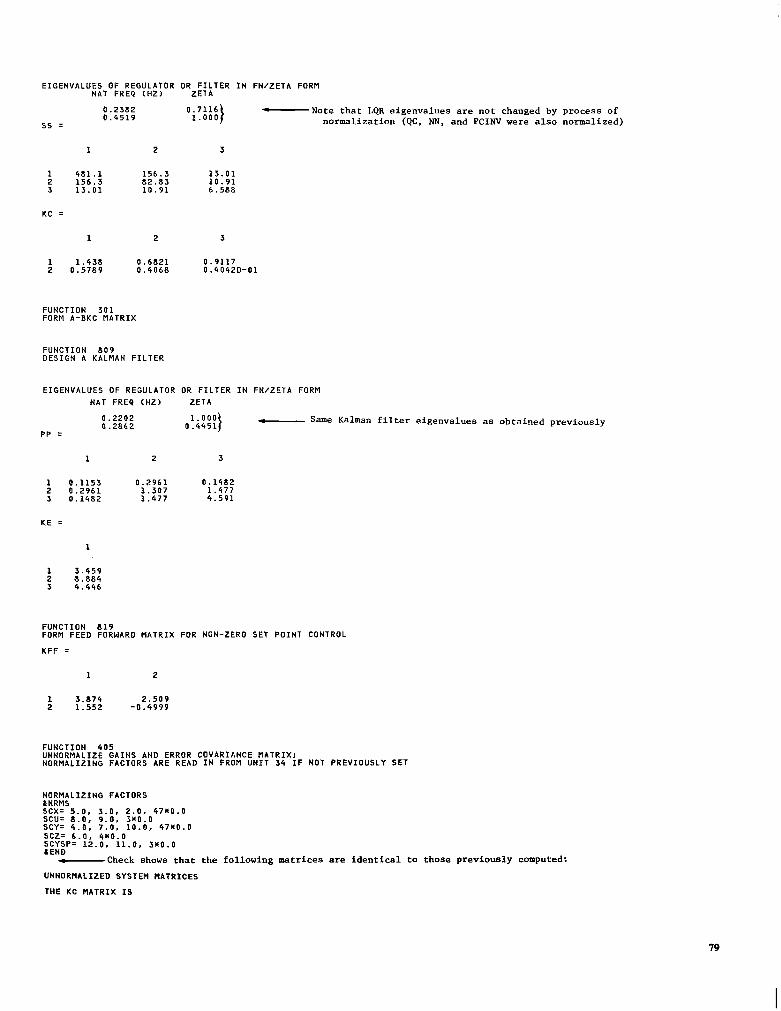
EIGENVALUES OF REGULATOR OR F I L T E R I N F N / Z E T A FORM NAT FREQ (HZ) ZETA

0.2382 0.4519

0.7116 -Note that LQR eigenvalues are not changed by process of 1.000)

ss = normalization (QC, NN, and PCINV were also normalized)

1 2 3

2 156.3 1 481.1 156.3 13.01

3 13.01 10.91 6.588 10.91 82.83

1 2 3

2 0.5789 1 1.438 0.6821 0.9117

0.4068 0.4042D-01

FUNCTION 301 FORM A-BKC MATRIX

FUNCTION 809 DESIGN A KALMAN F ILTER

EIGENVALUES OF REGULATOR OR F I L T E R I N F N I Z E T A FORM NAT FREP (HZ) ZETA

1 2 3

1 0.1153 2 0.2961

0.2961 0.1482

3 0.1482 1.307 1.477

1.477 4.591

K E :

1

1 3.459 2 8.884 3 4 . 4 4 6

FUNCTION 019 FORM FEED FORWARD MATRIX FOR NON-ZERO SET POINT CONTROL

K F F =

1 2

1 3.074 2 1.552 -0.4999

2.509

FUNCTION 405 UNNORMALIZE GAINS AND ERROR COVARIANCE MATRIX; NORMALIZING FACTORS ARE READ I N FROM U N I T 34 I F NOT PREVIOUSLY SET

NORMALIZING FACTORS LNRMS S C X = - 5 . 0 , 3.0, 2.0, 47360.0 SCU: 8 . 0 , 9.0, 3W0.0 SCY: 4 . 0 . 7.0, 10.0, 47K0.0 SCZ: 6.0, 4WO.O SCYSPZ 12.0, 11.0, 3360.0 &END

-Check shows that the following matrices are identical to those previously computed:

UNNORMALIZED SYSTEM MATRICES

THE KC MATRIX I S

79

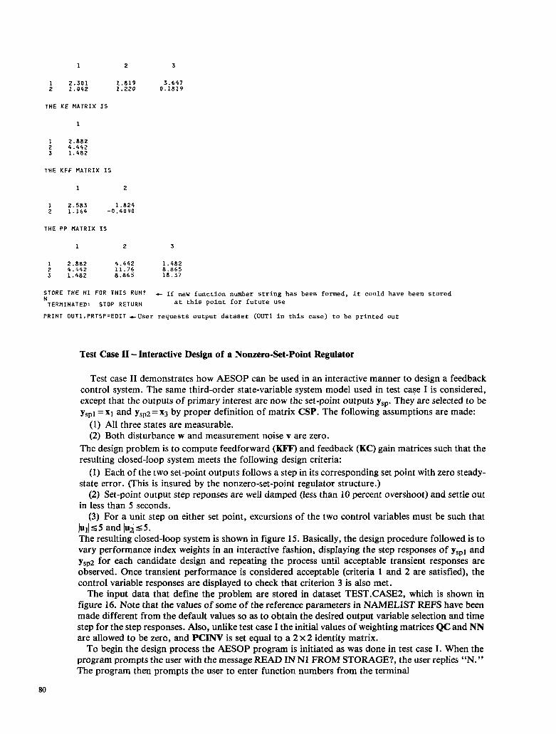
1 2 3

1 2.301 2 1.042

1.819 1.220 0.1819

3 . 6 4 7

THE KE M A T R I X IS

1

2 4.442 3 1.482

1 2.082

THE KFF MATRIX IS

1 2

1 2.583 1.824 2 1.164 - 0 . 4 0 9 0

T H E PP MATRIX I S

1 2 3

2 4.442 1 2.882 4 . 4 4 2 1.482

3 1.482 11.76 8.865 8.865 la. 37

STORE THE N 1 FOR THIS R U N ? c If new function number s t r ing has been formed, i t could have been stored N

T E R M I N A T E D : STOP R E T U R N a t t h i s po in t for fu ture use

PRINT OUTl,PRTSP=EDIT+User requests output dataset (OUT1 i n th i s case) to be p r in ted ou t

Test Case I1 - Interactive Design of a Nonzero-Set-Point Regulator

Test case I1 demonstrates how AESOP can be used in an interactive manner to design a feedback control system. The same third-order state-variable system model used in test case I is considered, except that the outputs of primary interest are now the set-point outputs ysp. They are selected to be yspl =x1 and ysp2=x3 by proper definition of matrix CSP. The following assumptions are made:

(1) All three states are measurable. (2) Both disturbance w and measurement noise v are zero.

The design problem is to compute feedforward (KFF) and feedback (KC) gain matrices such that the resulting closed-loop system meets the following design criteria:

(1) Each of the two set-point outputs follows a step in its corresponding set point with zero steady- state error. (This is insured by the nonzero-set-point regulator structure.)

(2) Set-point output step reponses are well damped (Iess than 10 percent overshoot) and settle out in less than 5 seconds.

(3) For a unit step on either set point, excursions of the two control variables must be such that JulJs5 and bd55. The resulting closed-loop system is shown in figure 15. Basically, the design procedure followed is to vary performance index weights in an interactive fashion, displaying the step responses of yspl and ysp2 for each candidate design and repeating the process until acceptable transient responses are observed. Once transient performance is considered acceptable (criteria 1 and 2 are satisfied), the control variable responses are displayed to check that criterion 3 is also met.

The input data that define the problem are stored in dataset TEST.CASE2, which is shown in figure 16. Note that the values of some of the reference parameters in NAMELIST REFS have been made different from the default values so as to obtain the desired output variable selection and time step for the step responses. Also, unlike test case 1 the initial values of weighting matrices QC and NN are allowed to be zero, and PCINV is set equal to a 2 x 2 identity matrix.

To begin the design process the AESOP program is initiated as was done in test case I. When the program prompts the user with the message READ IN N1 FROM STORAGE?, the user replies “N.” The program then prompts the user to enter function numbers from the terminal

80

0 4 8 8 9 0 0 0 4 8 9 0 0 0 0 4 8 9 1 0 0 0 4 8 9 2 0 0 0 4 8 9 3 0 0

0 4 8 9 5 0 0 0 4 8 9 4 0 0

0 4 8 9 7 0 0 0 4 8 9 6 0 0

0 4 8 9 8 0 0 0 4 8 9 9 0 0

Figure 15. - Nonzero-set-point regulator.

Figure 16. -Data for test case 11, contained in dataset TEST.CASE2.

ENTER NAMELIST DATA AS '&N1 IFN = , , , &END

and the user responds with

&nl ifn = 202,203,801 &end

The user then datadefs dataset TEST.CASE2 to unit 33.

FUNCTION 202 READ INPUT DATA -- MATRICES AND REFERENCE VALUES DEFINED IN NAHELIZTS 'PIATDAT' AND 'REFS'

IF NOT ALREADY DONE9 DDEF DATASET CONTAINING NAMELISTS

CHCRU410 'HATDAT' AND 'REFS' TO UNIT 33

PROCEEDING: PAUSE ddef ft33COOl~vsrtest.case2 90 CZAPB030 DISPLAY INPUT MATRICES?

PROCEEDING(FCS): EXECUTION CONTINUES A'l' CHCKUCt(X'4CD4')

n

The next requested function (203) allows the user to enter desired performance index weights. For this test case, weights on the two controls will be fixed at unity and the weight on state 1 will be varied. A low value (0.001) is selected initially, and the program proceeds to compute an LQR solution.

FUNCTION 203 DISPLAY CONPAR BEFORE MAKING CHANGES? Y ZCONPAR QC= 2SOO%O.O NN= 250%0.0

81

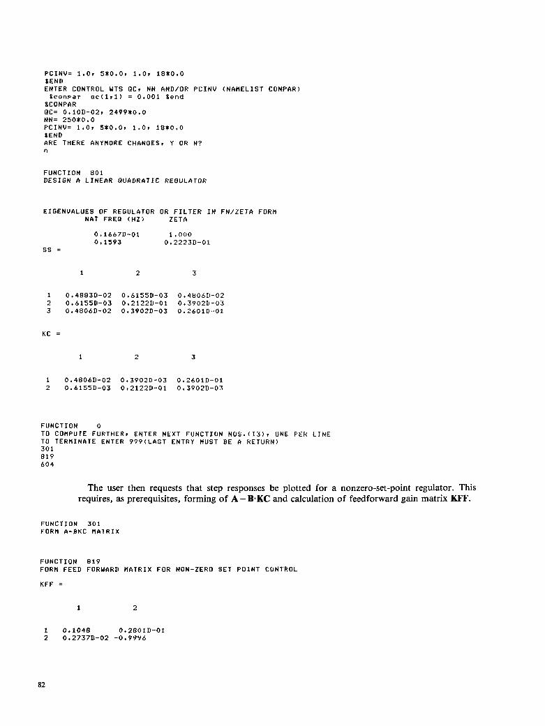
PCINU= 1.0, 5 $ 0 + 0 , 1.0, 18$0.0 PEND ENTER CONTROL UTS RCI N N AND/OR PCINU (NAMELlST CONPAR)

LCONPAR

N N = 250*0 .0 QC= 0.10D-029 2499$0.0

PCINU= 1 . 0 , 5$0.0~ 1.01 18$0.0 LEND

n

Lconpar ac(lr1) = 0.001 tend

ARE THERE ANYMORE CHANGES, Y OR N?

FUNCTION 801 DESIGN A LINEAR QUADRATIC REGULATOR

EIGENVALUES OF REGULATOR OR F I L T E R I N F N / Z E T A FORM NAT FREQ (HZ) ZETA

0.1667D-01 1.000 0,1593

ss = 0 s 2223D-01

1 2 3

KC =

1 2 3

FUNCTION 0

TO TERMINATE ENTER 999(LAST ENTRY MUST BE A RETURN) 301 819 604

TO COMPUTE FURTHERt ENTER NEXT FUNCTION NOS*(IY)t ONE F E R L I N E

The user then requests that step responses be plotted for a nonzero-set-point regulator. This requires, as prerequisites, forming of A-B-KC and calculation of feedforward gain matrix KFF.

FUNCTION 301 FORM A-BKC M A l R I X

FUNCTION 819 FORM FEED FORWARD h A T R I X FOR NON-ZERO SET P U l N T CONTROL

K F F =

1 2

1 0.1048 0.2801D-01 2 0 273711-02 -0 + 9996

82

F U N C T I O N 604 O B T A I N AND PLOT SELECTEI I STEF ' RESPONSES F O R T H E N O N - Z E R O S E T P O I N T L I N E A R R E G U L A T O R

S T A T E T R A N S I T I O N H A T R I X OF L I N E A R R E G U L A T O R F O R T I N E S T t P 0 , 2 4 0 0

1 2 3

1 0.9763 0.2343 0,2831D-01 2 -0.2602D-03 0.9664 0 2362 3 -0.1108D-02 -0,2365 0.9648

F O R C E D R E S P O N S E H A T R I X OF L I N E A R R E G U L A T O R F O R T I M E S T E P 0 .2400

1 2 3

1 0.2371 0.2839Cl-01 0 * 227611-02 2 -0.284111-04 0.2371 3 -0.1349D-03 -0.2857D-01 0.2369

0.2854Ib"l

Next, before plots can be obtained, the user must indicate on which device the plots are to be generated by entering the user's terminal number (LAOOI), indicating that plots are to be displayed not on an off-line device but at the user's terminal.

G R I N T l O O G R A P H I C S D E V I C E N O T D E F I N E D BY D D E F . E N T E R U N I T N A H E . D E F A U L T TO C A N C E L .

la011

Two plots are then displayed: one for the response of yspl to a step in Yspdly and the other for ysp2 to a step in Yspd2-

83

1 . I

0.'

0.1

0.;

,-. O.(

- v 0.t

a ln >

0.'

0.3

0.2

0.1

S T E P R E S P O N S E S F O R N O N - Z E R O S E T - P O I N T R E G .

I N P U T : S E T P O I N T C O M M A N D Y S P D ( 1 4 M P L I T U O E = 1 - 0 0

DEC 7 3 I982 RUN NO. 3

STEP RESPONSES FCR NON-ZERO S E T - P O I N T REG. I N P U T : SET P O I N T COMMAND YSPO ( 2 1

A n P L I T U o E = 1 .oo DEC 7 s I982 RUN NO. 3 2 . 0 -

1.. 8 -

1 . 6 -

1 . Y -

1 . 2 - ‘u

.2 1 .0 - a VI %

0 . 8 -

0.6 -

0.4 --

0 . 2 ”

0.9 I I I I I I I I I I 0.0 2 . 5 5 . 0 7 . 5 10.0 1 2 . 5 15.0 17 .5 20.0 2 2 . 5 2 5 . 0

85

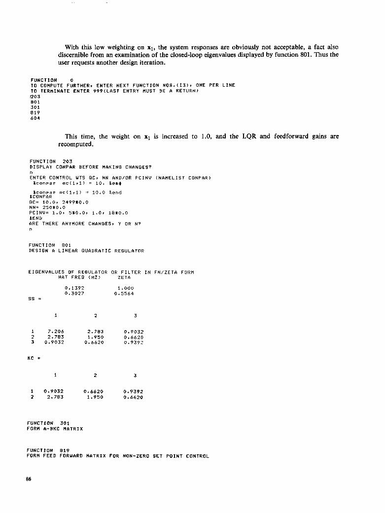
With this low weighting on XI, the system responses are obviously not acceptable, a fact also discernible from an examination of the closed-loop eigenvalues displayed by function 801. Thus the user requests another design iteration.

TO COBPUTE FURTHER, ENTER NEXT FUNCTION N O S + ( 1 3 ) r ONE PER L I N E FUNCTION 0

2 0 3 TO TERf l INATE ENTER 999(LAST ENTRY MUST HE A RETURN)

8 0 1

8 1 9 3 0 1

6 0 4

This time, the weight on x1 is increased to 1.0, and the LQR and feedforward gains are recomputed.

FUNCTION 203 D ISPLAY CONPAR BEFORE BAtiING CHANGES? n ENTER CONTROL WTS RC, NN AND/OR PCINU (NAMELIST CONFAR) Lconrar c+c(lrl) = 10. gem#

Lconpar nc(1rl) = 10.0 Zend LCUNPAR Q C = 1 0 . 0 , 2 4 9 9 t O . O NN= 2 5 0 t 0 . 0 FCINU= 1.0. 5t0.0, 1 . 0 , 18tO.O LEND ARE THERE ANYMORE CHANGES9 Y OR N? n

F U N C T I O N 8 0 1 DESIGN A LINEAR QUADRATIC REGULATOR

EIGENVALUES O F REGULATOR OR F I L T E R I N F N / Z E T A FORM NAT FREQ (HZ) ZETA

0 , 1 3 9 2 1 . 0 0 0 0 . 3 0 2 7 0.5564

ss =

1 2

1 7 . 2 0 6 2 . 7 8 3 2 2 . 7 8 3 3 0 . 9 0 3 2

1 , 9 5 0 0 t 6 6 2 0

KC =

1 2

1 0 . 9 0 3 2 0 t 6 6 2 0 2 2 . 7 8 3 1 . 9 5 0

F U N C T I O N 3 0 1 FORB A-RKC MATRIX

3

0 9 0 3 2 0 6620 0 . 9 3 9 2

3

0 * 9 3 9 2 0 t 6 6 2 0


86

K F F =

1 2

2 2.978 1 1.069 0,9412

-0 3380

F U N C T I O N 604 O B T A I N A N D P L O T S E L E C T E P S T E P R E S P O N S E S F O R T H E N O N - Z E R O S E T P O I N T L I N E A R R E G U L A T O R

S T A T E T R A N S I T I O N M A T R I X O F L I N E A R R E G U L A T O R F O R T I M E STEP 0.2400

1 2 3

1 0.9089 0.1832 0+7571D-02 2 -0.5167 0.5573 0.5555D-01 3 -0.8230D-01 -0.2934 0.7855

F O R C E D R E S P O N S E M A T R I X O F L I N E A R R E G U L A T O R F O R T I M E S l E P 0.2400

1 2 3

1 0.2315 0.2420D-01 0.646911-03 2 -0,6794D-01 0.1856 0 763611-02 3 -0.1475D-01 -0.3928D-01 0.2138

Now, the damping ratio of the complex eigenvalue pair has increased to 0.388, which is still too small to give acceptably damped responses. This fact is confirmed by the set-point responses, which are displayed next.

87

2.0

1. . 8

1 . 6

1.4

,. 1.2

c

v 1 . 0

a 07 *

0.8

0.6

0.4

0.2

0.0 a

STEP RESPONSES FOR NON-ZERO SET-POINT REG. I N P U T : S E T P O I N T COMMAND YSPD ( 1 )

A M P L I T U D E = 1 .oo OEC 7 n I982 RUN NO. 3

88

2.0

1 . 8

1 . 6

l . Y

n 1 . 2

N

v 1 . 0

a vr %

0.8

0 . 6

0.Y

0.2

STEP RESPONSES FOR NON-ZERO SET-POINT REG. INPUT: SET POINT COMMANO YSPD ( 2 )

4MPLITUDE = 1 .oo DEC 7 9 I982 RUN NO. 3

TIME

89

Actually, the IO-percent overshoot criterion is met, but yspl does not quite reach steady state in less than 5 seconds. Thus the user begins a third design iteration, choosing the weighting on x1 to be 10 this time.

FUNCTION 0 TO COMPUTE FURTHER, EN TO TERMINATE ENTER 999

801 203

819 30 1

604

TER NEXT ( L A S T E N

F U N C T I O N N U S . ( I ( l ) r ONE F t R L I N E TRY MUST HE A RETURN)

FUNCTION 203 D I S P L A Y CONPAR BEFORE MAtiING CHANGES? n ENTER CONTROL WTS OC, N N AND/OR PCINV (NAMELIST CONFAR)

SCONPAR OC= 1.0, 2499$0.0 NN= 250XO.O

SEND ARE THERE ANYMORE CHANGES, Y OR N? n

PCINU= 1 . 0 1 5X0.0, 1 .0 , 18*0 .0

FUNCTION 801 DESIGN A LINEAR QUADRATIC REGULATOR

EIGENVALUES OF REGULATOR OR F I L T E R I N F N I Z E T A FORfl NAT FREO ( H Z ) ZETA

0+952411-01 1.000 0 2063 0 3879

The preceding eigenvalues indicate that response time should now be acceptable as the slowest eigenvalue (A1 = 0.1392 Hz = 0.875 rad/sec) should give a settling time ( - 4/Al) of about 4.5 seconds.

ss =

1 2

1 1.285 0.6844 2 0.6844 3 0.5240 0.3449

0 + 7483

tic =

1 2

1 0.5240 0 3449 2 0.6844 0.7483

FUNCTION 301 FORM A-HtiC MATRIX

3

0.5240

0 + 7536 0 + 3449

3

0,7536 0,3449


90

KFF =

1 2

1 0 . 6 5 8 5 0 .7556 2 0 . 7 5 9 2 -0 6551

F U N C T I O N 604 O B T A I N A N D P L O T S E L E C T E D S T E P R E S P O N S E S FOR T H E N O N - Z E R O S E T P O I N T L I N E A R R E G U L A ' I O R

S T A T E T R A N S I T I O N M A T R I X OF L I N E A R R E G U L A T O R FOR T I M E S T E P 0 .2400

1 2 3

1 0 .9574 0 . 2 1 3 8 0+1648[1-01 2 - 0 . 1 5 4 9 0 , 7 9 6 7 0 . 1 2 9 2 3 -0.8876D-01 - 0 , 2 7 8 5 0 . 8 1 7 5

F O R C E D R E S P O N S E H A T R I X OF L I N E A R R E G U L A T O R F O R T I M E S'IEP 0 , 2 4 0 0

1 2 3

1 0.2356 0 m 2673D-01 0 1366D-.OZ! 2 -0.1901D-01 0.2164 0 .1662D-01 3 - O . I Z O ~ D - O I - o . ~ s ~ I D - o ~ 0 .2177

The step responses confirm that both set-point output transients are acceptable.

91

2.0

1 .

1 .’

- 1.;

- ” l . t

m Q

L O m €

0.6

0 . t

0.2

“r b

S T E P R E S P O N S E S F O R N O N - Z E R O S E T - P O I N T R E G . I N P U T : S E T P O I N T C O M M A N D Y S P D ( 1 1

A M P L I T U D E = 1 - 0 0 DEC 79 I982 - RUN NO. 3

Y

92

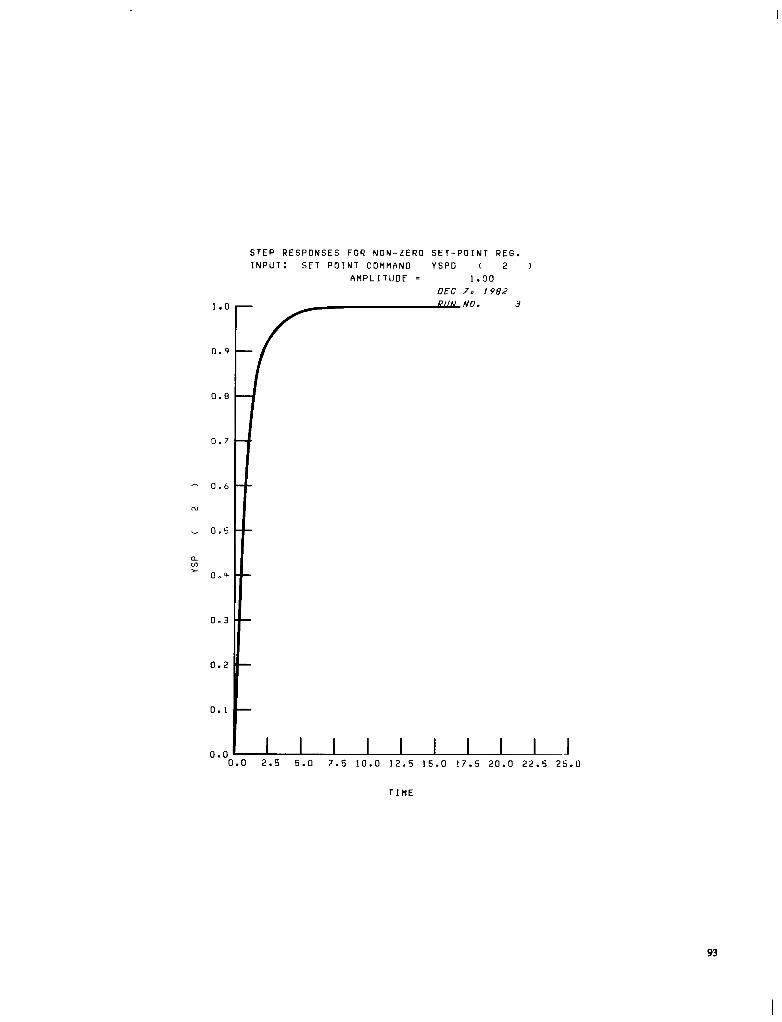
1.0

0.9

0.8

0.7

- 0.6

N

v 0.5

a m >

0 . Y

0.3

0 . 2

0.1

0.0 f

STEP RESPONSES FOR NON-ZERO S E T - P O I N T R E G . I N P U T : S E T P O I N T COMMANO YSPD ( 2 1

A M P L I T U D E = 1 .oo DEC 7. I982

1.0

93

As a final check, the control responses are examined for this design to see that required control excursions are within limits (*5.0). To do this, the user requests function 101, which allows changes to be made in reference values. In particular, the user changes elements of transient response selection matrices MSYSP and MSPU so as to request both the control responses and the output responses, thus displaying the interaction between output I and input 2 and vice-versa.

FUNCTION 0 TO COMPUTE FURTHER, ENTER NEXT FUNCTION NOS+(I3), ONE PER LINE TO TERMINATE ENTER 999(LAST ENTRY MUST BE A RETURN) 101 604

FUNCTION 101 CHANGES TO REFS

DISPLAY REFS BEFORE MAKING CHANGES? n ENTER CHANGES 'IO NAMELIST REFS [TSFTR, DT, FIY IIELF, ZERflAX! AMPSF', AMPSR,

MSPYSP, H S P U ~ MSROLY, MSROLX, )?ICCLY, MICtLX, MICCLU, HICOLY, MICOLX) AMPICXr IF, ISPACE, IOUT, IMEASt JINCI JIND, ITRMXt NCURVv LINLOli, M'SPYv

The program then displays the reference values and plots the requested transients.

SREFS 8REFS m s ~ r s ~ ~ 1 ~ 1 ~ = 0 ~ 1 ~ m s r r s r ~ 1 ~ 2 ~ = 1 ~ 0 ~ ~ ~ ~ r t ~ ~ l , l ~ = 1 , 1 , ~ ~ ~ ~ 1 ~ ~ 1 , 2 ~ = 1 ~ 1 L e n d

TSFTR= 1 .0 DT= 0.240 FI= 0.1.O.U-01 DELF= 0.1Ol3-01 ZERflAX= LOO.0 AMPSF = 5x I. 0 AMPSR= 581.0 AflPICX= JOY1.0 IF= 90 ISPACE= 1 IOUT= 1

JINC= 1 IMEAS= 1

JlNIl- 1 ITRMX= 100 NCI-IRV= 2 LINLqG-. 2

HSPYSP= C ' t 1, ?x07 1, 1 9 1 C MSPY.. 2 5 0 x 0

MSFU= 2x1. 3x0. 261.7 18x0 M S R O L Y = 2 J C $ O HSROLX= 2x1, 8x09 2 $ 1 , 238X:O MICCLY= 1, 2499x0 HICCLX= 2500x0 MICCLU= 250x0 HICOLY= I r 24991'0 MICOLX= 1 9 50x09 1. 2448*0 SEND ARE THERE ANYMORE CHANGES, Y OR N? m

FUNCTION 604 OBTAIN AND PLOT SELECTEn STEP RESPONSES FOR THE NON-ZERO SET POINT LINEAR REGULATOR

STATE TRANSITION MATRIX OF LINEAR REGULATOR FOR TIflE STEP 0.2400

1 2 3

1 0 . 9 0 8 9 0.1832 2 -0.5167 0.5573

0.7571?-02

3 -0.8230D-01 -0.2934 0.55S5D-01 0 .7855

94

I

F O R C E D R E S P O N S E M A T R I X O F L I N E A R R E G U L A T O R F O R T I M E S T E P 0 .2400

1 2 3

1 0,2315 2 -0.6794D-01 0.1856 3 -0.1475D-01 -0.3928D-01 0.2138

0.2420D-01 0.6469D-03 0.7636D-02

0.5

0.4

0.3

0.2.

- 0.1

m

v 0.0

D ul ). -. 1

-.2

- . 3

-.4-

- . 5 I

S T E P R E S P O N S E S F O R N O N - Z E R O S E T - P O I N T R E G . I N P U T : S E T P O I N T C O M M A N D Y S P D ( 1 )

A M P L I T U D E = I .oo DEC 7 9 I982 - RUN NO. 3

I-

T I M E

95

STEP RESPONSES FOR NON-ZERO SET-POINT REG.

0.0'

0.0:

0.0;

0.01

- 0.00

- - -.01

a m %

" 0 2

-.03

-.o+

-.05

INPUT: SET POINT COMMAND YSPD ( 2 1 AHPLITUDE = 1 .oo

DEC 7 s I982 RUN NO. 3

I I I I I I I I I I 5.0 7.5 10.0 12.5 15.0 17.5 20.0 22.5 25.0

T I H E

Note that there is some interaction between input 1 and output 2 but little between input 2 and output 1.

Finally, the four control responses are displayed. These responses confiim that design criterion 3 has been met. That is, both control signal absolute magnitudes remain less than 5 during a step response. The maximum excursion for u1 is + 1.07 and that for u2 is +2.98, both well below the design limits.

%

1.1

1 .o

0.9

0.8

- 0.7

d

0.6

3

0.5

0 . Y

0.3

0.2

0.1 0

STEP RESPONSES FOR NON-ZERO SET-POINT REG. I N P U T : S E T P O I N T COMMAND Y S P D ( 1 1

CtMPLITUDE = 1 .oo OEC 7 r I982 RUN NO. 3

97

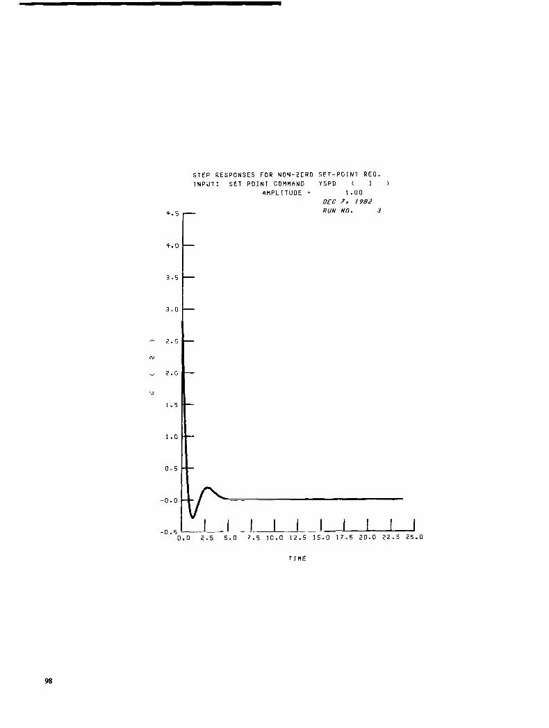
4. E

y., C

3.5

3.0

- 2.5

N

" z o o

3

1 . 5

1.0

0.5

-0.0

STEP RESPONSES FOR NON-ZERO SET-POINT REG- INPUT: SET POINT COt lHhND YSPD ( 1 )

4 H P L I T U D E = 1 . oo DEC 7 s I982 RUN NO. 3

98

1 .o

0 . 9

0.8

0.7

,-. 0 . 6

- - 0.5

3

0 . Y

0.3

0.2

0. I

STEP RESPONSES FOR NON-ZERO S E T - P O I N T REG. I N P U T : S E T P O I N T COMMAND Y S P O ( 2 )

A M P L I T U D E = 1 .oo OFC ? D I982 RUN NO. 3

2.5 5.0 7.5 10.0 12.5 15.0 17.5 20.0 22.5 25.0

99

-0 D

- 0 - 1

- 0 - s

-0 .1

- -0.;

> \ I

v -0.E

3

-0.9

-1.0

-1.1

- 1 . 2

3 -

\

+ -

I -

> -

7 -

l -

, -

I -

-

- 1 . 3 0.c

S T E P R E S P O N S E S F O R N O N - Z E R O S E T - P O I N T R E G . I N P U T : S E T P O I N T C O H H A N I : Y S P O ( 2 )

4 H P L I T U D E = 1 . oo OfC 7 0 I982 - RUN N O . 3

1 2.5 5.0 7.5 10.0 12.5 15.0 17.5 20.0 22.5 25.0

T I M E

100

After the responses are displayed, the user is again prompted for more requests, at which time the user terminates the program. The terminal session ends with the user requesting a printout of the output dataset (OUT=) that was generated during the present run for further off-line analysis if desired.

F U N C T I O N 0 T O C O M P U T E F U R T H E R 9 E N T E R N E X T F U N C T I O N N O S . ( I 3 ) , O N E P L R L I N E TO T E R M I N A T E E N T E R 9 9 9 C L A S T E N T R Y M U S T H E A R E T U R N ) 999

S T O R E T H E N 1 F O R T H I S R U N ? n C H C R W 4 0 0 T E R M I N A T E D : S T O F ' R E T U R N erint outaavPrtsr=edit C Z A H D O S O P R I N T P S N = 0 4 9 8 r 800 L I N E S o f f P007 L O G I C A L D I S C O N N E C T , L O G O N OR HANG UP

L @ G @ F F A T 1 4 1 4 0 @ N 0 7 / 0 7 / 8 1 - C'F'LI TlHE= 0 . 0 7 M l H U T E S .

101

Appendix D Terminal Output Options and Main PROCDEF

This appendix includes (1) a list of those items included in the “standard” terminal output, (2) a list of those items included in the “extended” terminal output, and (3) the PROCDEF that is used to set up the program before it is run.

Standard Terminal Output

The following data will be displayed in the user’s terminal if the user has requested the functions that generate these data:

(1) NAMELIST N1 (2) NAMELIST REFS (3) NAMELIST CONPAR (4) NAMELIST ESTPAR ( 5 ) NAMELIST MATDAT (6) Open- and closed-loop eigenvalues (7) Kalman filter eigenvalues (8) Transfer function numerator and denominator polynomial coefficients (9) Transfer function gains

(10) Maximum and average symmetry error for the SS and PP matrices (11) Positive-definiteness checks for the SS and PP matrices (12) Maximum element of and trace of the residual error matrix for the control and Kalman filter

(13) Lyapunov error check data consisting of Riccati equations

(a) Trace of residual (b) Normalized diagonal elements of error matrix (c) Trace of error (d) Trace of covariance (e) Ratio of trace of error to trace of covariance

(14) Normalizing factors (15) Error messages

Extended Terminal Output

The extended terminal output consists of all of the standard terminal output plus (1) Input matrices (2) All eigenvectors and mode shapes (3) The ATOT, CTOT, DTOT, KCTOT, and HTOT matrices (4) The SS matrix ( 5 ) The PP matrix (6) The KC matrix (7) The KE matrix (8) The KFF matrix (9) All covariance matrices

. (10) Controllability check matrix (1 1) Observability check matrix (through H) (12) Observability check matrix (through C) (13) Transfer function gains and zeroes (14) All state-transition matrices (15) All forced-response matrices (16) Symmetry error matrix for the control Riccati equation (17) Residual error matrix for the control Riccati equation (18) Symmetry error matrix for the Kalman filter Riccati equation

1 02

(19) Residual error matrix for the Kalman filter Riccati equation (20) Normalized system matrices: A, B, C, H, QQ, RRINV, D, DOUT, and CSP

PROCDEF AESRUN

The user invokes the following PROCDEF, AESRUN, before running the AESOP program. The purpose of the PROCDEF is to datadef all necessary libraries and required datasets. The PROCDEF requires one parameter (up to three characters), which is used to label all datasets that may be generated during the subsequent run of the AESOP program.

AESRUN 0000000 PROCDEF AESRUN AESRUN oooO100 PARAM $1 AESRUN oooO200 ERASE OUT$l AESRUN oooO300 DDEF FT06F001 ,VS,OUT$l ,DCB = (RECFM = V,LRECL = 132),RET = T

AESRUN oooO500 DDEF FTO8F001,.VS,CG$l; DISPLAY 'CG$1 IS DDEFD TO IO UNIT 8' AESRUN oooO600 DDEF FT09F001,VS,EG$l; DISPLAY 'EG$1 IS DDEFD TO IO UNIT 9' AESRUN oooO700 DDEF FTlOFOOl,VS,PFRUZ$l; DISPLAY 'PFRUZ$l IS DDEFD TO IO

AESRUN oooO800 DDEF FTllF001,VS,PFRUY$l; DISPLAY 'PFRUY$l IS DDEFD TO IO

AESRUN oooO900 DDEF FT12F001,VS,PFRWZ$l; DISPLAY 'PFRWZ$l IS DDEFD TO IO

AESRUN 0001000 DDEF FT13F001,VS,PFRWY$l; DISPLAY 'PFRWY$l IS DDEFD TO IO

AESRUN 0001100 DDEF FT14F001,VS,CFR$l; DISPLAY 'CFR$l IS DDEFD TO IO UNIT

AESRUN 0001200 DDEF FT15F001,VS,PP$l; DISPLAY 'PP$1 IS DDEFD TO IO UNIT 15' AESRUN 0001300 BBEF FT16F001,VS,SS$l; DISPLAY 'SS$l IS DDEFD TO IO UNIT 16' AESRUN 0001400 DDEF FT17F001,VS,FFG$l; DISPLAY 'FFG$l IS DDEFD TO IO UNIT

AESRUN 0001500 DDEF RUNl,VP,GRAPHICS, OPTION= JOBLIB; DISPLAY 'RUN1 IS

AESRUN 0001600 DDEF RUN2,VP,AESLIB,OPTION = JOBLIB: DISPLAY 'RUN2 IS

AESRUN 0001700 LOAD BLOCKA9; LOAD AESOP

AESRUN oooO400 DISPLAY 'OUT$l IS DDEFD TO THE HI-SPEED PRINTER'

UNIT 10'

UNIT 11 '

UNIT 12'

UNIT 13'

14'

17'

LIBRARY GRAPHICS'

LIBRARY AESLIB '

Eleven VS datasets that are to contain program input or output are datadeffed by this PROCDEF. Table I lists these datasets plus four others that might be datadeffed by the user during the course of running the program.

103

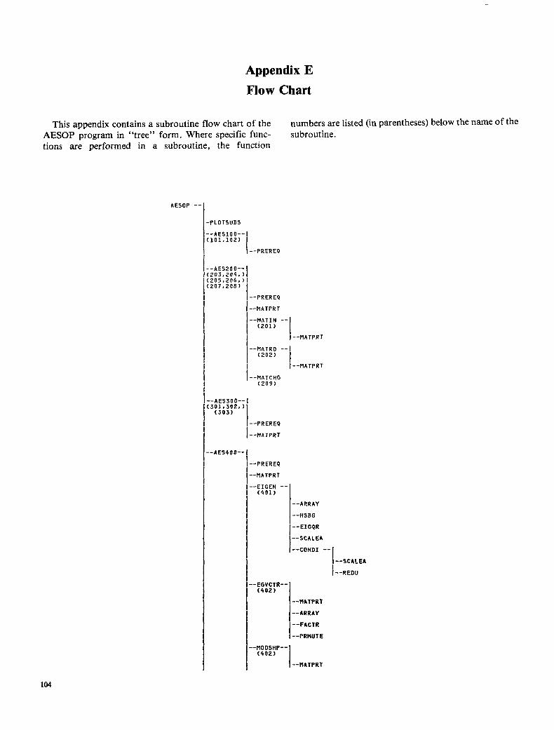
Appendix E Flow Chart

This appendix contains a subroutine flow chart of the numbers are listed (in parentheses) below the name of the AESOP program in "tree" form. Where specific func- subroutine. tions are performed in a subroutine, the function

AESOP --I -PLOTSUBS

- - A E s ~ o o - - I ( 1 0 1 , 1 0 2 ) I "PREREQ

I--AES3OO--i ( 3 0 1 . 3 0 2 , )

( 3 0 3 ) I "PREREQ

I --MATPRT

l A E s 4 0 0 - - '

1 --PREREQ

1 --MATPRT I I

"EIGEN -- ( 4 0 1 )

--ARRAY

I --HSBG

I -EIGQR

"SCALEA

--CONDI -- --SCALEA

I I--REDU

--EGVCTR--I I ( 4 0 2 ' j--RATPRT --ARRAY

--FACTR

--PRMUTE

! --MODSHP--

( 4 0 2 ) I I --RATPRT

104

I i --MXINV

/--PREREQ

--FRSPNS-- ( 5 0 1 , 5 0 4 . ) ( 5 0 7 , 5 1 0 . ) ( 5 1 3 , 5 1 5 , ) ( 5 1 7 , 5 1 9 . ) ( 5 2 1 . 5 2 3 )

"FRQP "/--FRpOLY

--BOLLIH--I

--DAVIS0

--DANSKY--

--POLMPY

I--BODE - - I ( 5 0 2 . 5 0 5 . ) 1 ( 5 0 8 . 5 1 1 , ) l ( 5 1 4 , 5 1 6 . ) ( 5 1 8 . 5 2 0 , ) ( 5 2 2 , 5 2 4 ) i

I-PLOTSUBS

-AES600--

"PREREQ

- -STP --I ( 6 0 1 , 6 0 4 )

I-PLOTSUBS

I --ICRSP --I ( 6 0 2 . 6 0 3 )

I

-AE5700--

--PREREQ

"MATPRT

I-- ZEROES-- ( 7 0 1 , 7 0 2 , ) ( 7 0 3 , 7 0 4 . )

( 7 0 5 )

--ARRAY

"HSBG

--EIGQR

--CONDI -- --SCALE4

--REDU

105

.-AES800-- 8 0 2 . 8 0 6 , . 808,810.: 814.816)

--GAIN : 7 0 1 , 7 0 2 , ) 7 0 3 . 7 0 4 , )

( 7 0 5 )

.-PREREQ

.-MATPRT

.-CONTRL-- ( 8 0 1 )

--MATPRT

--RICSS -- "MATPRT

--ARRAY

--EIXINV

--ORDER

I--E1GQR I - -SCALEA 1 --HSBG i - -EGCK --I j --PIODSHP-- I

I I I - -EGVCTR- -~

I

I --MATPRT

I "MATPRT

I - - A R R A Y

I "FACTR I --PRMUTE

--ARRAY

I "SCALEA I I --REDU

-EGVCTR-- (80/1)

"MATPRT

--ARRAY

"FACTR

I --PRMUTE

-MODSHP--

-RICCHK-- 8 0 7 , 8 1 5 )

--MATPRT

-ESTMAT-- (809 ) I

I --MATPRT

I--MATPRl

I "MXINV

106

--ORDER

--EIGQR

"SCALEA

--HSBG

--EGCK " 1 --MODSHP-- I I 1--MATPRT

--EGVCTR--

--MATPRT

--ARRAY

--FACTR

--PRMUTE

-COVAR -- ( 8 1 7 )

"MATPRT

-1YPCK - - I (818)

--ARRAY

--LAPNV --

i --MXINV ( 8 1 9 )

-AES900-- 9 0 1 . 9 0 2 . ) 9 0 3 . 9 0 4 ) I

--MATPRT

"ARRAY

"LAPNV --

"MXADO

"MXMLT

"MXTRA

--MXINV

--DSCA

"MXADO

"MXMLT

"MXTRA

--MXINV

--DSCA

--UZR901

--UZR902

--UZR903

"UZR904

107

Appendix F Prerequisite Table

This appendix contains the information used by the AESOP program to make prerequisite checks. These checks are performed before each AESOP iunction is to be executed to see that the necessary iunction or com- bination of functions has been performed prior to execution of the present function. Table XI1 lists this prerequisite check information in the following form: The specific prerequisite function or combinations of

functions are listed across the top, and each function whose prerequisites are to be checked is listed on the left. A checkmark appears in a row to indicate a prerequisite. Multiple checkmarks in a row indicate that the corresponding prerequisites are to be logically “ANDed.” For example, the logical prerequisite statement for function 303 is (201 OR 202) AND (205 OR 801) AND (206 OR 809).

108

TABLE XII. - PREREQUISITES FOR AESOP FUNCTIONS d

Function Prerequisite function c 404 501 - 201 3r 202

-

X X X X X X X X

X X X

X X

X

X

X

X

X

1 - 319 )r 209

- 206 or 809

X X

- 504

X X

- 507

X X

X

- 510

X X

X

X

- 513

X

- 515

X

- 519

X

- 523

- 205 or 801

X X X

- 207 or 801

- !08 )r 309

- 301

- 303 !05,

!06, 301, )r 309

101 ~ 102

201 202 203 2 04 205 206 207 208 209 210

301 302 303

401 402 403 404 405

501 502 503 504 505 506 507 508 509 510 511 512 513 514 515 516 517

519 518

520 521

x X

X X

X X

X X

X X

X

X

TABLE X I I . - Concluded, Function -""" Prerequisite function

None 201 205 206 207 208 301 ' 302 303 205, 401 ' 402 404 501 504 507 510 513 ' 515 517 519 521 523 801 803 809 817 819 or ZU9

""""" "-""""

or or or or or 202 801 809 801 809

206, 801, or 809

""""" ""-" ~ " - 522 523 524 525

601 602 603 604

701 7 02 703

7 05 704

801 802 803 804 805 806 807 808 809 810 811 812 813 814 815 816 81 7 818 819

I 901 820

X X

x x X X X X

X X

X

X

X

X

X

X

X X

X

X

X X

X X

1 i

X

X X

x

X

X X

X X

X

References

1. Lehtinen, B.; and Lorenzo, C.F.: Space ghuftle Active-Pogo- Suppressor Control Design Using Linear Quadratic Regulator Techniques. NASA TP-1217, 1979.

2. Lehtinen, B.; DeHoff, R.L.; and Hackney, R.D.: Multivariable Control Altitude Demonstration on the Fl00 Turbofan Engine. J. Guidance Control. vol. 4, no. 1, Jan.-Feb.

3. Geyser, L.C.; and Lehtinen, B.: Digital Program for Solving 1981, pp. 50-58.

4.

5 .

6.

7.

8.

9.

- the Linear Stochastic Optimal Contr.01 and Estimation Problem. NASA TN D-7820, 1975.

Lehtinen, B.; and Zeller, J.R.: Application of Quadratic Optimization to Supersonic Inlet Control. Automatica, vol. 8, no. 9, Sept. 1972, pp. 563-574.

Zeller, J.R.; et al.: Analytical and Experimental Performance of Optimal Controller Designs for a Supersonic Inlet. NASA TN

Kalman, R.E.; and Englar, T.S.: A User’s Manual for the Automatic Synthesis Program. NASA CR-475, 1966.

White, J.S.; and Lee, H.Q.: User’s Manual for the Variable Dimension Automatic Synthesis Program (VASP). NASA TM

Bryson, A.E., Jr.; and Hall, W.E., Jr.: Optimal Control and Filter Synthesis by Eigenvector Decomposition. (SUDAAR-436, Stanford Univ.; NASA Contract NAS2-5143.) NASA

Armstrong, E.S.: ORACLS - A System for Linear-Quadratic-

D-7188, 1973.

X-2417, 1971.

CR-152266, 1971.

Gaussian Control Law Design. NASA TP-I 106, 1978.

10. Konar, A.F.; et al.: Digital Flight Control System for Tactical Fighters, Vol. 2: Documentation of the Digital Control Analysis Software (DIGIKON). Honeywell-08001-VOL-2, Honeywell, Inc., June 1974, (AFFDL-TR-73-119-VOL-2, AD-A002327.)

11. Special Issue - Computer-Aided Design of Control Systems. IEEE Control Systems Magazine, vol. 2, no. 4, Dec. 1982.

12. Kwakernaak, H.; and Sivan, R.: Linear Optimal Control Systems. Wiley-Interscience, 1972.

13. Smith, P.G.: Numerical Solution of the Matrix Equation. AX+XAT+B=O. IEEE Trans. Autom. Control, vol. AC-16, no. 3, June 1971, pp. 278-279.

14. Smith, R.A.: Matrix Equation X A + B X = C . SIAM J. Appl. Math., vol. 16, no. 1, Jan. 1968, pp. 198-201.

15. Seidel, R.C.: Computer Programs for Calculation of Matrix Stability and Frequency Response from a State-Space System Description. NASA TM X-71581, 1974.

16. Davison, E.J.: A Computational Method for Finding the Zeroes of a Multivariable Linear Time Invariant System. Automatica, vol. 6, no. 3, May 1970, pp. 481-484.

17. Brockett, R.W.: Poles, Zeros, and Feedback; State Space Interpretation, IEEE Trans. Autom. Control, vol. 10, no. 2, Apr.

18. Kwatny, H.G.; and Fink, L.H.: Acoustics, Stability, and Compensation in Boiling Water Reactor Pressure Control Systems. IEEE Trans. Autom. Control, vol. AC-20, no. 6, Dec. 1975, pp. 727-739.

1965, pp. 129-135.

111

1 . Report No.

NASA TP-2221 4. Title and Subtitle

2. Government Accession No.

. .

AESOP: An Interactive Computer Program for the Desigr of Linear Quadratic Regulators and Kalman Fi l ters

Bruce Lehtinen and Lucille C. Geyser

3. Performing Organization Name and Address - .. . .~

National Aeronautics and Space Administration Lewis Research Center Cleveland, O h i o 44135

2. Sponsoring Agency Name and Address .. ~~

National Aeronautics and Space Administration Washington, D . C . 20546

3. Recipient's Catalog No.

5. Report Date ~~

January 1984 6. Performing Organization Code-

505-34-06 8. Performing Organization Report No.

"..

E- 1686 0. Work Unit No. '

~~~- .. ..

3. Type of Report and Period Covered ~ - .. . . " - - " . - .

Technical Paper - 4. Sponsoring Agency Code

" .

5. Supplementary Notes

i. Abstract

AESOP i s a computer program for use in designing feedback controls and s t a t e estimators for linear multivariable systems. AESOP i s meant t o be used in an interactive manner. Each design task t h a t the program performs i s assigned a "function" number. The user accesses these functions either (1) by inpcitting a l i s t of desired function numbers or ( 2 ) by inputting a single function number. I n the latter case the choice of the function will in general depend on the re- su l t s obtained by the previously executed function. The most important of the AESOP functions are those t h a t design linear quadratic regulators and Kalman f i l t e r s . The user interacts with the program when using these design functions by inputting design weighting parameters and by viewing graphic displays of designed system responses. Supporting functions are provided t h a t obtain system transient and frequency responses, transfer functions, and covariance matrices. The program can also compute open-loop system information such as s t ab i l i t y (eigenval ues) , eigenvectors , control 1 abi 1 i ty , and observabi 1 i t y . The program is wri t ten i n ANSI-66 Fortran for use on an IBM 3033 using TSS 370. Descrip- t ions of all subroutines and resul ts of two test cases are included in the appendixes.

. Key Words (Suggested by Author@)) 18. Distribution Statement

Feedback control; Computer-aided design; Multivariable control systems; Riccati

Unclassified - unlimited

regulator sponse; Kalman f i l t e r ; Linear quadratic equation; Linear systems; Frequency re-

STAR Category 63

Security Classif. (of this report) 20. Security Classif. (of this page) 21. No. of pages 22. Price'

' I 113 1 A06 Unclassified Unclassified

'For sale by the National Technical Information Service, Springfield, Virginia 22161

NASA-Langley , 1984

aesop: an interactive computer program for the … technical paper 2221 january 1984 aesop: an...

Documents