AEROSPACE APPLICATIONS OF CONTROLAEROSPACE APPLICATIONS OF CONTROL

CDS 101 SeminarCDS 101 SeminarOctober 18, 2002October 18, 2002

Scott A.Scott A. BortoffBortoff

Group Leader, Controls TechnologyGroup Leader, Controls Technology

United Technologies Research CenterUnited Technologies Research Center

2

• $26.6 billion (2000)• 153,800 employees• 3 business groups...

Carrier

Otis

Pratt & Whitney

Hamilton-Sundstrand

Sikorsky

International Fuel Cell

• Aerospace• Building Systems• Power Solutions

3

Seminar ObjectivesEmphasize the importance of modeling, feedback, uncertainty

• Provide three examples of modeling• Illustrate the relationship among modeling, uncertainty and feedback• Provide an example of dynamic analysis.

1. Jet Engine Control2. Electric Generator

Transmission Control3. Combustion analysis &

control

4

Jet Engine Control ObjectivesTrack commanded thrust while maintaining constraints

Thermal efficiency increases with burner temperature- nominal temperatures near melting point of parts- temperature overshoots rapidly degrade turbine life

Pressure and flow constraints on compressor stages, to avoid stall, surge, flutter.

Speed constraints on fan & spool (to avoid structural failure).Structural constraints on fan & spool speeds

But…

• Fan and compressor efficiency best near stall, surge, and flutter boundaries.

• Thermal efficiencies highest with increased burner temperatures.

• Structure designed to minimize weight.

5

JSF capable of vertical T/L

• 3DOF nozzle• Roll posts• Lift fan

Challenges:

• Split Thrust has 10x bandwidth• Precise modeling requirements• Multivariable, nonlinear

3 DOF Nozzle

Roll posts

Lift fan

F-135 Engine ControlVTOL requirement means demanding control problem

6

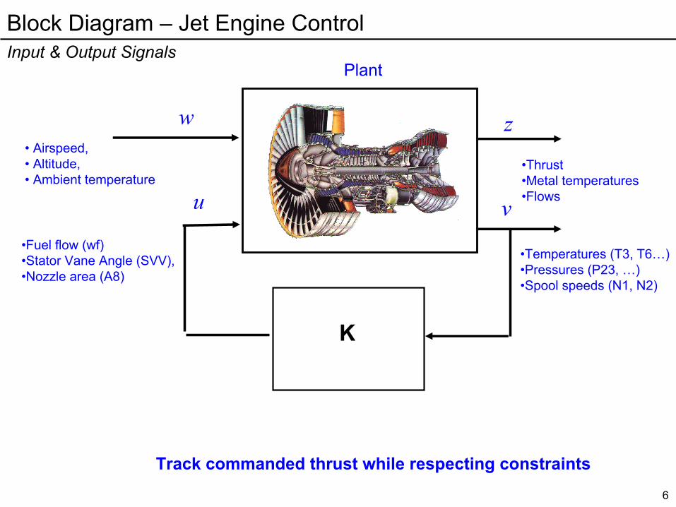
Block Diagram – Jet Engine ControlInput & Output Signals

•Temperatures (T3, T6…)•Pressures (P23, …)•Spool speeds (N1, N2)

Plant

v

zw

u

•Fuel flow (wf)•Stator Vane Angle (SVV),•Nozzle area (A8)

•Thrust•Metal temperatures•Flows

• Airspeed,• Altitude,• Ambient temperature

K

Track commanded thrust while respecting constraints

7

Jet Engine Dynamic ModelingNonlinear modeling

•Temperatures (T3, T6…)•Pressures (P23, …)•Spool speeds (N1, N2)

Nonlinear Plant Model

v

zw

u

•Fuel flow (wf)•Stator Vane Angle (SVV),•Nozzle area (A8)

•Thrust•Metal temperatures•Flows

• Airspeed,• Altitude,• Ambient Temperature

K

• Component Maps (fans, compressors)• Dynamic elements (control volumes, inertias)• Thermal Capacitances,

Corrected Airflow

Pre

ssur

e R

ise

Stall line

Constant N1

Steady state operating line

Nonlinear models embodied in code,

validated in engine or component tests.

8

Jet Engine Control-oriented modelF100 example

•Fan speed (N1) •Compressor speed (N2) •Compressor discharge pressure• Interturbine volume pressure• Augmentor pressure• Fan discharge temperature• Duct temperature• Compressor discharge temperature• Burner exit temperature 1 (fast)• Burner exit temperature 2 (slow)• Burner exit total temperature• Fan inlet temperature 1 (fast)• Fan inlet temperature 2 (slow)• Fan turbine exit temperature• Duct exit temperature 1• Duct exit temperature 2

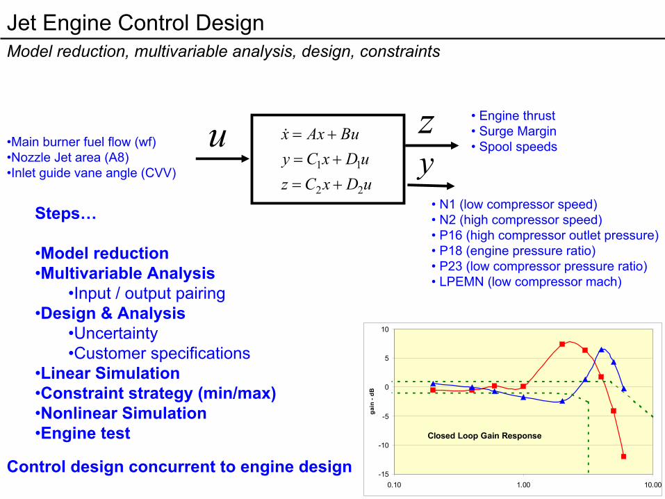
•Main burner fuel flow (wf)•Nozzle Jet area (A8)•Inlet guide vane angle (CVV)

• N1 (low compressor speed)• N2 (high compressor speed)• P16 (high compressor outlet pressure)• P18 (engine pressure ratio)• P23 (low compressor pressure ratio)• LPEMN (low compressor mach)

uDxCzuDxCy

BuAxx

22

11

+=+=

+= zu• Engine thrust• Surge Margin• Spool speeds

y

9

Jet Engine Control DesignModel reduction, multivariable analysis, design, constraints

Closed Loop Gain Response

-15

-10

-5

0

5

10

0.10 1.00 10.00

gain

- dB

Steps…

•Model reduction•Multivariable Analysis

•Input / output pairing•Design & Analysis

•Uncertainty •Customer specifications

•Linear Simulation•Constraint strategy (min/max)•Nonlinear Simulation•Engine test

• N1 (low compressor speed)• N2 (high compressor speed)• P16 (high compressor outlet pressure)• P18 (engine pressure ratio)• P23 (low compressor pressure ratio)• LPEMN (low compressor mach)

uDxCzuDxCy

BuAxx

22

11

+=+=

+= zu• Engine thrust• Surge Margin• Spool speeds

y•Main burner fuel flow (wf)•Nozzle Jet area (A8)•Inlet guide vane angle (CVV)

Control design concurrent to engine design

10

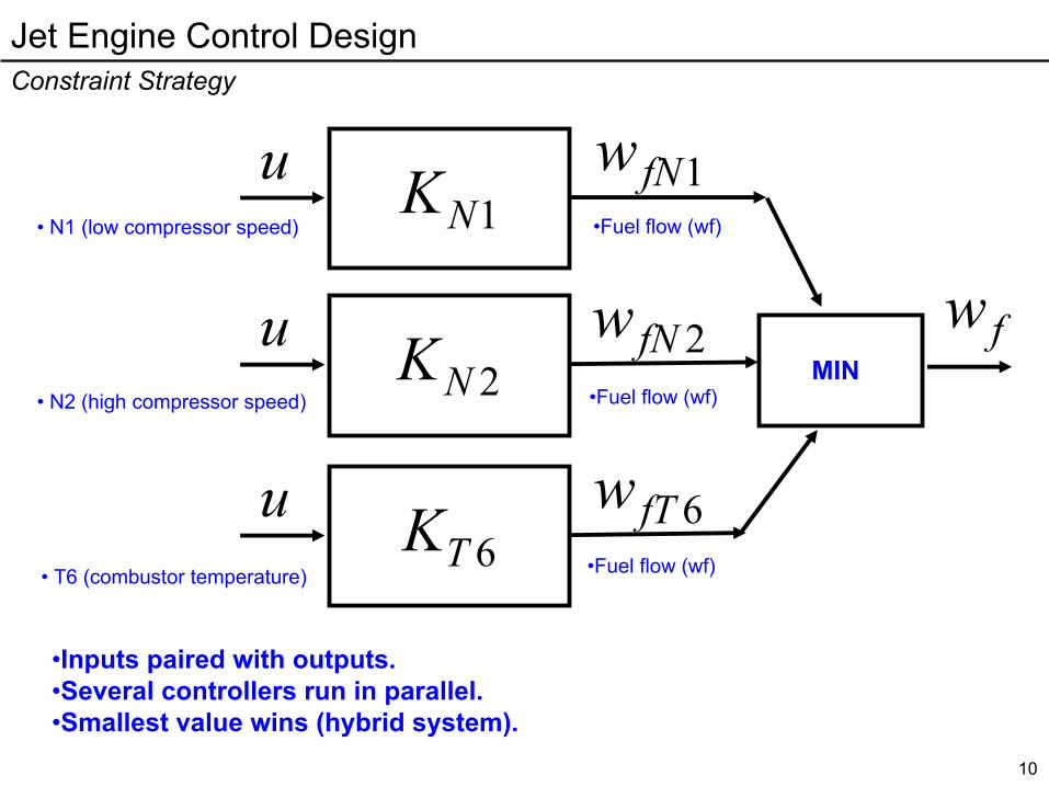
Jet Engine Control DesignConstraint Strategy

1fNwu1NK

• N1 (low compressor speed) •Fuel flow (wf)

2fNwu2NK

• N2 (high compressor speed) •Fuel flow (wf)

6fTwu6TK

• T6 (combustor temperature) •Fuel flow (wf)

MINfw

•Inputs paired with outputs.•Several controllers run in parallel.•Smallest value wins (hybrid system).

11

Can we close the loop on thrust ?Simplified Robustness Analysis

K Pve 1N1Nr

)()(

1 ωωjR

jE

N

CP+11

ω

Sensitivity function

)()(

1 ωωjR

jE

N

ω

MPCMMPC

RE

ˆ1)ˆ(

+−

=

K Pve 1Nthrustr Thrust

M

M̂

NPCNNPCˆ1

)ˆ(+

−

CPRE

+=

11

12

Example 2: Continuously Variable TransmissionsIntroduction

CVTs Used to couple variable speed spool to constant frequency generator.

Current designs use planetary gear with hydraulic actuation to “add” or “subtract” speed.

HS owns 92% of the world’s market in airborne electrical generation.

13

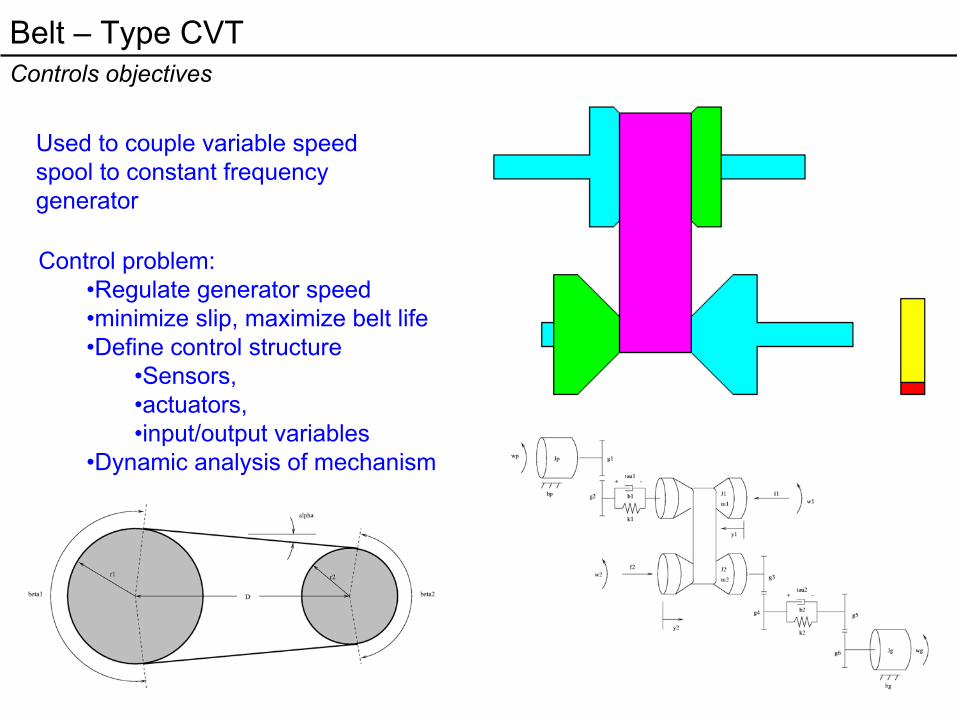
Belt – Type CVT Controls objectives

Used to couple variable speed spool to constant frequency generator

Control problem:•Regulate generator speed•minimize slip, maximize belt life•Define control structure

•Sensors, •actuators, •input/output variables

•Dynamic analysis of mechanism

14

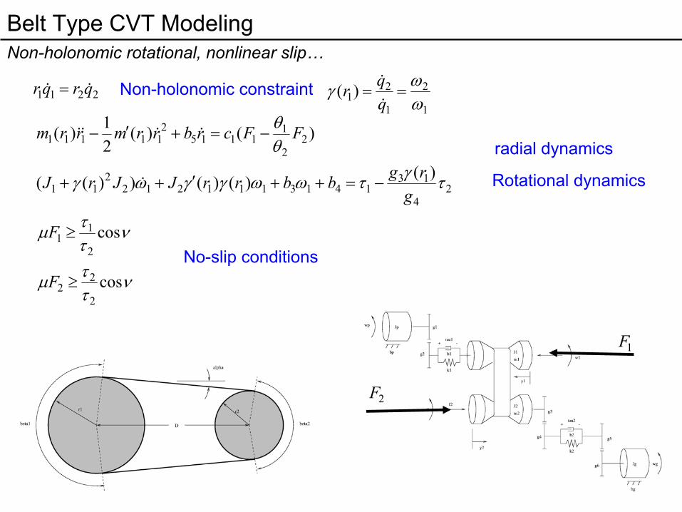
Belt Type CVT ModelingNon-holonomic rotational, nonlinear slip…

2211 qrqr = Non-holonomic constraint

24

131413111212

211

22

11115

211111

)()()())((

)()(21)(

τγτωωγγωγ

θθ

grgbbrrJJrJ

FFcrbrrmrrm

−=++′++

−=+′−

Rotational dynamics

1

2

1

21)(

ωωγ ==

qqr

radial dynamics

1F

2F

νττµ

νττµ

cos

cos

2

22

2

11

≥

≥

F

FNo-slip conditions

15

CVT Anti-Slip ControlModels enable dynamic analysis, trade studies, parameter selection

2

2

2

2

2

2

2

2

2

2

2

2

1

1

1

1

kJs

kbs

dkJs

kbs

kbs

L

L

++=

++

+=

τ

ττ

Lτ

νττµ

νττµ

cos

cos

2

22

2

11

≥

≥

F

F

Zero means overshoot

d2τ

Main result: Bandwidth of hydraulic actuation system (F1, F2) must exceed bandwidth of tau2 / taul to prevent slip.

16

CVT Speed ControlModels enable dynamic analysis, trade studies, parameter selection

Zero limits performance

gω2ω

•Generator speed can be regulated using engine spool, generator speeds as measurements.•Model uncertainty in spring / damper limits performance.•Higher performance achievable if w2 measured (robustness to uncertainty).

21 FF −)(1 sP

)(2 sω

)(2 sP)(sgω

1F

2F

reference

)(sK

referencereference

17

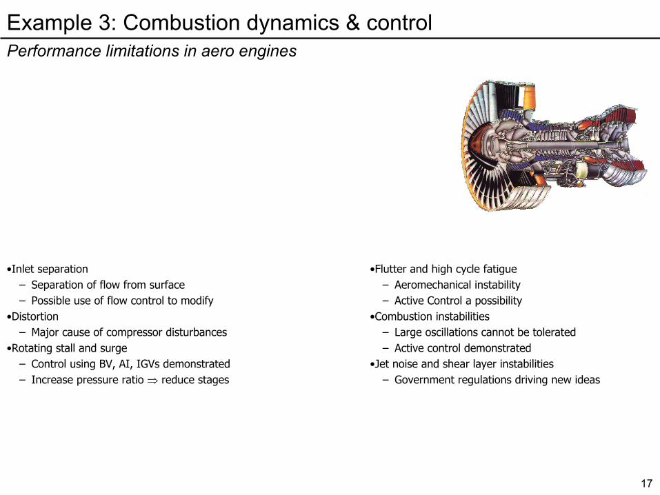
Example 3: Combustion dynamics & controlPerformance limitations in aero engines

•Inlet separation– Separation of flow from surface– Possible use of flow control to modify

•Distortion– Major cause of compressor disturbances

•Rotating stall and surge– Control using BV, AI, IGVs demonstrated– Increase pressure ratio ⇒ reduce stages

•Flutter and high cycle fatigue– Aeromechanical instability– Active Control a possibility

•Combustion instabilities– Large oscillations cannot be tolerated– Active control demonstrated

•Jet noise and shear layer instabilities– Government regulations driving new ideas

Inlet Buzz

Compressor

Stall, Surge &Flutter

Inlet Separation

Combustion Instab.

Shear Layer Instab.

Turbulence

Inlet Recovery

Distortion

Distortion Tolerance

Noise

Turbine Tip ClearanceBearing & Seal

Technology

18

Combustion Instabilities Will Occur

Equivalence Ratio

0

10

20

30

40

50

NO

x @

15

% O

2

Efficiency (%)

60

70

80

90

100

91

92

93

94

95

96

97

98

99

100Efficiency101

0.40 0.42 0.44 0.46 0.48 0.50 0.52 0.54 0.56 0.58 0.60

NOxLBO Combustion

Instability

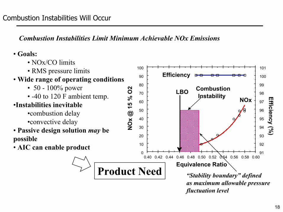
Combustion Instabilities Limit Minimum Achievable NOx Emissions

• Goals:• NOx/CO limits• RMS pressure limits

• Wide range of operating conditions• 50 - 100% power• -40 to 120 F ambient temp.

•Instabilities inevitable•combustion delay•convective delay

• Passive design solution may be possible• AIC can enable product

“Stability boundary” definedas maximum allowable pressurefluctuation level

Product Need

19

Combustors Experience Instabilities

Data obtained in single nozzle rig environment showing abrupt growth of oscillations as equivalence ratio is leaned out to obtain emissions benefit

20

Feedback Perspective on System Dynamics

Acoustic subsystem

Heat Release subsystem

Fluctuating heat release driven by unsteady velocity

Fluctuating pressure driven by unsteady heat release

•What is feedback? System coupling of a special type where inputs and outputs are dependent.

•Where does it occur? Most physically oscillatory (resonant) systems contain feedback - combustion dynamics is a prime example as shown. All control systems (sensor-actuator-controller or passive realization) contain explicit feedback loops.

•How is it used? To change dynamics and to cope with uncertainty.

•Why use it and when should it be applied? When dynamics are not favorable.

21

Stability analysis of combustion models using Nyquist criterion

noiseacoustics

combustion-F

)(22

2

tFtd

dtd

d=++ ηϖ

ηα

η

η

)()( τη −= ttd

dKtF

Acoustic mode driven by heat release

Pressure-sensitive heat release

-+

Bode plots for τ=0, 4ms, 5ms

Nyquist for τ=0 Nyquist for τ=4ms

-1.2 -1 -0.8 -0.6 -0.4 -0.2 0

-0.5

-0.4

-0.3

-0.2

-0.1

0

0.1

0.2

0.3

0.4

0.5

-1 -0.8 -0.6 -0.4 -0.2 0 0.2 0.4 0.6 0.8

-1

-0.8

-0.6

-0.4

-0.2

0

0.2

0.4

-1.4 -1.2 -1 -0.8 -0.6 -0.4 -0.2 0 0.2 0.4 0.6

-0.8

-0.6

-0.4

-0.2

0

0.2

0.4

0.6

0.8

100 120 140 160 180 200 220 240 260 280 3000

0.2

0.4

0.6

0.8

1

100 120 140 160 180 200 220 240 260 280 300

-800

-600

-400

-200

0

-1 inside => unstable

Nyquist for τ=5ms

22

0 200 400 600 800 10000

2

4

6

8

10

12

14

Am

plitu

de(p

si)

Uncontrolled, No CL Pilot11 ppm NOx, 37 ppm CO

Controlled8 ppm NOx, 17 ppm CO

experiment in UTRC 4MW Single Nozzle Rig demonstrates 6X reduction in pressure amplitude, decrease in NOX & CO emissions

Heated, highpressure air

Chokedventuri

Bypass legBurst disk

Main fuel Pilot fuel

CombustorPremixingfuel nozzle

Choked orificeplate

Gas samplingprobe (6)

Control theory provides methods for enforcing desirable behavior

Control: a fraction of main fuel modulated by a valve driven by phase-shifted signal from a pressure transducer

Example: Combustion Dynamics - Controlled and Uncontrolled

23

Data Analysis

Key parameters extracted from experiment (forced response tests) - trend in equivalence ratio (time delay) drives dynamical behavior

Calibration

•System level model captures experimental data quantitatively

Evaluation of Mitigation Strategies

•Evaluate passive design changes (resonators) for size, placement, prediction of performance

•Evaluate active control for actuation requirements (bandwidth) and prediction of performance

Combustion Dynamics & Control: Model Calibration and Use in Evaluation of System Modifications

0.45 0.5 0.55 0.6 0.65 0.70

0.5

1

1.5

2

2.5

3

3.5

4

4.5Amplitude of pressure oscillations

phibar

ampl

itude

(%

)

0.46 0.48 0.5 0.52 0.54 0.56 0.583.5

3.55

3.6

3.65

3.7

3.75

3.8

3.85

3.9

3.95

4x 10

-3 Variation of T ime Delay w ith Equivalence Ratio - DARPA

Mean Equivalence Ratio

Tim

e D

elay

(se

cond

s)

0 50 100 150 200 250 300 350 400 4500

0.005

0.01

0.015Bode plots P4_2p over Vact and fits with 8 poles, 8 zeros: magnitude

Mag

nitu

de

Hz

0 50 100 150 200 250 300 350 400 450-1000

-800

-600

-400

-200

0Bode plots P4_2p over Vact and fits with 8 poles, 8 zeros: phase

Phas

e

Files r60p14 and r60p29

Fuel/airpremixing

nozzlem n m t

m i

Side branchresonator

Orifice(to turbine)

Combustor

Coupled Resonator - Combustor System

Linear Acoustics

G(s)ddt

e s− τH(.)

Nddt

p

q

pressure

heat release rate

e s c−τ

Feedback control modulatingequivalence ratio

Analysis allows calibration of model from data to enable quantitative studies

24

0 50 100 150 200 250 300 350 400 450 5000

0.2

0.4

0.6

0.8

1

1.2

1.4

1.6

psi

Frequency, Hz

uncontrolledsingle nozzle controldual nozzle controltriple nozzle control

no control

single nozzle

dual nozzle

triple nozzledual nozzle

triple nozzle

Results of closed-loop experiments

Can harmonic balance explain the observed behavior?

Case study: sector combustor controlled with on/off valves

DSPACE-based controller

UTRC 8 MW three-nozzle sector rig controlled with on/off valves

Experimental setup

25

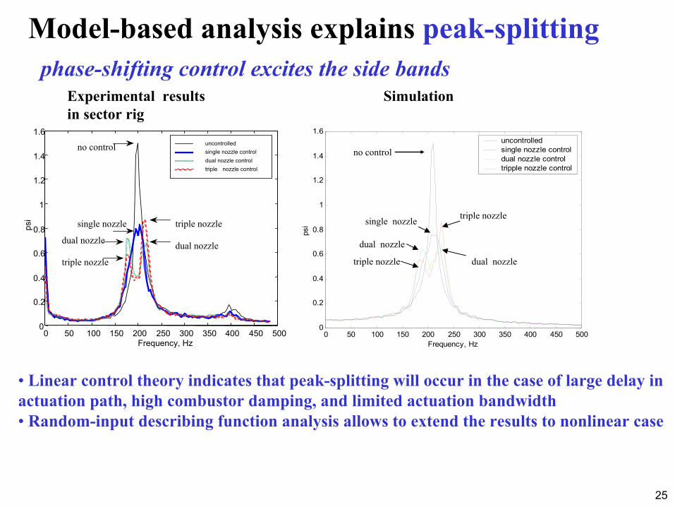
Model-based analysis explains peak-splittingphase-shifting control excites the side bands

0 50 100 150 200 250 300 350 400 450 5000

0.2

0.4

0.6

0.8

1

1.2

1.4

1.6

Frequency, Hz

psi

uncontrolled single nozzle control dual nozzle control tripple nozzle control

0 50 100 150 200 250 300 350 400 450 5000

0.2

0.4

0.6

0.8

1

1.2

1.4

1.6

psi

Frequency, Hz

uncontrolledsingle nozzle controldual nozzle controltriple nozzle control

no control

single nozzle

dual nozzle

triple nozzle

dual nozzle

triple nozzle

no control

Experimental results in sector rig

Simulation

triple nozzle

dual nozzle

single nozzle

dual nozzle

triple nozzle

• Linear control theory indicates that peak-splitting will occur in the case of large delay in actuation path, high combustor damping, and limited actuation bandwidth • Random-input describing function analysis allows to extend the results to nonlinear case

26

Fundamental limits can be studied in nonlinear models with noise using Random Input Describing Functions

0 100 200 300 400 500 600 700 800 900 1000-10

-8

-6

-4

-2

0

2

4

6

8 Sensitivity function

Log

Mag

-dB

Freq - Hz

+ +-

Conservation Principle: are under logarithm of sensitivity function is

preserved => peak splitting will occur

Pressure (j ω) Go(j ω)

Noise (j ω) 1+ N(A,σ)Gc(j ω) Go(j ω)

= Go(j ω) S(j ω), for

S(j ω)=1/(1+ N(A,σ) Gc(j ω) Go(j ω))

σ - STD of Gaussian component of valve command

A - amplitude of limit cycle in valve command

N(σ) - Random Input Describing Function

S(j ω) is a nonlinear analog of sensitivity function

=

Go(j ω)

Gc(j ω)

+-

PressureNoise

Valve command

Combustor

ControllerOn/off valve

b

-b

Peak splitting can occur in nonlinear systems, even limit cycling!

27

0 0.5 1 1.5 2 2.5 3 3.5 4 4.5 5-10

-5

0

5

10

15Second Order System - Low Damping

Time

Out

put

0 50 100 150 200 250 300-15

-10

-5

0

5

10

15

20

25

30

Frequency

Pow

er S

pect

rum

Mag

nitu

de (d

B)

•Evaluation of model sensitivities

•Development of experimental protocols and model calibration

•Evaluation of paths to mitigate undesirable behavior

Observed Unacceptable Time Response Behavior

System Level Model Showing Feedback Coupling

Effects of Parameter Variation on Stability Boundary

Model description capturing system

dynamics

Parametric analysis of system model

Enabling effective use of dynamic

model

Alter system dynamics to obtain acceptable behavior

0 1 2 3 4 5 6

x 10−3

0.5

0.6

0.7

0.8

0.9

1

1.1

1.2

1.3

tau

k

Stability boundary

Combustion Dynamics & Control:Role of Dynamic Analysis in Modeling/Design Cycle

Evaluation of Design Options

28

ConclusionsAerospace Applications of Control

• Control (feedback) analysis is useful beyond control system design.

• Modeling plays a central role.– Nominal plant– Uncertainty, disturbance signals,

• Modeling is done for a well-defined purpose.

29

BackupAerospace Applications of Control

30

Modeling and Analysis - Nyquist Criterion(2)

Nyquist criterion: translate closed loop properties into open loop properties

Observation: closed loop stability is equivalent to all poles of the closed loop transfer function lie in the open left half of the complex plane

Now use complex variable theory on the relevant transfer function -specifically use the so called principle of the argument

Principle of the argument: # of poles - # of zeros of a rational function inside Γ = winding number about the origin of the map G(Γ)

Graphically this is a mapping result (and a fancy way to count!)

GΓ

G(Γ)

31

Modeling and Analysis - Nyquist Criterion(3)

system shown is stable iff the zeros of 1+PC are in the open left half plane

But examine 1+PC: cp

cpcp

c

c

p

p

ddnndd

dn

dn

1PC1+

=+=+

closed loop poles

Now map the RHP under 1+PC and count encirclements of the origin

or

Map the RHP under PC and count encirclements of -1

cpcp

cp

nnddnn

PCPC

du

+=

+=

1

open loop poles

P

C

e

u

+-

ydcp

cp

ddnn

PCdu

== Open-loop TF

Closed-loop TF

32

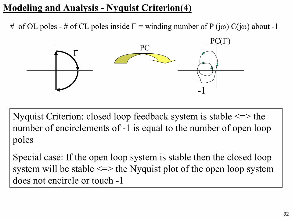
Modeling and Analysis - Nyquist Criterion(4)

PCΓ

PC(Γ)

-1

Nyquist Criterion: closed loop feedback system is stable <=> the number of encirclements of -1 is equal to the number of open loop poles

Special case: If the open loop system is stable then the closed loop system will be stable <=> the Nyquist plot of the open loop system does not encircle or touch -1

# of OL poles - # of CL poles inside Γ = winding number of P (jω) C(jω) about -1

33

Modeling and Analysis - Nyquist Example

Consider making the applied force a function of the velocity and choosing the function to

add dampingxkF 1−=

Approach I: Compute. Form the “closed loop system” and use computation to determine the closed loop eigenvalues (poles) and plot them as a function of the gain

Results for all gain (positive and negative) shown by the “root locus” plot

( ) 01

1

=+++−=++KxxkBxM

xkKxxBxM

01 >k

01 =k01 <k

x

BKM

F

34

Modeling and Analysis - Nyquist Example(2)

Approach II: Use Nyquist theorem. Form the block diagram of the “closed loop system” and use open loop properties to determine the closed loop stability as a function of the gain

F xKBsMs

s++2

1k−

Nyquist plot shows no encirclements of -1 point (for positive gain) so system is closed loop stable (but for increasing gain plot comes close and so there is decreasing margin) - for negative gain there are always two encirclements (unstable)

35

Modeling and Analysis - Nyquist Example(3)

Approach II: A bit of realism -suppose that the sensor for the rate (tachometer) has a small delay -what will be the effect on the stability of the closed loop system?

)()()()( 1 τ−−=++ txktKxtxBtxM

F xKBsMs

s++2

τsek −− 1

For small delays the Nyquist plot is unchanged but for large delays (or large frequencies) the plot is significantly different and the presence of a delay may alter stability - easily seen in the frequency domain!

Effect of delay: subtracts ωτ from the phase response of oscillator

36

Synthesis for Linear Systems - Nominal Stability

-1

Phase margin: angle that Nyquist curve can be rotated until instability

Gain margin: amplification that can be applied to Nyquistcurve until instability

•Nominal stability of the closed loop system can be easily ascertained using the Nyquist plot as shown,

•Typical values for gain margin are 6 dB and for phase margin 45-60 degrees P (jω) C(jω)

P

C

e

u

+-

yd

37

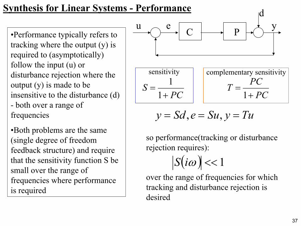
Synthesis for Linear Systems - Performance

•Performance typically refers to tracking where the output (y) is required to (asymptotically) follow the input (u) or disturbance rejection where the output (y) is made to be insensitive to the disturbance (d) - both over a range of frequencies

•Both problems are the same (single degree of freedom feedback structure) and require that the sensitivity function S be small over the range of frequencies where performance is required

eu yPC

d

TuySueSdy === ,,

so performance(tracking or disturbance rejection requires):

( ) 1<<ωiSover the range of frequencies for which tracking and disturbance rejection is desired

PCS

+=

11

sensitivity complementary sensitivity

PCPCT+

=1

38

Synthesis for Linear Systems - Robustness

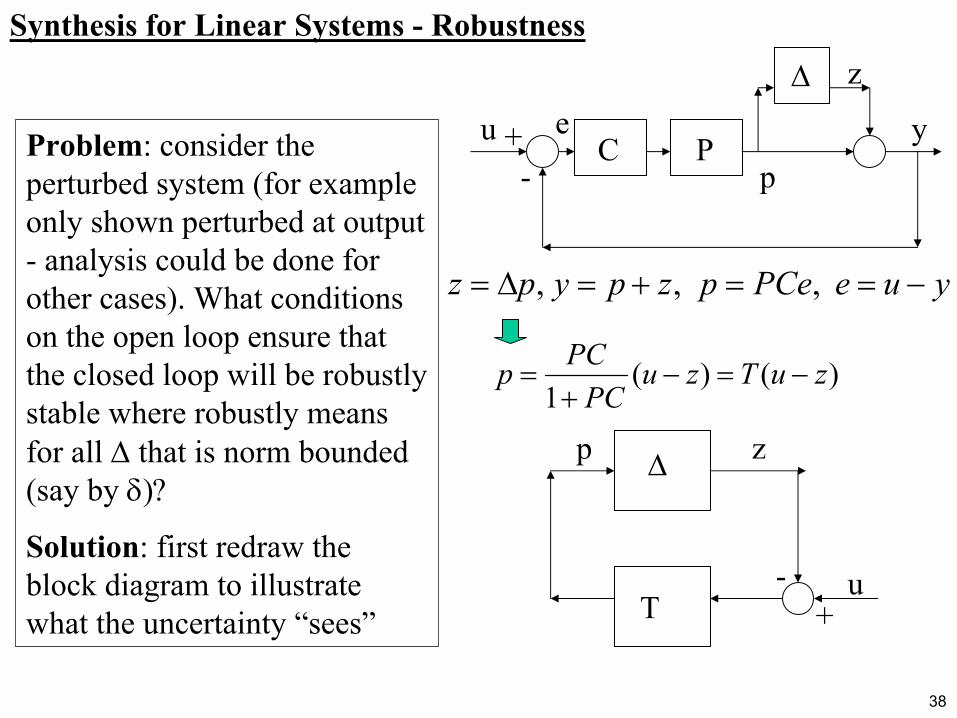
Problem: consider the perturbed system (for example only shown perturbed at output - analysis could be done for other cases). What conditions on the open loop ensure that the closed loop will be robustly stable where robustly means for all ∆ that is norm bounded (say by δ)?

Solution: first redraw the block diagram to illustrate what the uncertainty “sees”

eu y

z

pPC

∆

T

∆

yuePCepzpypz −==+=∆= , , ,

)()(1

zuTzuPC

PCp −=−+

=

p z

-+

-+

u

39

Synthesis for Linear Systems - Robustness(2)

Solution (continued):

•if the uncertainty is unknown (phase) then the T∆ loop is stable iff the “loop gain” is strictly < 1,

•recognize that the “loop gain” is the complementary sensitivity function and then this requires that the loop “roll off” at high frequencies

1ω

( )ωi∆

Typical shape for uncertainty (percentage of output) is small at low frequency and increasingly uncertain (especially phase) at high frequency

Robust stability then implies that the complementary sensitivity function “roll off” or to preserve robustness performance is sacrificed

( ) ( ) ωω

ω ∀∆

≤i

iT 1