aerosol analysis and forecast ecmwf integrated forecast

571

Aerosol analysis and forecast in theECMWF Integrated Forecast

System: Data assimilation

A. Benedetti1, J.-J. Morcrette1,O. Boucher2, A. Dethof1, R.J. Engelen1,

M. Fisher1, H. Flentjes3, N. Huneeus4,L. Jones1, J.W. Kaiser1, S. Kinne5,,

A. Mangold6, M. Razinger1,A.J. Simmons1, M. Suttie1, and the

GEMS-AER team

1European Centre for Medium-Range Weather Forecasts, Reading, UK2Met Office, Exeter, United Kingdom

3 Deutscher Wetterdienst (DWD), Offenbach, Germany4Laboratoire des Sciences du Climat et de l’Environnement, Gif-sur-Yvette, France

5 Max-Planck-Institut fur Mathematik, Bonn, Germany6 Royal Meteorological Institute of Belgium, Brussels, Belgium

Research Department

To be submitted to Journal of Geophysical Research

August 2008

Series: ECMWF Technical Memoranda

A full list of ECMWF Publications can be found on our web site under:http://www.ecmwf.int/publications/

Contact: [email protected]

c©Copyright 2008

European Centre for Medium-Range Weather ForecastsShinfield Park, Reading, RG2 9AX, England

Literary and scientific copyrights belong to ECMWF and are reserved in all countries. This publication is notto be reprinted or translated in whole or in part without the written permission of the Director. Appropriatenon-commercial use will normally be granted under the condition that reference is made to ECMWF.

The information within this publication is given in good faith and considered to be true, but ECMWF acceptsno liability for error, omission and for loss or damage arising from its use.

http://www.ecmwf.int/publications/

Aerosol analysis and forecast in the ECMWF Integrated Forecast System

Abstract

This study presents the new aerosol assimilation system developed at the European Centre forMedium–Range Weather Forecasts for the Global and regional Earth-system Monitoring usingSatellite and in-situ data (GEMS) project. The aerosol modelling and analysis system is fullyintegrated in the operational four–dimensional assimilation apparatus. Its purpose is to produceaerosol forecasts and reanalysis of aerosol fields using optical depth data from satellite sensors.This paper is the second of a series which describes the GEMS aerosol effort and focuses onthe theoretical architecture and practical implementation of the aerosol assimilation system. Italso provides a discussion of the background errors and observations errors for the aerosol fields,and presents a subset of results from the two–year reanalysis which has been run for 2003 and2004 using data from the Moderate Resolution Imaging Spectroradiometer on the Aqua and Terrasatellites. Independent datasets are used to show that, despite some compromises that have beenmade for feasibility reasons in regards to the choice of control variable and error characteristics,the analysis is very skillful in drawing to the observations and in improving the forecasts of aerosoloptical depth.

1. Introduction

Environmental monitoring is a fundamental activity in current times of rapid transformations of the natural en-vironment due to human activity. In particular, monitoring of greenhouse gases, reactive gases and atmosphericparticulate plays an important role due to the open–ended debate about climate change and its long–term im-plications (Bellouin et al. 2008). Issues raised by the proven links between some atmospheric constituents,such as ozone and particulate, and human health have also raised the level of attention toward these activities(Thompson et al. 2006; Lewtas 2007).

One of the fore-front projects dedicated to this goal is the Global and regional Earth-system (Atmosphere)Monitoring using Satellite and in-situ data (GEMS) project, which counts thirty-two European partners withexpertise in various aspects of atmospheric composition monitoring. GEMS is part of the Global Monitoringfor Environment and Security (GMES) initiative and was established under European Commission funding in2005 to create an assimilation and forecasting system for monitoring aerosols, greenhouse gases and reactivegases, at global and regional scales, through exploitation of satellite and in–situ data (Hollingsworth et al.2008). An important component of GEMS is also monitoring of regional air quality at the European scalewhich is performed with an ensemble of models from the participating institutes. Boundary conditions for thehigh–resolution models are provided by the global model.

The forecast and analysis systems which include atmospheric constituents have been developed. The basis forthese systems is the operational ECMWF Integrated Forecasting System (IFS1) and the incremental 4D-Varsystem, extended to include new prognostic variables for the atmospheric tracers (i.e. gases and aerosols). Acoupled chemical transport model is also part of the GEMS system and provides tendencies for the chemically–active species which are present in the model. In this paper, we will focus on the development and the per-formance of the aerosol analysis system. Companion papers by Morcrette et al. (2008) and by Mangold et al.(2008) discuss in details the aerosol model and the validation of the forecast/analysis results respectively.

Modelling and prediction of aerosols is associated with a large degree of uncertainty due to uncertainties in theemissions, transport and nonlinear physical processes involving aerosols (for example, radiative effects, cloudand rain formation, etc.). Ground–based observing networks have been crucial in improving our knowledge

1The documentation for the ECMWF Integrated Forecasting System is available online at www.ecmwf.int/research/ifsdocs/.

Technical Memorandum No. 571 1


of this atmospheric component, complemented in more recent years by satellite sensors which offer a moreglobal view of the aerosol distribution. Harmonization of models and data is, however, required in order totackle the model deficiencies and obtain a more accurate representation of aerosols and their interaction withthe atmospheric system as a whole.

The current attempt at variational data assimilation of satellite aerosol data into a Numerical Weather Prediction(NWP) model for reanalyses and forecasts is an unprecedented effort. Previous applications in this relativelyyoung field, aimed at assimilating aerosol in global models use the Optimal Interpolation approach with focuson regional studies (Collins et al. 2001; Rasch et al. 2001). A global assimilation OI system is described inGeneroso et al. (2007) and used to better constrain the Arctic aerosol burden. Weaver et al. (2007) describe anoff–line retrieval/assimilation system for the Goddard Chemistry and Aerosol Radiation Transport (GOCART)model using Moderate Resolution Imaging Spectroradiometer (MODIS) radiances based on the Kalman filterapproach. Successful 4D–Var aerosol assimilation has been implemented in a chemical transport model byFonteyn et al. (2000) and Errera and Fonteyn (2001). More recently, Zhang et al. (2008) described the firstattempt at building a 3D–Var system for operational aerosol assimilation using the Naval Research Laboratory(NRL) model, while Niu et al. (2008) introduced a novel data assimilation system for dust aerosols in theChinese Unified Atmospheric Chemistry Environment- Dust (CUACE/Dust) forecast system.

The scheme presented in this paper represents the European effort at building a pre–operational system forroutine aerosol assimilation and forecasting at global level. The aerosol assimilation is fully integrated as anoption within the general 4D–Var system employed operationally at ECMWF, and the aerosol model whichunderlies the assimilation is likewise integrated in the forecasting model. All aerosol species are model prog-nostic variables, advected by the semi-lagrangian scheme, consistently with other dynamical fields, and treatedas tracers in the vertical diffusion and convection schemes. They are also subject to aerosol–specific physicalprocesses such as sedimentation and wet/dry deposition. In the current model version, species included are seasalt, desert dust, black carbon, organic matter and sulphate. The emission sources for the various aerosol speciesare defined either using established emission inventories or through model–dependent parameterizations. Theobservational operator for aerosol optical depth uses the mass mixing ratios and pre-computed optical proper-ties according to the aerosol species at the specific wavelength. The control variable is the total aerosol mixingratio defined as the sum of the single contributing species. Background error statistics for this variable are com-puted with the NMC method and the background error covariance matrix is constructed using the “wavelet-Jb”approach. Errors for observations over ocean are defined using a parameterization which is function of theviewing geometry through a dependence on the scattering angle, while for observations over land an ad hocpercentage error is used. These errors are inflated with respect to the MODIS product specifications to accountfor representativeness errors deriving from the forward model and the observation processing.

The aerosol assimilation system has been recently completed and is currently being used to produce a two–year analysis for 2003–2004. Observations assimilated are the aerosol optical depths (AOD) retrieved from theMODIS instruments on board the Terra and Aqua satellites. The building blocks of the system are described insection 2. Section 3 presents the observations used in the reanalysis along with a discussion of biases and rep-resentativeness errors. The experimental set–up is also included in this section. Results for 2003 are examinedin section 5 with focus on the month of May 2003. A validation of these results using independent observa-tions from the AErosol RObotic NETwork (AERONET) is also presented. It is demonstrated that the GEMSaerosol assimilation system has good potential to provide high–quality analysis and forecasts of atmosphericparticulate.

2 Technical Memorandum No. 571


2. Technical description of the aerosol assimilation system

a. The aerosol model

The implementation of an aerosol module in the ECMWF model has involved the introduction of new prog-nostic variables (i.e. aerosol mass mixing ratios) and the definition of aerosol–specific physical parameteri-sations (Morcrette et al. 2006). The physical package for aerosols was partially taken from the Laboratoired’Optique Atmospherique (LOA) Laboratoire de Meteorologie Dynamique (LMD) model (Boucher et al. 2002;Reddy et al. 2005). It includes sources for sea salt and desert dust and a representation of sedimentation, andwet and dry deposition processes. The sedimentation scheme has been modified following recent developmentsby Tompkins (2005) while the wet and dry deposition schemes were adapted directly from the LMD model. Allaerosol species are treated as tracers in the IFS vertical diffusion and convection schemes and are advected bythe semi-Lagrangian scheme, consistently with all other dynamical fields and tracers. Five types of troposphericaerosols are included: sea salt, desert dust, organic matter, black carbon and sulphate aerosols. Stratosphericaerosols are not included in the current assimilation configuration.

Aerosols of natural origin are represented via a three-bin representation. Bin limits for sea salt are set at 0.03,0.5, 5 and 20 µm and for desert dust at 0.03, 0.55 0.9 and 20 µm. This ensures that approximately 10, 20 and70 % of the total mass is respectively included in the three bins. For organic matter and black carbon both thehydrophobic and the hydrophilic component are modelled. Sulphates are represented as one variable with noexplicit chemistry.

State-of-the-art emission sources have been implemented (Morcrette et al. (2006, 2008)). For anthropogenicaerosol, the sources come from available emission inventories (GFED, Global Fire Emission Database; SPEW,Speciated Particulate Emission Wizard; EDGAR, Emission Database for Global Atmospheric Research). Fornatural aerosol, the sources are instead related to model parameters (i.e. 10-m wind for sea salt, soil moistureand wind for desert dust, among others). The aerosol model provides the background information to feed intothe variational assimilation system described below.

b. The ECMWF 4D–Var

The variational method is a well–established approach to combine model background information and obser-vations to obtain the “best” forecast possible by adjusting the initial conditions. This approach is widely usedin many NWPs centres. The method is based on minimization of a cost function which measures the distancebetween observations and their model equivalent, subject to a background constraint usually provided by themodel itself. Optimization of this cost function is performed with respect to selected control variables (e.g. theinitial conditions). Adjustments to these control variables allow for the updated model trajectory to match theobservations more closely. Assuming the update to the initial condition (also known as the increment) is small,an incremental formulation can be adopted to ensure a good compromise between operational feasibility andphysical consistency in the analysis (Courtier et al. 1994). The cost function in the incremental approach canbe written as:

J(δx0) =12

δxT0 B−1δx0 +

12

n

∑i=0

(

H ′iδxi −di

)TR−1

i

(

H ′iδxi −di

)

+ Jc(δx0), (1)

where δxi = xi −xbi is the analysis increment and represents the departure of the model state (x) with respect to

the background (xb) at any time ti. H ′ is the linearized observation operator and di = yoi −Hi(xb

i) is the departureof the model background equivalent from the observation (yo

i ). The matrix Ri is the observation error covariancematrix, which comprise both pure observation errors (instrumental, calibration, retrieval) and representativeness



errors due to forward model assumptions and to the interpolations needed to go from model to observationspace. B represents the background error covariance matrix, formulated according to the “wavelet–Jb” methodof Fisher (2003; 2004). The aerosol–specific background error covariance matrix is discussed briefly in section2c and more extensively in Benedetti and Fisher (2007). The R and B matrices represent respectively therelative weight assigned to observations and background fields in the analysis. The background at t = 0, xb

0, isobtained from a short-range forecast valid at the initial time of the assimilation period. A penalty cost function,Jc(δx0), is used to impose all other physical constraints on the solution.

The flow of the 4D–Var minimization is as follows. A nonlinear integration provides the linearization state(trajectory) in the vicinity of which the model is linearized. The departures are computed during the nonlinearintegration at high resolution and then interpolated to the lower resolution. The gradient of the cost functionrequired in the minimization is computed using the adjoint model.

The minimization is solved using an iterative algorithm, based on the Lanczos conjugate gradient algorithmwith appropriate pre-conditioning. In order to reduce the computational costs and strong non-linearities in theoperational 4D–Var system, the perturbations δxi are computed with a tangent-linear model using simplifiedphysics (Tompkins and Janiskova 2004; Lopez and Moreau 2005) at a lower resolution than the trajectory.

After the minimization, the trajectory and the departures are recomputed and a second minimization at a higherhorizontal resolution is run. For the analysis a resolution of T159 (corresponding to ∼ 120 km) is used in thenonlinear trajectory and the forecast, while the two minimizations are run at T95 (∼ 215 km) and T159. Anaverage of 50–70 iterations are required to reach a satisfactory convergence of the minimization. Convergencecriteria and a detailed description of the incremental 4D–Var can be found in Fisher (1998) and Tremolet (2005).

The current assimilation window is 12 hours. MODIS observations of aerosol optical depth are ingested overthe window and sub–divided into time slots of half hour, together with all other meteorological data. A thinningis applied to better match the spatial resolution of the observations to that of the analysis.

The model fields, including aerosol mass mixing ratios, required by the operators are interpolated at the ob-servation locations and the model equivalent of the observations is computed using the specific observationoperator. The operator for AOD is described in section 2d.

c. The background error covariance matrix for aerosols

The aerosol B matrix used for the GEMS aerosol reanalysis was derived using the Parrish and Derber method(also known as NMC method, Parrish and Derber (1992)) as detailed in Benedetti and Fisher (2007). Thedifference with respect to the results presented in that paper lies in the use of updated error statistics derivedfrom forecast differences computed with the current aerosol model described in section 2a. The method is thefollowing: six months of 2-day forecasts at T159 are run and the differences between the 48-h and the 24-hforecasts are used as statistics for the estimate of the background errors. These are in turn used to construct aB matrix using the wavelet technique devised by Fisher (2003, 2006). In section 4a the sets of statistics fromthe run of Benedetti and Fisher (2007) and the current configuration are presented. Their impact on the aerosolanalysis is also discussed.

Benedetti and Fisher (2007) showed that the NMC method leads to a satisfactory background error covariancematrix without the need to prescribe the vertical and horizontal correlation lengths. The NMC method appliedto the definition of background error statistics for aerosol has also been revisited and compared with othermethods by Kahnert (2008) who concluded that it is the most appropriate for assimilation over the time windowstypically used in NWP applications (6-12 hours).



d. Observation operator

The observation operator for aerosol optical depth is based on pre-computed optical properties (mass extinc-tion coefficient, αe, single scattering albedo, ω , and asymmetry parameter, g) for the relevant aerosol speciesincluded in the model. The aerosols are assumed to be externally mixed, i.e. the individual species are assumedto co-exist in the volume of air considered and to retain their individual optical and chemical characteristics.These characteristics are computed at the MODIS wavelengths using Mie theory, e.g. particles are assumedto be spherical in shape, and integrated over the physical size range using a prescribed lognormal distribution(Reddy et al. 2005). Optical properties of hygroscopic aerosols such as sulphate, hydrophilic organic matter andsea salt, are parameterized as a function of relative humidity (RH). Table 1 summarizes the optical propertiesat 550 nm and 50% RH.

Table 1: Optical properties at 550 nm and 50% Relative Humidity.

Aerosol type αe (m2g−1) ω g

Sulphate 6.609 1.000 0.673Black Carbon 9.412 0.206 0.335Organic matter 5.502 0.982 0.655

Dust(0.03-0.55 µm) 2.6321 0.9896 0.7300(0.55-0.9 µm) 0.8679 0.9672 0.5912(0.9-20.0 µm) 0.4274 0.9441 0.7788

Sea salt(0.03-0.5 µm) 3.0471 0.9996 0.7394(0.5-5.0 µm) 0.3279 0.9961 0.7703

(5.0-20.0 µm) 0.0924 0.9916 0.8224

For the calculation of the model equivalent optical depth, the relative humidity is computed from model tem-perature, pressure and specific humidity. The appropriate mass extinction coefficients are then retrieved fromthe look–up table for the wavelength of interest (here, 550 nm), multiplied by the aerosol mass which has beenpreviously interpolated at the observation locations, and then integrated vertically. The total optical depth is thesum of the single–species optical depths as given by

τλ =N

∑i=1

∫ 0

psur f

αei(λ ,RH(p))ri(p)d pg

, (2)

where N is the total number of aerosol species, r is the mass mixing ratio, d p is the pressure of the model layerand g is the constant of gravity. psur f represents the surface pressure.

e. Total aerosol mixing ratio as control variable

The aerosol model comprises a mixed bin and bulk representation of the aerosol species. This was deemedto be a necessary compromise between a full–blown bin representation of all species which would have intro-duced many more tracers in the IFS, and a modal representation of the aerosols which would have possiblyover–simplified the aerosol model. However, the eleven additional tracers that are currently used in the forwardmodel, can constitute a heavy burden for the analysis if they are all included in the control vector. The reasonfor this is three–fold: (i) background error statistics would have to be generated for all species separately, (ii)the control vector would be much larger in size which would, in turn, increase the cost of the iterative minimiza-



tion, and most importantly (iii) the aerosol analysis would be severely under–constrained as one observation oftotal aerosol optical depth would be used to constrain eleven profiles of aerosol species. As a way to alleviatethese problems, the total aerosol mixing ratio, defined as the sum of the eleven aerosol species, is used insteadas control variable. The increments in the total mixing ratio deriving from the assimilation of MODIS opticaldepths have to be re–distributed into the mixing ratios of the single species. Even with this expedient, the prob-lem remains under–constrained with respect to the observations, and the redistribution of the increments reliesheavily on the background. However, the size of the control vector is more manageable. Some assumptions areneeded in order to implement this control variable correctly:

1. the sum of the single species have to be equal to the total mixing ratio at all times and for all locations,i.e. the aerosol mass needs to be conserved over the 12–hour assimilation window;

2. the relative contribution of a single species/bin to the total mixing ratio has to be kept constant over theassimilation window.

Assumption (1) implies that processes which do not conserve the aerosol mass, such as deposition and sedi-mentation, should not be activated during the trajectory run. Assumption (2) follows from (1), and effectivelyimplies that perturbations from species with higher specific density contribute more to the perturbation in totalmixing ratio even if their contribution to the optical thickness at a given wavelength might be smaller thanthat of species with lower specific density. In practice these assumptions are relaxed and the trajectory run isperformed with all aerosol processes switched on. This still provides a meaningful analysis since most of thedominant physical processes happen over time–scales longer than 12 hours. For example, the typical residencetime for the largest bin of desert dust and sea salt is approximately one day, whereas anthropogenic specieshave a typical residence time of a week.

The way this control variable works in practice is the following. In the nonlinear trajectory run the total aerosolmixing ratio is computed by summing all other species/bins, i.e. rT = ∑N

i=1 ri, where r is the mixing ratio, andthe subscript T indicates the total mixing ratio. All aerosol variables, including the total aerosol mixing ratio,are subject to advection, vertical diffusion and convection. The mixing ratios of the individual species are usedto compute the total optical depth using the tabulated optical properties as outlined in section 2d. The tangentlinear run is then started with zero perturbations for the single species to compute the perturbation in opticaldepth. The latter is passed to the adjoint routine to compute the gradient with respect to the individual species.The gradient with respect to the total mixing ratio is obtained as

r′

T =N

∑i=1

fir′

i (3)

where r′

is gradient of the mixing ratio and fi =( ri

rT

)

is the fractional contribution of the single species to thetotal mass. The gradient with respect to the total mixing ratio is then used in the minimization and the resultingincrement in rT is used in the following iteration of the tangent linear run to compute updated perturbations onthe individual species/bin mixing ratios as follows

r′

i = fir′

T . (4)

These, in turn, are used to compute perturbations in optical depth to be fed to the adjoint, and so on until theconvergence criteria is met. To avoid the analyzed total aerosol mixing ratio becoming negative as a result ofadding a negative increment, the total aerosol mixing ratio is screened for values less than zero and reset to zerowhen those happen.



3. Data description and experimental setup

a. MODIS aerosol retrievals

Of the available satellite data sources for aerosol optical depth data, the MODIS instrument on board of Terraand Aqua was selected for its accuracy and reliability. The availability of data in near real–time was a furtherfactor. These are important aspects in view of an operational application. The retrievals of aerosol optical depthfrom MODIS are described in Remer et al. (2005). Two separate retrievals with different accuracies are appliedover land and ocean. The retrievals over land suffers from higher uncertainties due to the impact of the surfacereflectance, notoriously harder to model over land than ocean. Over highly reflective surfaces such as desertsand snow-covered areas, there is no sufficient contrast to discern the signal coming from the aerosols over thatcoming from the surface. For this reason, the land retrieval is only possible over “dark” surfaces. Several otherfactors affect the accuracy of the retrievals both over land and ocean: cloud contamination, assumptions aboutthe aerosol types and size distribution, near–surface wind speed, radiative transfer biases, and instrumentaluncertainties. These factors are reviewed in detail in Zhang and Reid (2006).

For our purposes the most recent MODIS release (collection 5) was used since it has been proven to be moreaccurate, particularly over land. MODIS retrieved optical depths are provided at different wavelengths Theseare 470 nm, 550 nm, 660 nm, 870 nm, 1240 nm, 1630 nm and 2130 nm. However, as a first step, only theoptical depth at 550 nm is assimilated in the analysis. In what follows it is understood that aerosol optical depthrefers to the aerosol optical depth at a wavelength of 550 nm, unless otherwise stated.

The original data have a resolution of 10x10 km. Since the analysis is run at T159 which is approximately120x120 km, the MODIS optical depths are thinned to this coarser resolution. Observations are taken at theoriginal location and model aerosol fields are interpolated to this location before applying the observationoperator described in section 2d.

b. Discussion of observations and model biases

Observations and model biases are very important to characterize for a successful analysis as the analysis itselfdoes not remove biases, but only aims at minimizing the error between model and observations in a least squaresense. Zhang and Reid (2006) propose a method to remove biases from the MODIS ocean aerosol productbefore assimilation in the NRL system through quality assurance procedures and selective data screening.They indicate that the reduction in error between the corrected MODIS and the AERONET verifying data canbe 10-20%, mainly due to the elimination of the cloud–contaminated retrievals.

While recognizing the validity of this effort we did not apply a similar rigorous procedure to the MODISdata. Our approach was instead to devise a correction dependent on the model optical depth as described inBenedetti and Janiskova (2008) for the assimilation of MODIS cloud optical depths. In that study, the authorsdivide the range of possible optical depths into eighteen bins and for each bin they calculate the average ofthe corresponding first guess departures. The averages are then stored and subsequently subtracted during theassimilation run from the model optical depths falling in the specific bin. One of the shortcomings of thismethod is that model biases can be aliased into observation biases. We applied this procedure to the aerosolanalysis and it was found that for aerosol optical depth this bias correction does not improve the analysis. Thisis possibly due to the issue highlighted also in Zhang et al. (2008) that checks based on first guess departuresdo not flag cases in which both the observations and the first guess have large biases but the difference betweenthe two is small. It was hence decided not to implement any bias correction. All results presented here arefrom an analysis with the raw MODIS optical depth data. The issue of a bias correction for the MODIS aerosolretrievals is still open and will be addressed in the future.



c. Observation and representativeness errors

The overall accuracy of the MODIS aerosol optical depth product is given in Remer et al. (2005). The oceanretrievals are more accurate with an estimated uncertainty ∆τ =±0.03±0.05τ . The land retrievals are assignedan estimated ∆τ = ±0.05± 0.15τ . The authors also quote a relative error between the MODIS land retrievalsand AERONET observations of 41% at 0.55 µm where MODIS shows a positive bias and overestimates τ .

In this study the error on over–ocean retrievals of aerosol optical depth at 0.55 µm was re-assigned followingCrouzille et al. (2007). In their study the authors analyze the MODIS retrievals to devise a multi–regressionformula for assigning errors as a function of the scattering angle at a pixel level. They make use of the qualityflags provided as part of the standard MODIS product to choose and include only “good” retrievals in theregression. Following their analysis, the standard deviation on the aerosol product over ocean, ετo can then beparameterized as

ετo = max(0.05,τo(a+b∗Θ)+ c) (5)

where a = 0.007, b = 0.0012 and c = 0.001 are the regression coefficients, τo is the aerosol optical depth overocean, and Θ is the scattering angle. In the current study a slightly different formulation was used. As it wasnoticed that the free-running forecast tends to overpredict optical depth over the oceans, the minimum error forthe MODIS product was taken to be 0.02 according to the following formula:

ετo = max(0.02,τo(a+b∗Θ)+ c) (6)

in order to bind the analysis more to the observations. An extra five percent error was arbitrarily added toaccount for errors due to the interpolation of the aerosol fields to the observation location (representativenesserror).

For the land retrievals, it was decided to assign an arbitrarily inflated error to account for the discrepancieswith the AERONET product also mentioned by Remer et al. (2005) and representativeness. The error for landretrievals, ετl , was hence assigned as

ετl = max(0.02,0.5τl ) (7)

where τl is the aerosol optical depth over land. The impact of these choices for the errors are discussed insection 4b.

Other sources of representativess error for aerosol optical depth not included in the current formulation are dis-cussed in Tsigaridis et al. (2008). Those are related to the assumptions made on the underlying aerosol modelwhich is used to obtain the optical properties, for example the assumption of sphericity of the aerosol particles,the choice of the size distribution and its parameters (characteristic radius and variance) the preassigned hy-groscopic behavior of the aerosols, and most importantly the assumption on the state of mixing of the aerosolparticulate, most commonly treated as comprising individual non–interacting chemical species (external mix-tures). All these can contribute to increase the error on the optical depth by up to 30%. In the future there willbe an attempt to include these uncertainties into the assignment of the observation error, but in the current studythese error contributions were neglected.

d. Experimental setup

All reanalysis tests and the long reanalyses were run with the same configuration. Species included in theanalysis are sea salt, desert dust, black carbon, organic matter and sulphate. It was decided not to includestratospheric aerosol due to the low concentrations for the years 2003–2004. The model resolution was set toT159 and 60 vertical levels. The background error covariance matrix was specified as detailed in section 2c,



while the observation covariance matrix was assumed to be diagonal with standard deviations prescribed byequations (6) and (7).

Initial tests covered a period of ten days in April 2003 and were used to look at the general behaviour of theanalysis. The month of May 2003 was used for more extensive statistics on the analysis biases. Lessons learnedfrom these investigations are discussed in section 4.

4. Lessons learned so far

a. The importance of the background error covariance matrix

Preliminary runs from test analyses showed anomalous increments in total aerosol mixing ratio, and conse-quently in aerosol optical depth, over the polar regions. The values produced in the analysis were clearlyunrealistic, with optical depths reaching values as large as 3 over the North Pole.

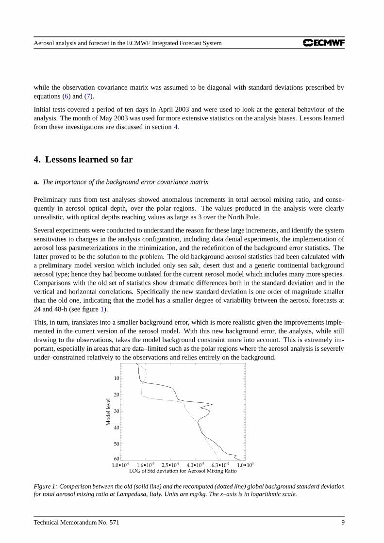
Several experiments were conducted to understand the reason for these large increments, and identify the systemsensitivities to changes in the analysis configuration, including data denial experiments, the implementation ofaerosol loss parameterizations in the minimization, and the redefinition of the background error statistics. Thelatter proved to be the solution to the problem. The old background aerosol statistics had been calculated witha preliminary model version which included only sea salt, desert dust and a generic continental backgroundaerosol type; hence they had become outdated for the current aerosol model which includes many more species.Comparisons with the old set of statistics show dramatic differences both in the standard deviation and in thevertical and horizontal correlations. Specifically the new standard deviation is one order of magnitude smallerthan the old one, indicating that the model has a smaller degree of variability between the aerosol forecasts at24 and 48-h (see figure 1).

This, in turn, translates into a smaller background error, which is more realistic given the improvements imple-mented in the current version of the aerosol model. With this new background error, the analysis, while stilldrawing to the observations, takes the model background constraint more into account. This is extremely im-portant, especially in areas that are data–limited such as the polar regions where the aerosol analysis is severelyunder–constrained relatively to the observations and relies entirely on the background.

1.0•10-6 1.6•10-5 2.5•10-4 4.0•10-3 6.3•10-2 1.0•100

LOG of Std deviation for Aerosol Mixing Ratio

60

50

40

30

20

10

Mod

el le

vel

Figure 1: Comparison between the old (solid line) and the recomputed (dotted line) global background standard deviationfor total aerosol mixing ratio at Lampedusa, Italy. Units are mg/kg. The x–axis is in logarithmic scale.



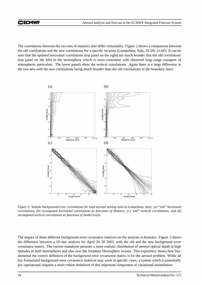
The correlations between the two sets of statistics also differ remarkably. Figure 2 shows a comparison betweenthe old correlations and the new correlations for a specific location (Lampedusa, Italy, 35.5N–12.6E). It can beseen that the updated horizontal correlations (top panel on the right) are much broader that the old correlations(top panel on the left) in the stratosphere which is more consistent with observed long–range transport ofatmospheric particulate. The lower panels show the vertical correlations. Again there is a large difference inthe two sets with the new correlations being much broader than the old correlations in the boundary layer.

0 2000 4000 6000 8000 0.100 105

distance (km)

60

50

40

30

20

10

mod

el le

vel

0.1

0.1

0.2

0.2

0.3

0.3

0.4

0.4

0.5

0.6

0.7

0.8

0.9

0 2000 4000 6000 8000 0.100 105

distance (km)

60

50

40

30

20

10

mod

el le

vel

0.1

0.1

0.1

0.1

0.2

0.2

0.2

0.3

0.4

0.5

0.6

0.7

0.8

0.9

(a) (b)

10 20 30 40 50 60

model level

60

50

40

30

20

10

mod

el le

vel

0.1

0.1 0.1

0.1

0.2

0.2

0.2

0.2

0.3

0.3

0.3

0.3

0.4

0.40.5 0.5

10 20 30 40 50 60

model level

60

50

40

30

20

10

mod

el le

vel

0.1

0.1

0.1

0.1

0.2

0.2

0.2

0.2

0.3

0.3

0.4

0.4

0.5

0.5

0.6

0.6

0.7

0.70.8

0.8

0.9

0.9

(c) (d)

Figure 2: Sample background error correlations for total aerosol mixing ratio at Lampedusa, Italy: (a) “old” horizontalcorrelations, (b) recomputed horizontal correlations as functions of distance, (c) ‘old” vertical correlations, and (d)recomputed vertical correlations as functions of model levels.

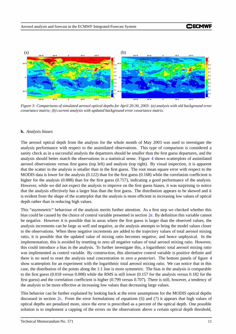
The impact of these different background error covariance matrices on the analysis is dramatic. Figure 3 showsthe difference between a 10–day analysis for April 20–30 2003, with the old and the new background errorcovariance matrix. The current reanalysis presents a more realistic distribution of aerosol optical depth at highlatitudes in both hemispheres and also over the Southern Hemisphere oceans. This experience shows how fun-damental the correct definition of the background error covariance matrix is for the aerosol problem. While adhoc formulated background error covariance matrices may work in specific cases, a system which is potentiallypre–operational requires a more robust definition of this important component of variational assimilation.



60°S60°S

0°0°

60°N60°N

120°W

120°W

60°W

60°W

0°

0°

60°E

60°E

120°E

120°E

0

0.1

0.2

0.3

0.4

0.5

0.6

0.7

0.8

0.9

1

3

60°S60°S

0°0°

60°N60°N

120°W

120°W

60°W

60°W

0°

0°

60°E

60°E

120°E

120°E

0

0.1

0.2

0.3

0.4

0.5

0.6

0.7

0.8

0.9

1

3

(a) (b)

Figure 3: Comparisons of simulated aerosol optical depths for April 20-30, 2003: (a) analysis with old background errorcovariance matrix; (b) current analysis with updated background error covariance matrix.

b. Analysis biases

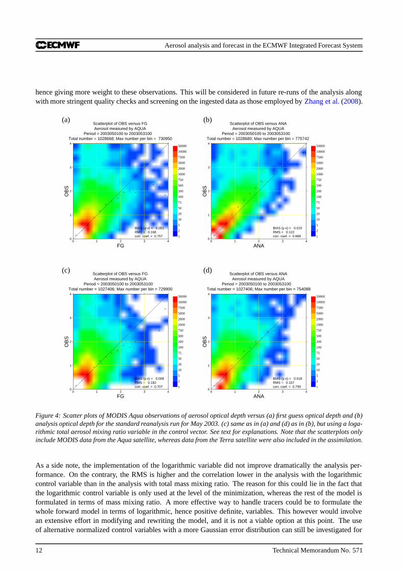
The aerosol optical depth from the analysis for the whole month of May 2003 was used to investigate theanalysis performance with respect to the assimilated observations. This type of comparison is considered asanity check as in a successful analysis the departures should be smaller than the first guess departures, and theanalysis should better match the observations in a statistical sense. Figure 4 shows scatterplots of assimilatedaerosol observations versus first guess (top left) and analysis (top right). By visual inspection, it is apparentthat the scatter in the analysis is smaller than in the first guess. The root mean square error with respect to theMODIS data is lower for the analysis (0.122) than for the first guess (0.168) while the correlation coefficient ishigher for the analysis (0.888) than for the first guess (0.757), indicating a good performance of the analysis.However, while we did not expect the analysis to improve on the first guess biases, it was surprising to noticethat the analysis effectively has a larger bias than the first guess. The distribution appears to be skewed and itis evident from the shape of the scatterplot that the analysis is more efficient in increasing low values of opticaldepth rather than in reducing high values.

This “asymmetric” behaviour of the analysis merits further attention. As a first step we checked whether thisbias could be caused by the choice of control variable presented in section 2e. By definition this variable cannotbe negative. However it is possible that in areas where the first guess is larger than the observed values, theanalysis increments can be large as well and negative, as the analysis attempts to bring the model values closerto the observations. When these negative increments are added to the trajectory values of total aerosol mixingratio, it is possible that the updated value of mixing ratio becomes negative, and hence unphysical. In theimplementation, this is avoided by resetting to zero all negative values of total aerosol mixing ratio. However,this could introduce a bias in the analysis. To further investigate this, a logarithmic total aerosol mixing ratiowas implemented as control variable. By construction, this alternative control variable is positive definite andthere is no need to reset the analysis total concentration to zero a posteriori. The bottom panels of figure 4show scatterplots for an experiment with the logarithmic total aerosol mixing ratio. We can notice that in thiscase, the distribution of the points along the 1:1 line is more symmetric. The bias in the analysis is comparableto the first guess (0.018 versus 0.008) while the RMS is still lower (0.157 for the analysis versus 0.182 for thefirst guess) and the correlation coefficient is higher (0.799 versus 0.707). There is still, however, a tendency ofthe analysis to be more effective at increasing low values than decreasing large values.

This behavior can be further explained by looking back at the error assumptions for the MODIS optical depthsdiscussed in section 2c. From the error formulations of equations (6) and (7) it appears that high values ofoptical depths are penalized more, since the error is prescribed as a percent of the optical depth. One possiblesolution is to implement a capping of the errors on the observations above a certain optical depth threshold,



hence giving more weight to these observations. This will be considered in future re-runs of the analysis alongwith more stringent quality checks and screening on the ingested data as those employed by Zhang et al. (2008).

0 1 2 3 4

FG

0

1

2

3

4

OB

S

Total number = 1028668; Max number per bin = 730950Period = 2003050100 to 2003053100

Aerosol measured by AQUAScatterplot of OBS versus FG

1

2

5

10

20

50

75

100

200

500

750

1000

2000

5000

7500

10000

50000

corr. coef. = 0.757RMS = 0.168BIAS (y-x) = 0.001

0 1 2 3 4

ANA

0

1

2

3

4

OB

S


Aerosol measured by AQUAScatterplot of OBS versus ANA

1

2

5

10

20

50

75

100

200

500

750

1000

2000

5000

7500

10000

50000


(a) (b)

0 1 2 3 4

FG

0

1

2

3

4

OB

S


Aerosol measured by AQUAScatterplot of OBS versus FG

1

2

5

10

20

50

75

100

200

500

750

1000

2000

5000

7500

10000

50000


0 1 2 3 4

ANA

0

1

2

3

4

OB

S


Aerosol measured by AQUAScatterplot of OBS versus ANA

1

2

5

10

20

50

75

100

200

500

750

1000

2000

5000

7500

10000

50000


(c) (d)

Figure 4: Scatter plots of MODIS Aqua observations of aerosol optical depth versus (a) first guess optical depth and (b)analysis optical depth for the standard reanalysis run for May 2003. (c) same as in (a) and (d) as in (b), but using a loga-rithmic total aerosol mixing ratio variable in the control vector. See text for explanations. Note that the scatterplots onlyinclude MODIS data from the Aqua satellite, whereas data from the Terra satellite were also included in the assimilation.

As a side note, the implementation of the logarithmic variable did not improve dramatically the analysis per-formance. On the contrary, the RMS is higher and the correlation lower in the analysis with the logarithmiccontrol variable than in the analysis with total mass mixing ratio. The reason for this could lie in the fact thatthe logarithmic control variable is only used at the level of the minimization, whereas the rest of the model isformulated in terms of mass mixing ratio. A more effective way to handle tracers could be to formulate thewhole forward model in terms of logarithmic, hence positive definite, variables. This however would involvean extensive effort in modifying and rewriting the model, and it is not a viable option at this point. The useof alternative normalized control variables with a more Gaussian error distribution can still be investigated for



future developments, following existing examples (Holm et al. 2002, e.g.).

5. Reanalysis results

The performance of the long reanalysis is assessed globally with comparisons with other optical depth databasesboth from space–borne sensors (i.e. the Multiangle Imaging SpectroRadiometer, MISR) and from establishedground–based sunphotometer networks (AERONET). Comparisons with MODIS data from the Aqua satelliteare also shown as reference. A more in–depth validation of the analysis which includes both optical depth andphysical property data (aerosol mass concentration) will be presented in Mangold et al. (2008).

a. Comparisons with MODIS and MISR data

The MISR instrument (Diner et al. 1998, 2005) measures 4 bands (blue, green, red and near-infrared) at differ-ent viewing angles (0., 26.1, 45.6, 60.0, and 70.5 degrees) using 9 cameras. The swath width is approximately360 km. The global coverage time is 9 days, with repeat coverage between 2 and 9 days depending on latitude.Thanks to the unique viewing geometry, MISR can measure aerosol optical depth over different reflecting sur-faces including bright surfaces as deserts. The aerosol optical depth product is quoted to have an accuracy of20% or 0.05 (whichever is larger) with greater accuracy over dark surfaces (Kahn et al. 2007). Although MISRretrievals cannot be assumed as “ground truth” as they suffer from inaccuracies related to cloud contamination,wind–speed assumptions, etc, they offer an independent platform to assess the forecast and the analysis.

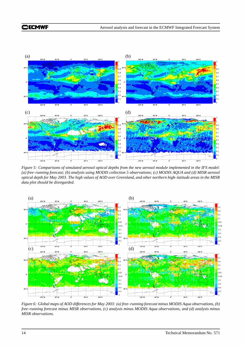
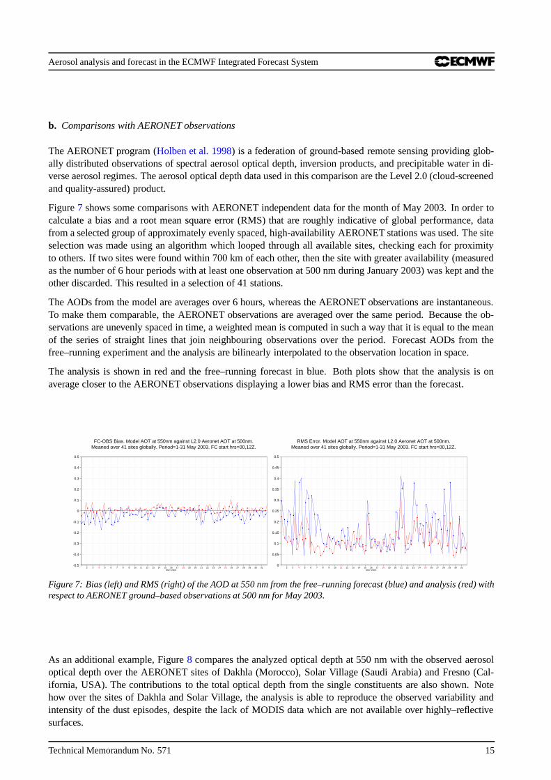
Figure 5 shows comparisons between the “free–running” forecast of aerosol optical depth without any assimila-tion, the analysis of optical depth from assimilated MODIS observations and the MISR aerosol optical depth forMay 2003. MODIS AODs are also shown as reference. Optical depth retrievals are assimilated over both landand ocean. The model aerosol optical depths are averages of three–hourly forecasts started at 00UTC from thefree–running model and from the analysis. Figure 6 shows differences between the MODIS and MISR monthlymeans with respect to the forecast and analysis optical depths. Despite some evident discrepancies, these fig-ures show that the analysis is effective in bringing the model aerosol optical depth closer to the observationsespecially in areas where the free–running forecast underestimates the AOD.

The assimilation generally improves the aerosol distribution over areas with extensive biomass burning in equa-torial West Africa. The aerosol amount in the Southern Ocean is lower in the analysis than in the free–runningforecast, also in better agreement with the observations. Other areas such as the Indian Ocean, the Indiansubcontinent and Eastern Asia dominated by anthropogenic emissions and not captured as well in the free–running simulation because of inadequate definition of the sources for these emissions, are also improved.Note, however, the overall skill of the forecast model in predicting the global distribution of the aerosol fieldsthus providing a good first–guess for the analysis. Of note is also the overall large positive bias of the analy-sis over Eurasia, and the inability of the analysis to constrain areas of large optical depths evident also in thefree-running forecast but absent in the observations (e.g. Eastern United States). The possible reasons for thisbehaviour have already been discussed in section 4b. It is, however, instructive to see the geographical distri-bution of this bias to pinpoint in which areas the analysis can be improved both through the use of observationswith better coverage and of higher quality and through refinements in the methodology.

The figures also highlight discrepancies between the two satellite products which can be as large as the largestdepartures in the free–running model and in the analysis.



60°S60°S

0°0°

60°N60°N

120°W

120°W

60°W

60°W

0°

0°

60°E

60°E

120°E

120°E

0

0.1

0.2

0.3

0.4

0.5

0.6

0.7

0.8

0.9

1

3

60°S60°S

0°0°

60°N60°N

120°W

120°W

60°W

60°W

0°

0°

60°E

60°E

120°E

120°E

0

0.1

0.2

0.3

0.4

0.5

0.6

0.7

0.8

0.9

1

3

(a) (b)

60°S60°S

0°0°

60°N60°N

120°W

120°W

60°W

60°W

0°

0°

60°E

60°E

120°E

120°E

0

0.1

0.2

0.3

0.4

0.5

0.6

0.7

0.8

0.9

1

3

60°S60°S

0°0°

60°N60°N

120°W

120°W

60°W

60°W

0°

0°

60°E

60°E

120°E

120°E

0

0.1

0.2

0.3

0.4

0.5

0.6

0.7

0.8

0.9

1

3

(c) (d)

Figure 5: Comparisons of simulated aerosol optical depths from the new aerosol module implemented in the IFS model:(a) free–running forecast; (b) analysis using MODIS collection 5 observations; (c) MODIS AQUA and (d) MISR aerosoloptical depth for May 2003. The high values of AOD over Greenland, and other northern high–latitude areas in the MISRdata plot should be disregarded.

60°S60°S

0°0°

60°N60°N

120°W

120°W

60°W

60°W

0°

0°

60°E

60°E

120°E

120°E

-1

-0.5

-0.4

-0.2

-0.1

-0.05

0.05

0.1

0.2

0.4

0.5

1

60°S60°S

0°0°

60°N60°N

120°W

120°W

60°W

60°W

0°

0°

60°E

60°E

120°E

120°E

-1

-0.5

-0.4

-0.2

-0.1

-0.05

0.05

0.1

0.2

0.4

0.5

1

(a) (b)

60°S60°S

0°0°

60°N60°N

120°W

120°W

60°W

60°W

0°

0°

60°E

60°E

120°E

120°E

-1

-0.5

-0.4

-0.2

-0.1

-0.05

0.05

0.1

0.2

0.4

0.5

1

60°S60°S

0°0°

60°N60°N

120°W

120°W

60°W

60°W

0°

0°

60°E

60°E

120°E

120°E

-1

-0.5

-0.4

-0.2

-0.1

-0.05

0.05

0.1

0.2

0.4

0.5

1

(c) (d)

Figure 6: Global maps of AOD differences for May 2003: (a) free–running forecast minus MODIS Aqua observations, (b)free–running forecast minus MISR observations, (c) analysis minus MODIS Aqua observations, and (d) analysis minusMISR observations.



b. Comparisons with AERONET observations

The AERONET program (Holben et al. 1998) is a federation of ground-based remote sensing providing glob-ally distributed observations of spectral aerosol optical depth, inversion products, and precipitable water in di-verse aerosol regimes. The aerosol optical depth data used in this comparison are the Level 2.0 (cloud-screenedand quality-assured) product.

Figure 7 shows some comparisons with AERONET independent data for the month of May 2003. In order tocalculate a bias and a root mean square error (RMS) that are roughly indicative of global performance, datafrom a selected group of approximately evenly spaced, high-availability AERONET stations was used. The siteselection was made using an algorithm which looped through all available sites, checking each for proximityto others. If two sites were found within 700 km of each other, then the site with greater availability (measuredas the number of 6 hour periods with at least one observation at 500 nm during January 2003) was kept and theother discarded. This resulted in a selection of 41 stations.

The AODs from the model are averages over 6 hours, whereas the AERONET observations are instantaneous.To make them comparable, the AERONET observations are averaged over the same period. Because the ob-servations are unevenly spaced in time, a weighted mean is computed in such a way that it is equal to the meanof the series of straight lines that join neighbouring observations over the period. Forecast AODs from thefree–running experiment and the analysis are bilinearly interpolated to the observation location in space.

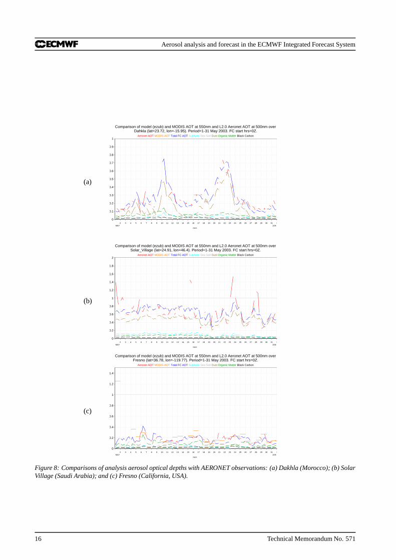
The analysis is shown in red and the free–running forecast in blue. Both plots show that the analysis is onaverage closer to the AERONET observations displaying a lower bias and RMS error than the forecast.

-0.5

-0.4

-0.3

-0.2

-0.1

0

0.1

0.2

0.3

0.4

0.5

MAY 20032 3 4 5 6 7 8 9 10 11 12 13 14 15 16 17 18 19 20 21 22 23 24 25 26 27 28 29 30 31

Meaned over 41 sites globally. Period=1-31 May 2003. FC start hrs=00,12Z.FC-OBS Bias. Model AOT at 550nm against L2.0 Aeronet AOT at 500nm.

0

0.05

0.1

0.15

0.2

0.25

0.3

0.35

0.4

0.45

0.5

MAY 20032 3 4 5 6 7 8 9 10 11 12 13 14 15 16 17 18 19 20 21 22 23 24 25 26 27 28 29 30 31

Meaned over 41 sites globally. Period=1-31 May 2003. FC start hrs=00,12Z.

RMS Error. Model AOT at 550nm against L2.0 Aeronet AOT at 500nm.

Figure 7: Bias (left) and RMS (right) of the AOD at 550 nm from the free–running forecast (blue) and analysis (red) withrespect to AERONET ground–based observations at 500 nm for May 2003.

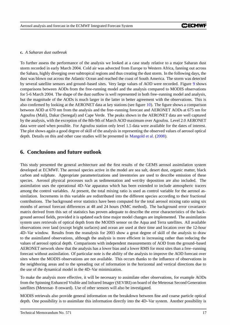
As an additional example, Figure 8 compares the analyzed optical depth at 550 nm with the observed aerosoloptical depth over the AERONET sites of Dakhla (Morocco), Solar Village (Saudi Arabia) and Fresno (Cal-ifornia, USA). The contributions to the total optical depth from the single constituents are also shown. Notehow over the sites of Dakhla and Solar Village, the analysis is able to reproduce the observed variability andintensity of the dust episodes, despite the lack of MODIS data which are not available over highly–reflectivesurfaces.



0

0.1

0.2

0.3

0.4

0.5

0.6

0.7

0.8

0.9

1

MAY2003

2 3 4 5 6 7 8 9 10 11 12 13 14 15 16 17 18 19 20 21 22 23 24 25 26 27 28 29 30 31 1JUN

Aeronet AOT MODIS AOT Total FC AOT Sulphate Sea Salt Dust Organic Matter Black Carbon

Dahkla (lat=23.72, lon=-15.95). Period=1-31 May 2003. FC start hrs=0Z.Comparison of model (ezub) and MODIS AOT at 550nm and L2.0 Aeronet AOT at 500nm over

(a)

0

0.2

0.4

0.6

0.8

1

1.2

1.4

1.6

1.8

2

MAY2003

2 3 4 5 6 7 8 9 10 11 12 13 14 15 16 17 18 19 20 21 22 23 24 25 26 27 28 29 30 31 1JUN


Solar_Village (lat=24.91, lon=46.4). Period=1-31 May 2003. FC start hrs=0Z.Comparison of model (ezub) and MODIS AOT at 550nm and L2.0 Aeronet AOT at 500nm over

(b)

0

0.2

0.4

0.6

0.8

1

1.2

1.4

MAY2003

2 3 4 5 6 7 8 9 10 11 12 13 14 15 16 17 18 19 20 21 22 23 24 25 26 27 28 29 30 31 1JUN


Fresno (lat=36.78, lon=-119.77). Period=1-31 May 2003. FC start hrs=0Z.Comparison of model (ezub) and MODIS AOT at 550nm and L2.0 Aeronet AOT at 500nm over

(c)

Figure 8: Comparisons of analysis aerosol optical depths with AERONET observations: (a) Dakhla (Morocco); (b) SolarVillage (Saudi Arabia); and (c) Fresno (California, USA).



c. A Saharan dust outbreak

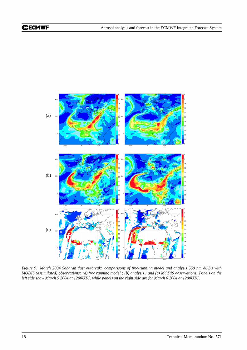
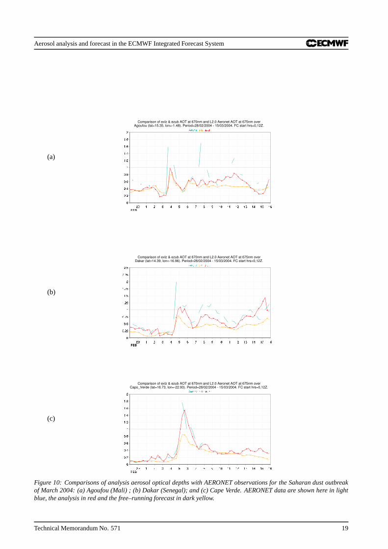
To further assess the performance of the analysis we looked at a case study relative to a major Saharan duststorm recorded in early March 2004. Cold air was advected from Europe to Western Africa, fanning out acrossthe Sahara, highly diverging over subtropical regions and thus creating the dust storm. In the following days, thedust was blown out across the Atlantic Ocean and reached the coast of South America. The storm was detectedby several satellite sensors and ground–based sites. Very large values of AOD were recorded. Figure 9 showscomparisons between AODs from the free-running model and the analysis compared to MODIS observationsfor 5-6 March 2004. The shape of the dust outflow is well represented in both free–running model and analysis,but the magnitude of the AODs is much larger in the latter in better agreement with the observations. This isalso confirmed by looking at the AERONET data at key stations (see figure 10). The figure shows a comparisonbetween AOD at 670 nm from the analysis and the free–running forecast and AERONET AODs at 675 nm forAgoufou (Mali), Dakar (Senegal) and Cape Verde. The peaks shown in the AERONET data are well capturedby the analysis, with the exception of the 8th-9th of March AOD maximum over Agoufou. Level 2.0 AERONETdata were used when possible. For Agoufou station only level 1.5 data were available for the dates of interest.The plot shows again a good degree of skill of the analysis in representing the observed values of aerosol opticaldepth. Details on this and other case studies will be presented in Mangold et al. (2008).

6. Conclusions and future outlook

This study presented the general architecture and the first results of the GEMS aerosol assimilation systemdeveloped at ECMWF. The aerosol species active in the model are sea salt, desert dust, organic matter, blackcarbon and sulphate. Appropriate parameterizations and inventories are used to describe emission of thesespecies. Aerosol physical processes such as sedimentation and wet/dry deposition are also included. Theassimilation uses the operational 4D–Var apparatus which has been extended to include atmospheric tracersamong the control variables. At present, the total mixing ratio is used as control variable for the aerosol as-similation. Increments in this variable are redistributed into the different species according to their fractionalcontributions. The background error statistics have been computed for the total aerosol mixing ratio using sixmonths of aerosol forecast differences at 48 and 24 hours (NMC method). The background error covariancematrix derived from this set of statistics has proven adequate to describe the error characteristics of the back-ground aerosol fields, provided it is updated each time major model changes are implemented. The assimilationsystem uses retrievals of optical depth from the MODIS sensor on the Aqua and Terra satellites. All availableobservations over land (except bright surfaces) and ocean are used at their time and location over the 12-hour4D–Var window. Results from the reanalysis for 2003 show a great degree of skill of the analysis to drawto the assimilated observations, although the analysis is more efficient in increasing rather than reducing thevalues of aerosol optical depth. Comparisons with independent measurements of AOD from the ground–basedAERONET network show that the analysis has a lower bias and a lower RMS for most sites than a free–runningforecast without assimilation. Of particular note is the ability of the analysis to improve the AOD forecast oversites where the MODIS observations are not available. This occurs thanks to the influence of observations inthe neighboring areas and to the spreading out of information in the horizontal and vertical directions due tothe use of the dynamical model in the 4D–Var minimization.

To make the analysis more effective, it will be necessary to assimilate other observations, for example AODsfrom the Spinning Enhanced Visible and Infrared Imager (SEVIRI) on board of the Meteosat Second Generationsatellites (Meteosat- 8 onward). Use of other sensors will also be investigated.

MODIS retrievals also provide general information on the breakdown between fine and coarse particle opticaldepth. One possibility is to assimilate this information directly into the 4D–Var system. Another possibility is



(a)

(b)

(c)

Figure 9: March 2004 Saharan dust outbreak: comparisons of free-running model and analysis 550 nm AODs withMODIS (assimilated) observations: (a) free running model ; (b) analysis ; and (c) MODIS observations. Panels on theleft side show March 5 2004 at 1200UTC, while panels on the right side are for March 6 2004 at 1200UTC.



(a)

(b)

(c)

Figure 10: Comparisons of analysis aerosol optical depths with AERONET observations for the Saharan dust outbreakof March 2004: (a) Agoufou (Mali) ; (b) Dakar (Senegal); and (c) Cape Verde. AERONET data are shown here in lightblue, the analysis in red and the free–running forecast in dark yellow.



to make use of the Angstrom parameter which also gives information on the size of the aerosol particulate fromobservations of optical depth at different wavelengths. This will require a re-thinking of the control variableand the possible introduction of more aerosol–related variables in the control vector.

A third possibility, which will be given priority, is direct assimilation of multi–wavelength reflectances. Thisdevelopment is already under way and the radiative transfer code for visible wavelengths has been alreadyprepared to be plugged into the IFS. The tangent linear and adjoint operators for the radiative transfer code (6S,Vermote et al. (1997a,b)) , necessary for the incremental variational assimilation, are under development.

The GEMS aerosol reanalysis for 2003–2004 will be completed in August 2008. An in–depth review of theresults and comparisons with yet more independent datasets is needed for a final assessment of the quality of theanalysis. This will involve several of the partners in the GEMS project. First results are however encouragingand show the capability of the analysis to draw from the observations and provide optimal initial conditionsfor improved forecasts of atmospheric aerosol fields. A follow-on project, the Monitoring Atmospheric Com-position & Climate (MACC) project, also funded by the European Commission, will explore the feasibility ofpre-operational implementation of the GEMS assimilation system for reanalysis and near real–time forecastsof aerosols. In MACC, there are also plans to make the aerosol fully interactive with the radiation scheme thusallowing us to explore fully the impact of the improved aerosol fields on the whole atmospheric system.

7. Acknowledgements

We gratefully acknowledge the developers of the GES-DISC (Goddard Earth Sciences Data and InformationServices Center) Interactive Online Visualization ANd aNalysis Infrastructure for providing an invaluable ser-vice of visualization and data processing for the MODIS and MISR data (see http://g0dup05u.ecs.nasa.gov/Giovanni/).AERONET data were obtained from the AERONET web site (http://aeronet.gsfc.nasa.gov/).

References

Bellouin, N., A. Jones, J. Haywood, and S. A. Christopher, 2008: Updated estimate of aerosol direct radiativeforcing from satellite observations and comparison against the Hadley Centre climate model, J. Geophys.Res., 113, D10205, doi:10.10292007JD009385.

Benedetti, A. and M. Fisher, 2007: Background error statistics for aerosols, Q. J. R. Meteorol. Soc., 133,391–405.

Benedetti, A. and M. Janiskova, 2008: Assimilation of MODIS cloud optical depths in the ECMWF model,Mon. Weather Rev., 136, 1727–1746.

Boucher, O., M. Pham, and C. Venkataraman, 2002: Simulation of the atmospheric sulphur cycle in the LMDGCM. Model description, model evaluation and global and European budgets, Technical Report 23, IPSL,26 pp.

Collins, W. D., P. J. Rasch, B. E. Eaton, B. V. Khattatov, and J.-F. Lamarque, 2001: Simulating aerosols usinga chemical transport model with assimilation of satellite aerosol retrievals: Methodology for INDOEX, J.Geophys. Res., 106, 7313–7336.

Courtier, P., J.-N. Thepaut, and A. Hollingsworth, 1994: A strategy for operational implementation of 4D–Var,using an incremental approach, Q. J. R. Meteor.Soc., 120, 1367–1387.



Crouzille, B., B. Gerard, J.-F. Leon, and D. Tanre, 2007: Methodology for quality assurance MODIS AerosolProducts, GEMS Technical Report, available at http://gems.ecmwf.int.

Diner, D. J., J. Beckert, T. Reilly, C. Bruegge, J. Conel, R. Kahn, J. Martonchik, T. Ackerman, R. Davies,S. Gerstl, H. Gordon, J.-P. Muller, R. Myneni, R. Sellers, B. Pinty, and M. Verstraete, 1998: Multi-angleImaging Spectroradiometer (MISR) description and experiment overview, IEEE Trans. Geosci. Rem. Sens.,36, 1072–1087.

Diner, D. J., B. H. Braswell, R. Davies, N. Gobronc, J. Hud, Y. Jine, R. A. Kahn, Y. Knyazikhin, N. Loeb, J.-P.Muller, A. W. Nolin, B. Pinty, C. B. Schaaf, G. Seizi, and J. Stroeve, 2005: The value of multiangle mea-surements for retrieving structurally and radiatively consistent properties of clouds, aerosols, and surfaces,Rem. Sens. Environ., 97, 495–518.

Errera, Q. and D. Fonteyn, 2001: Four–dimensional variational chemical assimilation of CRISTA stratosphericmeasurements, Mon. Weather Rev., 102, 12253–12265.

Fisher, M., 1998: Minimization algorithms for variational data assimilation, Seminar on Recent Developmentsin Numerical Methods for Atmospheric Modelling, 7-11 September 1998. Proceedings, ECMWF, pp. 364-385.

Fisher, M., 2003: Background error covariance modelling, Seminar on Recent developments in data assimila-tion for atmosphere and ocean, 8-12 September 2003. Proceedings, ECMWF, pp. 45-64.

Fisher, M., 2004: Generalized frames on the sphere, with application to background error covariance mod-elling, Seminar on Recent developments in numerical methods for atmospheric and ocean modelling, 6-10September 2004. Proceedings, ECMWF, pp. 87-101.

Fisher, M., 2006: “Wavelet” Jb – A new way to model the statistics of background errors, ECMWF Newsletter,106, 23–28.

Fonteyn, D., Q. Errera, M. De Maziere, G. Franssens, and D. Fussen, 2000: 4D–Var assimilation of strato-spheric aerosol satellite data, Adv. Space Res., 26, 2049–2052.

Generoso, S., F.-M. Breon, F. Chevallier, Y. Balkanski, M. Schulz, and I. Bey, 2007: Assimilation of POLDERaerosol optical thickiness into the LMDz–INCA model: Implications for the Arctic aerosol burden, J. Geo-phys. Res., 112, D02311, doi:10.1029/2005JD006954.

Holben, B. N., T. Eck, I. Slutsker, D. Tanre, J. Buis, A. Setzer, E. Vermote, J. Reagan, Y. Kaufman, T. Nakajima,F. Lavenue, I. Jankowiak, and A. Smirnov, 1998: AERONET: A federated instrument network and dataarchive for aerosol characterization, Remote Sens. Environ., 66, 1–16.

Hollingsworth, A., R. J. Engelen, C. Textor, A. Benedetti, O. Boucher, F. Chevallier, A. Dethof, H. Elbern,H. Eskes, J. Flemming, C. Granier, J. W. Kaiser, J.-J. Morcrette, P. Rayner, V.-H. Peuch, L. Rouil, M. G.Schultz, A. J. Simmons, and the GEMS consortium, 2008: The global earth–system monitoring using satel-lite and in–situ data (GEMS) project: Towards a monitoring and forecasting system for atmospheric compo-sition, Bull. Amer. Meteor. Soc., To appear.

Holm, E., E. Andersson, A. Beljaars, P. Lopez, J.-F. Mahfouf, A. J. Simmons, and J.-N. Thepaut, 2002: Assim-ilation and Modelling of the Hydrological Cycle: ECMWF’s Status and Plans, Technical Memorandum 383,ECMWF, 55 pp.



Kahn, R. A., M. J. Garay, D. L. Nelson, K. K. Yau, M. A. Bull, B. J. Gaitley, J. V. Martonchik, andR. C. Levy, 2007: Satellite-derived aerosol optical depth over dark water from MISR and MODIS:Comparisons with AERONET and implications for climatological studies, J. Geophys. Res., 112,D18205,doi:10.1029/2006JD008175.

Kahnert, M., 2008: Variational data analysis of aerosol species in a regional CTM: Background error covarianceconstraint and aerosol optical observation operators, Tellus B.

Lewtas, J., 2007: Air pollution combustion emissions: Characterization of causative agents and mechanismsassociated with cancer, reproductive, and cardiovascular effects, Mutat. Res. - Rev. Mut. Res., 636, 95–133.

Lopez, P. and E. Moreau, 2005: A convection scheme for data assimilation: Description and initial tests, Q. J.R. Meteorol. Soc., 131, 409–436.

Mangold, A., H. De Backer, B. De Paepe, S. Dewitte, M. Schulz, Y. Balkanski, N. Huneeus, I. Chiapello,D. Ceburnis, C. O’Dowd, H. Flentje, S. Kinne, O. Boucher, J.-J. Morcrette, A. Benedetti, J. W. Kaiser,L. Jones, and the GEMS–AER team, 2008: Aerosol analysis and forecast in the ECMWF Integrated ForecastSystem. Part III: Evaluation, In preparation.

Morcrette, J.-J., A. Benedetti, O. Boucher, P. Bechtold, A. Beljaars, M. Rodwell, S. Serrar, M. Suttie, A. Tomp-kins, and A. Untch, 2006: GEMS–Aerosols at ECMWF, Seminar on Global Monitoring of the Earth-System,5-9 September 2005. Proceedings, ECMWF, pp. 255-270.

Morcrette, J.-J., O. Boucher, D. Salmond, L. Jones, P. Bechtold, A. Beljaars, A. Benedetti, A. Bonet,A. Hollingsworth, J. W. Kaiser, M. Razinger, S. Serrar, A. J. Simmons, M. Suttie, A. Tompkins, A. Untch,and the GEMS–AER team, 2008: Aerosol analysis and forecast in the ECMWF Integrated Forecast System:Forward modelling, Technical report, ECMWF Technical Memorandum No. XXX, in preparation.

Niu, T., S. L. Gong, G. F. Zhu, H. L. Liu, X. Q. Hu, C. H. Zhou, and Y. Q. Wang, 2008: Data assimilation ofdust aerosol observations for the CUACE/dust forecasting system, Atmos. Chem. Phys., 8, 3473–3482.

Parrish, D. F. and J. C. Derber, 1992: The National Meteorological Center’s spectral statistical–interpolationanalysis system, Mon. Weather Rev., 120, 1747–1763.

Rasch, P. J., W. D. Collins, and B. E. Eaton, 2001: Understanding the Indian Ocean Experiment (INDOEX)aerosol distributions with an aerosol assimilation, J. Geophys. Res., 106, 7337–7355.

Reddy, M. S., O. Boucher, N. Bellouin, M. Schulz, Y. Balkanski, J.-L. Dufresne, and M. Pham, 2005:Estimates of global multicomponent aerosol optical depth and direct radiative perturbation in the Lab-oratoire de Meteorologie Dynamique General Circulation Model, J. Geophys. Res., 110, D10S16,doi:10.1029/2004JD004757.

Remer, L. A., Y. J. Kaufman, D. Tanre, S. Mattoo, D. A. Chu, J. V. Martins, R.-R. Li, C. Ichoku, R. C. Levy,R. G. Kleidman, T. F. Eck, E. Vermote, and B. N. Holben, 2005: The MODIS aerosol algorithm, productsand validation, J. Atmos. Sci., 62, 947–973.

Thompson, M. C., A. M. Molesworth, M. H. Djingarey, K. R. Yameogo, F. Belanger, and L. E. Cuevas, 2006:Potential of environmental models to predict meningitis epidemics in africa, Trop. Med. Int. Health, 11,781–788.

Tompkins, A. M., 2005: A revised cloud scheme to reduce the sensitivity to vertical resolution, Technicalmemorandum, ECMWF.



Tompkins, A. M. and M. Janiskova, 2004: A cloud scheme for data assimilation: Description and initial tests,Q. J. R. Meteorol. Soc., 130, 2495–2517.

Tremolet, Y., 2005: Incremental 4D–Var convergence study, Technical Memorandum 469, ECMWF, 34 pp.

Tsigaridis, K., Y. Balkanski, M. Schulz, and A. Benedetti, 2008: Global error maps of aerosol optical properties:an error propagation analysis, Atmos. Chem. Phys., Submitted.

Vermote, E. D., D. Tanre, J. L. Deuze, M. Herman, and J.-J. Morcrette, 1997a: Second Simulation of theSatellite Signal in the Solar Spectrum: an overview, IEEE Trans. Geosci. Remote Sens., 35, 675–686.

Vermote, E. D., D. Tanre, J. L. Deuze, M. Herman, and J.-J. Morcrette, 1997b: Second Simulation of theSatellite Signal in the Solar Spectrum: an overview, 6S, User guide version 2, 53 pp.

Weaver, C., A. da Silva, M. Chin, P. Ginoux, O. Dubovik, D. Flittner, A. Zia, L. Remer, B. Holben, andW. Gregg, 2007: Direct insertion of MODIS radiances in a global aerosol transport model, J. Atmos. Sci., 64,808–826.

Zhang, J. and J. S. Reid, 2006: MODIS aerosol product analysis for data assimilation: Assess-ment of over–ocean level 2 aerosol optical thickness retrievals, J. Geophys. Res., 111, D22207,doi:10.1029/2005JD006898.

Zhang, J., J. S. Reid, D. L. Westphal, N. L. Baker, and E. J. Hyer, 2008: A system for operational aerosoloptical depth assimilation over global oceans, J. Geophys. Res., 113, D10208, doi:10.1029/2007JD009065.


aerosol analysis and forecast ecmwf integrated forecast

Documents