aeroelastic stability of a 3dof system based on quasi
TRANSCRIPT

University of Birmingham
Aeroelastic stability of a 3DOF system based onquasi-steady theory with reference to inertialcouplingHe, Mingzhe; macdonal, john
DOI:10.1016/j.jweia.2017.10.013
License:Creative Commons: Attribution-NonCommercial-NoDerivs (CC BY-NC-ND)
Document VersionPublisher's PDF, also known as Version of record
Citation for published version (Harvard):He, M & macdonal, J 2017, 'Aeroelastic stability of a 3DOF system based on quasi-steady theory with referenceto inertial coupling', Journal of Wind Engineering and Industrial Aerodynamics, vol. 171.https://doi.org/10.1016/j.jweia.2017.10.013
Link to publication on Research at Birmingham portal
Publisher Rights Statement:https://doi.org/10.1016/j.jweia.2017.10.013
General rightsUnless a licence is specified above, all rights (including copyright and moral rights) in this document are retained by the authors and/or thecopyright holders. The express permission of the copyright holder must be obtained for any use of this material other than for purposespermitted by law.
•Users may freely distribute the URL that is used to identify this publication.•Users may download and/or print one copy of the publication from the University of Birmingham research portal for the purpose of privatestudy or non-commercial research.•User may use extracts from the document in line with the concept of ‘fair dealing’ under the Copyright, Designs and Patents Act 1988 (?)•Users may not further distribute the material nor use it for the purposes of commercial gain.
Where a licence is displayed above, please note the terms and conditions of the licence govern your use of this document.
When citing, please reference the published version.
Take down policyWhile the University of Birmingham exercises care and attention in making items available there are rare occasions when an item has beenuploaded in error or has been deemed to be commercially or otherwise sensitive.
If you believe that this is the case for this document, please contact [email protected] providing details and we will remove access tothe work immediately and investigate.
Download date: 28. Nov. 2021

Journal of Wind Engineering & Industrial Aerodynamics 171 (2017) 319–329
Contents lists available at ScienceDirect
Journal of Wind Engineering & Industrial Aerodynamics
journal homepage: www.elsevier .com/locate/ jweia
Aeroelastic stability of a 3DOF system based on quasi-steady theory withreference to inertial coupling
Mingzhe He *,1, John Macdonald
Department of Civil Engineering, University of Bristol, BS8 1TR, UK
A R T I C L E I N F O
Keywords:3DOF gallopingQuasi-steady theoryInertial couplingEigenvalue problem
* Corresponding author.E-mail addresses: [email protected] (M. He), john.ma
1 Now at the University of Birmingham. Address: Univ
https://doi.org/10.1016/j.jweia.2017.10.013Received 27 April 2017; Received in revised form 10 Oct
0167-6105/© 2017 Elsevier Ltd. All rights reserved.
A B S T R A C T
This paper investigates the galloping stability of a two-dimensional three-degree-of-freedom (3DOF) system withan eccentric shape, such as an iced cable or power transmission line, incorporating inertial coupling along withthe aerodynamic damping. The inertial coupling is a result of the offset of the centre of mass with respect to theelastic centre. A theoretical model is firstly constructed for the derivation of the aerodynamic damping matrix,based on quasi-steady theory, as well as the inertial coupling components in the mass matrix. The model is thenemployed to investigate the effects on the aeroelastic stability of the system of incorporating the inertial couplingand the results are compared with both dynamic test results and predictions from previous models. The com-parisons indicate that even small eccentricity can lead to significant change of the stability of the system, for bothdetuned and perfectly tuned natural frequencies of the different degrees of freedom. For a system with perfectlytuned natural frequencies, and neglecting structural damping, analytical solutions of the eigenfrequencies andeigenvectors allowing for the inertial coupling, are derived for the case of no wind. Subsequently, an approximatesolution is found for the prediction of the galloping stability of a system coupled by the aerodynamic damping aswell as the inertial coupling. Finally, the approximate solution is verified against numerical results using exampleswith two cross-section shapes, showing excellent agreement.
1. Introduction
Galloping has been a major problem for decades for slender struc-tures, especially transmission lines and bridge cables. One of the mostcommon methods of predicting galloping is to use theoretical models,based on quasi-steady theory, which only requires static aerodynamiccoefficients measured in wind tunnel tests. Den Hartog (1932) proposed asimple expression to forecast across-wind galloping of transmission lineswith ice accretion, which is still widely used today. However, it is onlyvalid for wind normal to the body and only considers thesingle-degree-of-freedom (1DOF) case.
It is common to consider aerodynamic couplings between the verticaland torsional motion of a section in flutter analysis. Flutter instability is awell-known phenomenon which could cause structural failure of aircraftwings, long-span bridges, etc. The stability is normally assessed by anumerical approach based on flutter derivatives which, similar to theaerodynamic coefficients, can also be measured in wind tunnel tests, butmore dynamic tests must be involved. Chen and Kareem (2006) suc-cessfully derived a closed-form solution of coupled flutter instability of
[email protected] (J. Macdonaldersity of Birmingham, Civil Engineeri
ober 2017; Accepted 11 October 201
long-span bridges, which showed good agreement with test results. Itshould be noted that flutter derivatives are functions of reduced velocity,which is rather low for large bodies such as bridge decks, leading to a lowaccuracy of quasi-steady theory. However, if cross-sections with muchsmaller diameters are considered, such as cables and power lines,quasi-steady theory, as well as the term “galloping”, is more applicable.Also, the static aerodynamic coefficients are much easier to measure incomparison with flutter derivatives.
For iced transmission line conductors, Den Hartog proved that the iceaccretion plays a significant role in modifying the aerodynamics,potentially leading to aerodynamic instability in the pure across-winddirection. However, if the torsional motion is also considered, the ef-fects of inertial coupling due to the eccentric mass of the ice coating couldbe equally important. There has been extensive literature on two-degree-of-freedom (2DOF) galloping (coupled plunge and torsion), based onquasi-steady theory (Slater, 1969; Blevins and Iwan, 1974; Modi andSlater, 1983; Yu et al., 1995a, 1995b), as reviewed by Blevins (1994) andPaïdoussis et al. (2010). Slater (1969) was the first to investigate thisproblem using a right angle section, with both aerodynamic and inertial
).ng Building; Engineering South Campus, Edgbaston, Birmingham, B15 2TT, UK.
7

Fig. 1. The 2 dimensional model of the 3DOF system.
M. He, J. Macdonald Journal of Wind Engineering & Industrial Aerodynamics 171 (2017) 319–329
coupling. Interaction between torsion and plunge was expected, due tothe misalignment of the mass centre and shear centre. However, onlydistinct vertical or torsional motion was identified in the dynamic ex-periments, which was believed to be because the inertial coupling wasweak. A similar cross-section was also studied by Blevins and Iwan(1974), who neglected inertial coupling from the outset and focused oninternally resonant and non-resonant cases. Yu et al. (1995a) used a2DOF model representing a single conductor with ice coating to not onlyidentify the onset of the coupled transverse-torsion galloping but also toinvestigate the significance of the eccentricity. In their companion work(Yu et al., 1995b), the methodology was applied to periodic motions.Although it is generally not possible to derive simple analytical solutionsfor such complicated problem, they managed to show the trends of thegalloping onset threshold due to the eccentricity in a tabular manner forpractical purposes.
Jones (1992) was the first to investigate the 2DOF translationalgalloping problem (along- and across-wind) experimentally and analyt-ically for a perfectly tuned system and found that aerodynamic couplingbetween the two degrees of freedom was important. Macdonald andLarose (2006) generalised the Den Hartog criterion by allowing forReynolds number effects and three-dimensional geometry of the inclinedcable in a skew wind. They then extended it to apply to 2DOF trans-lational galloping (Macdonald and Larose, 2008a,b). They provided aclosed-form solution for the minimum structural damping required toprevent galloping of a system with the same natural frequencies in thetwo planes. The companion paper looked at some detuning cases basedon numerical solutions. Meanwhile, Carassale et al. (2005) derivedequivalent expressions of the aerodynamic damping matrix, butexcluding and questioning the relevance of Reynolds number effects.Furthermore, Luongo and Piccardo (2005) proposed an analyticalapproximation for the onset of galloping of a 2DOF translational systemwith arbitrary natural frequencies, employing a perturbation approach.The above analyses were reviewed by Nikitas and Macdonald (2014).However, inertial coupling was not considered in any of them.
The afore-mentioned research implies that there could be interactionsbetween heave, sway and torsion simultaneously, which poses the ne-cessity of studying coupled 3DOF galloping. Yu et al. (1993a,b) devel-oped the work by Jones (1992) and established a galloping threshold,based on the Routh-Hurwitz criterion, for a 3DOF system with mass
320
eccentricity. Wang and Lilien (1998) studied single and bundled trans-mission lines covered by ice coating and similarly proposed a modeltaking all three degrees of freedom into account. However, both thesestudies concentrated on multi-span effects rather than a simple criterionfor the onset of galloping. The Routh-Hurwitz criterion utilised by Yuet al. (1993a,b) is rather inefficient for determining how stable or un-stable the system is. In the latter study, the galloping stability was eval-uated by numerical time history analysis.
Very few dynamic wind tunnel tests on 2 or 3DOF galloping havebeen reported in the literature. Chabart and Lilien (1998) carried outboth static and dynamic wind tunnel tests on a heavily iced cable whichshed some light on the galloping mechanism of a 3DOF cable with largeeccentricity. Gjelstrup and Georgakis (2011) extended the model byMacdonald and Larose (2008a, b) to include the torsional degree offreedom and also the case where the mass centre and elastic centre do notcoincide. The theoretical galloping threshold was determined using theRouth-Hurwitz criterion and reasonable comparisons were found withthe observations from the experiments by Chabart and Lilien (1998).Gjelstrup et al. (2012) further carried out some experiments to examinethe galloping stability of bridge cables and hangers with various iceshapes. The test results were also comparedwith the theoretical model byGjelstrup and Georgakis (2011). However, the experiments only allowedfor vertical and torsional motions andmass eccentricity was not explicitlyconsidered. More recent contributions on 3DOF galloping include workby Piccardo et al. (2014) who presented the full aerodynamic dampingmatrix in a more general form, while Demartino and Ricciardelli (2015)compared various existing quasi-steady models for galloping, using windtunnel measurements for bridge cables and hangers with ice accretion,shedding some light on the application of each model. He andMacdonald(2016) extended the work by Nikitas and Macdonald (2014) and rigor-ously studied 3DOF galloping of a system coupled only by aerodynamicdamping and proposed a simple closed-form solution for galloping of aperfectly tuned 3DOF system. They also numerically investigated theeffects of the tuning of the structural natural frequencies (He and Mac-donald, 2015).
The aim of this paper is to extend the previous 3DOF analytical modelby He and Macdonald (2016) to include inertial coupling. Firstly, theinertial coupling terms in the mass matrix are derived in the same way asin Gjelstrup and Georgakis (2011). Then, the significance of the inertialcoupling for the galloping behaviour is investigated. Subsequently,having found analytical solutions to the eigenvalue problem for aneccentric 3DOF system, without wind or structural damping, approxi-mate analytical solutions are found for the galloping stability of thesystem in the presence of wind. Finally, the approximate analytical so-lutions are validated against conventional numerical solutions for thesame system.
2. 3DOF model and equations of motion
Recently, He and Macdonald (2016) presented a 2-dimensional 3DOFmodel and derived the aerodynamic damping matrix in a simple form,including all three degrees of freedom, based on quasi-steady theory.Inertial coupling was excluded, implying coincidence of the elastic centre(O) and mass centre (G), which is applicable for sections with symmet-rical geometry and lightly iced sections with a negligible offset of thecentre of mass. A modified model is presented herein to include theinertia effects, as illustrated in Fig. 1, where G is offset from O. Theincorporation of all three degrees of freedom results in a difficulty ofquasi-steady theory, namely suitable treatment of the rotational velocity.The approach employed follows the common approach in the literature(Slater, 1969; Blevins and Iwan, 1974; Nakamura and Mizota, 1975;Blevins, 1994; Gjelstrup and Georgakis, 2011; He and Macdonald, 2016),where an aerodynamic centre is defined to emulate the effect of therotational velocity on the aerodynamic forces using the wind velocityrelative to that point.
Fig. 1 shows the definitions of all the geometric parameters. x and y

M. He, J. Macdonald Journal of Wind Engineering & Industrial Aerodynamics 171 (2017) 319–329
indicate the directions of the principal structural axes of the system and θis the rotation of the cross-section, measured between the x axis and areference line on the body (the dashed line in Fig. 1, fixed to the cross-sectional shape). θ consists of two parts, namely the static rotation ofthe shape, θ0 (e.g. due to the mean wind load or the weight of accretedice), and the dynamic component, θd. The structural stiffness of eachdegree of freedom is denoted kx, ky and kθ, which can also be expressed asmω2
x , mω2y and Jθω2
θ , respectively. m is the mass per unit length of thestructure and Jθ is the polar mass moment of inertia per unit length aboutpoint O. ωx; ωy and ωθ are the angular natural frequencies of theuncoupled structural system in each degree of freedom. α0 is the anglebetween the wind direction and the x axis while α represents the anglebetween the wind direction and the body reference line (α ¼ α0þθ). Themass centre (G) differs from the elastic centre (O), for example, due to theice accretion, and is positioned at a radius Lg at an angle αg from the bodyreference line. Similarly, the offset distance and angle of the aerodynamiccentre (A) from the elastic centre are respectively defined by La and γrfrom the reference line. It should be noted that the aerodynamic centre(A) in Fig. 1 is shown in an arbitrary position for illustration of thegeneral case. The specific point used for the numerical examples later inthe current paper is defined in Section 3.1.
The position of any point on the shape can be defined in the absolutecoordinate system, indicated by X and Y axes in Fig. 1. The absolutecoordinates of the centre of mass are:
X ¼ x� Lgcos�αg þ θ
�; Y ¼ yþ Lgsin
�αg þ θ
�(1)
Hence,
_X ¼ _xþ Lg_θ sin
�αg þ θ
�; _Y ¼ _yþ Lg
_θ cos�αg þ θ
�(2)
The equations of motion can then be obtained by applying the Euler-Lagrange equation, which involves the kinetic (T) and potential (V) en-ergy, expressed as:
T ¼ 12m�_X2 þ _Y
2�þ 12JG _θ
2(3)
V ¼ 12kxx2 þ 1
2kyy2 þ 1
2kθθ2 (4)
With the Lagrangian defined as L¼ T-V, the force on the body in the xdirection, excluding the damping component, satisfies:
Fx ¼ ∂∂t
�∂L∂ _x
�� ∂L
∂x(5)
The force in the y direction, Fy , and themoment on the body Fθ, can beexpressed similarly. Hence, the full equations of motion, with dampingforces included, are:
Fx ¼ m€xþ 2mωxζx _xþ kxxþ mLg
�€θ sin
�αg þ θ
�þ _θ2cos
�αg þ θ
� �(6)
Fy ¼ m€yþ 2mωyζy _yþ kyyþ mLg
�€θ cos
�αg þ θ
�� _θ2sin
�αg þ θ
� �(7)
Fθ ¼ Jθ €θ þ 2mωθζθ _θ þ kθθ þ mLg€xsin�αg þ θ
�þ mLg€ycos�αg þ θ
�(8)
where ζx, ζy and ζθ are the structural damping ratios for each degree offreedom and Jθ ¼ JG þmL2g ¼ mr2 is the polar mass moment of inertiaper unit length about point O, as mentioned earlier and r is the radius ofgyration about O. JG is the polar mass moment of inertia per unit length
about point G. It should be noted that the terms associated with _θ2can be
neglected when linearising the force at the initial steady state condition.The equations of motion can be written in matrix form as:
321
M€x þ Cs €x þ Kx ¼ F (9)
where
M ¼ m
24 1 0 Lg sin
�αg þ θ
�0 1 Lg cos
�αg þ θ
�Lg sin
�αg þ θ
�Lg cos
�αg þ θ
�r2
35,
Cs ¼242mωxζx 0 0
0 2mωyζy 00 0 2Jθωθζθ
35, K ¼
24mω2
x 0 00 mω2
y 00 0 Jθω2
θ
35,
x ¼8<:
xyθd
9=;, F ¼
8<:
FxFyFθ
9=;.
Neglecting any applied forces other than the aerodynamic forces dueto the motion of the body in the wind, and linearising the force vectorwith respect to the velocity vector, about the static equilibrium config-uration (in where x ¼ 0), the force vector can be expressed as
F ¼ �Cax (10)
Ca is the aerodynamic damping matrix, given by:
Ca ¼24 cxxa cxya cxθacyxa cyya cyθacθxa cθya cθθa
35 ¼
266666664
�∂Fx
∂ _x�∂Fx
∂ _y�∂Fx
∂ _θ
�∂Fy
∂ _x�∂Fy
∂ _y�∂Fy
∂ _θ
�∂Fθ
∂ _x�∂Fθ
∂ _y�∂Fθ
∂ _θ
377777775
_x¼ _y¼ _θ¼θd¼0
(11)
which, based on quasi-steady theory and for any wind direction andorientation of the body, has been shown to be (He andMacdonald, 2016):
Ca ¼ ρDU2
242CD 2CL
�C0
L þ CD
� �CL �C0
D
�0 0
2CL �2CD
�CL � C'
D
� ��C'
L þ CD
�0 0
0 0 0 0 2DCM DC0M
35
�
26666664
c2 cs Lasαθγ c�cs �s2 �Lasαθγ ss2 �cs �Lacαθγ scs �c2 �Lacαθγ cc s Lasαθγ�s c Lacαθγ
37777775
(12)
where ρ is the density of air, D is a reference dimension of the body andCD, CLand CM are, respectively, the static drag, lift and moment co-efficients of the cross-section, which are taken to be only functions of theangle of attack, α. The primes indicate derivatives with respect to theangle of attack. In addition, c ¼ cos α0; s ¼ sin α0; cαθγ ¼cos ðα0 þθ0 þ γrÞ and sαθγ ¼ sin ðα0 þ θ0 þ γrÞ.
The equations of motion and the asymmetric mass matrix due to ec-centricity are equivalent to those derived by Gjelstrup and Georga-kis (2011).
It should be emphasised that the force coefficients and their de-rivatives should be evaluated at the angle between the wind and theshape in the static equilibrium configuration about which the dynamicstability is considered, i.e. at α0 þ θ0 (¼ α for θd ¼ 0). To address thestability, i.e. the conditions for the onset of galloping, it is sufficient touse the linearised representation of the aerodynamic forces above.
He and Macdonald (2016) found that the determinant of the 3DOFquasi-steady aerodynamic damping matrix Ca is always zero, which is notgenerally true for any pair of two DOFs. The reason is that the motion ofthe aerodynamic centre due to the rotational velocity can be decomposedinto components in the x and y directions, leading to the third column ofthe 3� 3 aerodynamic damping matrix being a linear combination of the

Fig. 2. Static force coefficients for a cable with heavy ice (Chabart and Lilien, 1998).
Fig. 3. Stability predicted by the present model and Gjelstrup model, and as observed inthe dynamic tests. U ¼ 9 m/s; fx ¼ 0.960 Hz, fy ¼ 0.845 Hz; fθ ¼ 0.865 Hz; ζx ¼ ζy ¼ 0.8%;ζθ ¼ 3.0%.
M. He, J. Macdonald Journal of Wind Engineering & Industrial Aerodynamics 171 (2017) 319–329
first and second columns.In addition, there are aerodynamic stiffness terms, namely �∂F
∂θ
����θd¼0
,
which could have an effect, especially for cross-sections with large sideratios or width to depth ratios. However, for the present work, the cross-sections investigated are normally referred to as compact cross-sections,i.e., the side ratios are normally less than 2, for which the effects ofaerodynamic stiffness are usually assumed to be negligible compared tothe structural stiffness (Gjelstrup and Georgakis, 2011). Therefore, theaerodynamic stiffness is excluded in the present analysis.
3. The effects of inertial coupling
In this section, the 3DOF model is first examined for its applicabilityin comparison with wind tunnel tests results (Chabart and Lilien, 1998)and a similar 3DOF model by Gjelstrup and Georgakis (2011), referred toas the Gjelstrup model hereinafter. Afterwards, the effects of the inertialcoupling are investigated using the proposed 3DOF model.
322
3.1. Application of the proposed model
Due to a lack of experimental data of 3DOF dynamic tests of compactsections, the present analysis is largely based on data and results from thewind tunnel tests conducted by Chabart and Lilien (1998). The test sec-tion was an aluminium alloy conductor covered by thick silicone ice,giving large eccentricity. The force coefficients and the ice shape with theaerodynamic force sign conventions are depicted in Fig. 2:
Apart from the inertial coupling and aerodynamic damping, the 3DOFmodel developed by Gjelstrup and Georgakis (2011) also took into ac-count both wind skew angle and Reynolds number effects. The stability isdetermined by the Routh-Hurwitz criterion, which, as discussed earlier,is convenient in finding out whether the system is stable or not but rathercumbersome for quantifying how unstable the system is. In addition, thismodel only succeeded in predicting part of the unstable region observedin the tests, i.e. from 25� to 45�, 70�–135� and 170�–180�, whilegalloping was found to occur from 20� to 180� in the dynamicexperiments.
Through eigenvalue analysis, the stability of the proposed model,described by Eqs. (9), (10) and (12), is identified. Fig. 3 shows thegalloping stability of the system, over the full range of angles of attacktested in the wind tunnel, as predicted by the present model and theGjelstrup model. The observed unstable region in the experiments is alsoindicated. The stability is assessed in terms of the non-dimensionalaerodynamic damping coefficient, S3D, which is also employed in thegalloping analyses by Nikitas and Macdonald (2014) and He and Mac-donald (2016). It is defined as
S3D ¼ 4mωnζaρDU
(13)
where ζa indicates the effective aerodynamic damping ratio, which iscomparable to the structural damping ratios (ζx, ζy and ζθ). A negativesign of S3D or ζa means galloping would occur if insufficient structuraldamping is provided. It should be noted the curves in Fig. 3 represent themost critical solution of the eigenvalue results, i.e. the minimum S3D of allthree modes.
From Fig. 3, it is manifest that the proposed model predicts the wholeunstable region observed in the experiments, which was reported byChabart and Lilien (1998). It should be noted that all the parameters inthe present analysis are consistent with those in (Gjelstrup and

Fig. 4. Comparison of the galloping stability of the aeroelastically coupled cross-sectionwith and without inertial coupling. Well-detuned system. fx ¼ 0.96 Hz, fy ¼ 0.85 Hz;fθ ¼ 1.54 Hz; ζx ¼ ζy ¼ 0.8%; ζθ ¼ 3.0%; U ¼ 9 m/s.
Fig. 5. Comparison of the galloping stability of the aeroelastically coupled cross-sectionwith and without inertial coupling. Vertical and torsional frequencies closely tuned.fx ¼ 0.995 Hz, fy ¼ 0.845 Hz; fθ ¼ 0.865 Hz; ζx ¼ ζy ¼ 0.8%; ζθ ¼ 3.0%; U ¼ 9 m/s.
Fig. 6. Comparison of the galloping stability of the aeroelastically coupled cross-sectionwith and without inertial coupling. All three frequencies perfectly tunedfx ¼ fy ¼ fθ ¼ 0.845 Hz; ζx ¼ ζy ¼ 0.8%; ζθ ¼ 3.0%; U ¼ 9 m/s.
M. He, J. Macdonald Journal of Wind Engineering & Industrial Aerodynamics 171 (2017) 319–329
Georgakis, 2011) to be more comparable, except the definition of theaerodynamic centre. Moreover, their definitions of some of their anglesare unclear, hence the reproduction of their results has to be undercertain assumptions. Nevertheless, it seems that the main reason for thedifferent predictions by the two similar models is the definition of theaerodynamic centre. Gjelstrup and Georgakis (2011) used the leading
323
edge of the shape as the aerodynamic centre. However, after comparingseveral ways of defining the aerodynamic centre according to previousliterature, it is found in the present analysis that the aerodynamic centreis chosen to be a fixed point on the principal axis in the x direction with Laequal to the largest offset of the perimeter of the section from the elasticcentre (i.e. the sum of the radius of the cable and the greatest ice thick-ness). Hence, the aerodynamic centre is basically the leading edge of theshape at 0� angle of attack and remains unchanged throughout theanalysis. It is clear that with this assumption the results are greatlyimproved. In light of the fact that there is no theoretical position wherethe aerodynamic centre should be, it is suggested that for this particularcross-section, the chosen point appears to be the best choice.
3.2. Galloping stability of systems with and without inertial coupling
In order to further explore the significance of the inertial coupling, aseries of numerical analyses are carried out, which can be divided intotwo approaches. The first approach is to compare two systems: (i) onlyaeroelastically coupled by the aerodynamic damping and (ii) coupledstructurally by the inertial coupling as well as aeroelastically by theaerodynamic damping. The second approach, covered in the next sectioninvolves varying the offset of the centre of mass. The same cross-sectiontested by Chabart and Lilien (1998) is employed as an example. In theirtests, two different plunge-to-torsion frequency ratios (fy/fθ) were ach-ieved through changing the position of the vertical springs.
Fig. 4 shows the numerical results of the setup with fy/fθ ¼ 0.55, interms of the minimum non-dimensional aerodynamic damping coeffi-cient, with and without the inclusion of inertial coupling.
The case illustrated in Fig. 4 represents a well-detuned system. Thefirst impression is that the incorporation of the inertial coupling has onlylimited influence on the stability of the system. The two curves followsimilar trends and the magnitudes are also close.
Fig. 5 shows the results for the same cross-section but with the ver-tical and torsional frequencies very close to each other (fy/fθ ¼ 0.98). Ascan be seen, the stability curves of the two systems also follow a similartrend with varying angles of attack. However, the difference in magni-tude is often quite large in this case, especially around the most criticalangles of attack, 35�. Including the mass eccentricity can lead to thestability curve shifting towards the stable or unstable side, depending onthe position of the mass centre. For this particular shape, it implies thesystem would be more stable when the ice is at the upstream side. Butwhen the ice accretion is on the leeward side, the inertial coupling seemsto destabilise the system.
For the case with all the structural natural frequencies of the systemperfectly tuned, with all the other parameters identical, the stability isshown in Fig. 6. Again, the stability curves, representing the two systems,show large discrepancies caused by the inertial coupling. For example, atthe most unstable angle (around 35�), the system coupled by both inertialcoupling and aerodynamic damping becomes much less unstable. Inaddition, from 90� to 160�, if the inertial coupling is not included, thesystem should be stable. However, once inertial coupling is incorporated,the system is only stable in the range of ~125�–135�. It is also clear thatthere are similarities between Figs. 5 and 6, especially for α < 90�. Theclosely tuned and perfectly tuned cases are of particular interest forbundled conductors since they often have very close natural frequenciesto each other.
In summary, the inertial coupling clearly has a great effect on thegalloping stability, especially when the natural frequencies of the systemare close.
3.3. The effects of varying inertial coupling
In this section, the effects of inertial coupling are investigated byvarying the mass ratio between the ice and the cable, leading to a varyingoffset distance of the total mass centre from the elastic centre. Thefundamental idea is to keep the shape, as well as the total mass of the

Fig. 7. Effects of varying the position of the centre of mass based on the cross-section from (Chabart and Lilien, 1998) at different angles of attack: (a, b). α ¼ 10�; (c, d). α ¼ 30�; (e, f).α ¼ 160�. U ¼ 9 m/s; fx ¼ 0.995 Hz, fy ¼ 0.845 Hz; fθ ¼ 0.865 Hz ζx ¼ ζy ¼ ζθ ¼ 0.
M. He, J. Macdonald Journal of Wind Engineering & Industrial Aerodynamics 171 (2017) 319–329
cross-section unchanged, by only artificially changing the mass ratio ofthe ice to the whole cross-section to vary the location of the centre ofmass (G) of the overall body. As has been defined earlier, the distancebetween the centre of mass the whole body (G) and the shear centre (O),which is also the centre of mass of the circular cylinder, is Lg. Herein, thedistance between the centre of mass of the ice and that of the cable (O) isdenoted herein by LT. Hence, the mass ratio between the ice and thewhole cross-section can be represented by Lg/LT.
Fig. 7 illustrates the effects of increasing the inertial coupling at threedifferent angles of attack. The figures on the left side show the effect onthe stability of the each mode of the system, in terms of the non-dimensional aerodynamic damping coefficient, against the shift of the
324
mass centre. The plots on the right side indicate the changes of the cor-responding modal frequencies.
In general, Fig. 7 implies that the inertia effects due to the varyingoffset distance of the overall centre of mass can be linked to the effects offrequency tuning. For example, in Fig. 7(a), the stability curves, repre-senting modes 1 and 2 accordingly, are far apart when the mass centre isnot offset but quickly start to come together as Lg/LT increases until about0.1. This indicates a detuning effect which can be verified by the corre-sponding modal frequency plot of Fig. 7(b). It is clear that the modalfrequencies of modes 1 and 2 are initially very close to each other.Including the inertial coupling causes the modal frequencies of the modes1 and 2 to diverge, while the stability of the modes rapidly converges.

Fig. 8. Aerodynamic coefficients for Lightly iced cable with small eccentricity (Gjelstrup et al., 2012) (ice shape figure reproduced with kind permission of Techno-Press).
M. He, J. Macdonald Journal of Wind Engineering & Industrial Aerodynamics 171 (2017) 319–329
This is consistent with the classic pattern of tuning a 2DOF system, as hasbeen shown by Nikitas and Macdonald (2014), i.e., at the perfect tuningpoint the stability curves of the two modes will be in either an attractingor repelling pattern and any detuning leads to the solutions changingasymptotically to the single-degree-of-freedom (SDOF) solutions. As theoffset distance continues to increase, the frequency of mode 2 ceasesgrowing around Lg/LT � 0.15 and begins to approach 1 Hz asymptoti-cally, while the frequency of mode 3, close to 1 Hz from Lg/LT ¼ 0, startsto increase. It seems that these two curves exhibit a typical “frequencyveering” phenomenon. He andMacdonald (2015) investigated the effectsof frequency tuning of the 3DOF system, coupled by aerodynamicdamping, and suggested that frequency veering occurs whenever theso-called “complex motion” occurs. The term “complex motion” has beenused by many researchers (Jones, 1992; Carassale et al., 2005; Mac-donald and Larose, 2008a; Nikitas and Macdonald, 2014; He and Mac-donald, 2016) to signify a special solution of a coupled system withresonant structural natural frequencies, where two modes with differentmodal frequencies have identical stability. Using a perturbationapproach, Luongo and Piccardo (2005) identified the similarity betweenthis so-called “complex response” and double Hopf bifurcation. As can beseen from the stability curves (Fig. 7(a)), the stability curves corre-sponding to the two veering modes, indeed intersect at the frequencyveering point. It is noted that modes 2 and 3 cross at Lg/LT � 0.05 butwithout veering, which is believed to be due to the frequencies of modes1 and 2 are almost identical while the modal frequency of mode 3 can beregarded as detuned. Hence, the interaction between modes 1 and 2 ismore essential.
Similar features of both stability and frequency curves can also befound in Fig. 7(c) and (d). Fig. 7(c) indicates modes 1 and 2 have a similartuning pattern to those in Fig. 7(a), i.e. a repelling pattern when thesystem is perfectly tuned. Once the eccentricity is introduced, the modalfrequencies of these two modes are detuned, causing the stability curvesto move quickly towards each other. As the mass centre continues to shiftaway, frequency veering occurs between modes 2 and 3 leading to thecrossing of the corresponding stability curves. It is very interesting tonotice the rapid changes of the stability of certain modes even when theeccentricity introduced is very small. For instance, mode 2, which is nearthe stability boundary but stable, quickly becomes very unstable whenthe eccentricity is only about 5%.
Fig. 7(e) and (f) again illustrate both the tuning effects and the fre-quency veering phenomenon, as explained above. This time, the close
325
tuning of modes 1 and 2 leads to an attracting pattern of the stabilitycurves. When the inertial coupling is increased, modal frequencies ofmodes 1 and 2 are detuned, leading to the divergence of the corre-sponding stability curves. As a result, the stability curve of mode 2 goesdown to lower values away from the stability boundary as the eccen-tricity increases. When the inertial coupling is strong enough, frequencyveering occurs, resulting in the stability curves of mode 2 reversing backtowards the stability boundary. It intersects with the curve representingthe stability of mode 3, which is also an expected feature for fre-quency veering.
Another important feature of all of the stability curves is that evenvery small eccentricity can cause a significant change of the system sta-bility. In all of the plots, the stability of at least one of the modes changesrapidly as the position of the centre of mass starts to move away from theshear centre. It is important to note that the stability of the system canexperience considerable changes due to the inertial coupling only, for nochange in the aerodynamics, even for a small offset of the centre of mass.For instance, if a small protuberance is attached to a circular cylinder, it iswell known that the modification of the aerodynamics could lead toinstability. However, the associated small offset of the centre of masscould also be important in changing the stability. This possibility is nowexplored further with a lightly iced cable, the centre of mass of which ismanually offset by a very small distance.
Gjelstrup et al. (2012) conducted a series of wind tunnel tests oncircular cylinders covered by four different ice coatings. The test setupallowed for plunge and torsion but the horizontal motion was fullyrestrained. The test results were used to compare with their analyticalmodel (Gjelstrup and Georgakis, 2011), using the Routh-Hurwitz crite-rion. The lightly iced cable employed in the present analysis is the shapeII, plotted in Fig. 8, which has a mean ice thickness of only 1.4% of thediameter of the cable. Consequently, the effects of mass eccentricity wereconsidered to be negligible in their numerical examinations reported inGjelstrup et al. (2012). The aerodynamic coefficients are also providedin Fig. 8.
Firstly, an eigenvalue analysis is conducted using the proposed modelbut only including the across-wind (y) and torsional (θ) degrees offreedom, based on this shape with all the parameters consistent with theanalysis by Gjelstrup et al. (2012). Then, the same analysis is repeatedbut a small offset of the centre of mass will be numerically created tointroduce inertial coupling. The offset distance is 5% of the cable diam-eter from the elastic centre (shear centre). As a result, the mass matrix

Fig. 9. Comparison of galloping stability of a lightly iced cable with and without masseccentricity. U ¼ 41 m/s; fy ¼ 1.63 Hz; fθ ¼ 4.99 Hz; ζy ¼ 0.8%; ζθ ¼ 4.3%.
Fig. 10. Comparison of galloping stability of a lightly iced cable with and without masseccentricity: (a) the stability expressed in terms of the non-dimensional aerodynamicdamping; (b) modal frequencies. U ¼ 41 m/s; fy ¼ fθ ¼ 1.63 Hz; ζy ¼ 0.8%; ζθ ¼ 4.3%.
M. He, J. Macdonald Journal of Wind Engineering & Industrial Aerodynamics 171 (2017) 319–329
becomes non-diagonal. Also, the mass polar moment of inertia is slightlydifferent. The results of both cases are compared and illustrated in Fig. 9.It should be mentioned that S2D, equivalent to S3D in the preceding sec-tion, is used herein since the model is a 2DOF one.
326
As can be seen from Fig. 9 for a system with well separated naturalfrequencies, the incorporation of such small eccentricity seems to havenegligible influence on the across-wind dominated mode while there is asignificant effect on the torsion dominated mode. Despite the differencefor the torsion dominated mode, it remains stable for all angles of attack,while in any case, the across-wind dominated mode is unstable forcertain angles of attack. Considering the modal frequencies, the changeswere minor. There was a negligible shift in the frequency of the across-wind dominated mode and the frequency of the torsion dominatedmode changed only up to 1.05% due to the inertial coupling.
Following the preceding analysis, another case is also investigatedwhere the same system has resonant structural natural frequencies,illustrated in Fig. 10. The figure shows that for the perfectly tuned sys-tem, the stability curves of both modes show a noticeable differencebetween the two cases, i.e., with and without small eccentricity. Withregard to the overall stability of the system, the behaviour at the mostunstable angles of attack, namely about ±35�, is almost the same for bothcases. However, including eccentricity may lead to different unstableregions when the system is not far from the stability boundary, i.e., whenS2D is close to 0. For example, when only aerodynamic damping isincluded, the system is slightly unstable at about 65�. After introducingsmall eccentricity, at 65�, the system is just on the stability boundary,which means it should be neutrally stable. On the other hand, atapproximately �65�, the aerodynamically coupled case indicates thesystem is clearly stable but once the mass offset is introduced, the systembecomes unstable at that angle in the torsion dominated mode.
In summary, the inertial coupling can exert significant influence onthe stability of a system for both perfectly tuned and detuned cases. Evenif the offset of the centre of mass is small, the effects on the stability canstill be substantial.
4. Analytical investigation of a perfectly tuned system withinertial coupling
The preceding sections have demonstrated the importance of the in-ertial coupling for both detuned and perfectly tuned systems based onnumerical eigenvalue analysis. It could be more useful for practicalpurposes and more insightful to have analytical solutions. However, dueto the complex nature of the problem, it is difficult to obtain simpleanalytical solutions for a system with arbitrary tuning. In the first part ofthis section, analytical expressions of the eigenfrequencies along with theassociated eigenvectors are derived for a perfectly tuned 3DOF systemstructurally coupled by mass inertia without the presence of wind. Asmentioned earlier, the perfectly tuned case is of use for bundled con-ductors which have very close natural frequencies for all 3 degrees offreedom. Thenceforth, an approximate solution is proposed in the secondpart for the onset of galloping for a perfectly tuned 3DOF system coupledby aerodynamic damping and inertial coupling. The structural dampingratio in the whole section is neglected for simplicity since the structuraldamping only makes the system more stable.
4.1. Without the presence of wind
With the structural matrices defined as for Eq. (9), the eigenvalues ofa system with only inertial coupling, with no wind or structural dampingcan be obtained by��� ω2Mþ K
�� ¼ 0 (14)
where ω is the eigenfrequency of the inertially coupled system. It shouldbe noted the structural natural frequencies without coupling, namelyωx; ωy and ωθ, are all set to be ωn for a perfectly tuned system. Hence,Eq. (14) can be expanded into:
�ω2 � ω2
n
���Lg � r
�ω2 þ rω2
n
���Lg þ r
�ω2 � rω2
n
� ¼ 0 (15)

Fig. 11. The effects of the inertial coupling on the system eigenfrequencies of a perfectlytuned 3DOF system with no wind.
M. He, J. Macdonald Journal of Wind Engineering & Industrial Aerodynamics 171 (2017) 319–329
The three solutions for the eigenvalues (ω), ω1; ω2, ω3 along withtheir associated eigenvectors, ϕ1, ϕ2, ϕ3, are:
ω21 ¼ r
r�Lgω2n , ϕ1 ¼
8<:
�rsin�αg þ θ0
��rcos
�αg þ θ0
�1
9=;;
Fig. 12. Trajectories of motion in the 3 modes: (a) Mode 1; (b) Mode 2; (c) Mode 3. The ‘rotavibration cycle.
327
ω22 ¼ ω2
n , ϕ2 ¼8<:
�cot�αg þ θ0
�10
9=;;
ω23 ¼ r
rþLgω2n , ϕ3 ¼
8<:
rsin�αg þ θ0
�rcos
�αg þ θ0
�1
9=;.
An illustration of the normalised eigenfrequencies with varying Lg/ris shown in Fig. 11, which demonstrates the significance of the iner-tial coupling.
As can be seen, ω3 decreases as the inertial coupling increases whileω1 has an opposite trend. Based on the eigenvectors, the trajectories ofthe motion in each mode are plotted in Fig. 12, for an offset angle of thecentre of mass of 30� as an example. Mode 1 (Fig. 12(a)) represents arotation about a point that is between the centre of mass (G) and theelastic centre (O), which moves closer to G with increasing mass offset.Therefore, polar moment of inertia about the point decreases, so themodal frequency should increase with increasing offset. On the otherhand, the eigenvector of Mode 3 (Fig. 12(c)) indicates motion about apoint the same distance from O but in the opposite direction. Hence, thepolar moment of inertia about the point increases and the natural fre-quency decreases as the inertial coupling increases. Mode 2 (Fig. 12(b))involves purely translational motion along the line (OG) connecting thetwo centres, which is not affected by the inertial coupling, giving a modalfrequency equal to the uncoupled natural frequencies of the system. It isalso evident that the amplitude ratio of the translational motions ofModes 1 and 3 always follow the same relation, i.e. the horizontalamplitude over the vertical one always equals tanðαg þ θ0Þ.
tion’ lines show snapshots of the orientation of the body at equal time intervals over the

Fig. 13. Comparison between the proposed closed-form solutions and the numerical re-sults for a heavily iced cable (Chabart and Lilien, 1998). fx ¼ fy ¼ fθ ¼ fn ¼ 1 Hz,ζx ¼ ζy ¼ ζθ ¼ 0, U ¼ 9 m/s. Offset distance of the centre of mass is 7.7% of the cablediameter.
M. He, J. Macdonald Journal of Wind Engineering & Industrial Aerodynamics 171 (2017) 319–329
4.2. Approximate solutions for galloping of a 3DOF body coupled by bothinertial coupling and aerodynamic damping
With the above insights of the effects of inertial coupling with nowind, the more general case, incorporating both inertial coupling andaerodynamic damping, is examined. Using the same 3DOFmodel, as wellas the mass and stiffness matrices, the space state matrix A, after addingthe aerodynamic damping matrix, is:
A ¼
0 I�M�1⋅K �M�1⋅Ca
(16)
The structural damping is neglected in the present analysis to makethe problem tractable, noting that the structural damping is normallysmall in practice (Chen and Kareem, 2006) and that adding structuraldamping will always increase the stability.
Following He and Macdonald (2016), the aerodynamic dampingmatrix can be expressed as:
Ca ¼ ρDU2
24 1 0 00 1 00 0 r
35Sa
24 1 0 00 1 00 0 r
35 (17)
where Sa is a non-dimensional matrix, given by (He and Macdon-ald, 2016):
Sa ¼24 Sxx Sxy SxθSyx Syy SyθSθx Sθy Sθθ
35
¼24 2CD 2CL
�C0
L þ CD
� �CL � C0
D
�0 0
2CL �2CD
�CL � C0
D
� ��C0
L þ CD
�0 0
0 0 0 0 2κCM κC0M
35
�
26666664
c2 cs εsαθγ c�cs �s2 �εsαθγ ss2 �cs �εcαθγ scs �c2 �εcαθγ cc s εsαθγ�s c εcαθγ
37777775
(18)
where κ ¼ D=r and ε ¼ La=r.The characteristic polynomial of the system is given by:
jA� λIj ¼ 0 (19)
where λ are the complex eigenvalues of the problem.
328
Eq. (19) is a lengthy 6th order equation, which theoretically could bedecomposed into the form of the product of three quadratic equations,each representing one of the three modes with complex conjugate roots.Therefore, an approximate equation in such a form is proposed:
�λ2 þ b1⋅λþ r
r � Lgω2
n
��λ2 þ b2⋅λþ ω2
n
��λ2 þ b3⋅λþ r
r þ Lgω2
n
�� 0
(20)
The eigenfrequencies, i.e. the third term in each pair of brackets in Eq.(20), assuming low damping, are estimated to be equal to those for the nowind condition, calculated from Eq. (15). This assumption is in agree-ment with Chen and Kareem (2006). They found that for low levels ofdamping, which is generally the case in flutter or galloping analysis, theaerodynamically uncoupled natural frequencies can be used to estimatethe coupled modal frequencies in presence of wind.
After expanding Eq. (20), the coefficients of each order of λ are rep-resented by mathematical combinations of three unknowns, b1, b2 and b3.By comparing these coefficients with those in the characteristic poly-nomial derived from Eq. (19), a set of equations can be established tosolve for those unknowns. From observation of the expanded Eq. (20),the coefficients of λ5 and λ are linear relations of the three unknowns.Furthermore, the coefficient of λ3 also contains linear relations of thethree unknowns, with only one higher order term, i.e. b1b2b3. This term isequivalent to the product of the real part of all the eigenvalues. Since thereal part of the eigenvalues gives the overall damping of each degree offreedom of the system, which is generally fairly small, the product ofthem is hence quite close to zero. The corresponding coefficient in Eq.(19) contains an equivalent “higher order” term, namely the determinantof the damping matrix (jCaj) which is always 0. Thus, b1b2b3 and jCaj canbe cancelled out from both sides of the equation. Consequently, a thirdlinear relation between the three unknowns can be obtained. By solvingthe three linear equations in b1, b2 and b3, the real part of the eigenvalues(λR) of each mode can be derived, since only the instability threshold is ofinterest, as
λR1 ¼ �b12� ρDU
8mr�
r � Lg
� ðd1 þ d2Þ (21)
λR2 ¼ �b22� �ρDU
4m
�Sxx þ Syy þ Sθθ þ d1
�(22)
λR3 ¼ �b32� ρDU
8mr�
r þ Lg
� ðd1 � d2Þ (23)
where
d1 ¼ ��Sxxsin2
�αg þ θ
�þ Syycos2�αg þ θ
�þ �Sxy þ Syx
�sin
�αg þ θ
�cos
�αg þ θ
�þ Sθθ�
d2 ¼ �Sθy þ Syθ
�cos
�αg þ θ
�þ ðSxθ þ SθxÞsin�αg þ θ
�
For stability, a positive real part indicates an unstable mode while anegative value means the mode is stable. Hence, the galloping stabilitycan be assessed using the maximum of the three simple expressions (Eqs.(21)–(23)), or the minimum one, if the equivalent non-dimensionalaerodynamic damping coefficients are used (S3D ¼ �4mλR=ρDU).
4.3. Validation and application of the proposed analytical solutions
In this section, the proposed approximate solution is validated againstthe exact numerical results. The two examples, employed in the previoussections, namely the iced cables tested by Chabart and Lilien (1998) andGjelstrup et al. (2012), are investigated.
Firstly, the cable with large ice coating examined by Chabart andLilien (1998) is utilised. Since the proposed approximate solutions onlyapply for perfectly tuned structural natural frequencies (before the in-ertial coupling is introduced), they are all set to be fn ¼ 1 Hz. This is quite
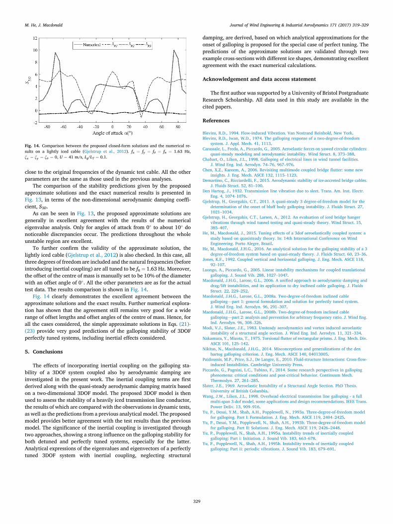
Fig. 14. Comparison between the proposed closed-form solutions and the numerical re-sults on a lightly iced cable (Gjelstrup et al., 2012). fx ¼ fy ¼ fθ ¼ fn ¼ 1.63 Hz,ζx ¼ ζy ¼ ζθ ¼ 0, U ¼ 41 m/s, Lg/LT ¼ 0.1.
M. He, J. Macdonald Journal of Wind Engineering & Industrial Aerodynamics 171 (2017) 319–329
close to the original frequencies of the dynamic test cable. All the otherparameters are the same as those used in the previous analyses.
The comparison of the stability predictions given by the proposedapproximate solutions and the exact numerical results is presented inFig. 13, in terms of the non-dimensional aerodynamic damping coeffi-cient, S3D.
As can be seen in Fig. 13, the proposed approximate solutions aregenerally in excellent agreement with the results of the numericaleigenvalue analysis. Only for angles of attack from 0� to about 10� donoticeable discrepancies occur. The predictions throughout the wholeunstable region are excellent.
To further confirm the validity of the approximate solution, thelightly iced cable (Gjelstrup et al., 2012) is also checked. In this case, allthree degrees of freedom are included and the natural frequencies (beforeintroducing inertial coupling) are all tuned to be fn ¼ 1.63 Hz. Moreover,the offset of the centre of mass is manually set to be 10% of the diameterwith an offset angle of 0�. All the other parameters are as for the actualtest data. The results comparison is shown in Fig. 14.
Fig. 14 clearly demonstrates the excellent agreement between theapproximate solutions and the exact results. Further numerical explora-tion has shown that the agreement still remains very good for a widerange of offset lengths and offset angles of the centre of mass. Hence, forall the cases considered, the simple approximate solutions in Eqs. (21)-(23) provide very good predictions of the galloping stability of 3DOFperfectly tuned systems, including inertial effects considered.
5. Conclusions
The effects of incorporating inertial coupling on the galloping sta-bility of a 3DOF system coupled also by aerodynamic damping areinvestigated in the present work. The inertial coupling terms are firstderived along with the quasi-steady aerodynamic damping matrix basedon a two-dimensional 3DOF model. The proposed 3DOF model is thenused to assess the stability of a heavily iced transmission line conductor,the results of which are compared with the observations in dynamic tests,as well as the predictions from a previous analytical model. The proposedmodel provides better agreement with the test results than the previousmodel. The significance of the inertial coupling is investigated throughtwo approaches, showing a strong influence on the galloping stability forboth detuned and perfectly tuned systems, especially for the latter.Analytical expressions of the eigenvalues and eigenvectors of a perfectlytuned 3DOF system with inertial coupling, neglecting structural
329
damping, are derived, based on which analytical approximations for theonset of galloping is proposed for the special case of perfect tuning. Thepredictions of the approximate solutions are validated through twoexample cross-sections with different ice shapes, demonstrating excellentagreement with the exact numerical calculations.
Acknowledgement and data access statement
The first author was supported by a University of Bristol PostgraduateResearch Scholarship. All data used in this study are available in thecited papers.
References
Blevins, R.D., 1994. Flow-induced Vibration. Van Nostrand Reinhold, New York.Blevins, R.D., Iwan, W.D., 1974. The galloping response of a two-degree-of-freedom
system. J. Appl. Mech. 41, 1113.Carassale, L., Freda, A., Piccardo, G., 2005. Aeroelastic forces on yawed circular cylinders:
quasi-steady modeling and aerodynamic instability. Wind Struct. 8, 373–388.Chabart, O., Lilien, J.L., 1998. Galloping of electrical lines in wind tunnel facilities.
J. Wind Eng. Ind. Aerodyn. 74–76, 967–976.Chen, X.Z., Kareem, A., 2006. Revisiting multimode coupled bridge flutter: some new
insights. J. Eng. Mech. ASCE 132, 1115–1123.Demartino, C., Ricciardelli, F., 2015. Aerodynamic stability of ice-accreted bridge cables.
J. Fluids Struct. 52, 81–100.Den Hartog, J., 1932. Transmission line vibration due to sleet. Trans. Am. Inst. Electr.
Eng. 4, 1074–1076.Gjelstrup, H., Georgakis, C.T., 2011. A quasi-steady 3 degree-of-freedom model for the
determination of the onset of bluff body galloping instability. J. Fluids Struct. 27,1021–1034.
Gjelstrup, H., Georgakis, C.T., Larsen, A., 2012. An evaluation of iced bridge hangervibrations through wind tunnel testing and quasi-steady theory. Wind Struct. 15,385–407.
He, M., Macdonald, J., 2015. Tuning effects of a 3dof aeroelastically coupled system: astudy based on quasisteady theory. In: 14th International Conference on WindEngineering. Porto Alegre, Brazil.
He, M., Macdonald, J.H.G., 2016. An analytical solution for the galloping stability of a 3degree-of-freedom system based on quasi-steady theory. J. Fluids Struct. 60, 23–36.
Jones, K.F., 1992. Coupled vertical and horizontal galloping. J. Eng. Mech. ASCE 118,92–107.
Luongo, A., Piccardo, G., 2005. Linear instability mechanisms for coupled translationalgalloping. J. Sound Vib. 288, 1027–1047.
Macdonald, J.H.G., Larose, G.L., 2006. A unified approach to aerodynamic damping anddrag/lift instabilities, and its application to dry inclined cable galloping. J. FluidsStruct. 22, 229–252.
Macdonald, J.H.G., Larose, G.L., 2008a. Two-degree-of-freedom inclined cablegalloping—part 1: general formulation and solution for perfectly tuned system.J. Wind Eng. Ind. Aerodyn. 96, 291–307.
Macdonald, J.H.G., Larose, G.L., 2008b. Two-degree-of-freedom inclined cablegalloping—part 2: analysis and prevention for arbitrary frequency ratio. J. Wind Eng.Ind. Aerodyn. 96, 308–326.
Modi, V.J., Slater, J.E., 1983. Unsteady aerodynamics and vortex induced aeroelasticinstability of a structural angle section. J. Wind Eng. Ind. Aerodyn. 11, 321–334.
Nakamura, Y., Mizota, T., 1975. Torsional flutter of rectangular prisms. J. Eng. Mech. Div.ASCE 101, 125–142.
Nikitas, N., Macdonald, J.H.G., 2014. Misconceptions and generalizations of the denhartog galloping criterion. J. Eng. Mech. ASCE 140, 04013005.
Païdoussis, M.P., Price, S.J., De Langre, E., 2010. Fluid-structure Interactions: Cross-flow-induced Instabilities. Cambridge University Press.
Piccardo, G., Pagnini, L.C., Tubino, F., 2014. Some research perspectives in gallopingphenomena: critical conditions and post-critical behavior. Continuum Mech.Thermodyn. 27, 261–285.
Slater, J.E., 1969. Aeroelastic Instability of a Structural Angle Section. PhD Thesis.University of British Columbia.
Wang, J.W., Lilien, J.L., 1998. Overhead electrical transmission line galloping - a fullmulti-span 3-dof model, some applications and design recommendations. IEEE Trans.Power Deliv. 13, 909–916.
Yu, P., Desai, Y.M., Shah, A.H., Popplewell, N., 1993a. Three-degree-of-freedom modelfor galloping. Part I: Formulation. J. Eng. Mech. ASCE 119, 2404–2425.
Yu, P., Desai, Y.M., Popplewell, N., Shah, A.H., 1993b. Three-degree-of-freedom modelfor galloping. Part II: Solutions. J. Eng. Mech. ASCE 119, 2426–2448.
Yu, P., Popplewell, N., Shah, A.H., 1995a. Instability trends of inertially coupledgalloping: Part i: Initiation. J. Sound Vib. 183, 663–678.
Yu, P., Popplewell, N., Shah, A.H., 1995b. Instability trends of inertially coupledgalloping: Part ii: periodic vibrations. J. Sound Vib. 183, 679–691.