aerodynamicanalysisofthenrel5-mwwind turbine using vortex...
TRANSCRIPT
−2
−1
0
1
2
310
2030
4050
6070
0
500
1000
1500
2000
2500
3000
3500
4000
4500
radius [m]chord [m]
Pre
ssure
[N
/m2]
500
1000
1500
2000
2500
3000
3500
4000
Aerodynamic Analysis of the NREL 5-MWWind
Turbine using Vortex Panel MethodMaster’s thesis in Fluid Mechanics
KATHARINA MAIREAD SCHWEIGLER
Department of Applied Mechanics
Division of Fluid Dynamics
CHALMERS UNIVERSITY OF TECHNOLOGY
Gothenburg, Sweden 2012
Master’s thesis 2012:17


MASTER’S THESIS IN FLUID MECHANICS
Aerodynamic Analysis of the NREL 5-MW Wind Turbine
using Vortex Panel Method
KATHARINA MAIREAD SCHWEIGLER
Department of Applied Mechanics
Division of Fluid Dynamics
CHALMERS UNIVERSITY OF TECHNOLOGY
Gothenburg, Sweden 2012

Aerodynamic Analysis of the NREL 5-MW Wind Turbine using Vortex Panel
Method
KATHARINA MAIREAD SCHWEIGLER
c© KATHARINA MAIREAD SCHWEIGLER, 2012
Master’s thesis 2012:17
ISSN 1652-8557
Department of Applied Mechanics
Division of Fluid Dynamics
Chalmers University of Technology
SE-412 96 Gothenburg
Sweden
Telephone: +46 (0)31-772 1000
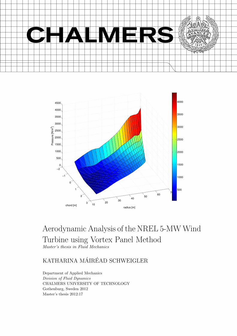
Cover:
Pressure distribution of a turbine blade of the NREL 5-MW wind turbine
Chalmers Reproservice
Gothenburg, Sweden 2012

Aerodynamic Analysis of the NREL 5-MW Wind Turbine using Vortex Panel
Method
Master’s thesis in Fluid Mechanics
KATHARINA MAIREAD SCHWEIGLER
Department of Applied Mechanics
Division of Fluid Dynamics
Chalmers University of Technology
Abstract
The purpose of this study was to investigate if panel methods can be used to
examine aerodynamic loads on wind turbine blades. Another aim was to find out
the differences between the Lifting Surface Method, the Vortex Panel Method (a
number of panels along the chord) and the Reduced Vortex Panel Method (one
panel along the chord) when applied to horizontal axis wind turbines.
Panel methods use vortex filaments or rings to model the surface of a solid
body and the wake behind the wind turbine. Therefore, a grid was laid on
the blades and the wake. That way for every blade the influence of all wakes
and blades was taken into account. In this thesis the wind profile was uniform.
Furthermore, incompressible, frictionless flow was assumed.
The results for the NREL 5-MW wind turbine revealed that the Lifting Surface
Method and the Reduced Vortex Panel Method produce similar force distributions
along the blade (from root to tip). The forces obtained with the Vortex Panel
Method are not only higher but also more accurate compared to Computational
Fluid Dynamics, Blade Element Momentum and General Unsteady Vortex Particle
data for the same blade.
The principal conclusion was, the Vortex Panel Method is a suitable tool to
investigate the aerodynamic loads on horizontal axis wind turbines with three
blades.
Keywords: Vortex Panel Method, Wind turbine, Aerodynamics, Thin Airfoil
Theory, Lifting Surface Method, Induced velocity, NREL 5-MW
i
Zusammenfassung
Der Zweck dieser Arbeit war es, zu untersuchen, ob Panel Methoden zur Be-
stimmung der aerodynamischen Lasten auf Rotorblatter von Windenergieanlagen
genutzt werden konnen. Ein weiteres Ziel dieser Arbeit war es, die Unterschiede
zwischen der Lifting Surface Methode, der Vortex Panel Methode (einige Panele
entlang der Sehne) und der Reduzierten Vortex Panel Methode (ein Panel ent-
lang der Sehne), auf Windenergieanlagen mit horizontaler Achse angewandt, zu
untersuchen.
Panel Methoden verwenden Vortexlinien oder -ringe, um die Oberflache eines
festen Korpers und die Wirbelschleppe hinter dem Windrad zu modellieren.
Daher wurde ein Gitter auf den Rotorblattern und der Schleppe erstellt. Damit
konnte der Einfluss von allen Wirbelschleppen und Blattern fur jedes Blatt
berucksichtigt werden. In dieser Arbeit war das Windprofil homogen. Desweiteren
wurde inkompressible, reibungsfreie Stromung angenommen.
Die Ergebnisse fur die NREL 5-MW Windturbine haben gezeigt, dass die
Lifting Surface Methode und die Reduzierte Vortex Panel Methode ahnliche
Kraftverteilungen entlang der Rotorblatter (von der Nabe bis zur Spitze) erge-
ben. Die Krafte, die die Vortex Panel Methode lieferte, waren nicht nur hoher,
sondern auch genauer, verglichen mit Computational Fluid Dynamics, Blade
Element Momentum und General Unsteady Vortex Particle Daten fur das gleiche
Rotorblatt.
Die wichtigste Schlussfolgerung war, dass die Vortex Panel Methode ein gu-
tes Werkzeug ist, um die aerodynamischen Lasten auf Windenergieanlagen mit
horizontaler Achse und drei Rotorblattern zu untersuchen.
ii

Acknowledgements
First of all I would like to thank Professor Lars Davidson for kindly accepting me
as a master’s thesis student at the Division of Fluid Mechanics and for letting me
feel welcome the whole time together with the Staff of the Division.
I would also like to thank Professor Martin Gabi for giving me the chance to work
on this topic.
Very special thanks go to my supervisor Hamidreza Abedi for his support and
guidance throughout this thesis. He has always given optimistic comments and
constructive advice. Thanks to Christoffer Jarpner and Ayyoob Zarmehri for
their helpful ideas and the supply with CFD data.
Thanks to Pablo Mosquera Michaelsen for supporting me during the last weeks
of my thesis in Germany. Mrs. Kolmel, thanks for always being so friendly and
helpful with all formalities.
For financial support, I thank the Friedrich-Ebert-Stiftung, without whose help
all of this would not have been possible.
My final words go to my family and friends. Without their support from Germany
and during their stay in Sweden it would have been very hard to write this thesis
abroad.
iii

Nomenclature
Roman letters
ai influence coefficient
b span length
c chord length
cL lift coefficient
i grid node counter along chord
j grid node counter along span
k grid node counter along wake
l variable along a vortex filament
n normal
q velocity
r radius / distance from control point to one end of a vortex filament
u velocity component in x-direction
v velocity component in y-direction
w velocity component in z-direction
Ai influence coefficients matrix
AR aspect ratio
F force
L lift
L′ lift per unit span
R maximal radius
Greek letters
α angle of attack
β angle between two wake consecutive grid nodes in the wake
γ vorticity, vortex strength or circulation of a single vortex element
ρ density of air
φ velocity potential
ω rotation of a fluid
Γ vortex strength distribution
iv

Subscripts
b body
eff effective
i induced
m number of vortex rings
n number of control points
nor normal to rotor plane
rot rotational
tang tangential to rotor plane
T.E. trailing edge
θ tangential to vortex filament
∞ free stream
Abbreviations
BEM Blade Element Momentum
CFD Computational Fluid Dynamics
GENUVP GENeral Unsteady Vortex Particle
NREL National Renewable Energy Laboratory
RVPM Reduced Vortex Panel Method
VPM Vortex Panel Method
v
Contents
Abstract i
Zusammenfassung ii
Acknowledgements iii
Nomenclature iv
Contents vi
1 Introduction 1
1.1 Motivation . . . . . . . . . . . . . . . . . . . . . . . . . . . . . . . . . 1
1.2 Objective . . . . . . . . . . . . . . . . . . . . . . . . . . . . . . . . . . 1
1.3 Outline of the thesis . . . . . . . . . . . . . . . . . . . . . . . . . . . . 1
2 Fundamentals 3
2.1 Terminology . . . . . . . . . . . . . . . . . . . . . . . . . . . . . . . . 3
2.2 Lift . . . . . . . . . . . . . . . . . . . . . . . . . . . . . . . . . . . . 5
2.3 Governing equations . . . . . . . . . . . . . . . . . . . . . . . . . . . 6
2.4 Assumptions . . . . . . . . . . . . . . . . . . . . . . . . . . . . . . . 7
2.4.1 Consequences . . . . . . . . . . . . . . . . . . . . . . . . . . . . . . 7
2.5 Boundary conditions . . . . . . . . . . . . . . . . . . . . . . . . . . . 7
2.6 A vortex filament . . . . . . . . . . . . . . . . . . . . . . . . . . . . . 8
2.7 Thin airfoil theory . . . . . . . . . . . . . . . . . . . . . . . . . . . . 9
2.8 Lifting surface method . . . . . . . . . . . . . . . . . . . . . . . . . . 10
2.9 Vortex Panel Method . . . . . . . . . . . . . . . . . . . . . . . . . . . 11
2.10 Induced velocity . . . . . . . . . . . . . . . . . . . . . . . . . . . . . 12
3 Method 14
3.1 Vortex panel method - step by step . . . . . . . . . . . . . . . . . . . 14
3.2 Implementation in MATLAB . . . . . . . . . . . . . . . . . . . . . . 19
3.3 Model used in MATLAB simulation . . . . . . . . . . . . . . . . . . . 21
3.3.1 Wind turbine . . . . . . . . . . . . . . . . . . . . . . . . . . . . . . . 21
3.3.2 Wake shapes . . . . . . . . . . . . . . . . . . . . . . . . . . . . . . 23
4 Results 25
4.1 3-D wing . . . . . . . . . . . . . . . . . . . . . . . . . . . . . . . . . 25
4.2 Wind turbine blade . . . . . . . . . . . . . . . . . . . . . . . . . . . . 28
4.3 Wind turbine NREL 5MW . . . . . . . . . . . . . . . . . . . . . . . . 31
4.3.1 Grid analysis . . . . . . . . . . . . . . . . . . . . . . . . . . . . . . . 31
4.3.2 Comparison of Vortex Panel Method (VPM), Reduced Vortex Panel
Method (RVPM) and Lifting Surface Method . . . . . . . 34
vi

4.3.3 Wake shapes . . . . . . . . . . . . . . . . . . . . . . . . . . . . . . 37
4.4 Validation . . . . . . . . . . . . . . . . . . . . . . . . . . . . . . . . . 40
4.4.1 GENUVP . . . . . . . . . . . . . . . . . . . . . . . . . . . . . . . . 40
4.4.2 CFD & BEM . . . . . . . . . . . . . . . . . . . . . . . . . . . . . . 43
5 Conclusion 45
5.1 Future work . . . . . . . . . . . . . . . . . . . . . . . . . . . . . . . . 45
A Appendices 46
A.1 Methods to simulate flow fields . . . . . . . . . . . . . . . . . . . . . 46
A.1.1 BEM . . . . . . . . . . . . . . . . . . . . . . . . . . . . . . . . . . 46
A.1.2 CFD . . . . . . . . . . . . . . . . . . . . . . . . . . . . . . . . . . . 46
A.2 Airfoil geometries . . . . . . . . . . . . . . . . . . . . . . . . . . . . . 46
1
List of Figures
2.1.1 Airfoil nomenclature . . . . . . . . . . . . . . . . . . . . . . . 3
2.1.2 Wing nomenclature . . . . . . . . . . . . . . . . . . . . . . . . 4
2.1.3 Blade nomenclature . . . . . . . . . . . . . . . . . . . . . . . . 4
2.1.4 Wind turbine nomenclature . . . . . . . . . . . . . . . . . . . 5
2.2.1 Lift and Drag . . . . . . . . . . . . . . . . . . . . . . . . . . . 5
2.6.1 Induction by a vortex filament . . . . . . . . . . . . . . . . . . 8
2.7.1 Vortex distribution along the camber line . . . . . . . . . . . . 9
2.7.2 Vortex distribution along the camber line on the x-axis . . . . 9
2.7.3 Flow about a distribution of vorticities along the mean camber
line placed in a uniform stream[7] . . . . . . . . . . . . . . . . 9
2.8.1 Horseshoe model for finite wing . . . . . . . . . . . . . . . . . 10
2.8.2 Lifting line model consisting of many horseshoe vortices . . . . 11
2.9.1 Wing surface divided into panels . . . . . . . . . . . . . . . . . 11
2.9.2 Wing camber surface divided into panels . . . . . . . . . . . . . 11
2.9.3 Vortex ring on a flat wing and its wake . . . . . . . . . . . . . 12
2.10.1 Angle of attack nomenclature . . . . . . . . . . . . . . . . . . 12
2.10.2 Decreased lift due to induced velocities . . . . . . . . . . . . . 13
3.1.1 Vortex panel nomenclature . . . . . . . . . . . . . . . . . . . . 14
3.1.2 Vector summation on a vortex panel in a free stream . . . . . 15
3.1.3 Local vectors ra and rb from a control point to an arbitrary
vortex filament . . . . . . . . . . . . . . . . . . . . . . . . . . 15
3.1.4 Vortex panels distributed on the camber surface of a symmetric
wing . . . . . . . . . . . . . . . . . . . . . . . . . . . . . . . . 16
3.1.5 Influence of the vortex rings on a control point . . . . . . . . 16
3.1.6 Normal and tangential forces with respect to the rotor plane . 19
3.2.1 Implementation in MATLAB . . . . . . . . . . . . . . . . . . 20
3.3.1 Coordinate system used in the MATLAB code . . . . . . . . . 22
3.3.2 Rotor geometry of NREL 5MW wind turbine . . . . . . . . . 22
3.3.3 Setup: wind turbine in a uniform free stream . . . . . . . . . 23
4.1.1 Visualization of the flow field around a symmetric wing . . . . 25
4.1.2 Airfoil section NACA 0012 . . . . . . . . . . . . . . . . . . . . 26
4.1.3 Pressure distribution, symmetric wing . . . . . . . . . . . . . 27
4.1.4 Airfoil section NACA 2414 . . . . . . . . . . . . . . . . . . . . 27
4.1.5 Pressure distribution, asymmetric wing . . . . . . . . . . . . . 28
4.2.1 Pressure distribution, single rotating turbine blade . . . . . . 29
4.2.2 Distribution of normal force along the span with respect to
rotor plane, single rotating turbine blade . . . . . . . . . . . . 30
4.2.3 Distribution of tangential force along the span with respect to
rotor plane, single rotating turbine blade . . . . . . . . . . . . 30
2

4.3.1 Change of power due to a change of the grid size in chordwise
direction . . . . . . . . . . . . . . . . . . . . . . . . . . . . . . . 31
4.3.2 Change of power due to a change of the grid size in radial direction 32
4.3.3 Change of power due to a change of wake length behind the
wind turbine . . . . . . . . . . . . . . . . . . . . . . . . . . . . 32
4.3.4 Change of power due to a change of the grid size of the wake . 33
4.3.5 Induced velocity distribution normal to rotor plane . . . . . . 34
4.3.6 Effective angle of attack along the blade . . . . . . . . . . . . 35
4.3.7 Vortex distribution along the blade . . . . . . . . . . . . . . . 36
4.3.8 Normal velocity distribution along the blade . . . . . . . . . . 36
4.3.9 Tangential velocity distribution along the blade . . . . . . . . 37
4.3.10 Prescribed helical wake shape . . . . . . . . . . . . . . . . . . 38
4.3.11 Updated wake shape after 3 iterations with vortex panel method 38
4.3.12 Updated wake shape after 3 iterations with reduced vortex panel
method . . . . . . . . . . . . . . . . . . . . . . . . . . . . . . . 39
4.3.13 Updated wake shape after 3 iterations with lifting surface method 39
4.4.1 Induced velocity distribution normal to rotor plane . . . . . . . 41
4.4.2 Effective angle of attack along the blade . . . . . . . . . . . . . 41
4.4.3 Normal force distribution along the blade . . . . . . . . . . . 42
4.4.4 Tangential force distribution along the blade . . . . . . . . . . 42
4.4.5 Normal force distribution along the blade . . . . . . . . . . . 43
4.4.6 Tangential force distribution along the blade . . . . . . . . . . 44
A.2.1 Airfoil geometry DU40 A17 . . . . . . . . . . . . . . . . . . . 46
A.2.2 Airfoil geometry DU35 A17 . . . . . . . . . . . . . . . . . . . 47
A.2.3 Airfoil geometry DU30 A17 . . . . . . . . . . . . . . . . . . . 47
A.2.4 Airfoil geometry DU25 A17 . . . . . . . . . . . . . . . . . . . 48
A.2.5 Airfoil geometry DU21 A17 . . . . . . . . . . . . . . . . . . . 48
A.2.6 Airfoil geometry NACA64 618 . . . . . . . . . . . . . . . . . . 49
List of Tables
3.3.1 Specification of NREL 5MW turbine blade [8] . . . . . . . . . . 21
4.3.1 Basic set of parameters for grid analysis . . . . . . . . . . . . . 31
4.3.2 Chosen parameters for further investigation . . . . . . . . . . 33
3

4

1 Introduction
1.1 Motivation
While renewable energies, especially wind power, become more and more important
as a part of the energy mix of many countries the need for fast and reliable methods
for the development of wind turbines becomes larger.
In the field of aerodynamics it is very important to determine the actual forces
on wings and blades. Therefore it is vital to know the behaviour of the flow
field surrounding them. Especially for wind turbines it is important to have an
accurate load estimation for the blades, since they dictate the power outcome of
the turbine.
So far the approach of the Blade Element Momentum (BEM) and Compu-
tational Fluid Dynamics (CFD) calculations are mainly used to model the flow
field behind and around the wind turbine blades. Both methods have advantages:
the BEM is easy to implement and since it is very fast it has low computational
cost. CFD on the other hand delivers much more exact results.
Hence both advantages are very important for industrial purposes, a method
that combines them is needed. That method could be a vortex method. It is
faster than CFD [12] and it is able to handle more complicated cases than BEM
[3], [14].
1.2 Objective
The objective of this thesis is to model the flow field around the NREL 5MW
wind turbine using the vortex panel method. Different approaches of the vortex
panel method have to be investigated throughout the thesis.
The results should be compared to CFD and BEM data and evaluated with
respect to quality of the results and computation speed. Furthermore it should
be understood what the limitations of the vortex panel method with respect to
wind turbine modelling are.
1.3 Outline of the thesis
In this thesis first of all the terminology concerning wings and wind turbines is
clarified in chapter Fundamentals. Additionally governing equations, assump-
tions and boundary conditions concerning panel methods are addressed. Finally
the basic vortex methods (thin airfoil theory, lifting surface method and vortex
panel method) are introduced in the end of the chapter.
In chapter Method the Vortex panel method is explained step by step, including
the principle behind it and how it is applied to a wing or blade in a free stream.
1

Additionally the MATLAB procedure and models for the wind turbine and the
wake behind the turbine are introduced.
In Results first the flow field around an airfoil and the pressure distribution
on a 3-D wing are shown. Then the results for a single rotating wind turbine
blade as well as a whole wind turbine are discussed. In the section V alidation
the results of the vortex panel method are compared to GENUVP [15], BEM and
CFD data at different wind speeds and rotational velocities.
Finally conclusions are presented and future work is recommended.
2
2 Fundamentals
There are several simple methods that can be used to obtain the forces acting on
a wind turbine blade during operation, e.g. analytical solutions, the thin airfoil
theory, the lifting line theory or the vortex panel method. After the terminology
concerning wind turbines has been introduced, all of them will be explained briefly
in this chapter.
2.1 Terminology
First of all the nomenclature of an airfoil, a wing, a wind turbine blade and finally
a wind turbine is introduced in this section.
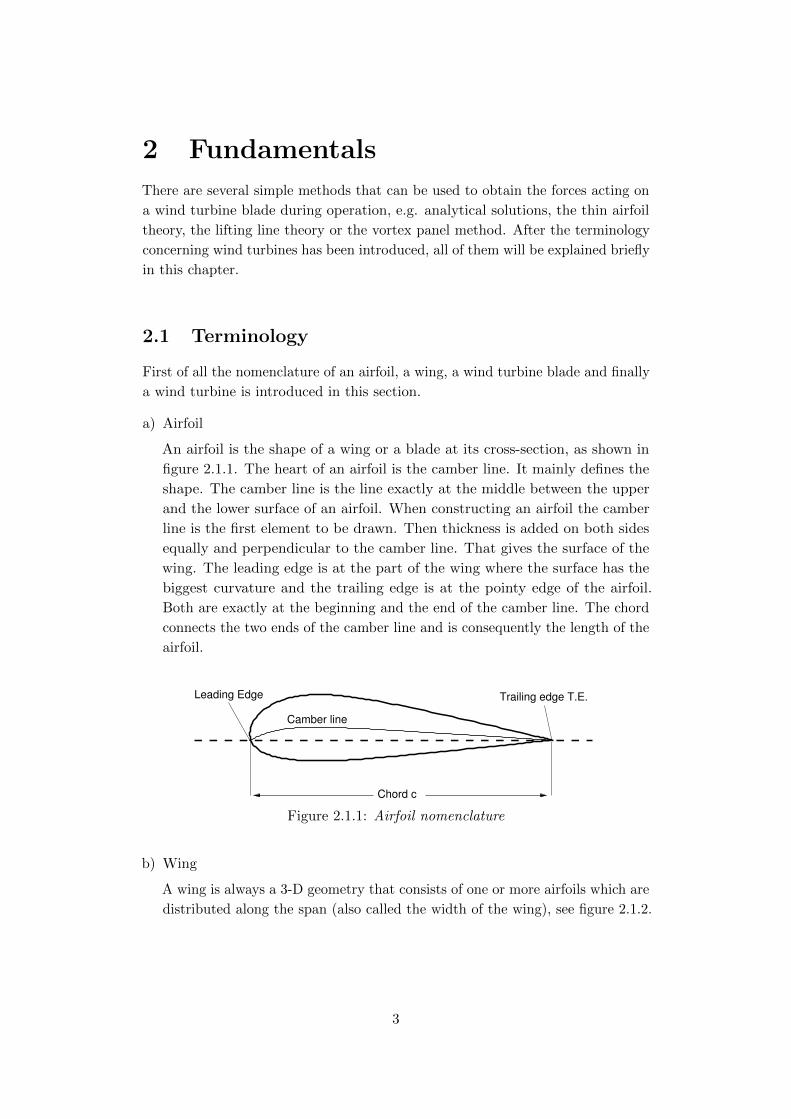
a) Airfoil
An airfoil is the shape of a wing or a blade at its cross-section, as shown in
figure 2.1.1. The heart of an airfoil is the camber line. It mainly defines the
shape. The camber line is the line exactly at the middle between the upper
and the lower surface of an airfoil. When constructing an airfoil the camber
line is the first element to be drawn. Then thickness is added on both sides
equally and perpendicular to the camber line. That gives the surface of the
wing. The leading edge is at the part of the wing where the surface has the
biggest curvature and the trailing edge is at the pointy edge of the airfoil.
Both are exactly at the beginning and the end of the camber line. The chord
connects the two ends of the camber line and is consequently the length of the
airfoil.
Camber line
Leading Edge
Chord c
Trailing edge T.E.
Figure 2.1.1: Airfoil nomenclature
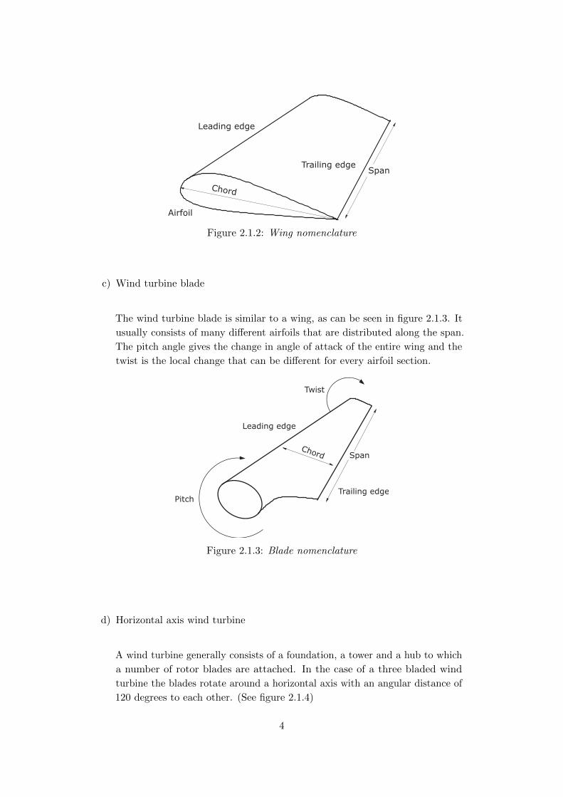
b) Wing
A wing is always a 3-D geometry that consists of one or more airfoils which are
distributed along the span (also called the width of the wing), see figure 2.1.2.
3
Chord
Leading edge
Trailing edgeSpan
Airfoil
Figure 2.1.2: Wing nomenclature
c) Wind turbine blade
The wind turbine blade is similar to a wing, as can be seen in figure 2.1.3. It
usually consists of many different airfoils that are distributed along the span.
The pitch angle gives the change in angle of attack of the entire wing and the
twist is the local change that can be different for every airfoil section.
Leading edge
Pitch
Chord Span
Twist
Trailing edge
Figure 2.1.3: Blade nomenclature
d) Horizontal axis wind turbine
A wind turbine generally consists of a foundation, a tower and a hub to which
a number of rotor blades are attached. In the case of a three bladed wind
turbine the blades rotate around a horizontal axis with an angular distance of
120 degrees to each other. (See figure 2.1.4)
4

Diameter
Tower
Foundation
Rotor blade
Hub height
Figure 2.1.4: Wind turbine nomenclature
2.2 Lift
In order to analyse the behaviour of a solid body in a free stream it is important
to know the surface force that it experiences due to the flow. As shown in
figure 2.2.1, the component of the force that is perpendicular to the free stream
is called lift, L, whereas the component in direction of the free stream is called
drag, D. To obtain the lift of an airfoil section or wing analytically, one has to
Drag
Lift
Free stream
Figure 2.2.1: Lift and Drag
know the density of air, ρ, the chord length, c, the free stream velocity, q∞ and
the lift coefficient, cL :
L =1
2ρ c q2
∞ cL (2.2.1)
5

2.3 Governing equations
For the calculation of a flow field around a solid body the main equations of fluid
flow theory have to be introduced. From the conservation of mass we get the
continuity equation∂ρu
∂x+∂ρv
∂y+∂ρw
∂z+∂ρ
∂t= 0 (2.3.1)
which can be reduced for an incompressible fluid (∂ρ∂t = 0, ∇ρ = 0):
∂u
∂x+∂v
∂y+∂w
∂z= ∇ · q = 0 (2.3.2)
The velocity potential, φ, can be used to express the velocity as the gradient of φ.
The velocity potential for irrotational flow can be applied to 3-D flows. Since it
can be obtained by differentiating in the same direction as the velocities
q = ∇φ (2.3.3)
we can write the velocity components as
u =∂φ
∂xv =
∂φ
∂yw =
∂φ
∂z(2.3.4)
The rotation of a fluid is given by ω = iωx + jωy + kωz and can be denoted as
the curl of q :
ω =1
2∇× q (2.3.5)
A useful tool to measure the rotation of a fluid element around itself as it moves
in the flow field is the vorticity, γ, that is defined to be twice the rotation.
γ = 2ω = ∇× q (2.3.6)
In contrast to the vorticity, the circulation, Γ, is not about the rotation of a fluid
element, but about the enclosing path of the fluid element. (Note: this does not
necessarily mean that the element moves on a circle.) Γ is the line integral of
velocity around a closed curve in the flow,[9].
Γ =
∮cq · dl =
∫∫S∇× q · n dS =
∫∫Sγ · n dS (2.3.7)
Furthermore the circulation is an important definition to calculate the lift of an
airfoil. According to the Kutta-Joukowski theorem, lift is directly proportional to
the circulation around a body
L′ = ρ q∞ Γ (2.3.8)
where L′, ρ, q∞ are lift per span, air density and free stream velocity, respectively.
Lift force acts always perpendicular to the free stream velocity and the vector
notation gives:
F = ρq× Γ (2.3.9)
6
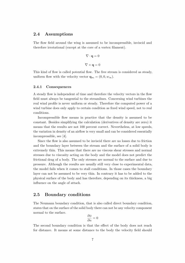
2.4 Assumptions
The flow field around the wing is assumed to be incompressible, inviscid and
therefore irrotational (except at the core of a vortex filament).
∇ · q = 0
∇× q = 0
This kind of flow is called potential flow. The free stream is considered as steady,
uniform flow with the velocity vector q∞ = (0, 0, w∞).
2.4.1 Consequences
A steady flow is independent of time and therefore the velocity vectors in the flow
field must always be tangential to the streamlines. Concerning wind turbines the
real wind profile is never uniform or steady. Therefore the computed power of a
wind turbine does only apply to certain condition as fixed wind speed, not to real
conditions.
Incompressible flow means in practice that the density is assumed to be
constant. Besides simplifying the calculation (derivatives of density are zero) it
means that the results are not 100 percent correct. Nevertheless, at low speeds,
the variation in density of an airflow is very small and can be considered essentially
incompressible, see [4].
Since the flow is also assumed to be inviscid there are no losses due to friction
and the boundary layer between the stream and the surface of a solid body is
extremely thin. This means that there are no viscous shear stresses and normal
stresses due to viscosity acting on the body and the model does not predict the
frictional drag of a body. The only stresses are normal to the surface and due to
pressure. Although the results are usually still very close to experimental data,
the model fails when it comes to stall conditions. In those cases the boundary
layer can not be assumed to be very thin. In contrary it has to be added to the
physical surface of the body and has therefore, depending on its thickness, a big
influence on the angle of attack.
2.5 Boundary conditions
The Neumann boundary condition, that is also called direct boundary condition,
states that on the surface of the solid body there can not be any velocity component
normal to the surface.∂φ
∂n= 0
The second boundary condition is that the effect of the body does not reach
for distance. It means at some distance to the body the velocity field should
7

be similar to the free stream upstream of the body. For an uniform free stream
follows:
limr→∞
∇φp = 0
where φp is the perturbation potential, respectively.
2.6 A vortex filament
A vortex filament is line of concentrated vorticity that induces a flow or velocity
everywhere in its neighbourhood, depending on the the distance to the filament.
dl
P
vorticity (gamma)
induced velocity
distance r
vortex filament
Figure 2.6.1: Induction by a vortex filament
Therefore the induced velocity qθ is
qθ =C
r(2.6.1)
where C is a constant and r is the distance from the vortex filament, respectively.
Using equation 2.3.7 and applying it to a vortex filament gives
Γ =
∮C
q · dl = qθ · 2πr (2.6.2)
Therefore the rotational velocity of P is
qθ =Γ
2πr(2.6.3)
The Helmholtz vortex theorem states that the strength of a vortex filament is
constant along its length and that it cannot end within a fluid. That means it
has to form a closed loop, as expressed by the circle integral.
8
Furthermore Kelvin’s circulation theorem declares that the circulation around a
closed curve formed by a set of contiguous fluid elements remains constant as the
fluid elements move. [2]
DΓ
Dt= 0 (2.6.4)
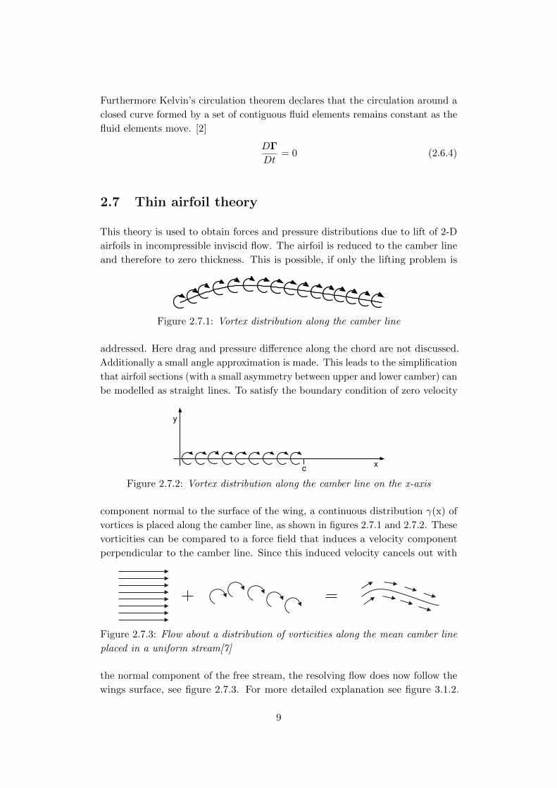
2.7 Thin airfoil theory
This theory is used to obtain forces and pressure distributions due to lift of 2-D
airfoils in incompressible inviscid flow. The airfoil is reduced to the camber line
and therefore to zero thickness. This is possible, if only the lifting problem is
Figure 2.7.1: Vortex distribution along the camber line
addressed. Here drag and pressure difference along the chord are not discussed.
Additionally a small angle approximation is made. This leads to the simplification
that airfoil sections (with a small asymmetry between upper and lower camber) can
be modelled as straight lines. To satisfy the boundary condition of zero velocity
x
y
c
Figure 2.7.2: Vortex distribution along the camber line on the x-axis
component normal to the surface of the wing, a continuous distribution γ(x) of
vortices is placed along the camber line, as shown in figures 2.7.1 and 2.7.2. These
vorticities can be compared to a force field that induces a velocity component
perpendicular to the camber line. Since this induced velocity cancels out with
Figure 2.7.3: Flow about a distribution of vorticities along the mean camber line
placed in a uniform stream[7]
the normal component of the free stream, the resolving flow does now follow the
wings surface, see figure 2.7.3. For more detailed explanation see figure 3.1.2.
9

The distribution of the vorticities can be used to obtain the lift per span L′:
L′ = ρ q∞
∫γ(x) dx (2.7.1)
2.8 Lifting surface method
In order to obtain the lift of a finite wing at a given angle of attack and free
stream velocity, the model of a lifting line can be used. This method uses vortex
filaments to model the influence of the body and the wake on the free stream.
Therefore a bound vortex is placed at 14 of the cord behind the leading edge
along the span of the wing. Additionally two trailing vortices starting at both
ends of the bound vortex and leaving the wing in chord wise direction simulate
the wake behind the wing (see figure 2.8.1). The wake is the region downstream
of an object in a free stream that differs from the free stream. It is caused by the
stream flowing around the object. Trailing vortices are mostly caused by pressure
differences. On both ends of a wing the higher pressure zone that is built under
the wing meets the lower pressure side from above the wing. That difference leads
to trailing vortices and therefore a wake roll-up. Together they form a so called
Bound vortex
Trailing votrices
Starting vortex
Figure 2.8.1: Horseshoe model for finite wing
”horseshoe vortex” of constant strength, Γ. Although the original theory states
that vortices can only exist in closed loop, the influence of the part connecting
the two trailing vortices, the starting vortex, can be neglected, see figure 2.8.2.
That is only possible for steady state conditions, where the starting vortex has
already moved very far downstream. Lift therefore is obtained as:
L = ρ b q∞ Γ (2.8.1)
Where ρ is the density of the fluid, b the span length, q∞ the free stream velocity
and Γ the strength for the bound vortex. Since the results of a single horseshoe
vortex do only represent a model for 2-D airfoil sections, it is mandatory to divide
the lifting line in many small bound vortices to obtain results that are valid for
3-D wings, as shown in figure 2.8.2. This method was first introduced by Ludwig
Pradtl and is therefore called ”Prandtl’s lifting line method” [9]. Trailing vortices
10
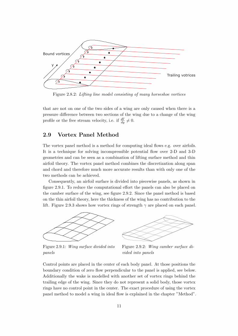
Trailing votrices
Bound vortices
y
Figure 2.8.2: Lifting line model consisting of many horseshoe vortices
that are not on one of the two sides of a wing are only caused when there is a
pressure difference between two sections of the wing due to a change of the wing
profile or the free stream velocity, i.e. if dΓdy 6= 0.
2.9 Vortex Panel Method
The vortex panel method is a method for computing ideal flows e.g. over airfoils.
It is a technique for solving incompressible potential flow over 2-D and 3-D
geometries and can be seen as a combination of lifting surface method and thin
airfoil theory. The vortex panel method combines the discretization along span
and chord and therefore much more accurate results than with only one of the
two methods can be achieved.
Consequently, an airfoil surface is divided into piecewise panels, as shown in
figure 2.9.1. To reduce the computational effort the panels can also be placed on
the camber surface of the wing, see figure 2.9.2. Since the panel method is based
on the thin airfoil theory, here the thickness of the wing has no contribution to the
lift. Figure 2.9.3 shows how vortex rings of strength γ are placed on each panel.
Figure 2.9.1: Wing surface divided into
panels
Figure 2.9.2: Wing camber surface di-
vided into panels
Control points are placed in the center of each body panel. At those positions the
boundary condition of zero flow perpendicular to the panel is applied, see below.
Additionally the wake is modelled with another set of vortex rings behind the
trailing edge of the wing. Since they do not represent a solid body, those vortex
rings have no control point in the center. The exact procedure of using the vortex
panel method to model a wing in ideal flow is explained in the chapter ”Method”.
11

Wing vortices
Wake vortices
Control point
Figure 2.9.3: Vortex ring on a flat wing and its wake
2.10 Induced velocity
To determine the actual forces on wind turbine blades it is mandatory to know
the exact velocity vectors of the flow field. Therefore it is necessary to know the
real angle of attack. It consists of the geometric angle of attack and the induced
angle. The induced angle can be obtained using the velocity component induced
by the wake.
The induced velocity or down-wash velocity, qi, is the velocity produced by
the wake behind the wing. Depending on the wake shape it has a larger or smaller
effect on the angle of attack. Since the lift of a wing is proportional to the angle
of attack it is mandatory to use the exact/real angle of attack: the effective angle
of attack αeff . It can be obtained by subtracting the induced from the geometric
angle of attack.
αeff = αgeo − αi (2.10.1)
Figure 2.10.1 shows the nomenclature of the introduced angles. Assuming a
effective velocity
free stream velocity
induced angle
effective angle
induced velocity
geometric angle
chordline
Figure 2.10.1: Angle of attack nomenclature
horizontal free stream velocity the induced velocity is pointing mainly downwards,
which is the reason for its name ”down-wash velocity”[5]. This velocity decreases
the real angle of attack as shown in figure 2.10.1.
Furthermore the lift, which is always perpendicular to the effective velocity,
12

does not point straight up, but slightly in the direction of the free stream velocity.
Therefore the lift in vertical direction is reduced and the drag is increased (see
figure 2.10.2).
lift perpendicular to effective velocity
induced drag
theoretical lift
effective velocity
free stream velocity
to the free stream
lift component perpendicular
induced velocity
Figure 2.10.2: Decreased lift due to induced velocities
Especially the analytical solution for lift depends on the exact (effective) angle of
attack:
2D-airfoil:
Using equation2.2.1 and substituting cL with 2πα we get
L = αeff π ρ c q2∞ (2.10.2)
where c is the chord length of the wing and q∞ the free stream velocity.
3-D wing:
L = α2eff π ρ c q∞
2 AR
AR+ 2(2.10.3)
Where AR is the aspect ratio of the wing and can be obtained as:
AR =span2
area of airfoil section(2.10.4)
For a rectangular planform that would be:
AR =b2
c · b=b
c(2.10.5)
where b is the span length and c the chord length of a wing.
13

3 Method
3.1 Vortex panel method - step by step
First of all, as mentioned in section 2.9, the camber surface has to be divided
into panels. Then vortex rings and control points are placed on each panel. An
example of a vortex panel is given in figure 3.1.1. A closed vortex ring of constant
strength γ and a control point are placed on the panel. The direction of the
circulation follows the right-hand rule. Those vortex rings are used to model
circulation (gamma)
vortex ring
control point
bound vortex
panel
panel lenght l
panel width b
Figure 3.1.1: Vortex panel nomenclature
the wings physical surface. All vortex rings induce a velocity component at the
control point in the center of each vortex ring. Here, the Neumann boundary
condition of zero velocity component normal to the surface is applied. Therefore
the following equations result:
qeff = q∞ + qi (3.1.1)
qi = qeff − q∞ (3.1.2)
As shown in figure 3.1.2 an induced velocity qi has to be added to the free stream
velocity q∞ in order to gain an effective velocity qeff that is purely parallel to
the wings surface. Therefore the vortex panel method is based on the calculation
of the of the induced velocities at the control points. For the velocity induced by
a vortex filament holds:
dqi =γ
4π
dl× r
| r |3(3.1.3)
Equation 3.1.3 is derived from the Biot-Savart Law and shows that the induced
velocity depends on the strength of the vortex filament and its distance r. [9]
14

induced velocity
resulting velocity
free stream velocity
wing panel
vortex ring
Figure 3.1.2: Vector summation on a vortex panel in a free stream
Hence the induced velocity is given by the integral along the whole vortex ring.
qi =γ
4π
∫c
r× dl| r |3
(3.1.4)
Since the vortex rings are quadratic elements, the easiest way to get qi is to
calculate the induced velocity of each vortex filament separately. Given that a
vorticity (gamma)
vortex filament
control point
rarb
a
b
Figure 3.1.3: Local vectors ra and rb from a control point to an arbitrary vortex
filament
and b are start- and endpoints on a filament and ra and rb are the vectors from
the control point to a and b, see figure 3.1.3, the following equation results:
q1 =γ
4π
(ra + rb)(ra × rb)
rarb(rarb + ra · rb)(3.1.5)
Repeating this procedure for the remaining three filaments, we consequently get
q2, q3 and q4. qi can therefore be obtained with
qi = q1 + q2 + q3 + q4 (3.1.6)
As a simple example of how the vortex panel method is applied to a wing, a 3-D
symmetric wing at an arbitrary angle of attack α is used. The wing is divided
into nine vortex panels as can be seen in figure 3.1.4. Additionally there are six
wake panels shown in the figure. The grid nodes are numbered with j as a counter
15

1
1i3
2
1
2
3
k2
Wake vortices
Wing vortices
Control point
j
Figure 3.1.4: Vortex panels distributed on the camber surface of a symmetric wing
along the span of the wing, i as a counter along the camber line and k from the
trailing edge of the wing to the end of the wake.
Calculating the induced velocities for γ = 1, the influence coefficients ai can
be obtained. They represent the influence of every vortex ring of wing and wake
to each control point, as figure 3.1.5 shows for one control point.
ai = qi(γ = 1) (3.1.7)
1
1i3
2
1
2
3
k2
Wake vortices
Wing vortices
j
Figure 3.1.5: Influence of the vortex rings on a control point
Using the Neumann boundary condition, the following equation for a solid body
in a uniform flow field can be obtained
∂(φb + φ∞)
∂n= 0 (3.1.8)
and therefore
∇(φb + φ∞) · n = 0 (3.1.9)
or
(qi + q∞) · n = 0 (3.1.10)
This means that the normal component of the free stream velocity, q∞ · n, and
the normal component of the induced velocity, qi · n, have to have the opposite
magnitude in order to cancel each other out. The free stream velocity can be
moved to the right-hand side of the equation:
qi · n = −q∞ · n (3.1.11)
16

The induced velocity at one control point consists of the influence coefficients and
the vortex strengths of all blade and wake vortex rings,
qi1 = ain γn (3.1.12)
where n is the number of vortex rings ((j − 1)(i + k + 2)). Substituting equa-
tion 3.1.12 into equation 3.1.11 we get
ain n · γn = −q∞1n (3.1.13)
Expanding the equation for all control points (the total number of control points
is m ((j − 1)(i+ 1))) all influence coefficients can be stored in the matrix Aim,n.
Aim,n =
a1,1 a1,2 · · · a1,n
a2,1 a2,2 · · · a2,n
......
. . ....
am,1 am,2 · · · am,n
(3.1.14)
qi m,n = Aim,n γn (3.1.15)
With equation 3.1.15 the solution equation can be rewritten as:
Aim,n n · γn = −q∞m · n (3.1.16)
a1,1 a1,2 · · · a1,n
a2,1 a2,2 · · · a2,n
......
. . ....
am,1 am,2 · · · am,n
γ1
γ2
...
γn
= −
q∞,1q∞,2
...
q∞,m
(3.1.17)
This gives a set of linear equations that can not be solved for all γ of body and
wake because there are still to many unknowns. Equation 3.1.17 contains only
the equations for the body γ but the wake and body depend on each other. That
problem is solved using the Kutta condition.
The Kutta condition applies to the vortex panel method, the thin airfoil theory
as well as the lifting line theory. It manly states that the flow should leave the
trailing edge of a wing smoothly. To satisfy that condition the vorticity γ at the
trailing edge T.E. has to be zero.
γT.E. = 0 (3.1.18)
For the vortex panel method this is applied by setting the strength of the first
wake vortex ring equal to the strength of the last vortex ring on the wing. That
way they will always cancel out at the trailing edge. Therefore, for each wake
vortex ring, an equation is added that states that the strength is the same as the
one of the wing panel at the trailing edge. Now the set of equations can be solved
17

for all γ. With the obtained values of the circulation and equation 2.3.8 forces on
the wing can be calculated.
In order to apply the vortex panel method to a wind turbine important changes
have to be made. A wind turbine is a rotating system with a non-homogeneous
velocity distribution along the turbine blades. Therefore the free stream velocity
is now substituted by the vector addition of the free stream velocity and the
rotational velocity. Effects of fictitious forces as the centrifugal and Coriolis force
are neglected here.
q∞+rot = q∞ + qrot (3.1.19)
Furthermore most wind turbines have more than one blade. The NREL 5MW
wind turbine has 3 blades of the same kind. This means that the wake behind
a wind turbine, that was shed by blade one, does not only affect blade one, but
also blades two and three and vice versa. Additionally the blades affect each
other. In order to get the correct induced velocities for every control point on
each blade all vortex rings of all blades and their wakes have to be included in the
solution matrix. Then induced velocities can be calculated by using the influence
coefficients of all wake vortex rings and their calculated strengths.
With the equation for the effective velocity 3.1.1 and the Kutta-Joukowski
theorem the forces on the rotor blade can be calculated for every control point:
F = ρ · qeff × Γ (3.1.20)
where Γ is the difference in vortex strength of each vortex ring and its neighbour
in direction to the leading edge.
Γn = γn − γn−1 (3.1.21)
Since the first panel at the leading edge has no neighbour in downstream direction
the value of Γn is equal to its vortex strength γn.
In this thesis two forces are differentiated: the force normal to the rotor plane
(usually in free stream direction) Fnor and the force tangential to the rotor plane
(in rotational direction) Ftang, see figure 3.1.6.
18

tangential force
normal force
Figure 3.1.6: Normal and tangential forces with respect to the rotor plane
3.2 Implementation in MATLAB
The vortex panel method was implemented in MATLAB as shown in figure 3.2.1.
First of all a geometry has to be loaded from file or in case of a symmetric wing,
the four corners of the wing have to be assigned. Then important parameters
such as grid size, wake length and the maximal residual have to be set. Now a
grid can be generated on the wings/blades camber surface. Then the initial shape
of the wake is prescribed.
Furthermore control points are set in the center of each wing vortex ring. At
these points the condition of zero velocity component normal to the surface is
applied later on in the code. Therefore normal vectors have to be obtained at
every control point.
The next steps have to be within the iteration loop since the values of the
parameters, especially the ones connected to the wake, can change with every
iteration. With the information about the position of the blade and wake vortices
the influence coefficients can be obtained and gathered in the matrix Ai. For
each control point on the wing and each node in the wake grid the influence of
all vortex rings is taken into account. The normal component of these influence
coefficients multiplied by the strength of each vortex ring gives the left-hand side
(lhs) of the equation:
Ai · n γ = −q∞+rot · n (3.2.1)
The right-hand side (rhs) is obtained by deriving the normal component of the
free stream and rotational velocity at each control point.
Then the equation is solved for the vorticity vector γ, which is the key point
of the code. With the vortex strengths, the effective and induced velocities are
19

found quickly.
qi = Ai · γ (3.2.2)
Knowing those it is now possible to calculate the new position of the wake
(depending on the chosen wake shape, see section 3.3.2). These actions are
repeated till the position of the wake does not change any more, according to the
accepted residual.
Now the pressure distribution, lift, normal and tangential forces can be calcu-
lated and plotted.
load geometry and set parameters
grid and initial wake geometry generation
placement of control points in the middle of body panels
normal vector to each control point
lhs: influence coefficients times gamma
rhs: normal component of free stream velocity
solve for gamma
Induced and effective velocities
new position of wake
new wake = old wake?
lift, normal and tangential forces
plot
No
Yes
updated or free wake?No
Yes
Figure 3.2.1: Implementation in MATLAB
20
3.3 Model used in MATLAB simulation
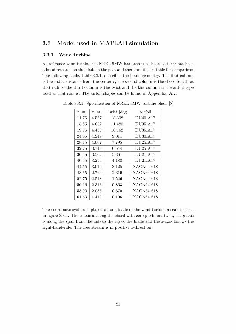
3.3.1 Wind turbine
As reference wind turbine the NREL 5MW has been used because there has been
a lot of research on the blade in the past and therefore it is suitable for comparison.
The following table, table 3.3.1, describes the blade geometry. The first column
is the radial distance from the center r, the second column is the chord length at
that radius, the third column is the twist and the last column is the airfoil type
used at that radius. The airfoil shapes can be found in Appendix. A.2.
Table 3.3.1: Specification of NREL 5MW turbine blade [8]
r [m] c [m] Twist [deg] Airfoil
11.75 4.557 13.308 DU40 A17
15.85 4.652 11.480 DU35 A17
19.95 4.458 10.162 DU35 A17
24.05 4.249 9.011 DU30 A17
28.15 4.007 7.795 DU25 A17
32.25 3.748 6.544 DU25 A17
36.35 3.502 5.361 DU21 A17
40.45 3.256 4.188 DU21 A17
44.55 3.010 3.125 NACA64 618
48.65 2.764 2.319 NACA64 618
52.75 2.518 1.526 NACA64 618
56.16 2.313 0.863 NACA64 618
58.90 2.086 0.370 NACA64 618
61.63 1.419 0.106 NACA64 618
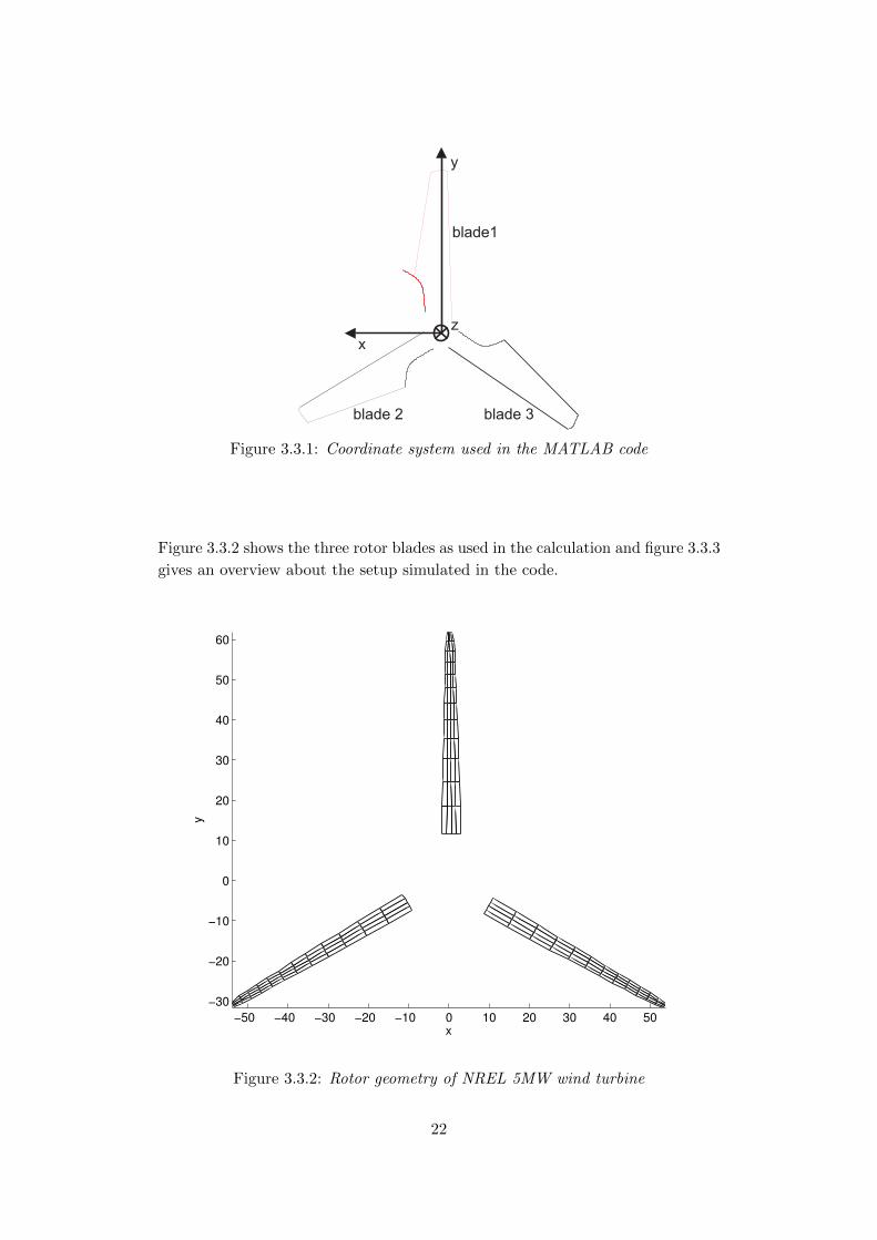
The coordinate system is placed on one blade of the wind turbine as can be seen
in figure 3.3.1. The x-axis is along the chord with zero pitch and twist, the y-axis
is along the span from the hub to the tip of the blade and the z-axis follows the
right-hand-rule. The free stream is in positive z-direction.
21
x
y
z
blade 2 blade 3
blade1
Figure 3.3.1: Coordinate system used in the MATLAB code
Figure 3.3.2 shows the three rotor blades as used in the calculation and figure 3.3.3
gives an overview about the setup simulated in the code.
−50 −40 −30 −20 −10 0 10 20 30 40 50
−30
−20
−10
0
10
20
30
40
50
60
x
y
Figure 3.3.2: Rotor geometry of NREL 5MW wind turbine
22
Radius
63 m
Hub height
90m
Free stream
1) 8 m/s
2) 11.4 m/s
Rotational velocity
2) 12.1 rpm
1) 9.6 rpm
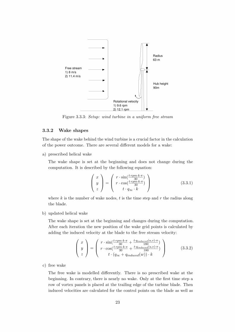
Figure 3.3.3: Setup: wind turbine in a uniform free stream
3.3.2 Wake shapes
The shape of the wake behind the wind turbine is a crucial factor in the calculation
of the power outcome. There are several different models for a wake:
a) prescribed helical wake
The wake shape is set at the beginning and does not change during the
computation. It is described by the following equation: x
y
z
=
r · sin( t·rpm·k·π30 )
r · cos( t·rpm·k·π30 )
t · q∞ · k
(3.3.1)
where k is the number of wake nodes, t is the time step and r the radius along
the blade.
b) updated helical wake
The wake shape is set at the beginning and changes during the computation.
After each iteration the new position of the wake grid points is calculated by
adding the induced velocity at the blade to the free stream velocity: x
y
z
=
r · sin( t·rpm·k·π30 + t·qinduced(u,v)·π180 )
r · cos( t·rpm·k·π30 + t·qinduced(u,v)·π180 )
t · (q∞ + qinduced(w)) · k
(3.3.2)
c) free wake
The free wake is modelled differently. There is no prescribed wake at the
beginning. In contrary, there is nearly no wake. Only at the first time step a
row of vortex panels is placed at the trailing edge of the turbine blade. Then
induced velocities are calculated for the control points on the blade as well as
23

the grid point of the wake. With the information of the induced velocity and
the free stream velocity at all wake grid points, they can be moved according
to the combined velocity vectors. That way the wake moves freely behind the
wind turbine.
24
4 Results
In this chapter the results of the above introduced methods applied on three
different cases are discussed. The first case is a 3-D wing. That means that the
results are valid for a wing with a finite wing span. A single turbine blade that
is rotating around a horizontal axis formulates the second case and a full scale
wind turbine with three blades is used in case three. Furthermore these results
are validated using GENUVP, CFD and BEM data.
4.1 3-D wing
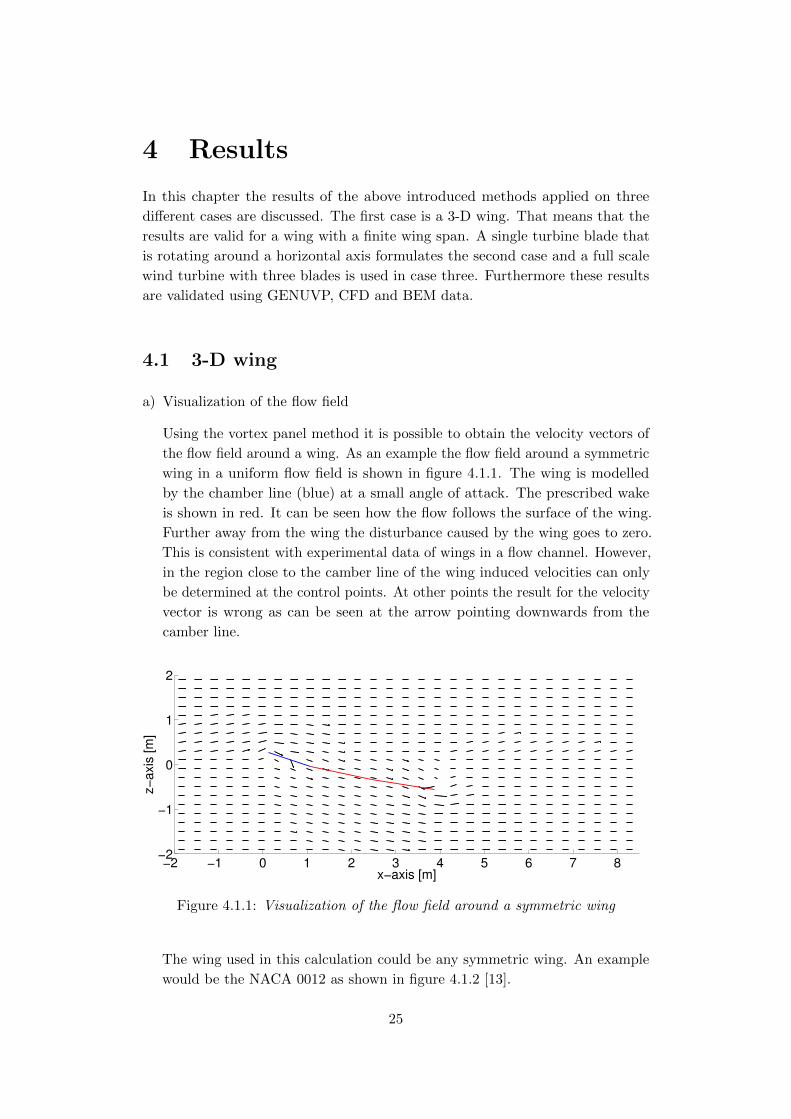
a) Visualization of the flow field
Using the vortex panel method it is possible to obtain the velocity vectors of
the flow field around a wing. As an example the flow field around a symmetric
wing in a uniform flow field is shown in figure 4.1.1. The wing is modelled
by the chamber line (blue) at a small angle of attack. The prescribed wake
is shown in red. It can be seen how the flow follows the surface of the wing.
Further away from the wing the disturbance caused by the wing goes to zero.
This is consistent with experimental data of wings in a flow channel. However,
in the region close to the camber line of the wing induced velocities can only
be determined at the control points. At other points the result for the velocity
vector is wrong as can be seen at the arrow pointing downwards from the
camber line.
−2 −1 0 1 2 3 4 5 6 7 8−2
−1
0
1
2
x−axis [m]
z−
axis
[m
]
Figure 4.1.1: Visualization of the flow field around a symmetric wing
The wing used in this calculation could be any symmetric wing. An example
would be the NACA 0012 as shown in figure 4.1.2 [13].
25
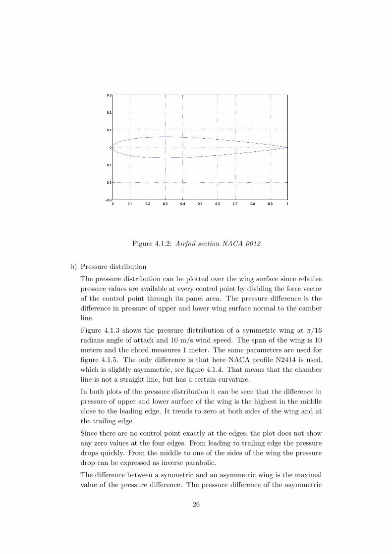
Figure 4.1.2: Airfoil section NACA 0012
b) Pressure distribution
The pressure distribution can be plotted over the wing surface since relative
pressure values are available at every control point by dividing the force vector
of the control point through its panel area. The pressure difference is the
difference in pressure of upper and lower wing surface normal to the camber
line.
Figure 4.1.3 shows the pressure distribution of a symmetric wing at π/16
radians angle of attack and 10 m/s wind speed. The span of the wing is 10
meters and the chord measures 1 meter. The same parameters are used for
figure 4.1.5. The only difference is that here NACA profile N2414 is used,
which is slightly asymmetric, see figure 4.1.4. That means that the chamber
line is not a straight line, but has a certain curvature.
In both plots of the pressure distribution it can be seen that the difference in
pressure of upper and lower surface of the wing is the highest in the middle
close to the leading edge. It trends to zero at both sides of the wing and at
the trailing edge.
Since there are no control point exactly at the edges, the plot does not show
any zero values at the four edges. From leading to trailing edge the pressure
drops quickly. From the middle to one of the sides of the wing the pressure
drop can be expressed as inverse parabolic.
The difference between a symmetric and an asymmetric wing is the maximal
value of the pressure difference. The pressure difference of the asymmetric
26

wing is more equally distributed and has therefore a smaller maximum. This
can be explained with the smoother flow guidance of the bent camber line.
0.2 0.4 0.6 0.82
4
6
8
0.2
0.4
0.6
0.8
1
1.2
1.4
1.6
1.8
2
2.2
span [m]
chord [m]
Pre
ssure
[N
/m2] x 1
02
0
0.5
1
1.5
2
2.5
Figure 4.1.3: Pressure distribution, symmetric wing
Figure 4.1.4: Airfoil section NACA 2414
27
0.2 0.4 0.6 0.8
2
4
6
8
0.2
0.4
0.6
0.8
1
1.2
1.4
1.6
1.8
span [m]
chord [m]
Pre
ssure
[N
/m2] x 1
02
0
0.5
1
1.5
2
2.5
Figure 4.1.5: Pressure distribution, asymmetric wing
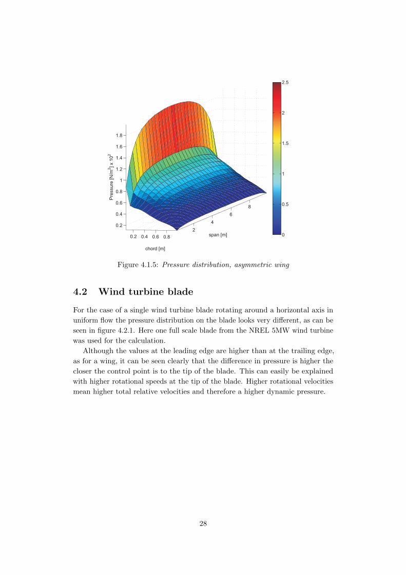
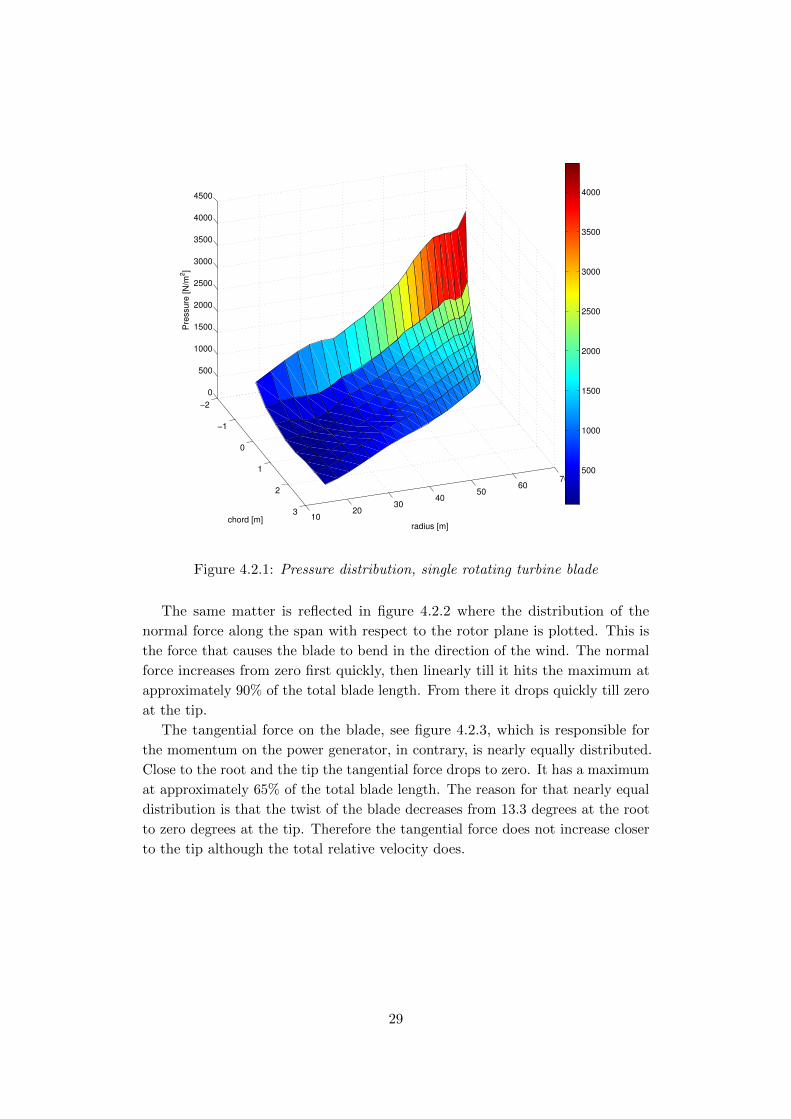
4.2 Wind turbine blade
For the case of a single wind turbine blade rotating around a horizontal axis in
uniform flow the pressure distribution on the blade looks very different, as can be
seen in figure 4.2.1. Here one full scale blade from the NREL 5MW wind turbine
was used for the calculation.
Although the values at the leading edge are higher than at the trailing edge,
as for a wing, it can be seen clearly that the difference in pressure is higher the
closer the control point is to the tip of the blade. This can easily be explained
with higher rotational speeds at the tip of the blade. Higher rotational velocities
mean higher total relative velocities and therefore a higher dynamic pressure.
28
−2
−1
0
1
2
310
2030
4050
6070
0
500
1000
1500
2000
2500
3000
3500
4000
4500
radius [m]chord [m]
Pre
ssure
[N
/m2]
500
1000
1500
2000
2500
3000
3500
4000
Figure 4.2.1: Pressure distribution, single rotating turbine blade
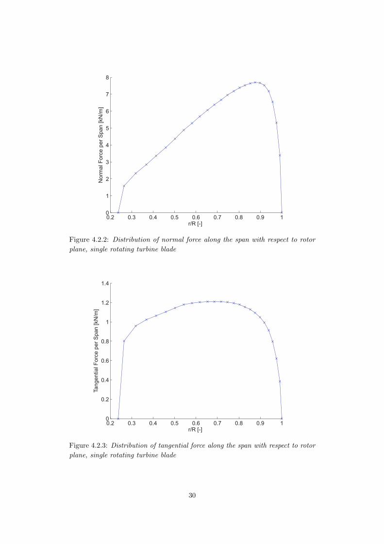
The same matter is reflected in figure 4.2.2 where the distribution of the
normal force along the span with respect to the rotor plane is plotted. This is
the force that causes the blade to bend in the direction of the wind. The normal
force increases from zero first quickly, then linearly till it hits the maximum at
approximately 90% of the total blade length. From there it drops quickly till zero
at the tip.
The tangential force on the blade, see figure 4.2.3, which is responsible for
the momentum on the power generator, in contrary, is nearly equally distributed.
Close to the root and the tip the tangential force drops to zero. It has a maximum
at approximately 65% of the total blade length. The reason for that nearly equal
distribution is that the twist of the blade decreases from 13.3 degrees at the root
to zero degrees at the tip. Therefore the tangential force does not increase closer
to the tip although the total relative velocity does.
29
0.2 0.3 0.4 0.5 0.6 0.7 0.8 0.9 10
1
2
3
4
5
6
7
8
r/R [-]
No
rma
l F
orc
e p
er
Sp
an
[kN
/m]
Figure 4.2.2: Distribution of normal force along the span with respect to rotor
plane, single rotating turbine blade
0.2 0.3 0.4 0.5 0.6 0.7 0.8 0.9 10
0.2
0.4
0.6
0.8
1
1.2
1.4
r/R [-]
Ta
ng
en
tia
l F
orc
e p
er
Sp
an
[kN
/m]
Figure 4.2.3: Distribution of tangential force along the span with respect to rotor
plane, single rotating turbine blade
30

4.3 Wind turbine NREL 5MW
4.3.1 Grid analysis
In order to be able to run many different cases for different methods it is mandatory
to find a grid size that is as fine as necessary but also as coarse as possible.
Therefore the grid size of the panels on the blade (i, j) and the wake (k, j) as
well as the wake length have been investigated. For the analysis a basic set of
parameters was chosen, see table. 4.3.1. For each investigation all parameters
are according to the table except for the investigated one. That parameter was
varied from its maximum or a very high value till the smallest possible value.
To capture the difference that is caused by the change of the parameter a
power ratio was chosen. This ratio consists of the calculated power outcome for
the specific set of parameters divided by the power outcome of the investigated
parameter at the highest value. Regarding the grid counter along the camber
Table 4.3.1: Basic set of parameters for grid analysis
Symbol Description Value
i grid counter along camber line 5
j grid counter from root to tip 9
k grid counter from trailing edge till end of wake 18
w wake length in rotations 1
q∞ free stream velocity in meters per second 8
ω rotational velocity in rad per second 1.0032
1 2 3 4 5 6 7 8 9 100.5
0.6
0.7
0.8
0.9
1
1.1
i [−]
po
we
r ra
tio
[−
]
change in power
1% range
chosen i
Figure 4.3.1: Change of power due to a change of the grid size in chordwise
direction
31

line, i, it can be seen in fig 4.3.1 that the power ratio drops quickly when i
becomes coarser. The red lines stand for the 1% range of the power ratio for
the highest value of i. To stay in between the two lines i equals nine has to be
chosen. In figure 4.3.2 the grid number from root to tip was investigated. Here
0 5 10 15 20 250.2
0.3
0.4
0.5
0.6
0.7
0.8
0.9
1
1.1
j [−]
pow
er
ratio [−
]
change in power
1% range
smallest possible j
chosen j
7 13
Figure 4.3.2: Change of power due to a change of the grid size in radial direction
it can be seen that while decreasing j the power ratio stays in the 1% range till
j equals seven and drops quickly afterwards. Hence due to graphical problems
(recall: tangential and normal forces are plotted along the turbine blade from
root to tip) j equals 13 was chosen for further investigations.
0 1 2 3 4 5 60.9
1
1.1
1.2
1.3
1.4
number of rotations [−]
po
wer
ratio [
−]
change in power
2% range
chosen wake length
Figure 4.3.3: Change of power due to a change of wake length behind the wind
turbine
32
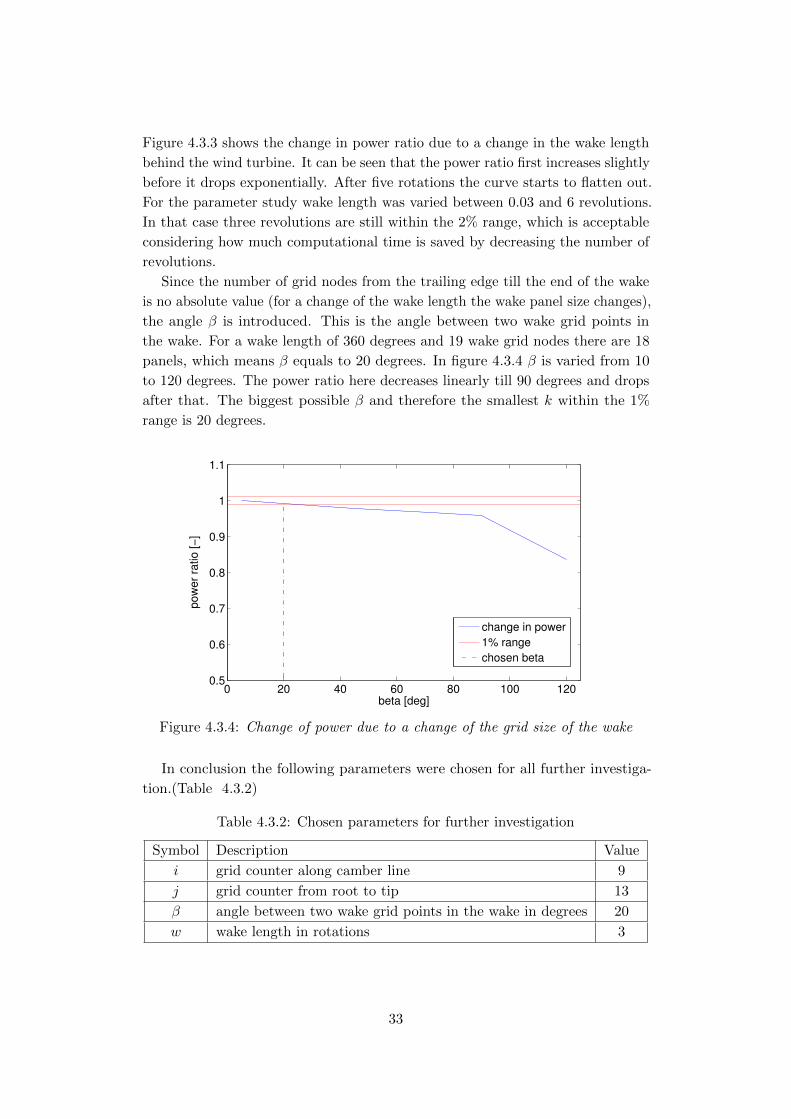
Figure 4.3.3 shows the change in power ratio due to a change in the wake length
behind the wind turbine. It can be seen that the power ratio first increases slightly
before it drops exponentially. After five rotations the curve starts to flatten out.
For the parameter study wake length was varied between 0.03 and 6 revolutions.
In that case three revolutions are still within the 2% range, which is acceptable
considering how much computational time is saved by decreasing the number of
revolutions.
Since the number of grid nodes from the trailing edge till the end of the wake
is no absolute value (for a change of the wake length the wake panel size changes),
the angle β is introduced. This is the angle between two wake grid points in
the wake. For a wake length of 360 degrees and 19 wake grid nodes there are 18
panels, which means β equals to 20 degrees. In figure 4.3.4 β is varied from 10
to 120 degrees. The power ratio here decreases linearly till 90 degrees and drops
after that. The biggest possible β and therefore the smallest k within the 1%
range is 20 degrees.
0 20 40 60 80 100 1200.5
0.6
0.7
0.8
0.9
1
1.1
beta [deg]
pow
er
ratio [−
]
change in power
1% range
chosen beta
Figure 4.3.4: Change of power due to a change of the grid size of the wake
In conclusion the following parameters were chosen for all further investiga-
tion.(Table 4.3.2)
Table 4.3.2: Chosen parameters for further investigation
Symbol Description Value
i grid counter along camber line 9
j grid counter from root to tip 13
β angle between two wake grid points in the wake in degrees 20
w wake length in rotations 3
33

4.3.2 Comparison of Vortex Panel Method (VPM), Reduced
Vortex Panel Method (RVPM) and Lifting Surface Method
In this section the vortex panel method (VPM) with a number of panels chordwise,
the reduced vortex panel method (RVPM) with one panel chordwise and the
lifting surface method are compared to each other. The induced velocity, the
effective angle of attack, the strength of vorticity γ, the normal and the tangential
force distribution are evaluated. Additionally two different wake shapes are used
for the computation, the prescribed helical wake and the updated helical wake.
Figure 4.3.5 shows the induced velocities along the blade from root to tip.
For the reduced vortex panel method and the lifting surface method the induced
velocities are the ones located at the control points since there is only one control
point in chordwise direction. In the lifting surface method the wake consist of
the trailing vortices and the vortex panel methods use vortex rings to model the
wake. Nevertheless, in steady-state condition the wake in VPM and RVPM is
similar to trailing vortices.
0.2 0.3 0.4 0.5 0.6 0.7 0.8 0.9 11
1.2
1.4
1.6
1.8
2
2.2
2.4
2.6
2.8
r/R [−]
win
du
ce
d [
m/s
]
vpm prescribed
vpm updated
rvpm prescribed
rvpm updated
lifting surface prescribed
lifting surface updated
Figure 4.3.5: Induced velocity distribution normal to rotor plane
The induced velocities of the vortex panel method are the average values of all
control points in one airfoil section. For the all vortex panel lines the induced
velocity increases from a value around 1.2 ms to 2.8 m
s (VPM) and 1.9 ms (RVPM).
The values of the lifting surface method in contrary decrease from between 1.9
and 2.0 ms to an minimum at 50% of the total blade length and increase again
approaching the values of the vortex panel method close to the tip. However, the
34

last data point at 98% of the total blade length resembles the reduced vortex
panel method. Moreover, it is obvious that the values of the updated wake are
consistently higher than the ones of the prescribed wake. Due to updating where
the wake includes the induced velocity, the wake is overall closer to the wind
turbine than for the prescribed wake. Therefore the impact on the blade in the
form of induced velocity is higher.
Since the induced velocity has a big impact on the angle of attack, the effective
angle of attack changed correspondingly. The red line in figure 4.3.6 is the
geometric angle off attack that is calculated from free stream and rotational
velocity. All lines with markers are effective angles of attack, that include the
effect of the induced velocity. As expected, those angles are much smaller than the
geometric angle of attack, especially where the induced velocity is high. Here, the
values of the updated wake are consistently lower than the ones of the prescribed
wake. The distributions of the strength of vorticity γ in figure 4.3.7 are very
0.2 0.3 0.4 0.5 0.6 0.7 0.8 0.9 14
5
6
7
8
9
10
11
12
13
r/R [−]
alp
ha
effective [
de
g]
Geometric
vpm prescribed
vpm updated
vpm 1panel prescribed
vpm 1panel updated
lifting surface prescribed
lifting surface updated
Figure 4.3.6: Effective angle of attack along the blade
similar at the tip of the turbine blade but the further to the root the more they
differ. From tip to root the values increase very quickly to values around 40 m2
s at
approximately 85% of the total blade length and decrease then to values between
30 and 40 m2
s . Here, the values of the updated wake are consistently lower than
the ones of the prescribed wake.
35

0.2 0.3 0.4 0.5 0.6 0.7 0.8 0.9 120
25
30
35
40
45
r/R [−]
circula
tion [m
2/s
]
vpm prescribed
vpm updated
rvpm prescribed
rvpm updated
lifting surface prescribed
lifting surface updated
Figure 4.3.7: Vortex distribution along the blade
0.2 0.3 0.4 0.5 0.6 0.7 0.8 0.9 1500
1000
1500
2000
2500
3000
3500
4000
4500
r/R [−]
norm
al fo
rce p
er
span [N
/m]
vpm prescribed
vpm updated
rvpm prescribed
rvpm updated
lifting surface prescribed
lifting surface updated
Figure 4.3.8: Normal velocity distribution along the blade
The results of the normal, figure 4.3.8, and tangential force, figure 4.3.9, are
similar to the results for a single turbine blade. The difference is the magnitude
36

of the values. It is smaller than for one turbine blade because those plots were
generated for higher wind speeds and there are now three blades in the same area
instead of one. Particularly conspicuous is that the values of the reduced vortex
panel method and lifting surface method are about 40% lower than the values of
the vortex panel method. That can be explained through the disregard of the
camber line curvature.
0.2 0.3 0.4 0.5 0.6 0.7 0.8 0.9 1100
150
200
250
300
350
400
450
500
r/R [−]
tangential fo
rce p
er
span [N
/m]
vpm prescribed
vpm updated
rvpm l prescribed
rvpm updated
lifting surface prescribed
lifting surface updated
Figure 4.3.9: Tangential velocity distribution along the blade
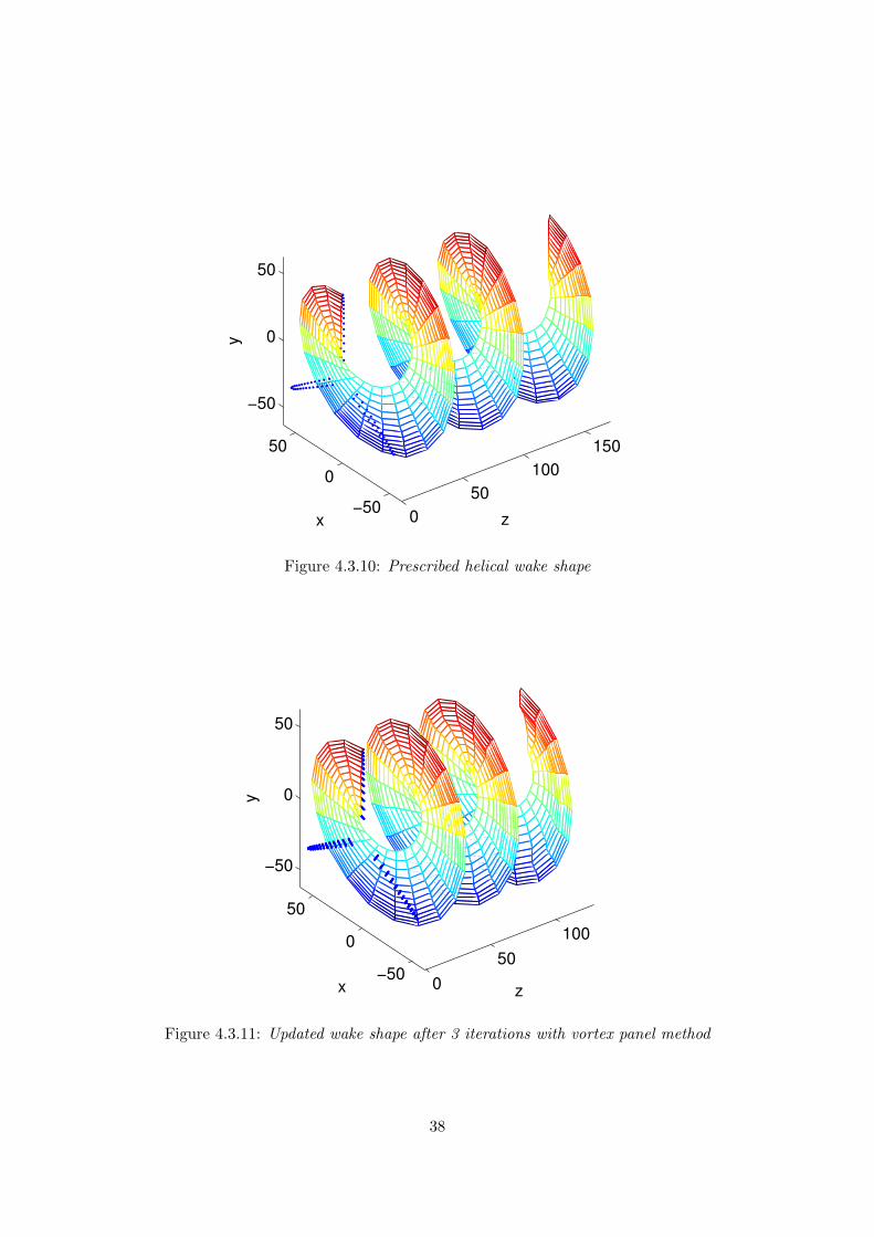
4.3.3 Wake shapes
In this section the wake behind the wind turbine is plotted for one turbine blade
only in order to increase clarity. The rotor plane is in the x− y-plane and the
turbine rotates clockwise, seen in positive z-direction. The free stream velocity is
in positive z-direction. Here three rotations of the turbine blade are plotted. In
figure 4.3.10 the prescribed helical wake is shown. It is a simple wake calculated
according to equation 3.3.1 with a total wake length of 170 m for three rotations.
For the updated wakes the wake shape was found in an iterative process till the
residual was smaller than 0.01. In these cases it required only three iterations. As
expected, the updated wake shapes are compressed compared to the prescribed
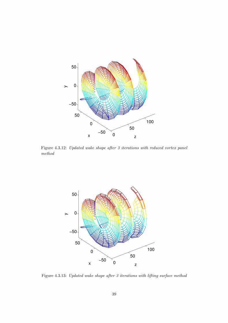
wake due to the addition of the the induced velocities (see figures 4.3.11, 4.3.12
and 4.3.13). The total wake length of the wake of the vortex panel method, the
reduced vortex panel method and the lifting surface method is between 126 and
130 m. The main difference between the three updated wakes is their shape along
the radius. All shapes are according to their induced velocity distribution in
figure 4.3.5.
37
0
50
100
150
−50
0
50
−50
0
50
zx
y
Figure 4.3.10: Prescribed helical wake shape
0
50
100
−50
0
50
−50
0
50
zx
y
Figure 4.3.11: Updated wake shape after 3 iterations with vortex panel method
38
0
50
100
−50
0
50
−50
0
50
zx
y
Figure 4.3.12: Updated wake shape after 3 iterations with reduced vortex panel
method
0
50
100
−50
0
50
−50
0
50
zx
y
Figure 4.3.13: Updated wake shape after 3 iterations with lifting surface method
39
4.4 Validation
To validate the results data from three different sources was investigated. Since
there was only data available for certain cases with different wind speeds and
rotational velocities, the validation section was split up in GENUVP and BEM &
CFD. GENUVP is an unsteady flow solver based on vortex blob approximations
developed for rotor systems by National Technical University of Athens (courtesy
of Prof. Spyros Voutsinas) [11]. GENUVP includes a dynamic stall model as well
as friction which is considered based on the Cd vs. α table [10]. In this section
the vortex panel methods with updated wake were used for all figures.
4.4.1 GENUVP
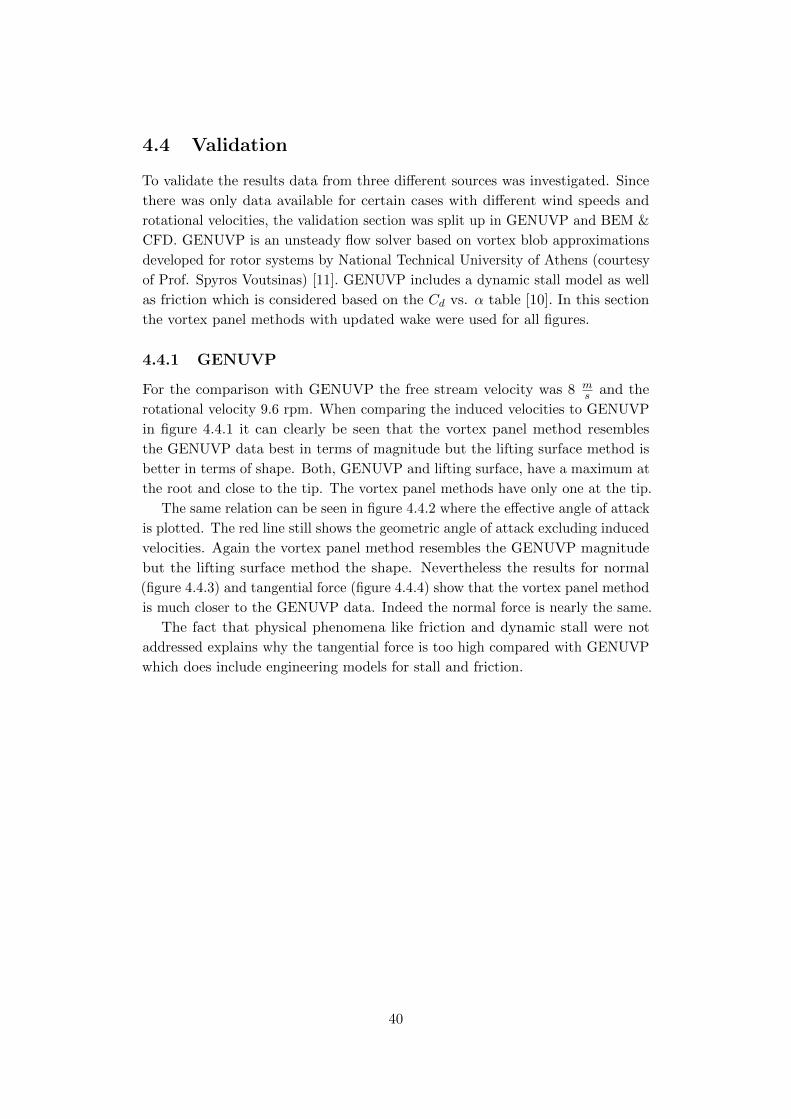
For the comparison with GENUVP the free stream velocity was 8 ms and the
rotational velocity 9.6 rpm. When comparing the induced velocities to GENUVP
in figure 4.4.1 it can clearly be seen that the vortex panel method resembles
the GENUVP data best in terms of magnitude but the lifting surface method is
better in terms of shape. Both, GENUVP and lifting surface, have a maximum at
the root and close to the tip. The vortex panel methods have only one at the tip.
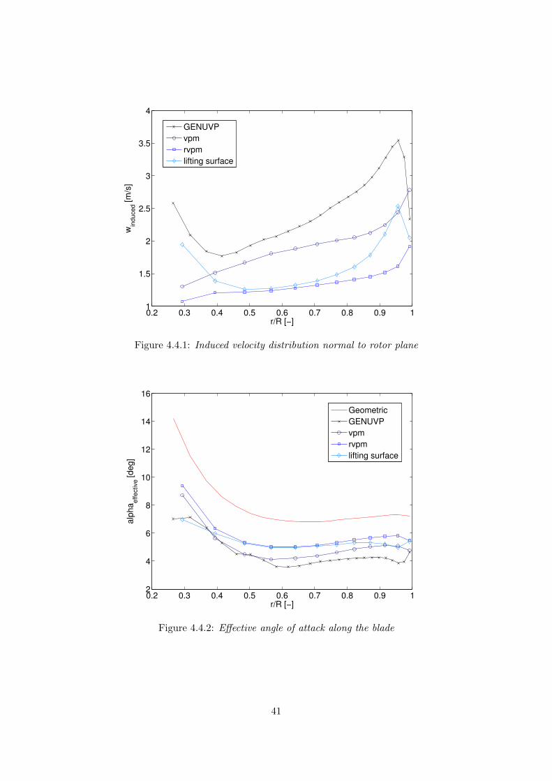
The same relation can be seen in figure 4.4.2 where the effective angle of attack
is plotted. The red line still shows the geometric angle of attack excluding induced
velocities. Again the vortex panel method resembles the GENUVP magnitude
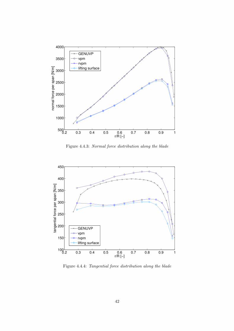
but the lifting surface method the shape. Nevertheless the results for normal
(figure 4.4.3) and tangential force (figure 4.4.4) show that the vortex panel method
is much closer to the GENUVP data. Indeed the normal force is nearly the same.
The fact that physical phenomena like friction and dynamic stall were not
addressed explains why the tangential force is too high compared with GENUVP
which does include engineering models for stall and friction.
40
0.2 0.3 0.4 0.5 0.6 0.7 0.8 0.9 11
1.5
2
2.5
3
3.5
4
r/R [−]
win
duced [m
/s]
GENUVP
vpm
rvpm
lifting surface
Figure 4.4.1: Induced velocity distribution normal to rotor plane
0.2 0.3 0.4 0.5 0.6 0.7 0.8 0.9 12
4
6
8
10
12
14
16
r/R [−]
alp
ha
effective [deg]
Geometric
GENUVP
vpm
rvpm
lifting surface
Figure 4.4.2: Effective angle of attack along the blade
41
0.2 0.3 0.4 0.5 0.6 0.7 0.8 0.9 1500
1000
1500
2000
2500
3000
3500
4000
r/R [−]
norm
al fo
rce p
er
span [N
/m]
GENUVP
vpm
rvpm
lifting surface
Figure 4.4.3: Normal force distribution along the blade
0.2 0.3 0.4 0.5 0.6 0.7 0.8 0.9 1100
150
200
250
300
350
400
450
r/R [−]
tangential fo
rce p
er
span [N
/m]
GENUVP
vpm
rvpm
lifting surface
Figure 4.4.4: Tangential force distribution along the blade
42

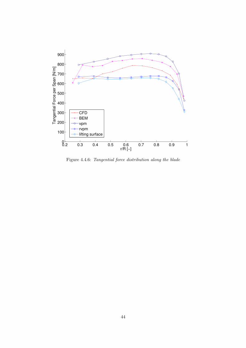
4.4.2 CFD & BEM
For every flow model it is important to compare the results with CFD if ex-
perimental data is not available since CFD is considered to be most accurate.
Furthermore the results are compared to BEM data, because BEM is very fast
and suitable for wind turbine analysis. Therefore it is a good reference for vortex
methods. Here the free stream velocity is 11.4 ms and the rotational velocity is
12.1 rpm.
Again the vortex panel method gives very good results for the normal force
distribution (figure 4.4.5), even better than BEM. But when it comes to tangential
forces (figure 4.4.6) the vortex panel method can not compete with BEM. Surpris-
ingly even the reduced vortex panel method is closer to the CFD data than VPM.
However, as mentioned in section 4.4.1 ”GENUVP”, all vortex panel methods
neglect the influence of dynamic stall and friction. Therefore the results should be
lower when including those. Then the results of the vortex panel method should
be closer to the CFD data.
0.2 0.3 0.4 0.5 0.6 0.7 0.8 0.9 11000
2000
3000
4000
5000
6000
7000
8000
r/R [−]
Norm
al F
orc
e p
er
Span [N
/m]
CFD
BEM
vpm
rvpm
lifting surface
Figure 4.4.5: Normal force distribution along the blade
43
0.2 0.3 0.4 0.5 0.6 0.7 0.8 0.9 10
100
200
300
400
500
600
700
800
900
r/R [−]
Tangential F
orc
e p
er
Span [N
/m]
CFD
BEM
vpm
rvpm
lifting surface
Figure 4.4.6: Tangential force distribution along the blade
44

5 Conclusion
In conclusion can be said, that the vortex panel method is very suitable for wind
turbine analysis. Although engineering models for stall and friction were not
included in the calculation the results of a basic vortex panel method are similar
to CFD and GENUVP data. In particular the normal force with respect to the
rotor plane is captured by the vortex panel method accurately.
Simpler vortex methods as the reduced vortex panel method and the lifting
surface method are much faster that the vortex panel method, but they should
not be used to model wind turbine blades. Since they neglect the curvature of
the camber line they are not able to produce accurate enough results.
Therefore choosing the right grid is very important for vortex panel methods.
Especially along the camber line there should not be any simplifications, which
means the grid should be very fine.
5.1 Future work
In order to prove the advantages of vortex panel methods compared to BEM it is
important to test it for unsteady conditions such as changing wind speeds and
non-uniform flows. Therefore the free vortex concept must be applied to such
flows.
Furthermore the root of the blade, the hub and the tower of the wind turbine
should be included in the model so that the influence of the whole wind turbine
is taken into account. However the vortex panel method itself can be improved
as well. Engineering models like dynamic stall models, dynamic inflow, friction
or wind turbulence can be included in the code.
45

A Appendices
A.1 Methods to simulate flow fields
A.1.1 BEM
Blade Element Momentum Theory combines two methods that analyze the
aerodynamics of wind turbines. The first method is to use a momentum balance
on a rotating stream tube in which a turbine is placed. The second one is to
examine the forces generated by the airfoil lift and drag coefficients at various
sections along the blade. These two methods then give a series of equations that
can be solved iteratively. [6] For more information see also [1].
A.1.2 CFD
Computational Fluid Dynamics (CFD) uses numerical methods and algorithms
to solve and analyze problems that concern fluid flows. That involves the solution
of the Navier-Stokes equation in fluid dynamics.
A.2 Airfoil geometries
0 0.2 0.4 0.6 0.8 1
−0.3
−0.2
−0.1
0
0.1
0.2
0.3
chord
thikness
Figure A.2.1: Airfoil geometry DU40 A17
46

0 0.2 0.4 0.6 0.8 1
−0.3
−0.2
−0.1
0
0.1
0.2
0.3
chord
thikness
Figure A.2.2: Airfoil geometry DU35 A17
0 0.2 0.4 0.6 0.8 1
−0.4
−0.3
−0.2
−0.1
0
0.1
0.2
0.3
chord
thikness
Figure A.2.3: Airfoil geometry DU30 A17
47
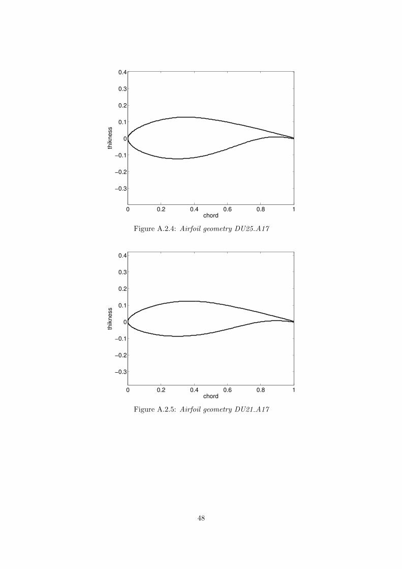
0 0.2 0.4 0.6 0.8 1
−0.3
−0.2
−0.1
0
0.1
0.2
0.3
0.4
chord
thikness
Figure A.2.4: Airfoil geometry DU25 A17
0 0.2 0.4 0.6 0.8 1
−0.3
−0.2
−0.1
0
0.1
0.2
0.3
0.4
chord
thikness
Figure A.2.5: Airfoil geometry DU21 A17
48

0 0.2 0.4 0.6 0.8 1
−0.3
−0.2
−0.1
0
0.1
0.2
0.3
0.4
chord
thikness
Figure A.2.6: Airfoil geometry NACA64 618
49
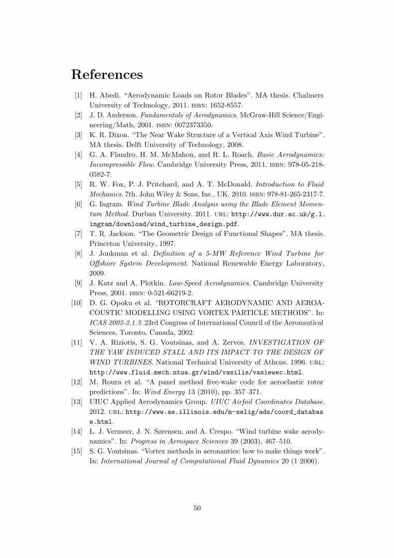
References
[1] H. Abedi. “Aerodynamic Loads on Rotor Blades”. MA thesis. Chalmers
University of Technology, 2011. isbn: 1652-8557.
[2] J. D. Anderson. Fundamentals of Aerodynamics. McGraw-Hill Science/Engi-
neering/Math, 2001. isbn: 0072373350.
[3] K. R. Dixon. “The Near Wake Structure of a Vertical Axis Wind Turbine”.
MA thesis. Delft University of Technology, 2008.
[4] G. A. Flandro, H. M. McMahon, and R. L. Roach. Basic Aerodynamics:
Incompressible Flow. Cambridge University Press, 2011. isbn: 978-05-218-
0582-7.
[5] R. W. Fox, P. J. Pritchard, and A. T. McDonald. Introduction to Fluid
Mechanics. 7th. John Wiley & Sons, Inc., UK, 2010. isbn: 978-81-265-2317-7.
[6] G. Ingram. Wind Turbine Blade Analysis using the Blade Element Momen-
tum Method. Durban University. 2011. url: http://www.dur.ac.uk/g.l.
ingram/download/wind_turbine_design.pdf.
[7] T. R. Jackson. “The Geometric Design of Functional Shapes”. MA thesis.
Princeton University, 1997.
[8] J. Jonkman et al. Definition of a 5-MW Reference Wind Turbine for
Offshore System Development. National Renewable Energy Laboratory,
2009.
[9] J. Katz and A. Plotkin. Low-Speed Aerodynamics. Cambridge University
Press, 2001. isbn: 0-521-66219-2.
[10] D. G. Opoku et al. “ROTORCRAFT AERODYNAMIC AND AEROA-
COUSTIC MODELLING USING VORTEX PARTICLE METHODS”. In:
ICAS 2002-2.1.3. 23rd Congress of International Council of the Aeronautical
Sciences, Toronto, Canada, 2002.
[11] V. A. Riziotis, S. G. Voutsinas, and A. Zervos. INVESTIGATION OF
THE YAW INDUCED STALL AND ITS IMPACT TO THE DESIGN OF
WIND TURBINES. National Technical University of Athens. 1996. url:
http://www.fluid.mech.ntua.gr/wind/vasilis/vasiewec.html.
[12] M. Roura et al. “A panel method free-wake code for aeroelastic rotor
predictions”. In: Wind Energy 13 (2010), pp. 357–371.
[13] UIUC Applied Aerodynamics Group. UIUC Airfoil Coordinates Database.
2012. url: http://www.ae.illinois.edu/m-selig/ads/coord_databas
e.html.
[14] L. J. Vermeer, J. N. Sørensen, and A. Crespo. “Wind turbine wake aerody-
namics”. In: Progress in Aerospace Sciences 39 (2003), 467–510.
[15] S. G. Voutsinas. “Vortex methods in aeronautics: how to make things work”.
In: International Journal of Computational Fluid Dynamics 20 (1 2006).
50