AERODYNAMIC PARAMETER ESTIMATION OF A MISSILE

A THESIS SUBMITTED TO

THE GRADUATE SCHOOL OF NATURAL AND APPLIED SCIENCES

OF

MIDDLE EAST TECHNICAL UNIVERSITY

BY

ARDA AKSU

IN PARTIAL FULFILLMENT OF THE REQUIREMENTS

FOR

THE DEGREE MASTER OF SCIENCE

IN

AEROSPACE ENGINEERING

SEPTEMBER 2013

Approval of the thesis:

AERODYNAMIC PARAMETER ESTIMATION OF A MISSILE

submitted by ARDA AKSU in partial fulfillment of the requirements for the degree of

Master of Science in Aerospace Engineering Department, Middle East Technical

University by,

Prof. Dr. Canan Özgen ______________

Dean, Graduate School of Natural and Applied Sciences

Prof. Dr. Ozan Tekinalp ______________

Head of Department, Aerospace Engineering

Asst. Prof. Dr. Ali Türker Kutay ______________

Supervisor, Aerospace Engineering Dept., METU

Examining Committee Members:

Prof. Dr. Kemal Leblebicioğlu ______________

Electrical and Electronics Engineering Dept., METU

Asst. Prof. Dr. Ali Türker Kutay ______________

Aerospace Engineering Dept., METU

Prof. Dr. Ozan Tekinalp ______________

Aerospace Engineering Dept., METU

Asst. Prof. Dr. İlkay Yavrucuk ______________

Aerospace Engineering Dept., METU

Dr. Gökmen Mahmutyazıcıoğlu ______________

Roketsan Missile Industries Inc.

Date: ______________

iv

I hereby declare that all information in this document has been obtained and presented

in accordance with academic rules and ethical conduct. I also declare that, as required

by these rules and conduct, I have fully cited and referenced all material results that

are not original to this work.

Name, Last Name : Arda Aksu

Signature :

v

ABSTRACT

AERODYNAMIC PARAMETER ESTIMATION OF A MISSILE

Aksu, Arda

M.Sc., Department of Aerospace Engineering

Supervisor Asst. Prof. Dr. Ali Türker Kutay

September 2013, 63 pages

Aerodynamic characteristics of missiles depend strongly on wind angles, that is, angle of

attack and sideslip angle. However it is impractical to measure these angles during missile

testing. Therefore, without direct information of the wind angles, it becomes a difficult

problem to be able to accurately estimate the missile aerodynamic parameters from flight

tests. This thesis addresses this problem and suggests an approach to estimate missile

aerodynamic parameters successfully without wind angles measurements. Instead of

reconstructing wind angles with post-process calculations prior to estimation, reconstruction

process is handled within the estimation. The algorithm developed is tested with simulated

missile data. Results are compared with true values used in simulation. It is demonstrated

that suggested approach can provide accurate and reliable estimations without wind angles

measurements. The approach is also applied to real flight test data of a missile with success.

Keywords: Missile, Open Loop Simulation, Parameter Estimation, Maximum Likelihood

vi

ÖZ

BİR FÜZENİN AERODİNAMİK PARAMETRE TAHMİNİ

Aksu, Arda

Yüksek Lisans, Havacılık ve Uzay Mühendisliği Bölümü

Tez Yöneticisi: Yrd. Doç. Dr. Ali Türker Kutay

Eylül 2013, 63 sayfa

Füzelerin aerodinamik karakteristikleri baskın olarak rüzgar açılarına bağlıdır. Fakat uçuşlu

testler sırasında bu açıların ölçümü pratik olmamaktadır. Bu yüzden bir füzenin aerodinamik

parametrelerinin uçuşlu testlerden düzgün bir şekilde tahmin edilebilmesi de zor bir problem

haline gelmektedir. Bu tez, bu problemi konu alarak bir füzenin aerodinamik

parametrelerinin rüzgar açıları ölçümü olmadan başarılı bir şekilde tahmin edilebilmesi için

bir yaklaşım önermektedir. Rüzgar açıları verilerinin tahmin çalışmasında kullanılmak üzere

yeniden yapılandırılması yerine, bu yapılandırma tahmin sırasında ele alınmaktadır.

Geliştirilen tahmin algoritması modellenen bir füzenin benzetim sonuçları üzerinde

denenmiştir. Tahminden elde edilen sonuçlar benzetimde kullanılan gerçek değerler ile

karşılaştırılarak, önerilen yaklaşımın rüzgar açılarının mevcut olmadığı durumda doğru ve

güvenilir sonuçlar verebileceği gösterilmiştir. Yaklaşım aynı zamanda gerçek bir atışlı test

verisine de başarıyla uygulanmıştır.

Anahtar Kelimeler: Füze, Açık Döngü Benzetim, Parametre Tahmini, Maksimum Olasılık

vii

To all who has ever taught me

viii

ACKNOWLEDGEMENTS

First of all, I would like to express my gratitude to my supervisor Asst. Prof. Dr. Ali Türker

Kutay for his patience and guidance throughout this study.

I would also like to thank to Gökmen Mahmutyazıcıoğlu, Tolga Avcıoğlu, Güneş Aydın,

Koray Erer, Alp Marangoz, Tayfun Çimen for their criticism and insight into the topic.

I would like to acknowledge my superiors and colleagues in Roketsan Missiles Industries for

their support to this study.

I am forever grateful to my wife Tuğçe Aksu, my parents Şaziye and Mehmet Aksu and my

sister Gözde Aksu. I always felt their love and confidence on me. Without their presence,

this thesis would not have been possible.

ix

TABLE OF CONTENTS

ABSTRACT ............................................................................................................................. v

ÖZ ........................................................................................................................................... vi

ACKNOWLEDGEMENTS .................................................................................................. viii

TABLE OF CONTENTS ........................................................................................................ ix

LIST OF FIGURES ................................................................................................................ xi

LIST OF TABLES ................................................................................................................. xii

NOMENCLATURE ............................................................................................................. xiii

CHAPTERS ............................................................................................................................. 1

1. INTRODUCTION ............................................................................................................... 1

1.1. Literature Review .......................................................................................................... 1

1.2. Problem Definition and Contribution of Thesis ............................................................ 2

1.3. Scope ............................................................................................................................. 3

2. MISSILE FLIGHT SIMULATION ..................................................................................... 5

2.1. Javelin ATGM .............................................................................................................. 5

2.2. Reference Frames and Modeling Assumptions............................................................. 6

2.3. Equations of Motion ..................................................................................................... 7

2.4. Aerodynamic Model ..................................................................................................... 8

3. EXPERIMENT DESIGN ................................................................................................... 11

3.1. Aerodynamic Model Verification ............................................................................... 11

3.2. Test Scenario ............................................................................................................... 14

3.3. Input Design ................................................................................................................ 15

4. ESTIMATION ALGORITHM .......................................................................................... 21

4.1. Optimization ............................................................................................................... 23

4.1.1. Noise Covariance Matrix ..................................................................................... 24

4.1.2. Parameter Update ................................................................................................. 24

4.1.3. Output Sensitivities .............................................................................................. 28

4.2. System Models ............................................................................................................ 28

4.2.1. Implicit Model ..................................................................................................... 29

4.2.2. Explicit Model ..................................................................................................... 31

5. ESTIMATION RESULTS ................................................................................................. 35

5.1. Sample Test Case ........................................................................................................ 35

5.2. Monte-Carlo Analysis ................................................................................................. 43

x

5.3. Real Flight Test ........................................................................................................... 45

6. CONCLUSIONS ................................................................................................................ 51

REFERENCES ....................................................................................................................... 53

APPENDICES ........................................................................................................................ 55

A. AIRCRAFT APPLICATION ............................................................................................ 55

xi

LIST OF FIGURES

FIGURES

Figure 2.1 - Launch picture of Javelin ATGM ........................................................................ 5

Figure 2.2 - Reference frames .................................................................................................. 6

Figure 2.3 - Dimensions (in mm) of Javelin ATGM ............................................................... 9

Figure 3.1 - Pitch plane static coefficients ............................................................................. 13

Figure 3.2 - Velocity plots for free flights with different initial pitch angles ........................ 15

Figure 3.3 - Aerodynamic force and moment derivatives ...................................................... 16

Figure 3.4 - Control surface deflections in studied test case .................................................. 17

Figure 3.5 - Wind angles in studied test case ......................................................................... 18

Figure 3.6 - Comparison of aerodynamic models .................................................................. 19

Figure 4.1 - Maximum Likelihood estimation loop ............................................................... 27

Figure 4.2 - Flow chart of implicit system model .................................................................. 31

Figure 4.3 - Flowchart of explicit system model ................................................................... 34

Figure 5.1 - Implicit model response with initial unknowns ................................................. 37

Figure 5.2 - Explicit model response with initial unknowns ................................................. 37

Figure 5.3 - Implicit model response with final estimates ..................................................... 38

Figure 5.4 - Explicit model response with final estimates ..................................................... 38

Figure 5.5 - Translational acceleration errors of implicit and explicit models ...................... 39

Figure 5.6 - Wind angle errors of implicit and explicit models ............................................. 40

Figure 5.7 - Update of aerodynamic parameters in sample case ............................................ 41

Figure 5.8 - Monte-Carlo results of implicit and explicit models .......................................... 45

Figure 5.9 - Convergence plots of flight test estimation ........................................................ 47

Figure 5.10 - Comparisons of flight test measurements and model outputs .......................... 48

Figure 5.11 - Errors from measurements ............................................................................... 49

xii

LIST OF TABLES

TABLES

Table 2.1 - Javelin ATGM Specifications After Burn-out ....................................................... 6

Table 2.2 - Input vectors of aerodynamic database .................................................................. 9

Table 3.1 - Aerodynamic moment derivatives at 0.4M .......................................................... 12

Table 3.2 - Parameters of linear model obtained with least square fit ................................... 18

Table 5.1 - True values and initial estimates used in sample test case ................................... 35

Table 5.2 - Estimated values with implicit and explicit models ............................................. 36

Table 5.3 - Correlations higher than 0.9 in implicit model results ......................................... 39

Table 5.4 - Estimated values with explicit model .................................................................. 42

Table 5.5 - Correlations higher than 0.9 in pitch plane explicit model results ....................... 43

Table 5.6 - True values and initial errors of unknown parameters ......................................... 44

xiii

NOMENCLATURE

, , p q r body axis angular rates (roll, pitch, yaw)

, , x y za a a body axis translational accelerations

, , u v w body axis velocities

, , x y z earth axis positions

, , Euler angles (roll, pitch, yaw)

, wind angles (angle of attack, sideslip angle)

, , e r a control surface deflections (elevator, rudder, aileron)

V total velocity relative to air

, , X Y ZC C C body axis non-dimensional aerodynamic force coefficients

, , l m nC C C body axis non-dimensional aerodynamic moment coefficients

, , , xx yy zz xzJ J J J mass moments of inertia

b reference span

l reference length

S reference area

air density

q dynamic pressure

sounda sound speed

m mass

g gravitational acceleration

xiv

1

CHAPTER 1

CHAPTERS

1. INTRODUCTION

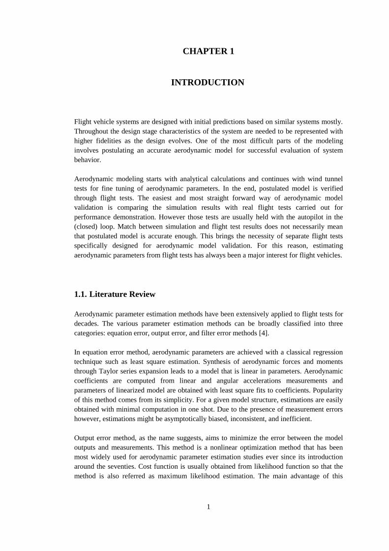
Flight vehicle systems are designed with initial predictions based on similar systems mostly.

Throughout the design stage characteristics of the system are needed to be represented with

higher fidelities as the design evolves. One of the most difficult parts of the modeling

involves postulating an accurate aerodynamic model for successful evaluation of system

behavior.

Aerodynamic modeling starts with analytical calculations and continues with wind tunnel

tests for fine tuning of aerodynamic parameters. In the end, postulated model is verified

through flight tests. The easiest and most straight forward way of aerodynamic model

validation is comparing the simulation results with real flight tests carried out for

performance demonstration. However those tests are usually held with the autopilot in the

(closed) loop. Match between simulation and flight test results does not necessarily mean

that postulated model is accurate enough. This brings the necessity of separate flight tests

specifically designed for aerodynamic model validation. For this reason, estimating

aerodynamic parameters from flight tests has always been a major interest for flight vehicles.

1.1. Literature Review

Aerodynamic parameter estimation methods have been extensively applied to flight tests for

decades. The various parameter estimation methods can be broadly classified into three

categories: equation error, output error, and filter error methods [4].

In equation error method, aerodynamic parameters are achieved with a classical regression

technique such as least square estimation. Synthesis of aerodynamic forces and moments

through Taylor series expansion leads to a model that is linear in parameters. Aerodynamic

coefficients are computed from linear and angular accelerations measurements and

parameters of linearized model are obtained with least square fits to coefficients. Popularity

of this method comes from its simplicity. For a given model structure, estimations are easily

obtained with minimal computation in one shot. Due to the presence of measurement errors

however, estimations might be asymptotically biased, inconsistent, and inefficient.

Output error method, as the name suggests, aims to minimize the error between the model

outputs and measurements. This method is a nonlinear optimization method that has been

most widely used for aerodynamic parameter estimation studies ever since its introduction

around the seventies. Cost function is usually obtained from likelihood function so that the

method is also referred as maximum likelihood estimation. The main advantage of this

2

method over equation error method is that aerodynamic parameters can be implemented in

state equations while minimizing the error. This in turn results with more accurate models.

In output error method, process noise in states is neglected and only measurement noise is

accounted. The filter error method on the other hand accounts for both process and

measurement noises and is the most general stochastic approach to aerodynamic parameter

estimation. Process noise is included in state equations so that minor errors in system model

can be eliminated with a state filter. In the presence of atmospheric turbulence this method is

known to yield accurate results [10].

In addition to methods above, frequency domain approaches might be preferable over time

domain approaches for rotorcraft identification [4]. Since no integration is involved in the

frequency domain, method becomes suitable for unstable systems for which numerical

integration in time domain can lead to problems. Moreover, without affecting the estimation

results, the zero frequency can be neglected in evaluation, which can be advantageous in

eliminating the need to bias parameters.

Other approaches appear in the literature are filtering approach which provides real time

estimations and neural network based methods for highly nonlinear aerodynamic models.

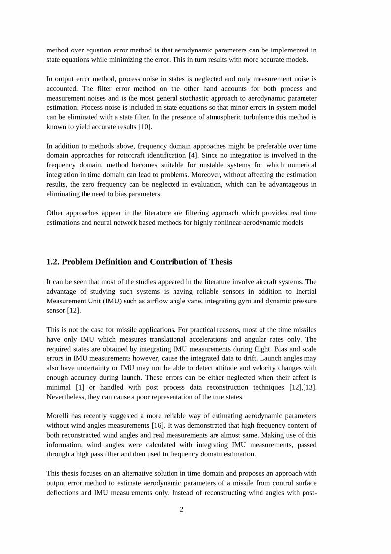
1.2. Problem Definition and Contribution of Thesis

It can be seen that most of the studies appeared in the literature involve aircraft systems. The

advantage of studying such systems is having reliable sensors in addition to Inertial

Measurement Unit (IMU) such as airflow angle vane, integrating gyro and dynamic pressure

sensor [12].

This is not the case for missile applications. For practical reasons, most of the time missiles

have only IMU which measures translational accelerations and angular rates only. The

required states are obtained by integrating IMU measurements during flight. Bias and scale

errors in IMU measurements however, cause the integrated data to drift. Launch angles may

also have uncertainty or IMU may not be able to detect attitude and velocity changes with

enough accuracy during launch. These errors can be either neglected when their affect is

minimal [1] or handled with post process data reconstruction techniques [12],[13].

Nevertheless, they can cause a poor representation of the true states.

Morelli has recently suggested a more reliable way of estimating aerodynamic parameters

without wind angles measurements [16]. It was demonstrated that high frequency content of

both reconstructed wind angles and real measurements are almost same. Making use of this

information, wind angles were calculated with integrating IMU measurements, passed

through a high pass filter and then used in frequency domain estimation.

This thesis focuses on an alternative solution in time domain and proposes an approach with

output error method to estimate aerodynamic parameters of a missile from control surface

deflections and IMU measurements only. Instead of reconstructing wind angles with post-

3

process calculations prior to estimation, reconstruction process is proposed to be handled

within the estimation. Output error method is utilized for this purpose. Efficiency of the

algorithm developed is demonstrated with both simulation and real flight test data.

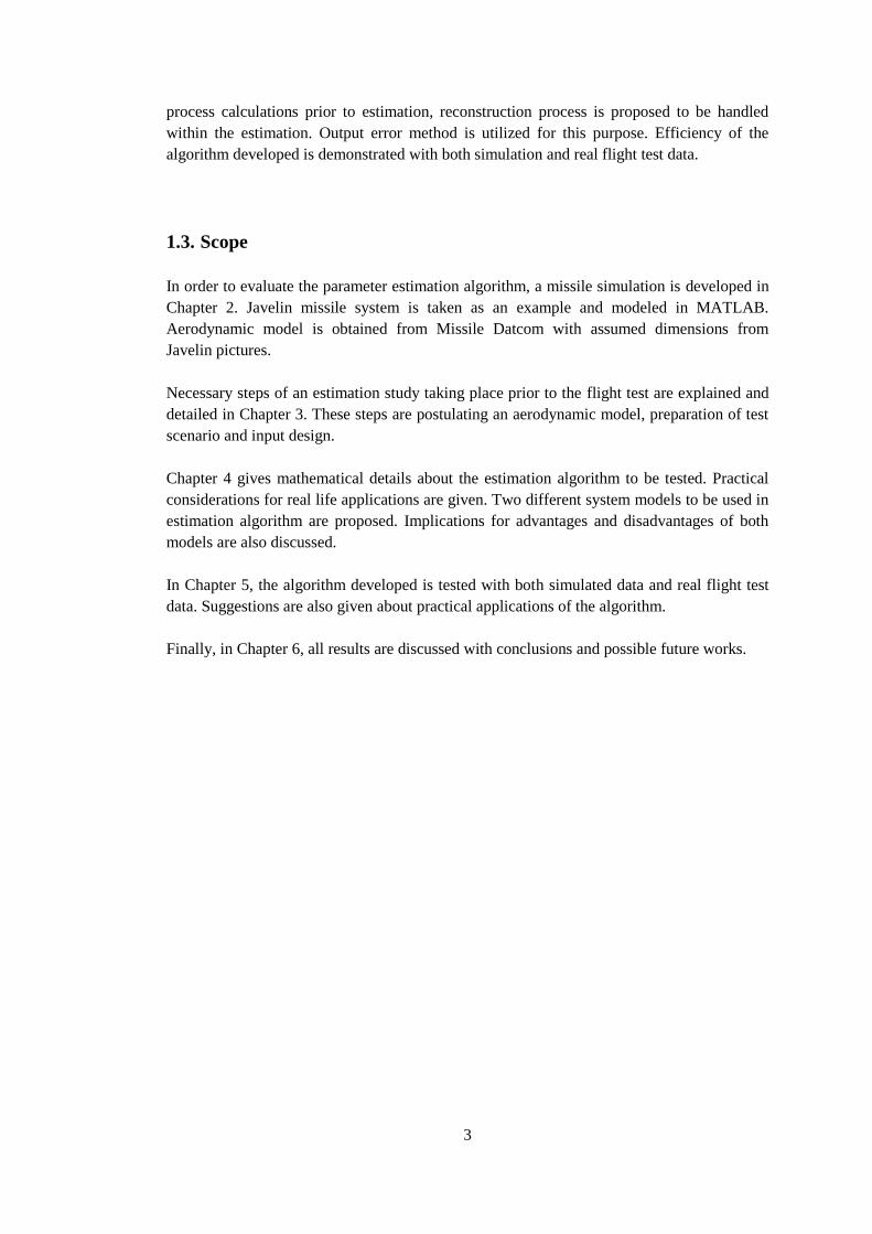
1.3. Scope

In order to evaluate the parameter estimation algorithm, a missile simulation is developed in

Chapter 2. Javelin missile system is taken as an example and modeled in MATLAB.

Aerodynamic model is obtained from Missile Datcom with assumed dimensions from

Javelin pictures.

Necessary steps of an estimation study taking place prior to the flight test are explained and

detailed in Chapter 3. These steps are postulating an aerodynamic model, preparation of test

scenario and input design.

Chapter 4 gives mathematical details about the estimation algorithm to be tested. Practical

considerations for real life applications are given. Two different system models to be used in

estimation algorithm are proposed. Implications for advantages and disadvantages of both

models are also discussed.

In Chapter 5, the algorithm developed is tested with both simulated data and real flight test

data. Suggestions are also given about practical applications of the algorithm.

Finally, in Chapter 6, all results are discussed with conclusions and possible future works.

4

5

CHAPTER 2

2. MISSILE FLIGHT SIMULATION

2.1. Javelin ATGM

Javelin Anti-Tank Guided Missile (ATGM) [6],[14] is a man-portable, fire-and-forget

system designed specifically to hit and destroy armored tanks and fighting vehicles. The

project has been managed by Texas Instrument (later changed as Raytheon) and Lockheed

Martin. Production phase has started in 1996 and missile has been used in field since then.

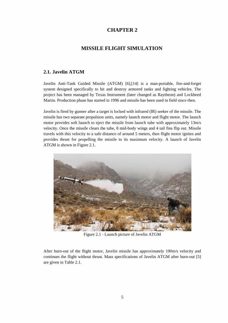
Javelin is fired by gunner after a target is locked with infrared (IR) seeker of the missile. The

missile has two separate propulsion units, namely launch motor and flight motor. The launch

motor provides soft launch to eject the missile from launch tube with approximately 13m/s

velocity. Once the missile clears the tube, 8 mid-body wings and 4 tail fins flip out. Missile

travels with this velocity to a safe distance of around 5 meters, then flight motor ignites and

provides thrust for propelling the missile to its maximum velocity. A launch of Javelin

ATGM is shown in Figure 2.1.

Figure 2.1 - Launch picture of Javelin ATGM

After burn-out of the flight motor, Javelin missile has approximately 190m/s velocity and

continues the flight without thrust. Mass specifications of Javelin ATGM after burn-out [5]

are given in Table 2.1.

6

Table 2.1 - Javelin ATGM Specifications After Burn-out

Mass 10.15 kg

Diameter 0.127 m

Length 1.081 m

CG (from nose) 0.446 m

JXX 0.023 kg m/s2

JYY , JZZ 0.914 kg m/s2

2.2. Reference Frames and Modeling Assumptions

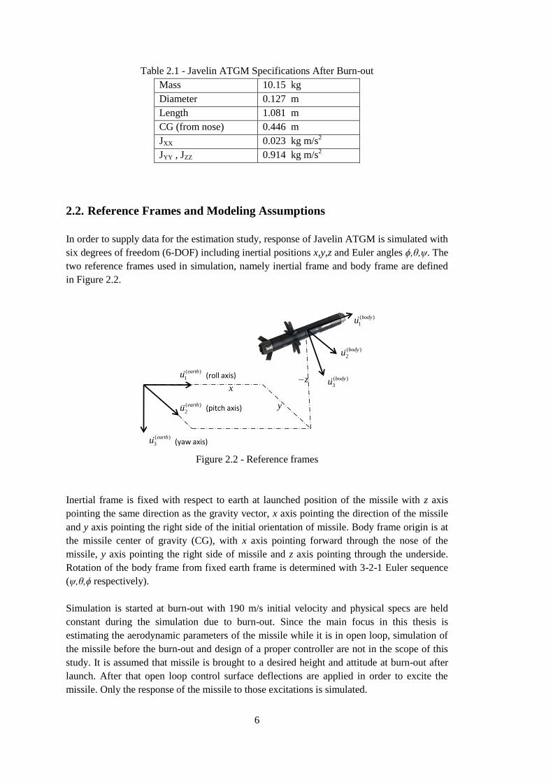
In order to supply data for the estimation study, response of Javelin ATGM is simulated with

six degrees of freedom (6-DOF) including inertial positions x,y,z and Euler angles ϕ,θ,ψ. The

two reference frames used in simulation, namely inertial frame and body frame are defined

in Figure 2.2.

Figure 2.2 - Reference frames

Inertial frame is fixed with respect to earth at launched position of the missile with z axis

pointing the same direction as the gravity vector, x axis pointing the direction of the missile

and y axis pointing the right side of the initial orientation of missile. Body frame origin is at

the missile center of gravity (CG), with x axis pointing forward through the nose of the

missile, y axis pointing the right side of missile and z axis pointing through the underside.

Rotation of the body frame from fixed earth frame is determined with 3-2-1 Euler sequence

(ψ,θ,ϕ respectively).

Simulation is started at burn-out with 190 m/s initial velocity and physical specs are held

constant during the simulation due to burn-out. Since the main focus in this thesis is

estimating the aerodynamic parameters of the missile while it is in open loop, simulation of

the missile before the burn-out and design of a proper controller are not in the scope of this

study. It is assumed that missile is brought to a desired height and attitude at burn-out after

launch. After that open loop control surface deflections are applied in order to excite the

missile. Only the response of the missile to those excitations is simulated.

( )

1

earthu

( )

2

earthu

( )

3

earthu

( )

1

bodyu

( )

2

bodyu

( )

3

bodyux

y

z(roll axis)

(pitch axis)

(yaw axis)

7

Further discussions of the assumptions made are given in the following sections.

2.3. Equations of Motion

The collected equations of motion of the missile to be used in the simulation are summarized

below [12]:

s 0

c s 0

c c 0

u r q uF

v g r p vm

w q p w

(2.1)

1

0 0 0 0 0

0 0 0 0 0

0 0 0 0 0

xx xx

yy yy

zz zz

p J r q J p

q J M r p J q

r J q p J r

(2.2)

1 s s / c s c / c

0 c s

0 s / c c / c

p

q

r

(2.3)

c c s c c s s s s c s c

s c c c s s s c s s s c

s c s c c

x u

y v

z w

(2.4)

where and are the resultant aerodynamic force and moment vectors acting on the

missile center of gravity expressed in the body coordinate frame. Note that sine() and

cosine() functions are denoted with s and c for simplicity. Aerodynamic forces and moments

are expressed in terms of non-dimensional aerodynamic coefficients as follows:

2

2

X

Y

Z

CV

F C S

C

(2.5)

2

2

l

m

n

CV

M C Sl

C

(2.6)

8

Gravitational acceleration, g and air density, ρ in the above equations are assumed not to

vary and used as constant in simulation. Considering the duration of the simulation and total

change in the altitude, this is a reasonable assumption.

State equations given above are numerically integrated in MATLAB using 2nd

order Runge-

Kutta integration with 1ms time step.

States and inputs of the missile model are defined as:

[ ]Tx u v w p q r x y z (2.7)

[ ]T

e r au (2.8)

The applied integration formula then can be shown as:

,

1 ,2

f x k u k dtx k x k f x k u k dt

(2.9)

where f is represented for the state function and u is represented for average value of the

current (k) and future (k+1) points.

2.4. Aerodynamic Model

Non-dimensional aerodynamic force and moment coefficients in equations (2.5) and (2.6)

are calculated using MISSILE DATCOM [2]. Geometric information of Javelin ATGM

obtained through a reference picture is given in Figure 2.3. Since the missile is symmetric in

XZ and XY planes, same coefficients are used for both planes.

As mentioned before, only the perturbed response of the missile in open loop is simulated in

a relatively small time interval. This is the key point for most of the assumptions made

especially in the aerodynamic model. Since the missile flies in a close vicinity of the ballistic

trajectory when small perturbations are given to the control surfaces, a small space around

reference condition is needed for the aerodynamic database. Vector of input breakpoints used

to determine the space of aerodynamic database are given in Table 2.2.

9

Figure 2.3 - Dimensions (in mm) of Javelin ATGM

Table 2.2 - Input vectors of aerodynamic database

Parameter Inputs

Mach [0.3 0.4 0.5 0.6]

, ,e ,

r ,a [-5 -4 -3 -2 -1 0 1 2 3 4 5] deg

Aerodynamic model using the parameters given in Table 2.2 are obtained from MISSILE

DATCOM in the following form:

( , , , , , )static

X X e r aC C M (2.10)

( , , ) ( )2r

static dynamic

Y Y r Y

rlC C M C M

V (2.11)

( , , ) ( )2q

static dynamic

Z Z e Z

qlC C M C M

V (2.12)

( , , , ) ( )2p

static dynamic

l l a l

plC C M C M

V (2.13)

( , , ) ( )2q

static dynamic

m m e m

qlC C M C M

V (2.14)

( , , ) ( )2r

static dynamic

n n r n

rlC C M C M

V (2.15)

Using the states and control surface deflection inputs in the simulation, each coefficient is

calculated with linear interpolation from the aerodynamic database at every time step. Total

velocity and wind angles are calculated from the states for no-wind condition as follows:

10

2 2 2V u v w (2.16)

1tan ( / )w u (2.17)

1tan ( / )v u (2.18)

Note that the flank angle representation is used for sideslip angle. This is a fair assumption

due to low attack angles.

One last assumption in the simulation is taking the speed of sound to be constant. Mach

number is then calculated as follows:

sound

VM

a (2.19)

11

CHAPTER 3

3. EXPERIMENT DESIGN

An aerodynamic parameter estimation study starts before the flight test. First an aerodynamic

model whose parameters are to be verified is determined. Then an appropriate test scenario is

prepared in which missile is held as long as possible in the region where the determined

model remains valid. Finally inputs whether in open loop or in close loop are designed so

that missile supplies rich content of information in its response. These are all parts of the

aerodynamic parameter estimation work that take place prior to flight. Before developing an

estimation algorithm, these steps are explained in detail below.

3.1. Aerodynamic Model Verification

In this study, identification of the aerodynamic model is restricted to Y and Z axes force and

moment coefficients. In other words only CZ and Cm coefficients are identified. Note that,

since missile is modeled as symmetric in pitch and yaw planes, CY and Cn are identical to CZ

and Cm in absolute values. There is only sign difference due to convention with:

static static

Z YC C (3.1)

q r

dynamic dynamic

Z YC C (3.2)

static static

m nC C (3.3)

q r

dynamic dynamic

m nC C (3.4)

Aerodynamic model is generally identified through parameters of linear expansion of the

model at a reference Mach number:

rrY Y Y r YC C C C r

(3.5)

qeZ Z Z e ZC C C C q

(3.6)

qem m m e mC C C C q

(3.7)

rrn n nn rC C C C r (3.8)

12

Since the aerodynamic models in pitch and yaw planes are same, common aerodynamic

derivatives are used also in linearized equations:

qeY Z Z r ZC C C C r

(3.9)

qeZ Z Z e ZC C C C q

(3.10)

qem m m e mC C C C q

(3.11)

qem mn r mC C C C r (3.12)

The goal of a parameter estimation study is to find the unknown parameters of a known

mathematical model. Here, the nonlinear aerodynamics of the missile is approximated by a

linear model and the parameters of this model will be estimated. The purpose of this section

is to find the linear model that best fits the actual nonlinear database. The linear model fitted

to the database will be used to evaluate the performance of the estimation methods in the

following sections.

Aerodynamic derivatives in linearized models are first evaluated from nonlinear database

directly as reference values. A reference Mach number is selected with considering the mean

velocity of the missile during the perturbations and nonlinear model is linearized around a

reference point. Most general way of doing this is taking central difference around zero

points for near ballistic flights. While the linear model obtained from central difference

method can approximate the aerodynamic data well within a small neighborhood around the

reference point, approximation becomes less and less accurate as the operation point moves

away from the reference point. To overcome this inaccuracy, linear model can be determined

with a least square fit of database values within a region that will be explored during the

excitations, rather than at a single point at the reference flight condition. Parameters of a

linear model obtained with two approaches for 0.5 Mach number are given in Table 3.1. It

can be seen that relative error between two approaches are nearly %5 for control derivatives.

Table 3.1 - Aerodynamic moment derivatives at 0.4M

Central difference approach Least square approach

Czα (stability derivative) -18.489 -19.183

Czδ (control derivative) -2.573 -2.666

Cmα (stability derivative) -30.894 -31.781

Cmδ (control derivative) -12.118 -12.557

Note that linear model obtained with central difference approach is exact for [-1,+1] degrees

angle of attack and [-1,+1] degrees elevator deflection intervals. On the other hand least

square approach fits the nonlinear model with a better coverage. Linear models are plotted

on aerodynamic database values in Figure 3.1. It can be seen that linear model obtained with

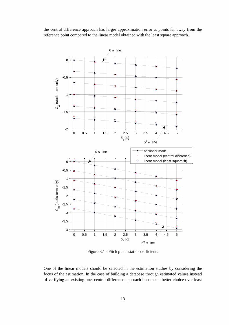
13

the central difference approach has larger approximation error at points far away from the

reference point compared to the linear model obtained with the least square approach.

Figure 3.1 - Pitch plane static coefficients

One of the linear models should be selected in the estimation studies by considering the

focus of the estimation. In the case of building a database through estimated values instead

of verifying an existing one, central difference approach becomes a better choice over least

0 0.5 1 1.5 2 2.5 3 3.5 4 4.5 5-2

-1.5

-1

-0.5

0

e [d]

CZ (

sta

tic t

erm

only

)

0 0.5 1 1.5 2 2.5 3 3.5 4 4.5 5

-4

-3.5

-3

-2.5

-2

-1.5

-1

-0.5

0

e [d]

Cm

(sta

tic t

erm

only

)

nonlinear model

linear model (central difference)

linear model (least square fit)

0 line

0 line

5o line

5o line

14

square approach. Parameters obtained through multiple flight test cases are put all together

and a final curve fit can be used for determination for a database model.

On the other hand, least square approach is better for studies that involve verification of an

existing model. Using the control surface deflections and angle of attack obtained -directly

or indirectly- from flight test as regressors, a least square fit is applied to nonlinear model for

determining the reference linear model. So that values obtained from estimation can be

compared with this reference model.

Either way, missile response must stay on the linear side of the real aerodynamic model as

much as possible during the perturbations applied for exciting the missile. So that time

invariant aerodynamic model used in estimation algorithm holds true in practice as well.

That being said, least square approach is preferred in this study for the verification of the

aerodynamic model used in simulation with estimation results.

Note that the static term in aerodynamic model created with Missile Datcom is linearized

with respect to wind angles, control surface deflections and Mach number while dynamic

term is linearized with respect to Mach number only.

3.2. Test Scenario

As explained before, estimation is applied to open loop response of the missile which flies

close to the ballistic trajectory, in other words around zero angle of attack and sideslip angle

after burn-out. Initial condition of this phase needs to be carefully determined with focusing

to create an interval with minimum velocity change during the perturbations. This ensures

that aerodynamic model can be estimated with a linearized expansion around a reference

Mach condition.

Altitude of the missile from ground level at burn-out is taken as 100m [5]. Simulation is

started from burn-out of the missile at that altitude with 190m/s velocity. Initial attitude of

missile -more specifically pitch angle- is needed to be determined next. Using a negative

pitch angle around -20 degrees provides the desired interval with minimum velocity change.

Unfortunately that does not appear to be a realistic scenario since the missile might hit the

ground too soon in such a trajectory. Instead, a relatively high pitch angle should be selected

so that missile can climb more and longer intervals to be used in estimation might be

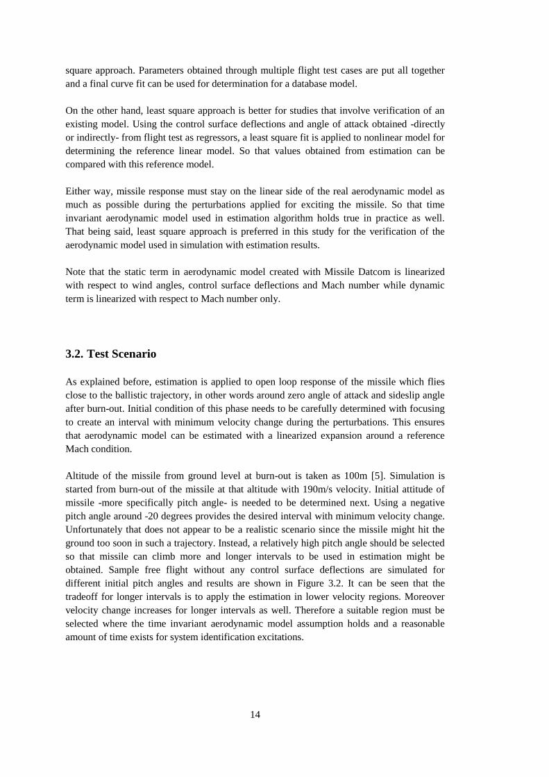
obtained. Sample free flight without any control surface deflections are simulated for

different initial pitch angles and results are shown in Figure 3.2. It can be seen that the

tradeoff for longer intervals is to apply the estimation in lower velocity regions. Moreover

velocity change increases for longer intervals as well. Therefore a suitable region must be

selected where the time invariant aerodynamic model assumption holds and a reasonable

amount of time exists for system identification excitations.

15

Figure 3.2 - Velocity plots for free flights with different initial pitch angles

Although it appears that in lower velocities there are longer intervals which might promise

better estimations naturally, it is critical to verify the aerodynamic model close to the

velocities which missile normally operates as far as possible. Therefore initial pitch angle is

selected as 30 degrees. Perturbations are applied between seconds 7 and 19 in 30o theta plot

in Figure 3.2. The difference between minimum and maximum velocity during the interval is

12.5 m/s which is represented with 0.037 Mach number in simulation. This should be an

acceptable change for the time invariant aerodynamic model assumption and is checked in

the next section.

3.3. Input Design

The objective of the input design is to excite the missile so that measurement data contains

sufficient information for a successful estimation. Since measurements are noisy, higher

excitations yields better signal to noise ratios. The practical difficulty that must be taken into

consideration while exciting the missile with higher amplitudes is to ensure that states stay in

the region required by the aerodynamic model used in estimation.

Note that dynamic terms in the aerodynamic model are already linear. Static terms are

linearized to be used in estimation. Those linear models are functions of wind angles and

control surface deflections. These parameters must stay on the linear region of real

aerodynamic model around zero points in order that linear aerodynamic model retains the

validity in that region and so it can give the same results with measurements. If the

parameters drift away from the linear region, no single linear model can closely approximate

the database anymore. This means there exists no parameter set that will cause the model

output to match the real missile behavior closely. In this case the estimation process will

produce inaccurate results or no results at all.

0 5 10 15 20 25100

120

140

160

180

200

time of flight [s] (starting from burn-out)

absolu

te v

elo

city [

m/s

]

0=0o

0=10o

0=20o

0=30o

0=40o

16

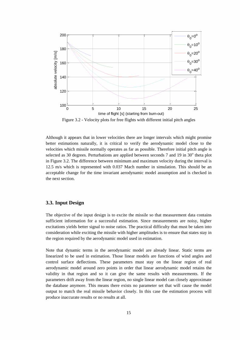
Local derivatives of pitch plane aerodynamic coefficients at 0.37 and 0.42 Mach numbers

(which are the minimum and maximum velocities within the test interval selected for

excitations) are given in Figure 3.3 with respect to angle of attack and elevator deflection. In

Y axis of plots, relative errors with respect to derivatives at zero angle of attack, zero

elevator deflection and mean velocity are also included.

Figure 3.3 - Aerodynamic force and moment derivatives

It can be seen that dominant relative error is in control derivatives due to angle of attack and

elevator deflection. After 4 degrees for both of those parameters, relative errors exceed the

%10 bands, above which linearity assumption might fail. Note that 0.04M velocity change

has a negligible effect on relative errors. In fact due to this reason, 12 sec interval discussed

above might be stretched little more with starting excitations earlier if it is necessary to

increase observability.

In order to provide high signal to noise ratio at measurements, missile should be excited near

the natural frequency of dominant dynamic mode while keeping the states in linear region at

-5 0 5

-20.1 %9

-19.5 %6

-18.9 %2

-18.4 %0

[d]

CZ stability derivative

-5 0 5

-2.8 %9

-2.7 %5

-2.6 %1

e [d]

CZ control derivative

-5 0 5

-33 %7

-32.2 %4

-31.4 %2

-30.7 %0

[d]

Cm

stability derivative

-5 0 5

-13.5 %12

-13 %7

-12.5 %3

-12.1 %0

e [d]

Cm

control derivative

e lines @0.37M

e lines @0.41M

lines @0.37M

lines @0.41M

17

the same time. If a parameter estimation study is intended to be applied without any prior

information about the aerodynamic model, missile should be excited over a broad frequency

range with nearly constant power for all frequencies. However this study focuses on

verification of an existing model so that all the information available prior to the estimation

can be used in input design stage.

Natural frequency of dominant dynamic mode must be determined first. The easiest and

practical way of doing this without analytical calculations is to apply frequency sweep input

in simulation and analyzing the frequency response of the missile. The frequency having the

highest amplitude in measurements is the dominant dynamic mode. Exciting the missile in

near frequencies provides better signal to noise ratios in measurements hence better

observability of aerodynamic parameters. Applying perturbed control surface deflections

with frequency which is same as the dynamic mode frequency and a suitable amplitude

chosen based on the linearity concerns gives a good starting point. Further fine tunings

should be made for better usage of linear model limits. Both frequency and amplitude of the

control surface deflections can be adjusted appropriately in order to design an optimal test

case. For example the dynamic mode of the Javelin ATGM at 0.4M is approximately 3.5Hz.

Applying control surface deflections with that frequency and 3 degrees amplitude to missile

causes wind angles to exceed 5 degrees which should not be accepted due to the limits of the

linear region. Either amplitude of the inputs should be lowered or frequency should be

moved further from dynamic mode to resolve this issue. First choice lowers the signal to

noise ratio obviously if control surface deflection measurements are noisy. Therefore

changing the input frequency is a better choice.

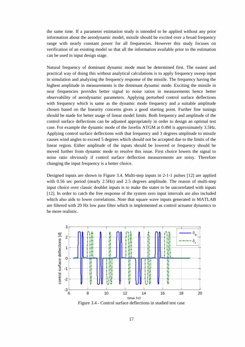
Designed inputs are shown in Figure 3.4. Multi-step inputs in 2-1-1 pulses [12] are applied

with 0.56 sec period (nearly 2.5Hz) and 2.5 degrees amplitude. The reason of multi-step

input choice over classic doublet inputs is to make the states to be uncorrelated with inputs

[12]. In order to catch the free response of the system zero input intervals are also included

which also aids to lower correlations. Note that square wave inputs generated in MATLAB

are filtered with 20 Hz low pass filter which is implemented as control actuator dynamics to

be more realistic.

Figure 3.4 - Control surface deflections in studied test case

6 8 10 12 14 16 18 20-3

-2

-1

0

1

2

3

time [s]

contr

ol surf

ace d

eflections [

d]

e

r

18

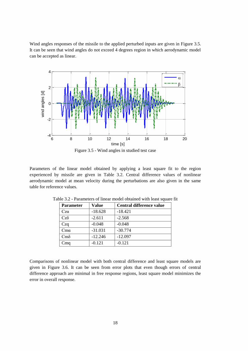
Wind angles responses of the missile to the applied perturbed inputs are given in Figure 3.5.

It can be seen that wind angles do not exceed 4 degrees region in which aerodynamic model

can be accepted as linear.

Figure 3.5 - Wind angles in studied test case

Parameters of the linear model obtained by applying a least square fit to the region

experienced by missile are given in Table 3.2. Central difference values of nonlinear

aerodynamic model at mean velocity during the perturbations are also given in the same

table for reference values.

Table 3.2 - Parameters of linear model obtained with least square fit

Parameter Value Central difference value

Czα -18.628 -18.421

Czδ -2.611 -2.568

Czq -0.048 -0.048

Cmα -31.031 -30.774

Cmδ -12.246 -12.097

Cmq -0.121 -0.121

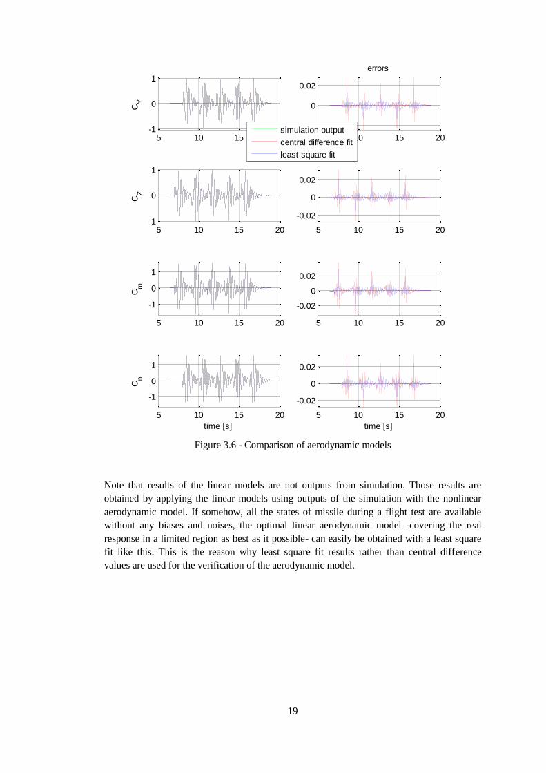
Comparisons of nonlinear model with both central difference and least square models are

given in Figure 3.6. It can be seen from error plots that even though errors of central

difference approach are minimal in free response regions, least square model minimizes the

error in overall response.

6 8 10 12 14 16 18 20-4

-2

0

2

4

time [s]

win

d a

ngle

s [

d]

19

Figure 3.6 - Comparison of aerodynamic models

Note that results of the linear models are not outputs from simulation. Those results are

obtained by applying the linear models using outputs of the simulation with the nonlinear

aerodynamic model. If somehow, all the states of missile during a flight test are available

without any biases and noises, the optimal linear aerodynamic model -covering the real

response in a limited region as best as it possible- can easily be obtained with a least square

fit like this. This is the reason why least square fit results rather than central difference

values are used for the verification of the aerodynamic model.

5 10 15 20-1

0

1

CY

5 10 15 20

-0.02

0

0.02

errors

5 10 15 20-1

0

1

CZ

5 10 15 20

-0.02

0

0.02

5 10 15 20

-1

0

1

Cm

5 10 15 20

-0.02

0

0.02

5 10 15 20

-1

0

1

Cn

time [s]

simulation output

central difference fit

least square fit

5 10 15 20

-0.02

0

0.02

time [s]

20

21

CHAPTER 4

4. ESTIMATION ALGORITHM

In general mathematical model of a dynamic system whose unknown parameters are to be

estimated is given by:

( )z y (4.1)

where z is the observation or measurement, is the (np x 1) unknown parameter vector, y is

the output function of the system model and v is the measurement noise. Then, based on the

Fisher estimation theory [11], likelihood function of independent random observations can

be defined as:

1

; | |N

i

i

L z p z p z

(4.2)

Above function is probability density of measured data as a function of system parameters,

. In other words, it is probability of measurements given system parameters. The

likelihood function gets the maximum value for true parameters. Therefore maximum

likelihood estimator for parameter vector is equal to that maximizes the likelihood

function for N measurements. This can be shown as follows:

1

ˆ max |N

i

i

p z

(4.3)

It is generally preferred to minimize the negative logarithm of likelihood function rather than

to maximize the likelihood function [8]. So that a suitable optimization technique can be

applied to the negative logarithm of the likelihood function which represents the cost

function:

11

ˆ min ln | min ln |N N

i i

ii

p z p z

(4.4)

Minimizing the negative logarithm instead of maximizing also comes with great numeric

stability. Since the maximum value of the likelihood function is between zero and one,

multiplying the likelihood functions of different measurements with each other repeatedly

gives eventually a small number which can’t be represented with enough precision in a

computer. To resolve this, scaling might be applied after each multiplication. However this

complicates the optimization technique to be used and brings computational burden as well.

Instead, the logarithm scales the result at each step naturally and increases the precision. Yet

22

the logarithm function is monotonic, so maximizing the logarithm functions can also be

achieved with minimizing the negative of it. Since minimization of a cost function is an

easier procedure than maximizing, negative logarithm of likelihood function is by far

advantageous over likelihood function alone.

Maximum likelihood estimation can be applied to any form of probability density function.

One of the most widely used density distribution for likelihood functions is Gaussian

distribution:

2

2

1exp

22

x mp x

(4.5)

where m is the expected value (mean) of x and is the covariance of x. Likelihood function

defined above was probability density of one observation parameter as a function of

unknown parameters. In case of observing parameters more than one, likelihood function

becomes the joint probability distribution of observations. Joint probability density function

of n Gaussian distributed random variables is given by:

11 1exp

22

T

np x x m R x m

R

(4.6)

R given above is the (n x n) covariance matrix of random variable vector. Assuming that

random variables are uncorrelated with each other, covariance matrix can be stated as

diagonal. Since mean values of the random variables represent the true outputs, joint

probability distribution of observations are stated as:

11 1exp

22

T

np z z y R z y

R

(4.7)

where z and y is the (n x 1) measurement and output vectors respectively. Note that (n x

n) covariance matrix is now represented for measurement noise z y . Likelihood function

of n independent Gaussian distributed random variables as N many observations each is then

given by:

1

11

1 1; | exp

22

N

N NT

i i i i in

ii

L z p z z y R z yR

(4.8)

By taking the negative logarithm of above function, cost function to be minimized for

estimating unknown parameters is obtained:

23

ln ;J L z (4.9)

1

1

lnln 2 1

2 2 2

NT

i i i i

i

N RnNJ z y R z y

(4.10)

4.1. Optimization

Minimization of the above function can be satisfied by setting the gradient to zero:

00

J

(4.11)

Using the first order Taylor series expansion as an approximation, the gradient of the cost

function is given by:

0 0

2

T

J J J

(4.12)

Setting the right hand side of above equation to zero and solving for gives:

00

12

T

J J

(4.13)

Above change in parameter vector makes local gradient zero at that point. With an initial

guess, iterative solution of above equation provides the parameter vector for the minimum

value of cost function. This approach is commonly known as Newton-Raphson optimization

in the literature.

The difficulty of applying this technique is that the covariance matrix given in the cost

function depends also on unknown parameters. This fact complicates the optimization

algorithm while taking the derivatives of cost. In fact mathematically speaking there is no

closed form solution of this problem. Instead of applying the minimization for the unknown

system parameters all at once, relaxation technique can be used. In this technique, covariance

matrix is assumed not to be affected by change in system parameters. It is used as constant in

cost function and after each parameter update it is updated independently for the new

parameters.

The procedure of the relaxation technique can be summarized as follows:

1. Set initial values for parameters.

24

2. Find system outputs for selected parameters and estimate the noise covariance

matrix from measurement errors.

3. Apply the optimization to minimize the cost function and update the unknown

parameter vector.

4. Iterate step 2 and 3 until convergence.

4.1.1. Noise Covariance Matrix

Estimation of the covariance matrix is obtained similarly. The gradient with respect to the

covariance matrix is set to zero and then solved for the covariance matrix. The first term in

the cost function has no effect on minimization. Dropping that term and rearranging the cost

function as follows as a function of covariance matrix makes easier to take the derivative.

1

1

ln 1

2 2

TN

T

i i i i

i

N RJ R R z y z y

(4.14)

Then partial derivative with respect to covariance matrix is obtained as:

1 1 1

1

1

2 2

NT

i i i i

i

J R NR R z y z y R

R

(4.15)

Setting the gradient to zero and solving for R gives the estimate of the noise covariance

matrix for the current values of parameters at that step:

1

1ˆN

T

i i i i

i

R z y z yN

(4.16)

After each parameter update, covariance matrix is calculated again. Estimated covariance

matrix is then used as constant while finding the parameter update.

4.1.2. Parameter Update

Since covariance matrix in the cost function is fixed at each step during the optimization,

cost to be minimized reduces to:

1

1

1

2

NT

i i i i

i

J z y R z y

(4.17)

The gradient of the cost function with respect to the parameter vector

25

1 1

1

1

2

T

NTi i i i

i i i i

i

z y z yJR z y z y R

(4.18)

Measurement vector is also independent from parameters. Simplifying above equation using

this gives:

1

1

TN

i

i i

i

yJR z y

(4.19)

The second order gradient of the cost function is given by:

22

1 1

1

T TN

i i i

i iT Ti

y y yJR z y R

(4.20)

The partial derivative of outputs with respect to the parameter vector is called response

gradient or output sensitivity. This is an (n x np) matrix with n is the number of output or

measurement variables and np is the number of unknown parameters or in other words length

of the parameter vector, . [i,j] element of the matrix is quantifies the change in ith

observation due to the change in jth parameter.

The first term in the summation above includes the second order gradient of the response.

This gradient is computationally expensive to obtain and generally suggested to be

neglected. Yet summation of products of the second order response gradients with residuals

converges to zero for the true parameters. For that reason neglecting this term is a good

approximation near the final solution. The algorithm obtained with this simplification is

known as Gauss-Newton method in the literature.

Combining the cost gradients in parameter change equation gives:

0 0

1

1 1

1 1

T TN N

i i i

i i

i i

y y yR R z y

(4.21)

In order the inversion of the second order cost gradient in the parameter change equation to

be successful, the necessary condition is having a full rank matrix inside. Since R is taken

diagonal as explained before, response gradients must be linearly independent to satisfy that

condition. In other words both rows and columns of the response gradients must be linearly

independent with each other.

This is only possible when system parameters to be estimated must have a unique impact on

outputs and those outputs are not correlated with each other. Otherwise second order cost

gradient becomes singular and inversion might simply fail.

26

Numerical errors might also be accounted for a nearly singular matrix. If inversion does not

fail, parameter change might result in with divergence in cost function. In order to prevent

this, inversion with singular value decomposition [15] might be a better way instead of direct

inversion.

Gauss-Newton method explained above is an unconstrained optimization starting from an

initial point based on a quadratic cost function assumption. In some circumstances such as

when the cost function is highly nonlinear or initial parameters are far away from the true

values, the step size of parameter vector might be too large during the iteration. Singular

value decomposition helps to detect the directions of large parameter changes [12]. Defining

an upper limit for the change helps the cost function to converge. However one limit might

not be applicable for all directions due to the difference of parameter scales. Instead, a

simpler approach based on heuristic considerations is commonly preferred. If the cost

function diverges at any step during the iteration, parameter update size is reduced by

halving each time until reduction in cost function is satisfied [8]. This is applied by

implementing a weight factor in parameter change equation as follows:

0 0

1

( 1) 1 1

1 1

2

T TN N

i i ik

i i

i i

y y yR R z y

(4.22)

where k is used as one at each iteration. If the cost increases, k is also increased by one until

the cost decreases during the iterations.

There are other methods also to prevent divergences such as bounding the parameters [7] and

switching to simplex method in cost increase [18] but halving approach is found to work fine

and is preferred in this study for its simplicity.

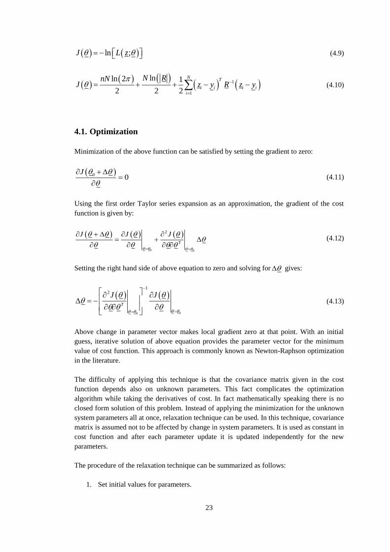
Parameter update process is repeated until a convergence criterion is satisfied. Assessment of

final convergence should be made for both relative changes in cost function and in

parameters at the same time. Estimation loop including parameter halving procedure is

presented in Figure 4.1.

27

Find parameter

update vector, Δθ

Find cost for

θ = θ0 + Δθ

Is cost decreased

relative to

previous cost?

Set

Δθ = Δθ / 2

no

Estimate noise

covariance matrix

Is convergence

criteria

satisfied?

yes

yes

Set

θ0 = θ

previous cost = cost

no

Terminate

Set initial θ0

Find cost for θ0

Figure 4.1 - Maximum Likelihood estimation loop

28

4.1.3. Output Sensitivities

Output sensitivities both in first and second order cost gradients can be found analytically by

taking partial derivatives of outputs with respect to unknown parameters. However in the

case of nonlinearity involved in the postulated output model analytical calculations might be

really complicated. Yet derivatives must be found again even if a minor modeling change in

the postulated model occurs. In order to deal with this difficulty, output sensitivities are

approximated with numerical differences.

Using central difference approximation for each parameter, jth column of the output

sensitivity matrix can be found as:

( ) ( )

2

j j

j j

j j

y y e y e

(4.23)

j given below is the perturbation step for the jth parameter.

je denotes a vector with one

in the jth element and zeroes elsewhere.

Perturbation size is generally chosen relative to the parameter to be perturbed. 0.1% of the

nominal value is found to be a reasonable choice. Also in case of the nominal value is too

small to be perturbed with this relative size, perturbation size must be limited with an

absolute lower bound.

4.2. System Models

As already stated in previous chapters, wind angles are one of the most important inputs for

the estimation process. Aerodynamic response depends strongly on angle of attack and

sideslip angle. Since these angles are not measured directly, they must be properly

represented in system model. To do so linear body velocities are reconstructed in system

model during the iterations and wind angles are computed from those parameters. The

assumption for that representation to be true is that there is no wind acting on the system.

Therefore flight test must be carried out in steady atmosphere with low level wind condition.

Since the focus is verifying the aerodynamic parameters through IMU measurements only,

outputs of the system model used in estimation must be restricted with translational

accelerations and angular rates.

Two different system models, namely implicit and explicit models are postulated to be used

in optimization of the maximum likelihood function. System models represented here are

continuous state equations and are numerically integrated to states with 2nd

order Runge-

Kutta integration method. Details of the models are given below in this section.

29

4.2.1. Implicit Model

Angle of attack and sideslip angle are determined implicitly in this model. Response of the

system to control surface deflections is obtained using dynamic system equations in pitch

and yaw planes whereas roll plane response is obtained by integrating measurements using

kinematic equations. Initial states are chosen as unknown with prior values and determined

through the optimization routine together with aerodynamic parameters. Bias errors in input

and output variables are also introduced as unknown parameters in the estimation.

For aerodynamic parameter estimation studies in the literature -conducted for aircraft

mostly- state models used in estimation algorithms are in similar forms [8],[12]. It can be

seen that almost every model uses the aerodynamic parameters to be estimated in state

equations. So that output of the estimation model becomes more reliable when matched with

real measurements. However, that would be a good approach only if there are several

measurements to verify the outputs with. In the case of limited number of measurements,

integration of states obtained purely from system model lacks robustness in estimation. Since

model outputs at any time involve historic data which might have been affected from any

modeling errors, observability problems may appear while trying to match them with

measurements. Since wind angles which are one of the most valuable information are

missing in this study, it is very likely that this model fails.

Input vector is given by:

[ ]T

e r xu p a (4.24)

States of the model are defined as:

[ ]Tx q r u v w (4.25)

Model outputs in order to match with measurements are:

[ ]T

y zy a a q r (4.26)

State equations of the postulated model can be shown as follows:

2 2 2 1

(1 / )

( ) ( tan ( / ) ) / 2 /qe

M M e M

x y

y

q J J pr

u v w Sl C w u C C q J

(4.27)

2 2 2 1

( / 1)

( ) ( tan ( / ) ) / 2 /qe

M

y

M r M

x

y

r J J pq

u v w Sl C v u C C r J

(4.28)

sin xu qw rv g a (4.29)

30

2 2 2 1

cos sin

( ) ( tan ( / ) ) / 2 /qe

Z Z r Z

v ru pw g

u v w S C v u C C r m

(4.30)

2 2 2 1

cos cos

( ) ( tan ( / ) ) / 2 /qe

Z Z e Z

w pv qu g

u v w S C w u C C q m

(4.31)

tan ( sin cos )p q r (4.32)

cos sinq r (4.33)

Note that same aerodynamic derivatives are used for both pitch and yaw planes as explained

in Section 3.1. Observation equations can be defined using inputs and states at each sample

point:

2 2 2 1( ) ( tan ( / ) ) / 2 /

qeZy Z r Za u v w S C v u C C r m

(4.34)

2 2 2 1( ) ( tan ( / ) ) / 2 /

qez Z Z e Za u v w S C w u C C q m

(4.35)

q q (4.36)

r r (4.37)

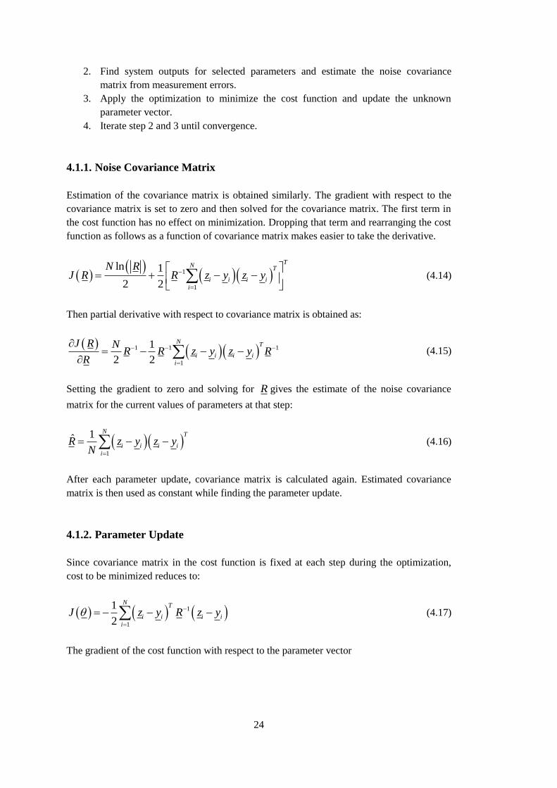
Previously stated disadvantage about error propagation can be clearly seen from equations

above. In order to represent the angle of attack and sideslip angle, integrated velocities are

used in observation equations. However neither the air flow angles nor those velocities are

available independently. This is the difficulty itself of estimating aerodynamic parameters

without any air flow angle information. The weighted parts of outputs come from the air

flow angle product term and for this reason air flow angle data must be carefully constructed.

However this model suffers from sensitivity since the integration in state equations highly

depends on the aerodynamic characteristics of model. Any modeling errors or relatively high

disturbances at any time in data might affect the whole optimization process.

Bias errors in measurements mentioned before are not included in both state equations and

observation equations. Since model is already nonlinear, those errors can be placed as

unknown parameters in inputs and outputs instead of using directly in equations to preserve

the simplicity of equations. Then, input and output vectors must be represented in the

following form:

[ ]x

T

e r p x au p b a b (4.38)

[ ]y z

T

y a z a q ry a b a b q b r b (4.39)

31

Note that control surface deflection measurements are assumed to be true without any bias

errors.

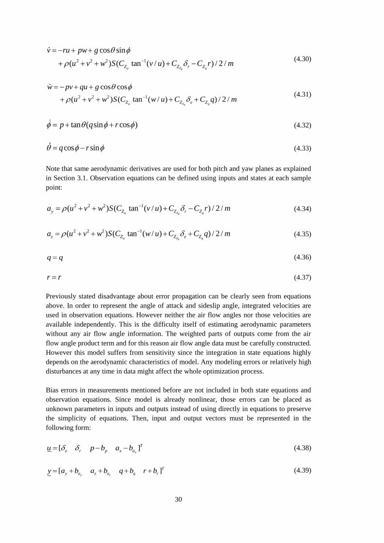
Flowchart of this model can be seen in Figure 4.2.

Figure 4.2 - Flow chart of implicit system model

4.2.2. Explicit Model

In order to deal with the air flow angles reconstruction nicely, an alternative approach in

model definition is studied. Rather than obtaining the angle of attack and sideslip angle by

using pure response of parameters to be estimated, response of the system from

measurements is used. In other words kinematic equations are preferred instead of dynamic

equations. So that angle of attack and sideslip angle are explicitly evaluated from input data

and take place in observation equations. Again initial states are also chosen as unknown.

Input and output biases for this model are more important and have more impact on

estimation results than before.

Inputs are control surface deflections, translational accelerations and angular rates:

[ ]x y z

T

e r p q r x a y a z au p b q b r b a b a b a b (4.40)

IMU measurements used for verifying the model outputs are also used as inputs in this

model. The reason for this approach is to carry some information with input data and

decouple the effects of control surface inputs and body motion in outputs.

States of the model are linear body velocities and Euler angles:

32

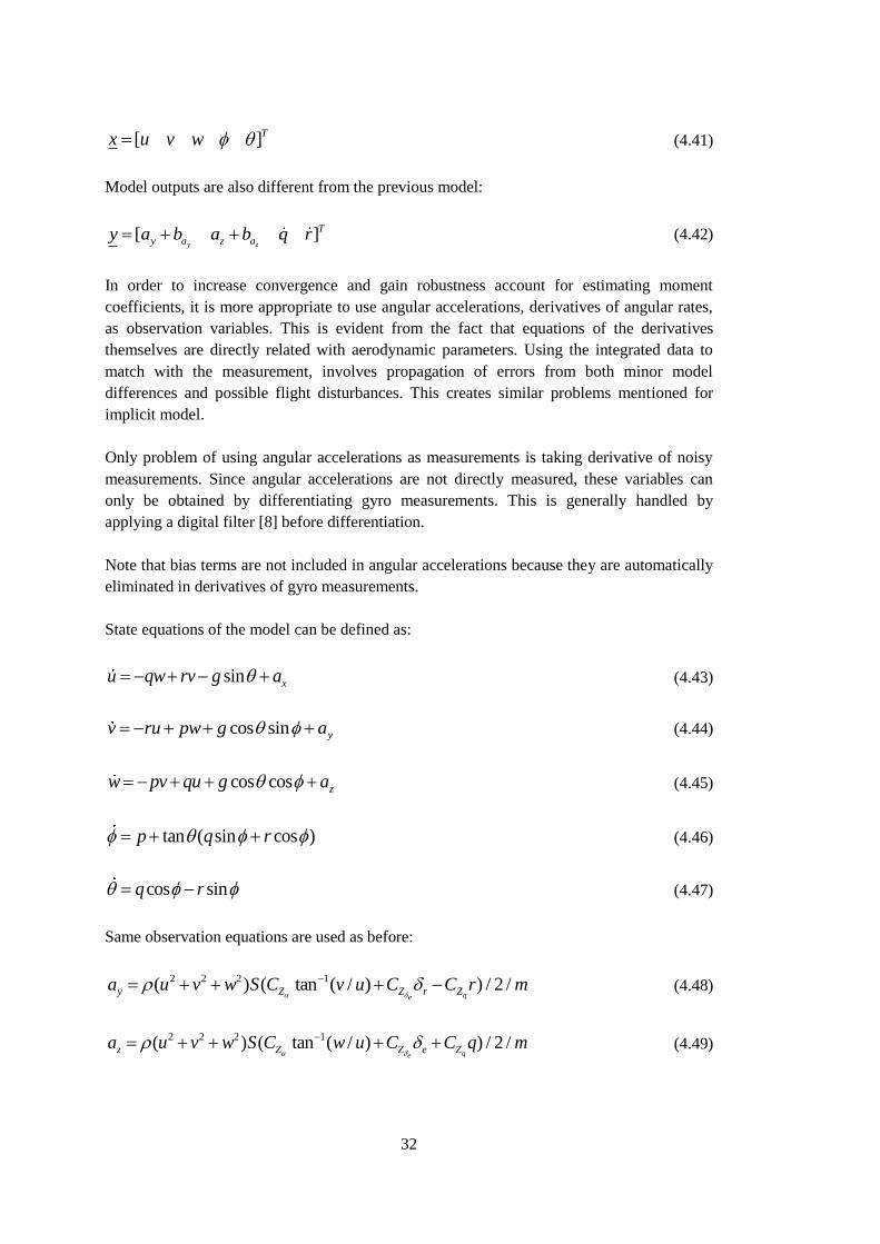
[ ]Tx u v w (4.41)

Model outputs are also different from the previous model:

[ ]y z

T

y a z ay a b a b q r (4.42)

In order to increase convergence and gain robustness account for estimating moment

coefficients, it is more appropriate to use angular accelerations, derivatives of angular rates,

as observation variables. This is evident from the fact that equations of the derivatives

themselves are directly related with aerodynamic parameters. Using the integrated data to

match with the measurement, involves propagation of errors from both minor model

differences and possible flight disturbances. This creates similar problems mentioned for

implicit model.

Only problem of using angular accelerations as measurements is taking derivative of noisy

measurements. Since angular accelerations are not directly measured, these variables can

only be obtained by differentiating gyro measurements. This is generally handled by

applying a digital filter [8] before differentiation.

Note that bias terms are not included in angular accelerations because they are automatically

eliminated in derivatives of gyro measurements.

State equations of the model can be defined as:

sin xu qw rv g a (4.43)

cos sin yv ru pw g a (4.44)

cos cos zw pv qu g a (4.45)

tan ( sin cos )p q r (4.46)

cos sinq r (4.47)

Same observation equations are used as before:

2 2 2 1( ) ( tan ( / ) ) / 2 /

qeZy Z r Za u v w S C v u C C r m

(4.48)

2 2 2 1( ) ( tan ( / ) ) / 2 /

qez Z Z e Za u v w S C w u C C q m

(4.49)

33

2 2 2 1

(1 / )

( ) ( tan ( / ) ) / 2 /qe

M M e M

x y

y

q J J pr

u v w Sl C w u C C q J

(4.50)

2 2 2 1

( / 1)

( ) ( tan ( / ) ) / 2 /qe

M

y

M r M

x

y

r J J pq

u v w Sl C v u C C r J

(4.51)

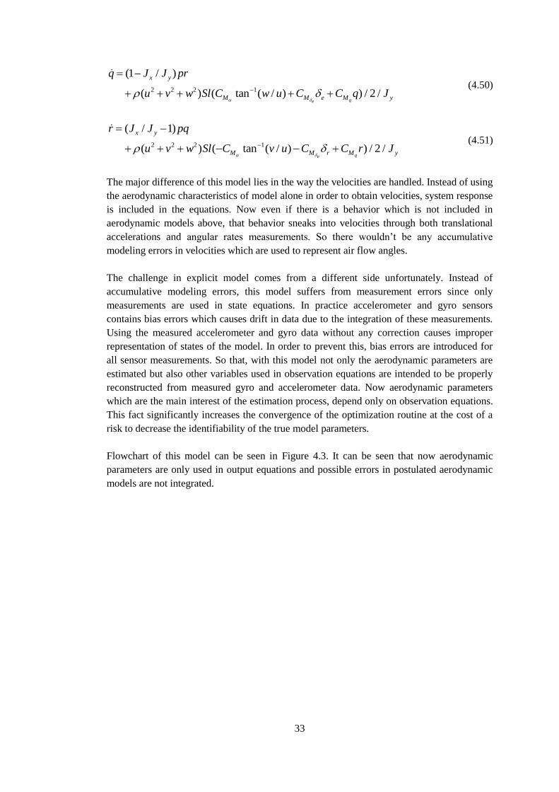
The major difference of this model lies in the way the velocities are handled. Instead of using

the aerodynamic characteristics of model alone in order to obtain velocities, system response

is included in the equations. Now even if there is a behavior which is not included in

aerodynamic models above, that behavior sneaks into velocities through both translational

accelerations and angular rates measurements. So there wouldn’t be any accumulative

modeling errors in velocities which are used to represent air flow angles.

The challenge in explicit model comes from a different side unfortunately. Instead of

accumulative modeling errors, this model suffers from measurement errors since only

measurements are used in state equations. In practice accelerometer and gyro sensors

contains bias errors which causes drift in data due to the integration of these measurements.

Using the measured accelerometer and gyro data without any correction causes improper

representation of states of the model. In order to prevent this, bias errors are introduced for

all sensor measurements. So that, with this model not only the aerodynamic parameters are

estimated but also other variables used in observation equations are intended to be properly

reconstructed from measured gyro and accelerometer data. Now aerodynamic parameters

which are the main interest of the estimation process, depend only on observation equations.

This fact significantly increases the convergence of the optimization routine at the cost of a

risk to decrease the identifiability of the true model parameters.

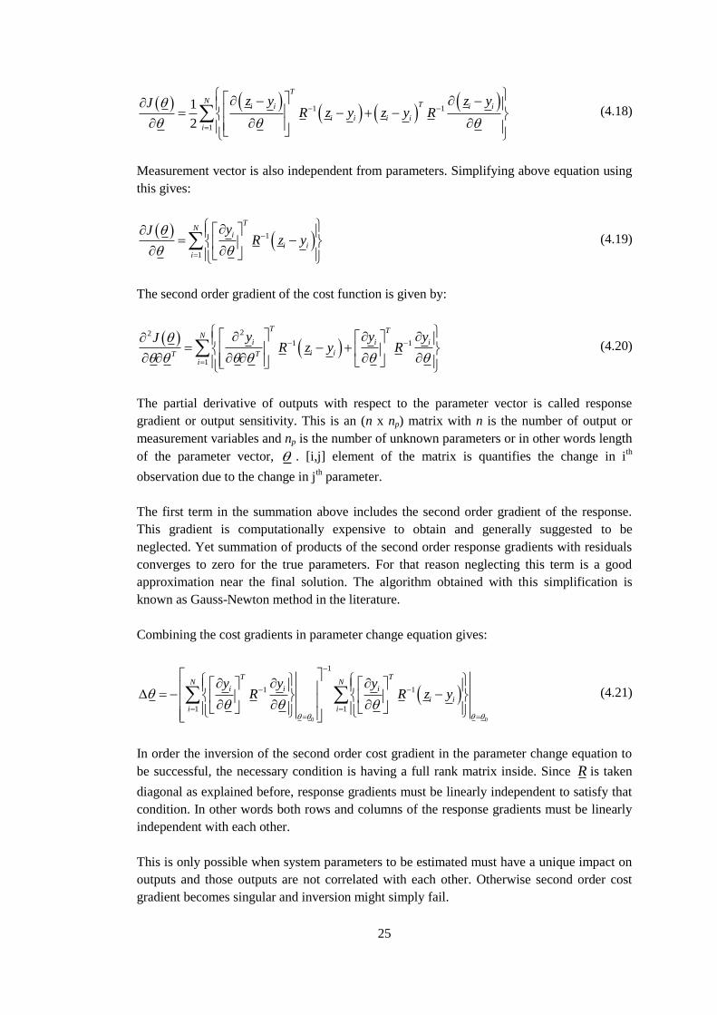
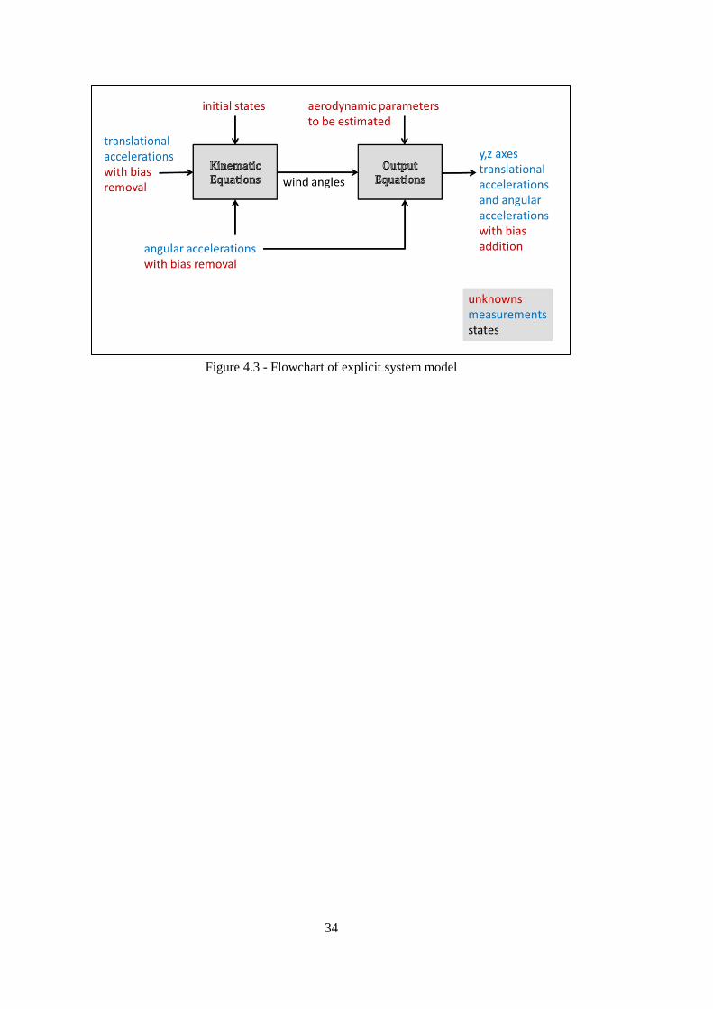
Flowchart of this model can be seen in Figure 4.3. It can be seen that now aerodynamic

parameters are only used in output equations and possible errors in postulated aerodynamic

models are not integrated.

34

Figure 4.3 - Flowchart of explicit system model

35

CHAPTER 5

5. ESTIMATION RESULTS

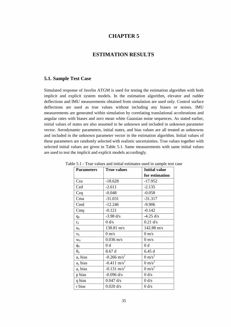
5.1. Sample Test Case

Simulated response of Javelin ATGM is used for testing the estimation algorithm with both

implicit and explicit system models. In the estimation algorithm, elevator and rudder

deflections and IMU measurements obtained from simulation are used only. Control surface

deflections are used as true values without including any biases or noises. IMU

measurements are generated within simulation by correlating translational accelerations and

angular rates with biases and zero mean white Gaussian noise sequences. As stated earlier,

initial values of states are also assumed to be unknown and included in unknown parameter

vector. Aerodynamic parameters, initial states, and bias values are all treated as unknowns

and included in the unknown parameter vector in the estimation algorithm. Initial values of

these parameters are randomly selected with realistic uncertainties. True values together with

selected initial values are given in Table 5.1. Same measurements with same initial values

are used to test the implicit and explicit models accordingly.

Table 5.1 - True values and initial estimates used in sample test case

Parameters True values Initial value

for estimation

Cza -18.628 -17.952

Czd -2.611 -2.135

Czq -0.048 -0.058

Cma -31.031 -31.317

Cmd -12.246 -9.906

Cmq -0.121 -0.142

q0 -3.98 d/s -4.25 d/s

r0 0 d/s 0.21 d/s

u0 138.81 m/s 142.88 m/s

v0 0 m/s 0 m/s

w0 0.036 m/s 0 m/s

ϕ0 0 d 0 d

θ0 8.67 d 6.45 d

ax bias -0.266 m/s2 0 m/s

2

ay bias -0.411 m/s2 0 m/s

2

az bias -0.131 m/s2 0 m/s

2

p bias -0.096 d/s 0 d/s

q bias 0.047 d/s 0 d/s

r bias 0.020 d/s 0 d/s

36

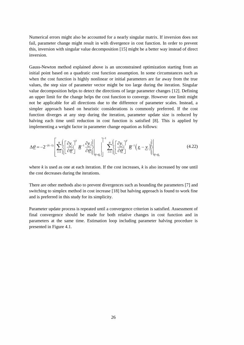
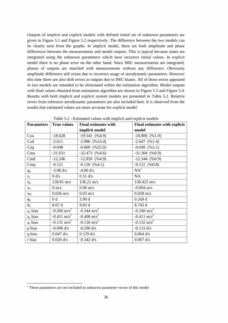
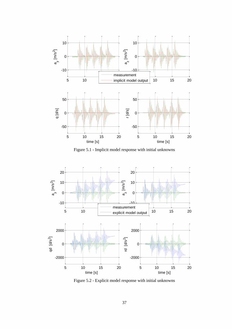
Outputs of implicit and explicit models with defined initial set of unknown parameters are

given in Figure 5.1 and Figure 5.2 respectively. The difference between the two models can

be clearly seen from the graphs. In implicit model, there are both amplitude and phase

differences between the measurements and model outputs. This is typical because states are

integrated using the unknown parameters which have incorrect initial values. In explicit

model there is no phase error on the other hand. Since IMU measurements are integrated,

phases of outputs are matched with measurements without any difference. Obviously

amplitude difference still exists due to incorrect usage of aerodynamic parameters. However

this time there are also drift errors in outputs due to IMU biases. All of those errors appeared

in two models are intended to be eliminated within the estimation algorithm. Model outputs

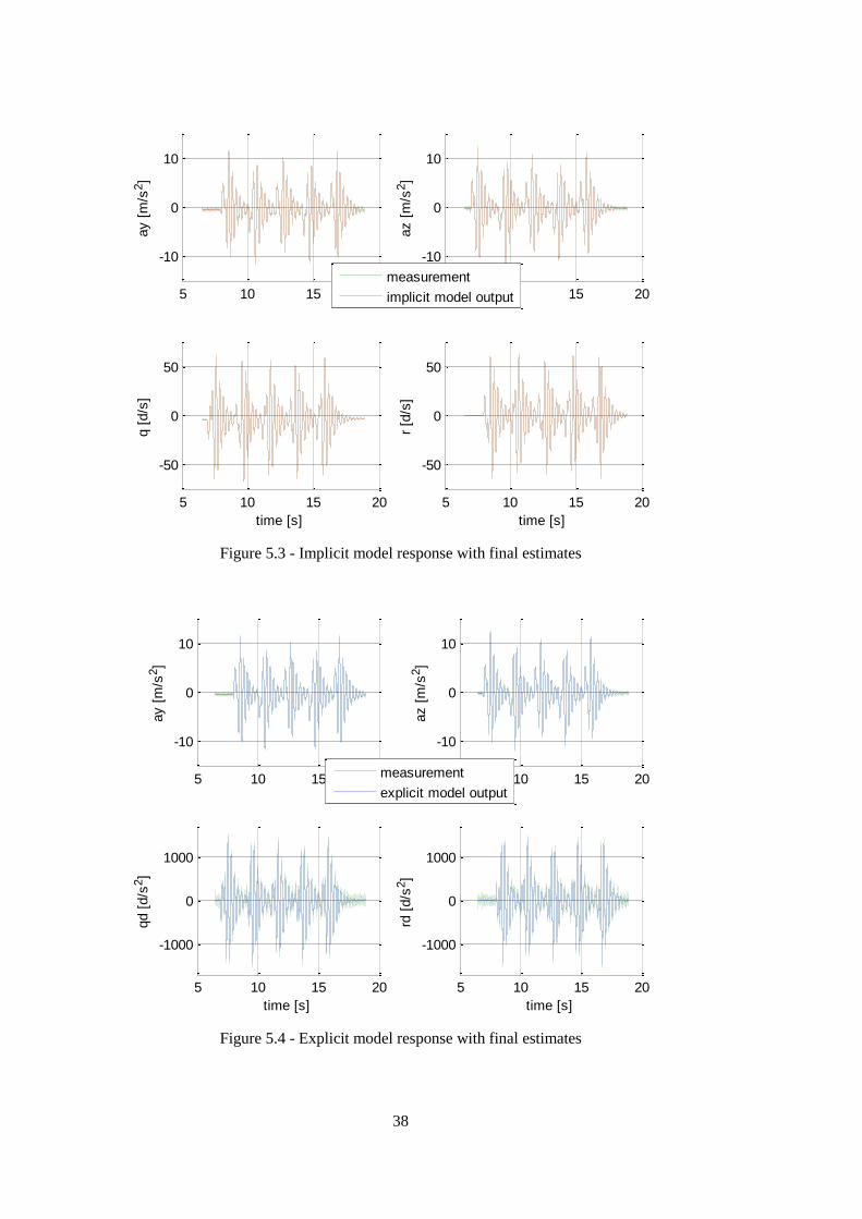
with final values obtained from estimation algorithm are shown in Figure 5.3 and Figure 5.4.

Results with both implicit and explicit system models are presented in Table 5.2. Relative

errors from reference aerodynamic parameters are also included here. It is observed from the

results that estimated values are more accurate for explicit model.

Table 5.2 - Estimated values with implicit and explicit models

Parameters True values Final estimates with

implicit model

Final estimates with explicit

model

Cza -18.628 -19.541 (%4.9) -18.806 (%1.0)

Czd -2.611 -2.986 (%14.4) -2.647 (%1.4)

Czq -0.048 -0.060 (%25.0) -0.049 (%2.1)

Cma -31.031 -32.473 (%4.6) -31.304 (%0.9)

Cmd -12.246 -12.850 (%4.9) -12.344 (%0.9)

Cmq -0.121 -0.126 (%4.1) -0.122 (%0.8)

q0 -3.98 d/s -4.00 d/s NAa

r0 0 d/s 0.31 d/s NA

u0 138.81 m/s 136.21 m/s 138.425 m/s

v0 0 m/s 0.00 m/s -0.004 m/s

w0 0.036 m/s 0.03 m/s 0.028 m/s

ϕ0 0 d 3.90 d 0.169 d

θ0 8.67 d 9.83 d 8.743 d

ax bias -0.266 m/s2 -0.344 m/s

2 -0.240 m/s

2

ay bias -0.411 m/s2 -0.408 m/s

2 -0.411 m/s

2

az bias -0.131 m/s2 -0.136 m/s

2 -0.132 m/s

2

p bias -0.096 d/s -0.290 d/s -0.133 d/s

q bias 0.047 d/s 0.129 d/s 0.064 d/s

r bias 0.020 d/s -0.342 d/s 0.007 d/s

a These parameters are not included in unknown parameter vector of this model

37

Figure 5.1 - Implicit model response with initial unknowns

Figure 5.2 - Explicit model response with initial unknowns

5 10 15 20

-10

0

10

ay [

m/s

2]

5 10 15 20

-10

0

10

az [

m/s

2]

5 10 15 20

-50

0

50

time [s]

q [

d/s

]

5 10 15 20

-50

0

50

time [s]

r [d

/s]

measurement

implicit model output

5 10 15 20

-10

0

10

20

ay [

m/s

2]

5 10 15 20

-10

0

10

20

az [

m/s

2]

5 10 15 20

-2000

0

2000

time [s]

qd

[d/s

2]

5 10 15 20

-2000

0

2000

time [s]

rd

[d/s

2]

measurement

explicit model output

38

Figure 5.3 - Implicit model response with final estimates

Figure 5.4 - Explicit model response with final estimates

5 10 15 20

-10

0

10

ay [

m/s

2]

5 10 15 20

-10

0

10

az [

m/s

2]

5 10 15 20

-50

0

50

time [s]

q [

d/s

]

5 10 15 20

-50

0

50

time [s]

r [d

/s]

measurement

implicit model output

5 10 15 20

-10

0

10

ay [

m/s

2]

5 10 15 20

-10

0

10

az [

m/s

2]

5 10 15 20

-1000

0

1000

time [s]

qd [

d/s

2]

5 10 15 20

-1000

0

1000

time [s]

rd [

d/s

2]

measurement

explicit model output

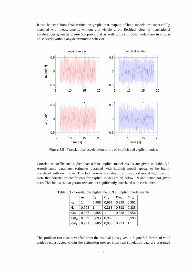
39

It can be seen from final estimation graphs that outputs of both models are successfully

matched with measurements without any visible error. Residual plots of translational

accelerations given in Figure 5.5 prove that as well. Errors in both models are in similar

noise levels without any deterministic behavior.

Figure 5.5 - Translational acceleration errors of implicit and explicit models

Correlation coefficients higher than 0.9 in implicit model results are given in Table 5.3.

Aerodynamic parameter estimates obtained with implicit model appear to be highly

correlated with each other. This fact reduces the reliability of implicit model significantly.

Note that correlation coefficients for explicit model are all below 0.9 and hence not given

here. This indicates that parameters are not significantly correlated with each other.

Table 5.3 - Correlations higher than 0.9 in implicit model results

u0 θ0 Czα Cmα Cmδ

u0 1 0,908 0,967 0,999 0,992

θ0 0,908 1 0,865 0,893 0,885

Czα 0,967 0,865 1 0,968 0,956

Cmα 0,999 0,893 0,968 1 0,993

Cmδ 0,992 0,885 0,956 0,993 1

This problem can also be verified from the residual plots given in Figure 5.6. Errors of wind

angles reconstructed within the estimation process from real simulation data are presented

5 10 15 20

-0.5

0

0.5

ay [

m/s

2]

implicit model

5 10 15 20

-0.5

0

0.5

explicit model

5 10 15 20

-0.5

0

0.5

az [

m/s

2]

time [s]

5 10 15 20

-0.5

0

0.5

time [s]

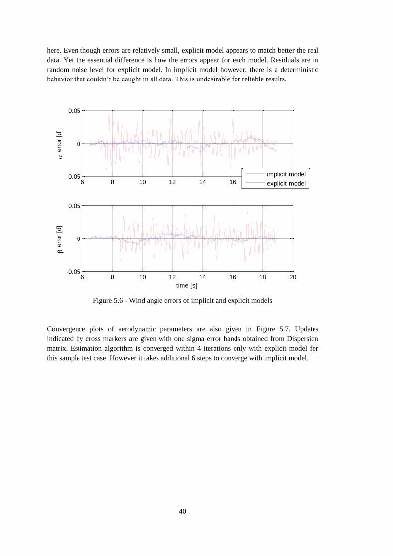
40

here. Even though errors are relatively small, explicit model appears to match better the real

data. Yet the essential difference is how the errors appear for each model. Residuals are in

random noise level for explicit model. In implicit model however, there is a deterministic

behavior that couldn’t be caught in all data. This is undesirable for reliable results.

Figure 5.6 - Wind angle errors of implicit and explicit models

Convergence plots of aerodynamic parameters are also given in Figure 5.7. Updates

indicated by cross markers are given with one sigma error bands obtained from Dispersion

matrix. Estimation algorithm is converged within 4 iterations only with explicit model for

this sample test case. However it takes additional 6 steps to converge with implicit model.

6 8 10 12 14 16 18 20-0.05

0

0.05

e

rror

[d]

6 8 10 12 14 16 18 20-0.05

0

0.05

time [s]

e

rror

[d]

implicit model

explicit model

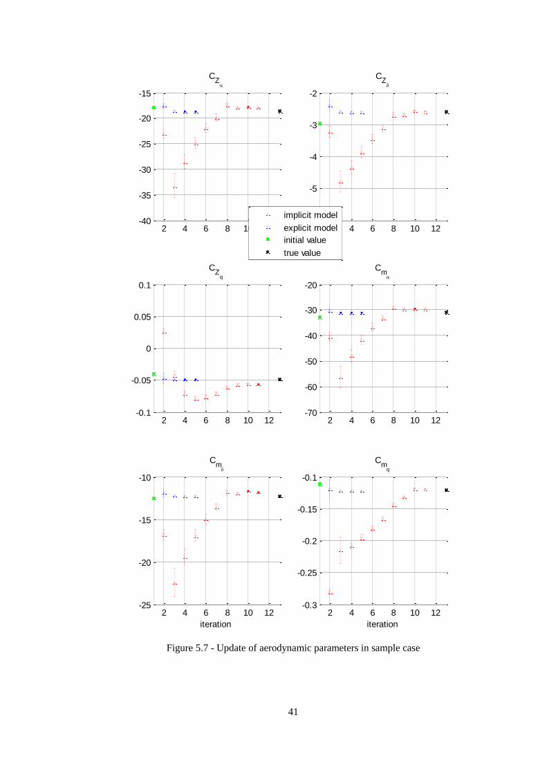
41

Figure 5.7 - Update of aerodynamic parameters in sample case

2 4 6 8 10 12-40

-35

-30

-25

-20

-15

CZ

2 4 6 8 10 12-6

-5

-4

-3

-2

CZ

2 4 6 8 10 12-0.1

-0.05

0

0.05

0.1

CZ

q

2 4 6 8 10 12-70

-60

-50

-40

-30

-20

Cm

2 4 6 8 10 12-25

-20

-15

-10

Cm

iteration

2 4 6 8 10 12-0.3

-0.25

-0.2

-0.15

-0.1

Cm

q

iteration

implicit model

explicit model

initial value

true value

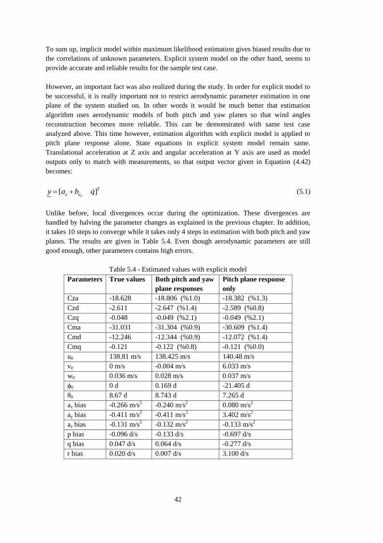
42

To sum up, implicit model within maximum likelihood estimation gives biased results due to

the correlations of unknown parameters. Explicit system model on the other hand, seems to

provide accurate and reliable results for the sample test case.

However, an important fact was also realized during the study. In order for explicit model to

be successful, it is really important not to restrict aerodynamic parameter estimation in one

plane of the system studied on. In other words it would be much better that estimation

algorithm uses aerodynamic models of both pitch and yaw planes so that wind angles

reconstruction becomes more reliable. This can be demonstrated with same test case

analyzed above. This time however, estimation algorithm with explicit model is applied to

pitch plane response alone. State equations in explicit system model remain same.

Translational acceleration at Z axis and angular acceleration at Y axis are used as model

outputs only to match with measurements, so that output vector given in Equation (4.42)

becomes:

[ ]z

T

z ay a b q (5.1)

Unlike before, local divergences occur during the optimization. These divergences are

handled by halving the parameter changes as explained in the previous chapter. In addition,

it takes 10 steps to converge while it takes only 4 steps in estimation with both pitch and yaw

planes. The results are given in Table 5.4. Even though aerodynamic parameters are still

good enough, other parameters contains high errors.

Table 5.4 - Estimated values with explicit model

Parameters True values Both pitch and yaw

plane responses

Pitch plane response

only

Cza -18.628 -18.806 (%1.0) -18.382 (%1.3)

Czd -2.611 -2.647 (%1.4) -2.589 (%0.8)

Czq -0.048 -0.049 (%2.1) -0.049 (%2.1)

Cma -31.031 -31.304 (%0.9) -30.609 (%1.4)

Cmd -12.246 -12.344 (%0.9) -12.072 (%1.4)

Cmq -0.121 -0.122 (%0.8) -0.121 (%0.0)

u0 138.81 m/s 138.425 m/s 140.48 m/s

v0 0 m/s -0.004 m/s 6.033 m/s

w0 0.036 m/s 0.028 m/s 0.037 m/s

ϕ0 0 d 0.169 d -21.405 d

θ0 8.67 d 8.743 d 7.265 d

ax bias -0.266 m/s2 -0.240 m/s

2 0.080 m/s

2

ay bias -0.411 m/s2 -0.411 m/s

2 3.402 m/s

2

az bias -0.131 m/s2 -0.132 m/s

2 -0.133 m/s

2

p bias -0.096 d/s -0.133 d/s -0.697 d/s

q bias 0.047 d/s 0.064 d/s -0.277 d/s

r bias 0.020 d/s 0.007 d/s 3.100 d/s

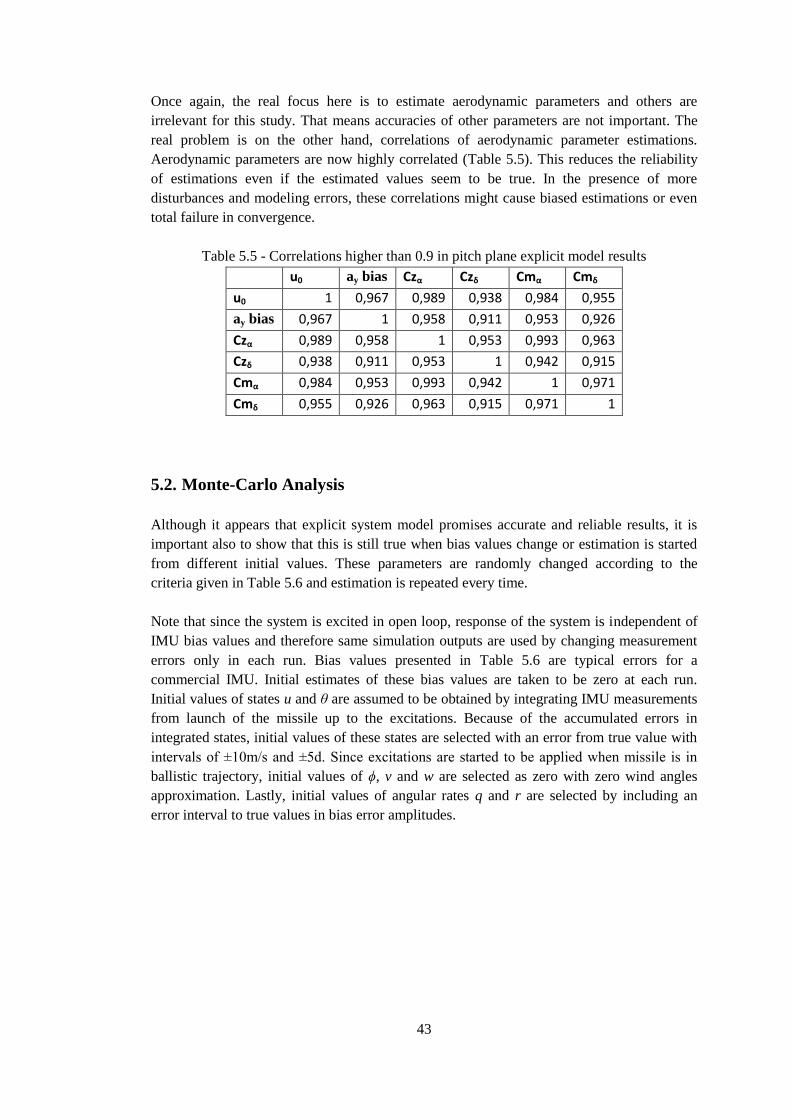
43

Once again, the real focus here is to estimate aerodynamic parameters and others are

irrelevant for this study. That means accuracies of other parameters are not important. The

real problem is on the other hand, correlations of aerodynamic parameter estimations.

Aerodynamic parameters are now highly correlated (Table 5.5). This reduces the reliability

of estimations even if the estimated values seem to be true. In the presence of more

disturbances and modeling errors, these correlations might cause biased estimations or even

total failure in convergence.

Table 5.5 - Correlations higher than 0.9 in pitch plane explicit model results

u0 ay bias Czα Czδ Cmα Cmδ

u0 1 0,967 0,989 0,938 0,984 0,955

ay bias 0,967 1 0,958 0,911 0,953 0,926

Czα 0,989 0,958 1 0,953 0,993 0,963

Czδ 0,938 0,911 0,953 1 0,942 0,915

Cmα 0,984 0,953 0,993 0,942 1 0,971

Cmδ 0,955 0,926 0,963 0,915 0,971 1

5.2. Monte-Carlo Analysis

Although it appears that explicit system model promises accurate and reliable results, it is

important also to show that this is still true when bias values change or estimation is started

from different initial values. These parameters are randomly changed according to the

criteria given in Table 5.6 and estimation is repeated every time.

Note that since the system is excited in open loop, response of the system is independent of

IMU bias values and therefore same simulation outputs are used by changing measurement

errors only in each run. Bias values presented in Table 5.6 are typical errors for a

commercial IMU. Initial estimates of these bias values are taken to be zero at each run.

Initial values of states u and θ are assumed to be obtained by integrating IMU measurements

from launch of the missile up to the excitations. Because of the accumulated errors in

integrated states, initial values of these states are selected with an error from true value with

intervals of ±10m/s and ±5d. Since excitations are started to be applied when missile is in

ballistic trajectory, initial values of ϕ, v and w are selected as zero with zero wind angles

approximation. Lastly, initial values of angular rates q and r are selected by including an

error interval to true values in bias error amplitudes.

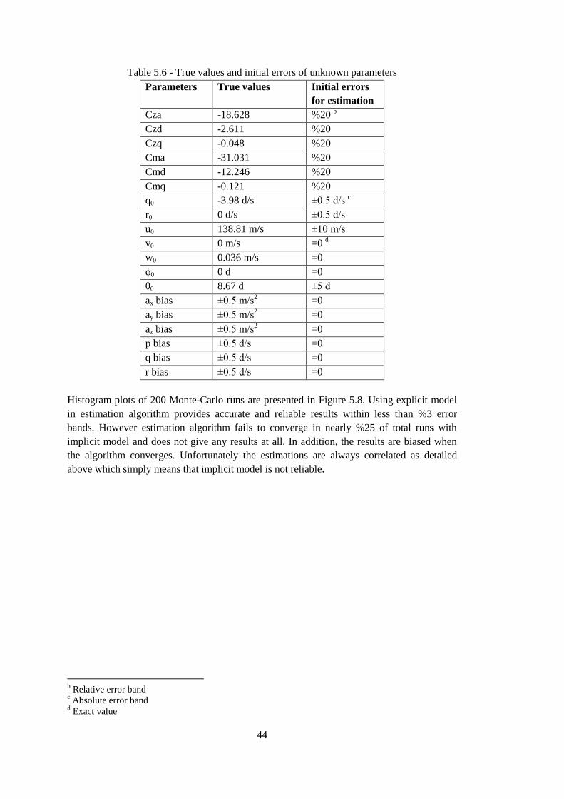
44

Table 5.6 - True values and initial errors of unknown parameters

Parameters True values Initial errors

for estimation

Cza -18.628 %20 b

Czd -2.611 %20

Czq -0.048 %20

Cma -31.031 %20

Cmd -12.246 %20

Cmq -0.121 %20

q0 -3.98 d/s ±0.5 d/s c

r0 0 d/s ±0.5 d/s

u0 138.81 m/s ±10 m/s

v0 0 m/s =0 d

w0 0.036 m/s =0

ϕ0 0 d =0

θ0 8.67 d ±5 d

ax bias ±0.5 m/s2 =0

ay bias ±0.5 m/s2 =0

az bias ±0.5 m/s2 =0

p bias ±0.5 d/s =0

q bias ±0.5 d/s =0

r bias ±0.5 d/s =0

Histogram plots of 200 Monte-Carlo runs are presented in Figure 5.8. Using explicit model

in estimation algorithm provides accurate and reliable results within less than %3 error

bands. However estimation algorithm fails to converge in nearly %25 of total runs with

implicit model and does not give any results at all. In addition, the results are biased when

the algorithm converges. Unfortunately the estimations are always correlated as detailed

above which simply means that implicit model is not reliable.

b Relative error band

c Absolute error band

d Exact value

45

Figure 5.8 - Monte-Carlo results of implicit and explicit models

5.3. Real Flight Test

-19.8 -19.6 -19.4 -19.2 -19 -18.8 -18.6 -18.4 -18.2 -18 -17.80

50

CZ

-3.1 -3 -2.9 -2.8 -2.7 -2.6 -2.5 -2.40

50

CZ

-0.062 -0.06 -0.058 -0.056 -0.054 -0.052 -0.05 -0.048 -0.0460

50

CZ

q

-33 -32.5 -32 -31.5 -31 -30.5 -300

50

Cm

-13 -12.8 -12.6 -12.4 -12.2 -12 -11.80

50

Cm

-0.127 -0.126 -0.125 -0.124 -0.123 -0.122 -0.121 -0.12 -0.119 -0.118 -0.1170

50

Cm

q

implicit model

explicit model

true value

%3 error bands

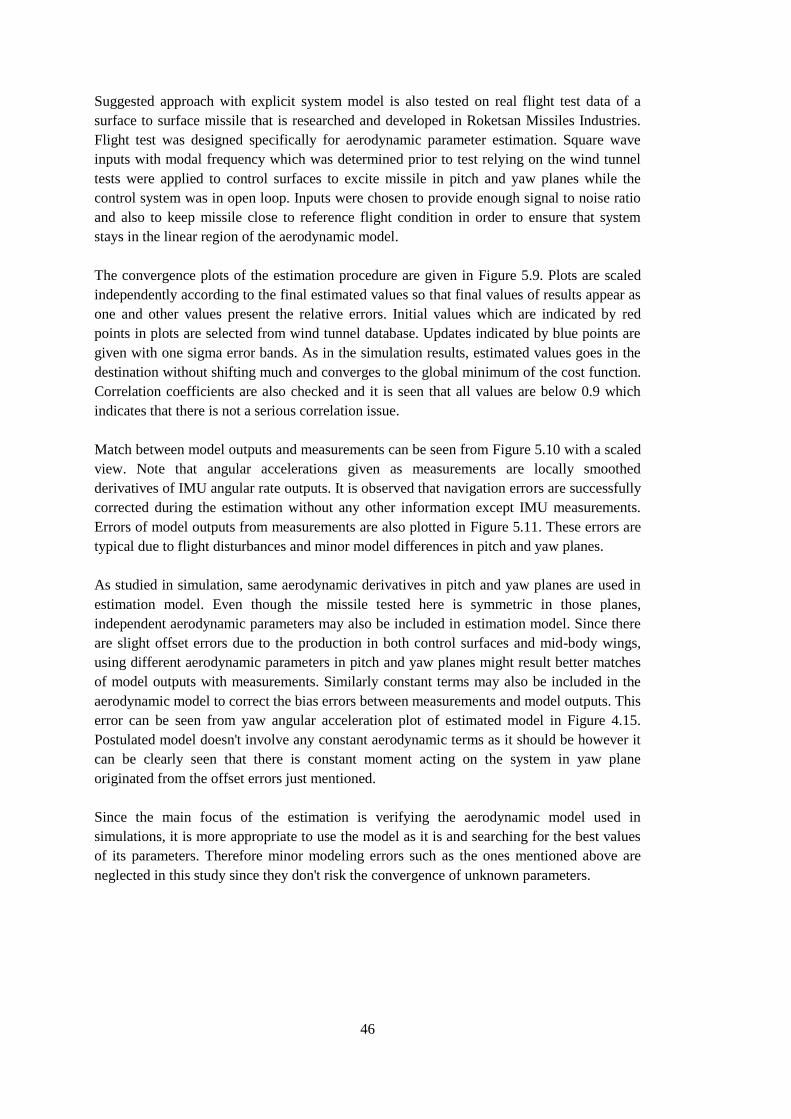
46

Suggested approach with explicit system model is also tested on real flight test data of a

surface to surface missile that is researched and developed in Roketsan Missiles Industries.

Flight test was designed specifically for aerodynamic parameter estimation. Square wave

inputs with modal frequency which was determined prior to test relying on the wind tunnel

tests were applied to control surfaces to excite missile in pitch and yaw planes while the

control system was in open loop. Inputs were chosen to provide enough signal to noise ratio

and also to keep missile close to reference flight condition in order to ensure that system

stays in the linear region of the aerodynamic model.

The convergence plots of the estimation procedure are given in Figure 5.9. Plots are scaled

independently according to the final estimated values so that final values of results appear as

one and other values present the relative errors. Initial values which are indicated by red

points in plots are selected from wind tunnel database. Updates indicated by blue points are

given with one sigma error bands. As in the simulation results, estimated values goes in the

destination without shifting much and converges to the global minimum of the cost function.

Correlation coefficients are also checked and it is seen that all values are below 0.9 which

indicates that there is not a serious correlation issue.

Match between model outputs and measurements can be seen from Figure 5.10 with a scaled

view. Note that angular accelerations given as measurements are locally smoothed

derivatives of IMU angular rate outputs. It is observed that navigation errors are successfully

corrected during the estimation without any other information except IMU measurements.

Errors of model outputs from measurements are also plotted in Figure 5.11. These errors are

typical due to flight disturbances and minor model differences in pitch and yaw planes.

As studied in simulation, same aerodynamic derivatives in pitch and yaw planes are used in

estimation model. Even though the missile tested here is symmetric in those planes,

independent aerodynamic parameters may also be included in estimation model. Since there

are slight offset errors due to the production in both control surfaces and mid-body wings,

using different aerodynamic parameters in pitch and yaw planes might result better matches

of model outputs with measurements. Similarly constant terms may also be included in the

aerodynamic model to correct the bias errors between measurements and model outputs. This

error can be seen from yaw angular acceleration plot of estimated model in Figure 4.15.

Postulated model doesn't involve any constant aerodynamic terms as it should be however it

can be clearly seen that there is constant moment acting on the system in yaw plane

originated from the offset errors just mentioned.

Since the main focus of the estimation is verifying the aerodynamic model used in

simulations, it is more appropriate to use the model as it is and searching for the best values

of its parameters. Therefore minor modeling errors such as the ones mentioned above are

neglected in this study since they don't risk the convergence of unknown parameters.

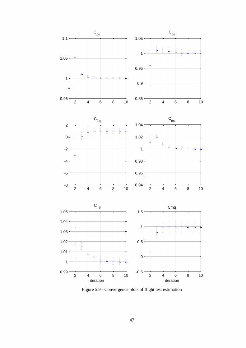
47

Figure 5.9 - Convergence plots of flight test estimation

2 4 6 8 100.95

1

1.05

1.1

CZ

2 4 6 8 100.85

0.9

0.95

1

1.05

CZ

2 4 6 8 10-8

-6

-4

-2

0

2

CZq

2 4 6 8 100.94

0.96

0.98

1

1.02

1.04

Cm

2 4 6 8 100.99

1

1.01

1.02

1.03

1.04

1.05

Cm

iteration

2 4 6 8 10-0.5

0

0.5

1

1.5Cmq

iteration

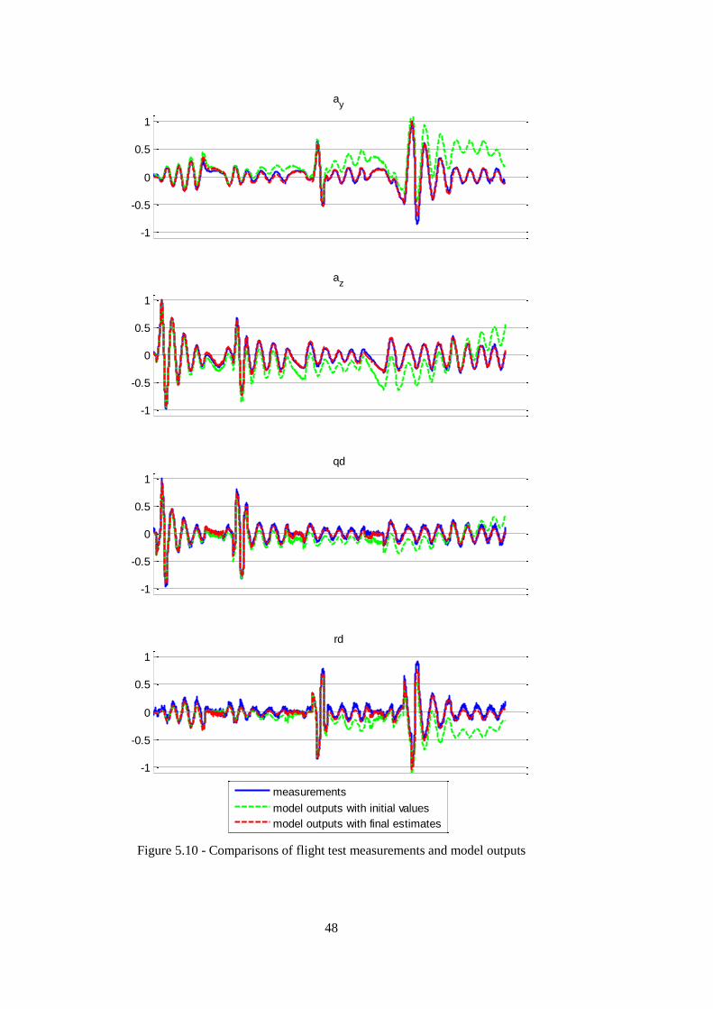
48

Figure 5.10 - Comparisons of flight test measurements and model outputs

-1

-0.5

0

0.5

1

ay

-1

-0.5

0

0.5

1

az

-1

-0.5

0

0.5

1

qd

-1

-0.5

0

0.5

1

rd

measurements

model outputs with initial values

model outputs with final estimates

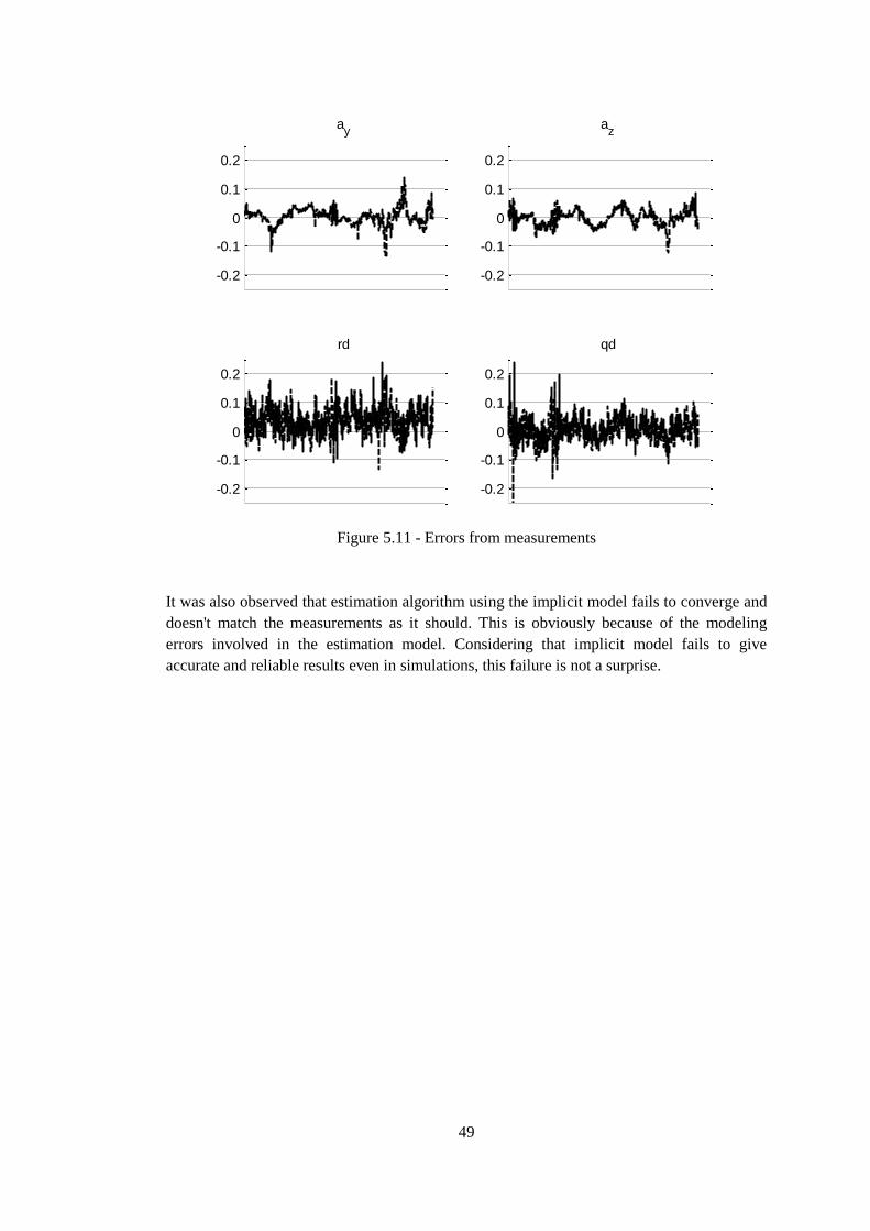
49

Figure 5.11 - Errors from measurements

It was also observed that estimation algorithm using the implicit model fails to converge and

doesn't match the measurements as it should. This is obviously because of the modeling

errors involved in the estimation model. Considering that implicit model fails to give

accurate and reliable results even in simulations, this failure is not a surprise.

-0.2

-0.1

0

0.1

0.2

ay

-0.2

-0.1

0

0.1

0.2

az

-0.2

-0.1

0

0.1

0.2

qd

-0.2

-0.1

0

0.1

0.2

rd

50

51

CHAPTER 6

6. CONCLUSIONS

Estimating aerodynamic parameters of flight vehicles from real tests has always been a great

interest. There are numerous studies that focuses on this subject in the literature. However

only a limited number of references exist for missiles compared to aircraft. The natural

problem that arises while estimating aerodynamic parameters of missiles is lack of wind

angles measurements. This problem is usually handled by calculating wind angles from

flight test measurements during post processing prior to the estimation study. When only

IMU measurements are available for the response of the system, post processed data is

subjected to drift errors because of biased measurements. This brings a need of alternative

approach for estimating aerodynamic parameters when wind angles measurements are not

available.

In this thesis aerodynamic parameter estimation of a missile in the absence of wind angles

measurements is studied in detail. Output error method is utilized for the estimation of

aerodynamic parameters. Two different system models are proposed to be used in this

method. Without using any post process calculations, wind angles are determined within the

estimation. As for the measurements; translational accelerations, angular rates and control

surface deflections are used.

First model which is named implicit model uses the equations of motion of the system as

state equations. In other words unknown aerodynamic parameters are used in state equations.

Outputs of the model are selected as translational accelerations and angular rates. Using this

model in output-error method is like simulating the response of the system with current

values of unknown parameters during the iterations. In fact output-error method is generally

preferred to be able to use the aerodynamic parameters in state equations for more reliable

results [4]. Therefore implicit system model is the very first approach that naturally comes to

mind.

Unfortunately, it is demonstrated with simulated data that aerodynamic parameters are

simply not observable with this approach. Estimation results appear –when algorithm

converges– to be biased and highly correlated with each other. This is a typical problem

when the model structure includes either too many terms or too few terms relative to the

information content in the data [17]. In this case there are too many unknowns with limited

information about response. This approach is also tested with data of a real flight test which

is designed specifically for estimation. As a proof of simulation study, estimation algorithm

doesn’t converge to any results in real flight test. If wind angles measurements were

available, this might have not happened [12] or alternatively the problem could be easily

eliminated by using those measurements as inputs in state equations [8].

52

In the second system model which is named explicit model, state equations are made free of

unknown system characteristics. Translational accelerations and angular accelerations, which

are obtained from locally smoothed derivatives of angular rates, are used as inputs and state

equations are built from kinematic equations. Bias values of measurements are used as

unknowns in state equations in order to be able to eliminate drift errors. Aerodynamic

parameters are now included in output equations only. Thus this approach can be thought as

a nonlinear equation-error method instead. If translational accelerations and angular rates

measurements were somehow bias free, the easiest way of estimating aerodynamic

parameters would be integrating those measurements to obtain all the states (with no wind

assumption) and then applying a least square fit which is known as equation-error method.

However measurement bias cause accumulated errors when integrated, which cannot be

corrected easily when the exact bias value is not known. Using proposed explicit system

model with output-error method provides a way of correcting those errors iteratively. This is

online reconstruction of states during the estimation. Then in the last step, method gives the

maximum likelihood estimates using reconstructed states, which are essentially the same as

least square estimates [8].

Trials with simulation data show that second approach, estimation with explicit system

model, provides reliable and accurate results. In addition, algorithm is applied to real flight

test data with success. The results of this study demonstrate that with this suggested

approach aerodynamic parameter estimation can be accurately done without measurements

of wind angles. However an important fact must be emphasized here again. This approach is

meant to work only when the system is excited in both pitch and yaw planes. Otherwise

online reconstruction mentioned above fails to give accurate results. This is demonstrated

with simulated data by applying the estimation in pitch plane only.

Studied missile in this thesis is symmetric in pitch and yaw planes therefore it has the same

aerodynamic model in both planes. This is clearly a benefit for estimation with limited

measurements. Yet there is opportunity to apply the suggested approach to asymmetric

systems. In Appendix A, suggested approach is tested with real flight data of a research

aircraft without going too much detail. It is apparent from the results that it might be possible

to accurately estimate aerodynamic parameters of aircraft with this approach suggested here,

as well.

The first assumption made in this study is no wind condition. Even though wind is excluded

in this study, suggested approach would still work in the case of a steady wind. Including

additional constant terms in aerodynamic model might help algorithm to model the effect of

wind in these terms. Nevertheless, this should be tested in detail as a future work. In

addition, an effort should be directed to apply this approach with a state filter to eliminate

flight disturbances. This would be necessary to obtain more accurate estimations in the case

of turbulent atmosphere.

53

REFERENCES

[1] Aydın G., “Aerodynamic Parameter Estimation of A Missile in Closed Loop Control

and Validation with Flight Data”, M.Sc. Thesis, METU, 2012.

[2] W. B. Blake., “Missile Datcom User’s Manual - 1997 Fortran 90 Revision”, Wright-

Patterson Air Force Base, 1998.

[3] DLR, http://www.dlr.de/dlr/en/desktopdefault.aspx/tabid-10644/#gallery/6043, last

visited on July 2013

[4] Hamel P. G., Jategaonkar R. V., “Evolution of Flight Vehicle System Identification",

AIAA, Journal of Aircraft, Vol. 33, No. 1, 1996.

[5] Harris J., Slegers N., “Performance of A Fire-and-Forget Anti-Tank Missile with A

Damaged Wing”, ScienceDirect, Mathematical and Computer Modeling 50, 292-305,

2009.

[6] Lockheed Martin,

http://www.lockheedmartin.com/content/dam/lockheed/data/mfc/pc/javelin/mfc-

javelin-pc.pdf, last visited on July 2013

[7] Jategaonkar R. V., “Bounded-Variable Gauss–Newton Algorithm for Aircraft

Parameter Estimation” ,AIAA, Journal of Aircraft, Vol. 37, No. 4, 2000.

[8] Jategaonkar R. V., “Flight Vehicle System Identification: A Time Domain

Methodology”, AIAA, Progress in Astronautics and Aeronautics Volume 216, 2006.

[9] Jategaonkar R. V., “Identification of the Aerodynamic Model of the DLR Research

Aircraft ATTAS from Flight Test Data”, DLR-FB 90-40, 1990.

[10] Jategaonkar, R. V, "A Comparison of Output Error and FilterError Methods from

Aircraft Parameter Estimation Results", DLR-Mitt.93-14, pp. 63-87, 1993.

[11] Kailath T., “A General Likelihood Ratio Formula for Random Signals in Gaussian

Noise", IEEE Transactions on Information Theory, Vol IT 15, No.3,1969

[12] Klein V., Morelli E. A., “Aircraft System Identification Theory and Practice”, AIAA

Education Series, 2006.

[13] Kutluay Ü., “Aerodynamic Parameter Estimation Using Flight Test Data”, Phd Thesis,

METU, 2011.

54

[14] Lyons J., Long D., Chait R., “Critical Technology Events in the Development of the

Stinger and Javelin Missile Systems”, Center for Technology and National Security

Policy, National Defense University, 2006.

[15] Montgomery D. C., Peck E. A., Vi G. G., “Introduction to Linear Regression Analysis”,

Wiley, 2012

[16] Morelli E. A., "Real-Time Aerodynamic Parameter Estimation without Air Flow Angle

Measurements", AIAA, Journal of Aircraft, Vol. 49, No. 4, 2012.

[17] Morelli E. A., “Practical Aspects of the Equation-Error Method for Aircraft Parameter

Estimation”, AIAA, Atmospheric Flight Mechanics Conference, 2006.

[18] Morelli E. A., Klein V., “Accuracy of Aerodynamic Model Parameters Estimated from

Flight Test Data”, AIAA, Journal of Guidance, Vol. 20, No. 1, 1997.

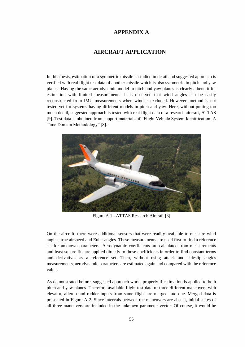
55

APPENDIX A

APPENDICES

A.AIRCRAFT APPLICATION

In this thesis, estimation of a symmetric missile is studied in detail and suggested approach is

verified with real flight test data of another missile which is also symmetric in pitch and yaw

planes. Having the same aerodynamic model in pitch and yaw planes is clearly a benefit for

estimation with limited measurements. It is observed that wind angles can be easily

reconstructed from IMU measurements when wind is excluded. However, method is not

tested yet for systems having different models in pitch and yaw. Here, without putting too

much detail, suggested approach is tested with real flight data of a research aircraft, ATTAS

[9]. Test data is obtained from support materials of “Flight Vehicle System Identification: A

Time Domain Methodology” [8].

Figure A 1 - ATTAS Research Aircraft [3]

On the aircraft, there were additional sensors that were readily available to measure wind

angles, true airspeed and Euler angles. These measurements are used first to find a reference

set for unknown parameters. Aerodynamic coefficients are calculated from measurements

and least square fits are applied directly to those coefficients in order to find constant terms

and derivatives as a reference set. Then, without using attack and sideslip angles

measurements, aerodynamic parameters are estimated again and compared with the reference

values.

As demonstrated before, suggested approach works properly if estimation is applied to both

pitch and yaw planes. Therefore available flight test data of three different maneuvers with

elevator, aileron and rudder inputs from same flight are merged into one. Merged data is

presented in Figure A 2. Since intervals between the maneuvers are absent, initial states of

all three maneuvers are included in the unknown parameter vector. Of course, it would be

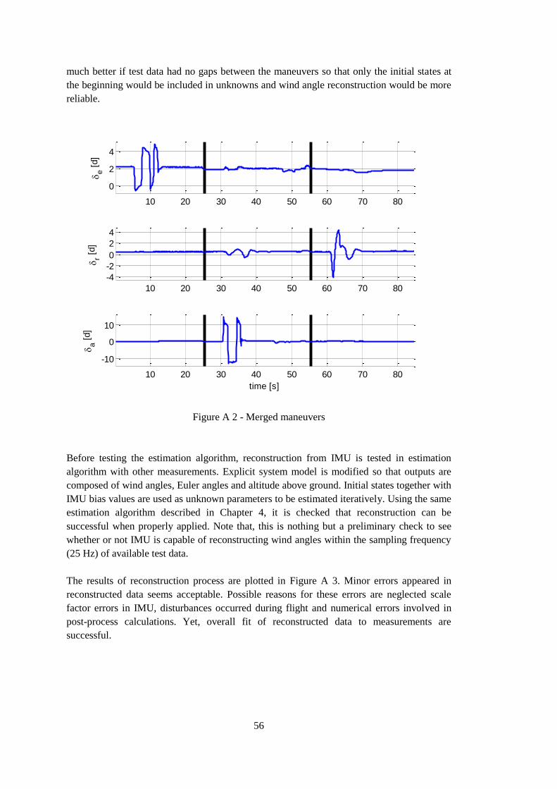
56

much better if test data had no gaps between the maneuvers so that only the initial states at

the beginning would be included in unknowns and wind angle reconstruction would be more

reliable.

Figure A 2 - Merged maneuvers

Before testing the estimation algorithm, reconstruction from IMU is tested in estimation

algorithm with other measurements. Explicit system model is modified so that outputs are

composed of wind angles, Euler angles and altitude above ground. Initial states together with

IMU bias values are used as unknown parameters to be estimated iteratively. Using the same

estimation algorithm described in Chapter 4, it is checked that reconstruction can be

successful when properly applied. Note that, this is nothing but a preliminary check to see

whether or not IMU is capable of reconstructing wind angles within the sampling frequency

(25 Hz) of available test data.

The results of reconstruction process are plotted in Figure A 3. Minor errors appeared in

reconstructed data seems acceptable. Possible reasons for these errors are neglected scale

factor errors in IMU, disturbances occurred during flight and numerical errors involved in

post-process calculations. Yet, overall fit of reconstructed data to measurements are

successful.

10 20 30 40 50 60 70 80

0

2

4

e [

d]

10 20 30 40 50 60 70 80

-4

-2

0

2

4

r [

d]

10 20 30 40 50 60 70 80

-10

0

10

time [s]

a [

d]

57

Figure A 3 - Flight path reconstruction from IMU measurements

0 50 100

02

4

6

8

[

d]

0 50 100

-0.2

0

0.2

0 50 100-4

-2

0

2

4

[

d]

0 50 100-0.3

-0.2

-0.1

0

0.1

0 50 100

-20

0

20

[

d]

0 50 100

-1

0

1

0 50 100

02468

[

d]

0 50 100

-0.2

0

0.2

0 50 100

81012141618

[

d]

0 50 100

-0.2

0

0.2

0 50 100

120

125

130

time [s]

V [

m/s

]

measurements

model outputs with initial values

model outputs with final estimates

errors with final estimates

0 50 100

-0.2

0

0.2

0.4

time [s]

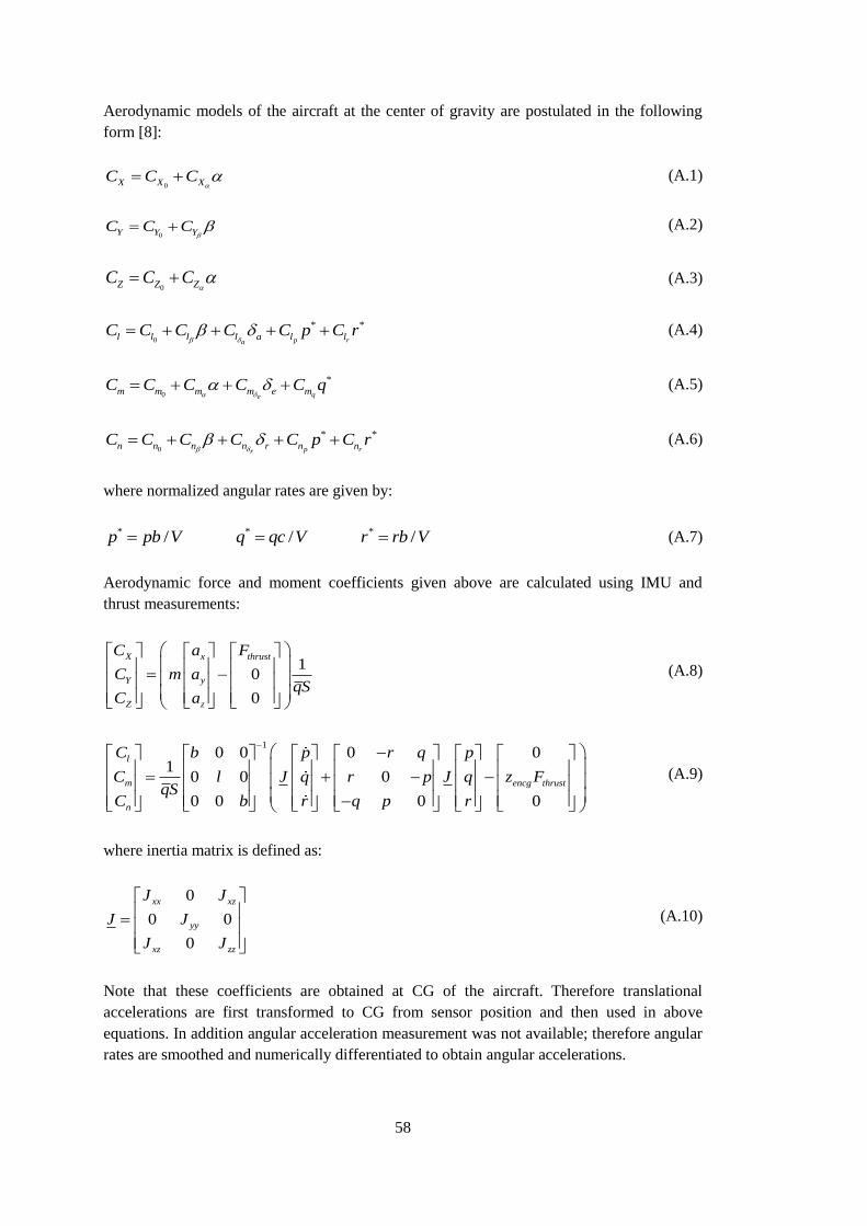
58

Aerodynamic models of the aircraft at the center of gravity are postulated in the following

form [8]:

0X X XC C C (A.1)

0Y Y YC C C (A.2)

0Z Z ZC C C (A.3)

0

* *

p ral l l l ll aC C C C C p rC

(A.4)

0

*

qem m m m e mC C C C C q

(A.5)

0

* *

p rrn n n n nn rC C C C C p rC

(A.6)

where normalized angular rates are given by:

* * */ / /p pb V q qc V r rb V (A.7)

Aerodynamic force and moment coefficients given above are calculated using IMU and

thrust measurements:

10

0

X thrus

Y

z

tx

y

Z

C a

C m a

C a

F

qS

(A.8)

1

0 0 0 01

0 0 0

0 0 0 0

l

m encg thrust

n

C b p r q p

C l J q r p J q z FqS

C b r q p r

(A.9)

where inertia matrix is defined as:

0

0 0

0

xx xz

yy

xz zz

J J

J J

J J

(A.10)

Note that these coefficients are obtained at CG of the aircraft. Therefore translational

accelerations are first transformed to CG from sensor position and then used in above

equations. In addition angular acceleration measurement was not available; therefore angular

rates are smoothed and numerically differentiated to obtain angular accelerations.

59

Using least square estimation, aerodynamic parameters in postulated linear models are

achieved. Then translational accelerations and angular accelerations are evaluated from

estimation results by going backwards in Equations (A.8) and (A.9). Comparison of actual

measurements and model fits are given in Figure A 4.

Aerodynamic parameters are also estimated without wind angles measurements. Maximum

likelihood estimation is applied with explicit system model. However output equations of the

system model are now modified as:

0

0

0

2 10

20

X X thrust

Y Y

Z

x

Z

y

z

FC CaV S

a C Cm m

a C C

(A.11)

0

0

0

2

1 2

2

1 1

0 0

0 0 /2

0 0

0 0

(

0

0

)

( ) /

0

/p ra

qe

p rr

l l l a l l

m m m e m

n n

encg thrus

n r n n

t

C C C C C Vp bS

q J l C C C C q V

r b C C C C C V

r q

p r b

l

p r

J z F J p

b

r

q p

p

J q

r

(A.12)

where total velocity, angle of attack and sideslip parameters appeared in above output

equations are evaluated from states:

2 2 2 1 1 tan ( / ) tan ( / )V u v w w u v u (A.13)

This change is necessary due to the difference between Javelin and ATTAS aerodynamic

models and inertia matrices. Note that translational acceleration and angular acceleration at

X axis are also included to output vector. Since state equations of explicit model do not

involve any aerodynamic parameters, those are remained same.

Comparison of explicit model outputs with final estimates and real measurements are given

in Figure A 5. Correlation coefficients are also checked and it is observed that aerodynamic

parameters are not correlated with any other parameter. Unfortunately estimations of initial

conditions appear as highly correlated which might affect the estimation results. This is most

likely because three different maneuver sets are used as one and two additional initial

condition sets are included to unknown parameters.

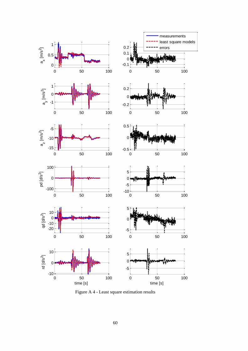
60

Figure A 4 - Least square estimation results

0 50 100

0

0.5

1a

x [

m/s

2]

0 50 100

-0.1

0

0.1

0.2

0 50 100

-1

0

1

ay [

m/s

2]

0 50 100

-0.2

0

0.2

0 50 100

-15

-10

-5

az [

m/s

2]

0 50 100-0.5

0

0.5

0 50 100

-100

0

100

pd [

d/s

2]

0 50 100-10

-5

0

5

0 50 100

-20

-10

0

10

qd [

d/s

2]

0 50 100

-5

0

5

0 50 100-10

0

10

rd [

d/s

2]

time [s]

0 50 100

-5

0

5

time [s]

measurements

least square models

errors

61

Figure A 5 - Maximum likelihood estimation results

0 50 100

0

0.5

1

ax [

m/s

2]

0 50 100

-0.1

0

0.1

0.2

0 50 100

-1

0

1

ay [

m/s

2]

0 50 100

-0.2

0

0.2

0 50 100

-15

-10

-5

az [

m/s

2]

0 50 100

-0.4

-0.2

0

0.2

0 50 100

-100

0

100

pd [

d/s

2]

0 50 100-10

0

10

0 50 100

-20

-10

0

10

qd [

d/s

2]

0 50 100

-4

-2

0

2

4

0 50 100-10

0

10

time [s]

rd [

d/s

2]

measurements

maximum likelihood models

errors

0 50 100

-5

0

5

time [s]

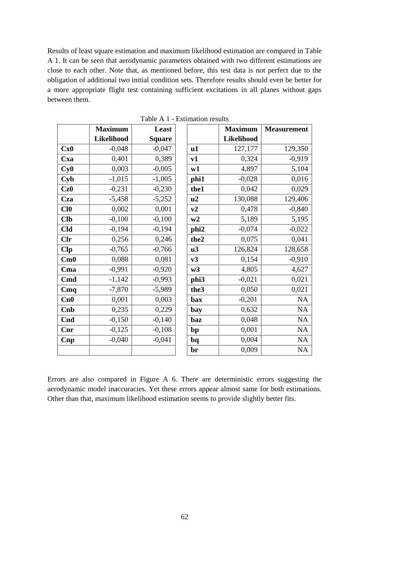
62

Results of least square estimation and maximum likelihood estimation are compared in Table

A 1. It can be seen that aerodynamic parameters obtained with two different estimations are

close to each other. Note that, as mentioned before, this test data is not perfect due to the

obligation of additional two initial condition sets. Therefore results should even be better for

a more appropriate flight test containing sufficient excitations in all planes without gaps

between them.

Table A 1 - Estimation results

Maximum

Likelihood

Least

Square

Maximum

Likelihood

Measurement

Cx0 -0,048 -0,047 u1 127,177 129,350

Cxa 0,401 0,389 v1 0,324 -0,919

Cy0 0,003 -0,005 w1 4,897 5,104

Cyb -1,015 -1,005 phi1 -0,028 0,016

Cz0 -0,231 -0,230 the1 0,042 0,029

Cza -5,458 -5,252 u2 130,088 129,406

Cl0 0,002 0,001 v2 0,478 -0,840

Clb -0,100 -0,100 w2 5,189 5,195

Cld -0,194 -0,194 phi2 -0,074 -0,022

Clr 0,256 0,246 the2 0,075 0,041

Clp -0,765 -0,766 u3 126,824 128,658

Cm0 0,088 0,081 v3 0,154 -0,910

Cma -0,991 -0,920 w3 4,805 4,627

Cmd -1,142 -0,993 phi3 -0,021 0,021

Cmq -7,870 -5,989 the3 0,050 0,021

Cn0 0,001 0,003 bax -0,201 NA

Cnb 0,235 0,229 bay 0,632 NA

Cnd -0,150 -0,140 baz 0,048 NA

Cnr -0,125 -0,108 bp 0,001 NA

Cnp -0,040 -0,041 bq 0,004 NA

br 0,009 NA

Errors are also compared in Figure A 6. There are deterministic errors suggesting the

aerodynamic model inaccuracies. Yet these errors appear almost same for both estimations.

Other than that, maximum likelihood estimation seems to provide slightly better fits.

63

Figure A 6 - Error comparison of estimations

To sum up, maximum likelihood estimation without wind angle measurements can also be

applied to aircrafts under appropriate circumstances. Limitations given for a symmetric

missile still holds here. Test data to be used in estimation must contain sufficient information

for all planes so that wind angles reconstruction can be done without any correlations.

Moreover wind must not be existed during the excitations of system. Otherwise

reconstructed wind angles will not be exact and resulting parameter estimates will be biased.

Even if above conditions cannot be met exactly, maximum likelihood estimation with

explicit system model suggested in this thesis may be used to obtain rough models for

aircrafts.

1

0 50 100

-0.1

0

0.1

0.2

ax [

m/s

2]

0 50 100

-0.2

0

0.2

ay [

m/s

2]

0 50 100

-0.5

0

0.5

az [

m/s

2]

0 50 100-10

0

10

pd [

d/s

2]

0 50 100

-5

0

5

qd [

d/s

2]

time [s]

0 50 100

-5

0

5

rd [

d/s

2]

time [s]

least square errors

maximum likelihood errors