aero-acoustic assessment of installed...
TRANSCRIPT
INCAS BULLETIN, Volume 7, Issue 2/ 2015, pp. 53 – 62 ISSN 2066 – 8201
Aero-Acoustic assessment of installed propellers
Marius Gabriel COJOCARU*,1
, Mihai Leonida NICULESCU1,
Mihai Victor PRICOP1
*Corresponding author
*,1
INCAS – National Institute for Aerospace Research “Elie Carafoli”
B-dul Iuliu Maniu 220, Bucharest 061126, Romania
[email protected]*, [email protected], [email protected]
DOI: 10.13111/2066-8201.2015.7.2.5
3rd
International Workshop on Numerical Modelling in Aerospace Sciences, NMAS 2015,
06-07 May 2015, Bucharest, Romania, (held at INCAS, B-dul Iuliu Maniu 220, sector 6)
Section 2 – Flight dynamics simulation
Abstract: The volume of general aviation transport is increasing and consequently this gives rise to
the need for reducing noise levels while improving or at least maintaining the same level of
aerodynamic performance. This can be achieved through the use of modern propellers and engines. In
this paper we present a methodology to study and predict the installed propeller noise at the same
time with the aerodynamic characterization, through the use of unsteady CFD and Acoustic-Analogies
analysis. The analysis shows the influence of different acoustic sources generated by the installed
propeller on the far field noise by monitoring the monopoles and dipoles with and without taking into
account the quadrupoles. In this way we can observe the influence of the distance from the propeller
to the engine intake on the overall sound. Time averaged aerodynamic performances are presented
along with instantaneous results.
Key Words: Aeroacoustic, CFD, Propeller, Ffowcs-Williams Hawkings, Direct Sound Computation.
1. INTRODUCTION
The present paper presents a CFD method for computing the aerodynamic performances of a
general aviation turboprop powered aircraft and its propeller. Then two aeroacoustic
methods are presented for computing the noise levels, at far and near points, and the results
are compared against each other. One method is based on the Direct Sound Computation
within the CFD simulation while the other is based on the Ffowcs-Williams Hawkings
acoustic analogy. Finally, the contribution to noise levels is analyzed for each noise source
and the installation effects are summarized.
2. SOLVER SETTINGS AND MODELLING SIMPLIFICATIONS
Ansys - Fluent is a CFD software that has a very broad range of applications. The code uses
the finite volume approach to discretize the Navier-Stokes equations (and their
approximations Reynolds-Averaged Navier-Stokes, Large Eddy Simulation, etc.) and a wide
array of related equations such as energy conservation, passive scalar transport equations,
heat transfer, chemical reactions, noise propagation, etc. to solve the fluid flow and fluid
flow related problems. This flexibility allows us to use Fluent to solve the compressible fluid
flow around a propeller with nacelle and wing for aeroacoustic and aerodynamic purposes.
Marius Gabriel COJOCARU, Mihai Leonida NICULESCU, Mihai Victor PRICOP 54
INCAS BULLETIN, Volume 7, Issue 2/ 2015
The assumptions made in the current computation are:
• The medium is considered to be a continuum.
• The flow is turbulent over the full domain.
• The equation of state is for an ideal gas.
• The flow is compressible.
• The equations are cast in the conservative form, and the solver is “density based”,
Roe method for flux discretization.
• The solution sought corresponds to an unsteady state.
• The influence of the fuselage on the flow field and noise scattering is minimal;
therefore at the wing root a symmetry plane is introduced for the sake of simplicity.
• The chemical composition of the jet is identical to the air.
• Monopoles, dipoles and quadrupoles are accounted as acoustic sources.
• The airplane is in “climb after take-off” condition.
• The solver has a time-step in seconds chosen such that it that corresponds to 2°/time-
step in propeller rotations.
Since we assume the flow to be governed by a compressible ideal gas at a fully turbulent
regime in unsteady conditions we can use the URANS equations. The RANS approach is
based on the k-ω STT turbulence model that uses the Boussinesq hypothesis.
This model was proposed by Menter and combines the advantages of traditional Low-
Reynolds k-ω models near the wall with the classical k-ε models far from the walls, the two
models are combined through blending functions.
This model has proved to be useful in computing flows in rotating domains and
accurately predicting boundary layer separation and aerodynamic forces/moments for largely
separated steady flows.
The equations are solved in the implicit approach and solution acceleration is made
using the Algebraic Multi-Grid method.
Time integration is performed in the dual-time approach proposed by Jameson, and
ensures the second order time accuracy. The existence of the Ffowcs – Williams Hawkings
(FWH) model for predicting the far-field noise into Ansys Fluent allows us to perform the
acoustic analysis.
Also the Ansys Fluent is able to perform Direct Sound Computation by monitoring the
unsteady pressure fluctuations at specific locations; afterwards this data is transformed into
Sound Pressure Levels (SPL) by using an adequate FFT (Fast Fourier Transform) solver.
The specific workflow for aeroacoustic computations is described hereafter:
1. The steady flow solution is computed in the specified regime, with the Multiple
Reference Frame (MRF) method.
2. The unsteady solver is initialized with the steady flow solution and run for a number
of at least 4 revolutions. The number of 4 full revolutions is obtained from
experience in similar cases and is sufficient for the solver to “wash” away any
unphysical solutions that arose from the initialization process. The MRF is changed
into a sliding mesh method to model the propeller actual rotation.
3. Afterwards the FWH acoustic solver is switched on and monitoring for acoustic
sources begins.
4. The unsteady solution is computed for another 2-3 full revolutions. The actual
number of revolutions is calculated so that the acoustic perturbations have plenty of
time to reach the locations where the sound is going to be measured.
5. The FHW acoustic analogy is performed for all the “microphone” locations.
55 Aero-Acoustic assessment of installed propellers
INCAS BULLETIN, Volume 7, Issue 2/ 2015
Alternatively, for a Direct Sound Computation we set up monitoring points in the zone
near the propeller and monitor there the unsteady pressure fluctuations. The pressure
fluctuations are transformed in SPL and then corrected as if they were located on the surface
of a sphere at 8 times the radius of the previous one.
The correction takes place in the following manner, for each doubling of the distance the
SPL drops by 6dB.
The proof for this is very simple: let us assume that we have sound propagating as a
spherical wave and we take a look at two instants, one at radius r1 and one at r2. The noise
that generates this wave is characterized by the power P and at radius r1 by the acoustic
intensity I1 = P/4πr12 and at r2 by I2 = P/4πr2
2.
By dividing them we get that I2/I1 ~ r12/r2
2, and knowing that I ~ p
2, we get that p ~ 1/r,
where p stands for pressure.
Now by using the formula SPL = 20log10(p/p0) (where p0 is a reference pressure for
sound traveling in air at normal conditions and is equal to p0 = 20μPa) we get that for the
difference in: SPL2 – SPL1 = 20log10(p2/p1) = 20log(r1/r2 = 1/2) = 6.02dB. Therefore for
correcting for the sound on a sphere located at 8 (=23) times the radius of the previous one
we simply get the SPL and subtract 18 (=3·6).
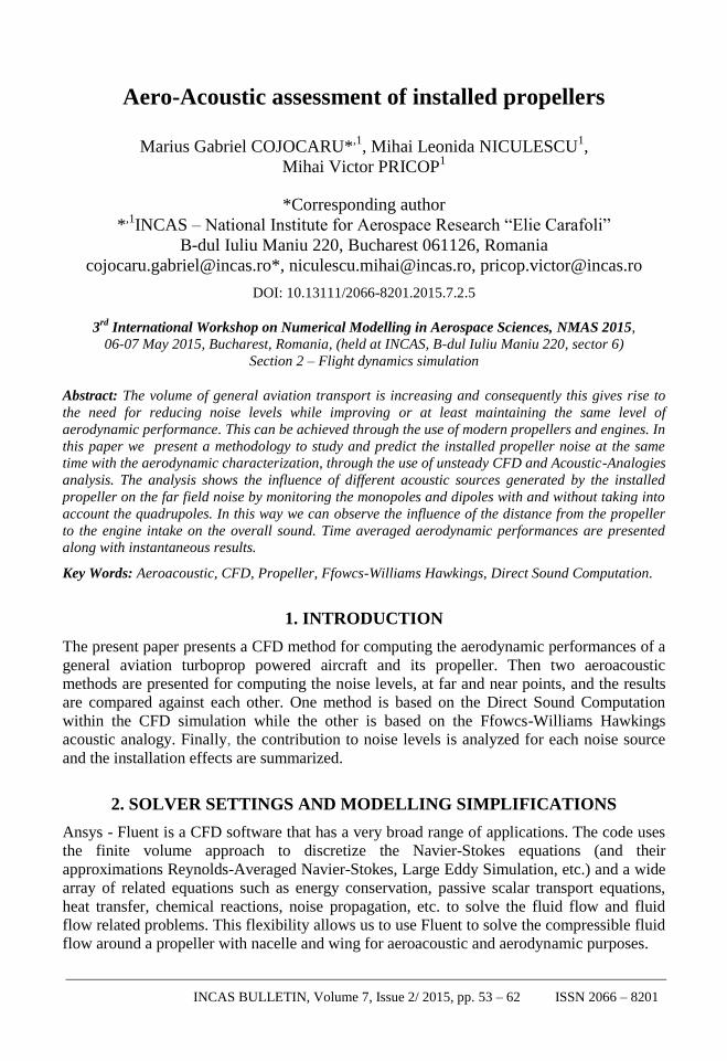
3. GEOMETRY AND MESHING
Geometry and modeling assumptions and simplifications are given on short below:
The flow inside the nacelle is ignored.
All the nacelle’s ventilation inlets/outlets are closed.
The wing flap is ignored since there is no need to model the noise generated by it.
The domain is split in a rotating part and a fixed one with respect to the reference
frame.
An exhaust jet domain is constructed to refine the mesh in that region.
Fig. 1. – Geometry and computational domain
The mesh is constructed in Numeca’s Hexpress and is based on a hexahedral volume-to-
surface approach. The total number of elements is 18M cells for the fixed domain, 20M cells

Marius Gabriel COJOCARU, Mihai Leonida NICULESCU, Mihai Victor PRICOP 56
INCAS BULLETIN, Volume 7, Issue 2/ 2015
for the rotor and 2M cells for the jet region.
The mesh was constructed as having a target of 25 Points-Per-Wavelength (PPW) in the
rotor area near the blade and 23.5 PPW in the wake refinement region. The PPW cell size is
based on the propeller Blade Passing Frequency (BPF) multipled by 5 that is estimated to be
at 146.67·5 Hz and this leads to a propeller wavelength of λPropeler = 0.46m.
The factor of 5 comes from the fact that we are interested in monitoring at least 4 BPF
accurately; this is why we chose to have a larger number of BPFs as reference frequency.
The table with point coordinates where the “microphones” are placed is given.
For the radius of 1.2m (near field) the sound is computed directly from pressure
fluctuations and for the radius of 9.6m, the sound is computed from FWH or by simply
correcting the near field computed sound.
Fig. 2. – Mesh for the aerodynamic computations. Median plane
Fig. 3. – Locations of points in the near field (left) and far field (right)

57 Aero-Acoustic assessment of installed propellers
INCAS BULLETIN, Volume 7, Issue 2/ 2015
Fig. 4. – Locations of points in the near field and far field, with an increment of 15°
4. NUMERICAL RESULTS
The aerodynamic and aeroacoustic sources and noise have been computed using Ansys –
Fluent. The flow condition chosen represents the “climb after take-off” condition and it
translates into:
• Propeller Rotational speed: 2200 RPM
• Altitude: 0m
• Temperature: ISA + 0°C
• Speed: 130km/h TAS
• Aircraft Angle of Attack: 7°
• Engine Inlet Mass-flow Rate: 2.4 kg/s.
The flow field is computed first for the steady state with a fixed mesh, the propeller
rotation is modelled by rotating the reference frame of the domain that contains it. This
steady state is taken as the initial condition for the unsteady solver.
The unsteady solver this time uses the sliding mesh technique to rotate the propeller at
the imposed rotational speed. To exchange information in between domains special
interfaces are modeled.
Flow solution after 1.5 revolutions Flow solution after 3.5 revolutions
Fig. 5. – Vorticity field in the median plane. Pressure contours on the surface
Marius Gabriel COJOCARU, Mihai Leonida NICULESCU, Mihai Victor PRICOP 58
INCAS BULLETIN, Volume 7, Issue 2/ 2015
The flow field after 3-4 revolutions is free from the unphysical solution, that is present
at t =1.5 revolutions, due to the initialization and sudden start of the rotation.
The wake vortices are dissipated far after the propeller due to the increase in grid size.
Therefore after 4 complete revolutions the FWH acoustic solver is set to monitor for acoustic
sources on solid surfaces that form the blades + spinner and the nacelle.
Supplementary to this another ten sources (points 1 to 10 in the table above) in the near
field are set up to monitor the unsteady pressure fluctuation to allow us to compute the sound
in a direct manner.
This is run for another 2-3 revolutions to build a database for the acoustics. Points 1-10
in the near field correspond radially to points 11-23 respectively in the far field.
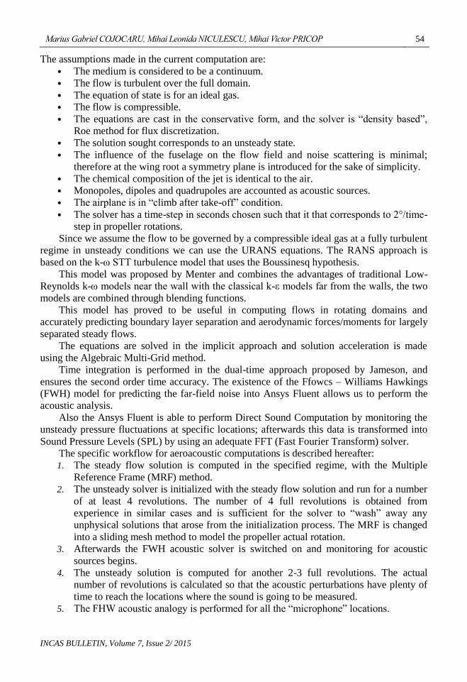
The FWH solver by monitoring only solid surfaces as sources takes into account only
monopoles and dipoles. The results obtained with the DSC and the FWH analogy are
presented hereafter.
Fig. 6. - Validation of DSC with FWH on near points
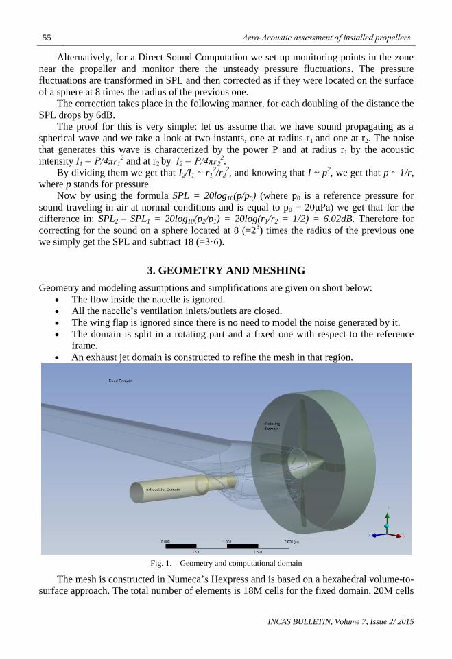
Fig. 7. - Different acoustic sources noise levels at far points and their respective contributions to OASPL
FWH method

59 Aero-Acoustic assessment of installed propellers
INCAS BULLETIN, Volume 7, Issue 2/ 2015
Fig. 8. - Frequency-by-frequency analysis on the far points. DSC method
Fig. 9. – Sound Pressure Levels of the near points. DSC and FWH method
Fig. 10. - Sound Pressure Levels of the near points. DSC and FWH method

Marius Gabriel COJOCARU, Mihai Leonida NICULESCU, Mihai Victor PRICOP 60
INCAS BULLETIN, Volume 7, Issue 2/ 2015
Fig. 11. - Sound Pressure Levels of the near points. DSC and FWH method
Fig. 12. - Sound Pressure Levels of the far points. FWH method
Fig. 13. - Sound Pressure Levels of the far points. FWH method
61 Aero-Acoustic assessment of installed propellers
INCAS BULLETIN, Volume 7, Issue 2/ 2015
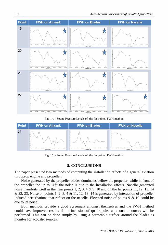
Fig. 14. - Sound Pressure Levels of the far points. FWH method
Fig. 15. - Sound Pressure Levels of the far points. FWH method
5. CONCLUSIONS
The paper presented two methods of computing the installation effects of a general aviation
turboprop engine and propeller.
Noise generated by the propeller blades dominates bellow the propeller, while in front of
the propeller the up to -45° the noise is due to the installation effects. Nacelle generated
noise manifests itself in the near points 1, 2, 3, 4 & 9, 10 and on the far points 11, 12, 13, 14
& 22, 23. Noise on points 1, 2, 3, 4 & 11, 12, 13, 14 is generated by interaction of propeller
induced perturbations that reflect on the nacelle. Elevated noise of points 9 & 10 could be
due to jet noise.
Both methods provide a good agreement amongst themselves and the FWH method
could have improved results if the inclusion of quadrupoles as acoustic sources will be
performed. This can be done simply by using a permeable surface around the blades as
monitor for acoustic sources.

Marius Gabriel COJOCARU, Mihai Leonida NICULESCU, Mihai Victor PRICOP 62
INCAS BULLETIN, Volume 7, Issue 2/ 2015
REFERENCES
[1] O. Labbe, C. Peyret, G. Rahier. M. Huet, A CFD/CAA coupling method applied to jet noise prediction,
Computers and fluids, vol. 86, pp 1-13, 2013.
[2] A. Filippone, Aircraft noise prediction, Progress in Aerospace Sciences, vol. 86, pp. 27-63, 2014.
[3] A. Giaque, B. Ortun, B. Rodriguez, B. Caruelle, Numerical error analysis with application to transonic
propeller aeroacoustics, Computers and Fluids, vol. 69, pp. 20-34, 2012.
[4] G. Bennett, J. Kennedy, C. Meskell, M. Carley, P. Jordan, H. Rice, Aeroacoustic research in Europe: The
CEAS-ASC report 2013 highlights, Journal of Sound and Vibration, vol. 340, pp. 39-60, 2015.
[5] J. Yin, A. Stuermer, M. Aversano, Coupled uRANS and FW-H Analysis of Installed Pusher Propeller Aircraft
Configurations, 15-th AIAA Aeroacoustics Conference, 2009.
[6] * * * Ansys Fluent Theory Guide, release 15, 2013.
[7] * * * Ansys Fluent User’s Guide, release 15, 2013.