aerial electromagnetic sounding of the lithosphere …dstillman/pdf/grimm_icarus_2011pip.pdf ·...

Icarus xxx (2011) xxx–xxx

Contents lists available at SciVerse ScienceDirect

Icarus

journal homepage: www.elsevier .com/locate / icarus

Aerial electromagnetic sounding of the lithosphere of Venus

Robert E. Grimm a,⇑, Amy C. Barr a, Keith P. Harrison a, David E. Stillman a, Kerry L. Neal b,Michael A. Vincent b, Gregory T. Delory c

a Dept. of Space Studies, Southwest Research Institute, 1050 Walnut St. #300, Boulder, CO 80302, United Statesb Dept. of Space Operations, Southwest Research Institute, 1050 Walnut St. #300, Boulder, CO 80302, United Statesc Space Sciences Laboratory, University of California, 7 Gauss Way, Berkeley, CA 94720, United States

a r t i c l e i n f o a b s t r a c t

Article history:Available online xxxx

Keywords:Venus, InteriorLightningGeophysicsThermal historiesIonospheres

0019-1035/$ - see front matter � 2011 Elsevier Inc. Adoi:10.1016/j.icarus.2011.07.021

⇑ Corresponding author. Fax: +1 303 546 9687.E-mail address: [email protected] (R.E. Gri

Please cite this article in press as: Grimm, Rj.icarus.2011.07.021

Electromagnetic (EM) investigation depths are larger on Venus than Earth due to the dearth of water inrocks, in spite of higher temperatures. Whistlers detected by Venus Express proved that lightning is pres-ent, so the Schumann resonances �10–40 Hz may provide a global source of electromagnetic energy thatpenetrates �10–100 km. Electrical conductivity will be sensitive at these depths to temperature structureand hence thermal lithospheric thickness. Using 1D analytic and 2D numerical models, we demonstratethat the Schumann resonances—transverse EM waves in the ground-ionosphere waveguide—remain sen-sitive at all altitudes to the properties of the boundaries. This is in marked contrast to other EM methodsin which sensitivity to the ground falls off sharply with altitude. We develop a 1D analytical model foraerial EM sounding that treats the electrical properties of the subsurface (thermal gradient, water con-tent, and presence of conductive crust) and ionosphere, and the effects of both random errors and biasesthat can influence the measurements. We initially consider specified 1D lithospheric thicknesses 100–500 km, but we turn to 2D convection models with Newtonian temperature-dependent viscosity to pro-vide representative vertical and lateral temperature variations. We invert for the conductivity-depthstructure and then temperature gradient. For a dry Venus, we find that the error on temperature gradientobtained from any single local measurement is �100%—perhaps enough to distinguish ‘‘thick’’ vs. ‘‘thin’’lithospheres. When averaging over thousands of kilometers, however, the standard deviation of therecovered thermal gradient is within the natural variability of the convection models, <25%. A ‘‘wet’’ inte-rior (hundreds of ppm H2O) limits EM sounding depths using the Schumann resonances to <20 km, anderrors are too large to estimate lithospheric properties. A 30-km conductive crust has little influence onthe dry-interior models because the Schumann penetration depths are significantly larger. We concludethat EM sounding of the interior of Venus is feasible from a 55-km high balloon. Lithospheric thicknesscan be measured if the upper-mantle water content is low. If H2O at hundreds of ppm is present, the dee-per, temperature-sensitive structure is screened, but the ‘‘wet’’ nature of the upper mantle, as well asstructure of the upper crust, is revealed.

� 2011 Elsevier Inc. All rights reserved.

1. Introduction

The geodynamic style of a solid planet or satellite is controlledby the thickness of its lithosphere, or strong, comparatively cold,outer shell. The coherent part is formally the mechanical litho-sphere, whereas the thermal lithosphere is the (generally thicker)conductive boundary layer to internal solid-state convection. Wetreat the thermal lithosphere in this paper, and denote its maxi-mum and mean thicknesses as L and L, respectively.

Earth’s lithosphere has been globally investigated throughearthquake seismology, with additional contributions from othergeophysical methods. L ¼ 100 km for oceanic lithosphere and

ll rights reserved.

mm).

.E., et al. Aerial electromagne

L ¼ 200 km for continental lithosphere (Schubert et al., 2001). So-lid-state convection in the Earth has a freely moving lithosphere100 km thick—plate tectonics—because temperature-dependentviscosity contrasts are modest (Solomatov, 1995), probably moder-ated by the presence of water.

The unknown mean thickness and variability of the lithosphereof Venus are major obstacles to characterizing its geodynamicstyle. The best constraints at present come from the correlation be-tween gravity and topography, which indicates apparent depths ofAiry isostatic compensation of 150–350 km for spherical harmonicdegrees 3–10 (Sjogren et al., 1997). Local correlations, expressedalternatively as geoid-to-topography ratio (GTR), indicate Prattcompensation depths of 140–400 km for the volcanic rises, withan average value around 260 km (Moore and Schubert, 1997).The Pratt compensation depth is equivalent to L.

tic sounding of the lithosphere of Venus. Icarus (2011), doi:10.1016/

http://dx.doi.org/10.1016/j.icarus.2011.07.021

mailto:[email protected]


http://www.sciencedirect.com/science/journal/00191035

http://www.elsevier.com/locate/icarus



1 2 3 4 5 6

0

100

200

300

400

Log10 ρ, Ω−m

Dep

th, k

m

−6 −5 −4 −3 −2 −1 0 1 21

1.5

2

2.5

3

Log10 Freq., Hz

Log 10

Exp

lor.

Dep

th, k

m

a

b

Fig. 1. (a) Comparison of electrical resistivity on Earth and Venus. Blue: Earthstructure (dashed: smoothed model of Egbert and Booker (1992); solid: layeredmodel of Lizarralde et al. (1995)). Remaining curves are Venus: solid, dry; dashed,wet (�200–600 ppm H2O). Black, green, red: lithospheric thicknesses of 400, 200,and 100 km, respectively. (b) Comparison of electromagnetic (EM) investigationdepths. Increase in resistivity due to dry rocks on Venus more than offsets decreasein resistivity due to temperature, so that effective penetration depths are muchlarger on Venus. This enables sounding of the upper mantle by lightning-causedSchumann resonances at �10–40 Hz. (For interpretation of the references to colorin this figure legend, the reader is referred to the web version of this article.)

2 R.E. Grimm et al. / Icarus xxx (2011) xxx–xxx

A lithospheric thickness significantly greater than Earth’s is notconsistent with heat flow scaled from Earth or from chondriticmeteorites. Purely conductive equilibrium with terrestrial heatsources would lead to L ¼ 40—45 km, too thin to support large-scale topography (Solomon and Head, 1982; Turcotte, 1995).Parameterized-convection models using chondritic heat sourcesand a free upper boundary (or small viscosity contrast) produceabout three-quarters of the current terrestrial flux after 4 billionyears (Phillips and Malin, 1983; Solomatov and Moresi, 1996) so,scaling from oceanic lithosphere, L < 150 km for a ‘‘plate-tectonic’’Venus. (Also, Kaula and Phillips (1981) derived L ¼ 94 km directlyfrom thermal-boundary layer theory using terrestrial heat flux.)Yet there is no evidence for contemporary lithospheric recyclingin the geological record of Venus (Solomon et al., 1992). If indeedL ¼ 200—300 km and Venus has a chondritic or terrestrial comple-ment of radionuclides, then ‘‘Venus cannot presently be in anapproximate thermal steady state’’ (Schubert et al., 1997).

Numerical models of mantle convection suggest that stronglytemperature-dependent viscosity leads to such large contrasts thatthe lithosphere becomes stationary (Solomatov and Moresi, 1996).Such ‘‘stagnant-lid’’ convection could be a consequence of a dearthof water. Imposition of a stagnant lid 0.6–2 byr ago in parameter-ized-convection models reduces current heat flow to as low as30% of the value just prior to stagnation (Solomatov and Moresi,1996; Phillips et al., 1997). The stagnant lid cools while the deeperinterior heats up—an evolution away from equilibrium that hasbeen postulated to trigger episodic lithospheric foundering andglobal resurfacing (Turcotte, 1993).

The harsh surface conditions of Venus and large resourcerequirements pose serious challenges to a network of long-livedgeophysical stations that might further probe the lithosphere inaccustomed ways. Seismic coupling to the dense atmosphere ofVenus could be detectable as ionospheric perturbations, thus en-abling seismology from orbit (Lognonné et al., 2005). A satelliteconstellation is necessary, however, for optimum implementation.Another way to exploit the dense atmosphere for subsurface inves-tigation is to perform electromagnetic sounding from a balloon inthe relatively benign environment near 55-km altitude. Balloonsare a component of the Venus Flagship concept definition (Bullocket al., 2009) and have been considered by others for Discovery(NASA) or Cosmic-Vision (ESA) class missions (Wilson et al.,2011). The pioneering VEGA balloons lasted a few days (Sagdeevet al., 1986), but balloon longevity can potentially be measuredin circumnavigations.

We present a series of numerical and analytical models to dem-onstrate the feasibility of aerial electromagnetic sounding onVenus, specifically to determine lithospheric thickness—the pivotalgeodynamic parameter. The relevant natural sources are discussed,and how the unique properties of the ground-ionosphere wave-guide enable high-altitude EM sounding. Measurement errors areincorporated and a new high-performance sensor configuration isproposed. Subsurface temperature profiles are specified or aretaken from numerical models of mantle convection. Tempera-ture-dependent electrical conductivity of the ground is calculatedfrom laboratory measurements of either dry or ‘‘wet’’ olivine. Theionospheric conductivity is also considered. Particular attentionis given to the effects of ionospheric variability on the inferenceof ground conductivity, as boundary coupling in effect generatesa joint ionosphere-subsurface inverse problem.

2. Electromagnetic sounding

2.1. Earth–Venus comparison

Electromagnetic (EM) sounding encompasses a wide variety ofmethods used to sense subsurface structure from less than a few

Please cite this article in press as: Grimm, R.E., et al. Aerial electromagnej.icarus.2011.07.021

meters to a thousand kilometers or more (see Telford et al.,1990; Simpson and Bahr, 2005; Grimm, 2009, for reviews). Below1 Hz, abundant natural energy exists on Earth from magneto-spheric pulsations and from the interaction of the magnetospherewith diurnal heating of the ionosphere. Above 1 Hz, the ground-ionosphere waveguide allows lightning energy to be recordedglobally as the 8–34 Hz Schumann resonances and regionally ashigher frequency impulses.

The fundamental parameter controlling EM exploration is theskin depth d (km) = 0.5

pqa/f (e.g., Telford et al., 1990), where qa

is the apparent resistivity (X m) of the ground and f is the fre-quency (Hz). The apparent resistivity is the resistivity of a half-space that is equivalent to the (depth-dependent) ground undertest. We drop the subscript for convenience and allow all resistiv-ities to be apparent values unless otherwise noted, such as for spe-cific material properties. The exploration depth

D ðkmÞ ¼ 0:36p

q=f ð1Þ

is a better representation of depths at which true resistivity can berecovered (e.g., McNeill, 1990) and figures directly in the asymp-totic inversion used here (Section 3.6).

We compare subsurface electrical resistivity on Earth andVenus and implications for EM sounding in Fig. 1. Representativeresistivity-depth profiles for Earth follow Egbert and Booker(1992) and Lizarralde et al. (1995). The Venus profiles were con-structed by specifying temperature vs. depth and then laboratoryconductivity-temperature measurements were used to form resis-tivity vs. depth (Section 3.2). The lower resistivity of the terrestriallithosphere and upper asthenosphere, even compared to the Venus




R.E. Grimm et al. / Icarus xxx (2011) xxx–xxx 3

‘‘wet’’ (hundreds of ppm H2O) profiles, is likely due to aqueous flu-ids and/or graphite films (e.g., Yoshino et al., 2009).

We calculated the apparent resistivity of a layered halfspaceusing a classical recursion procedure (Wait, 1970; see applicationin Grimm, 2002). This approach includes both diffusion and prop-agation; the latter was disabled here for clarity. The frequency-dependent exploration depth then follows readily. (The reader willnow note that we switch between conductivity and resistivity inthis paper. They are of course reciprocal quantities: geophysicistsoften prefer resistivity due to its dimensional relation to imped-ance, whereas physicists use conductivity as the proportionalityconstant between electric field and current density. However, onlyresistivity is treated as an apparent or halfspace-equivalent value).

Typical Earth resistivities of 1–100 X m can require frequencies<10�5 Hz (i.e., periods of days) to penetrate hundreds of kilometers(Fig. 1). Such measurements have been useful in characterizing thelithosphere, asthenosphere, and mantle transition zone, but can bevery challenging to make. Even exploration to tens of kilometersdepth calls for frequencies in the millihertz range, which still needlong, stationary, ground measurements. For Venus, however, thepresumed dearth of water makes resistivities much higher andhence allows for deeper exploration (Fig. 1). At 10 Hz, for example,D can be up to 130 km. Venus-analog materials that approach1 MX m imply exploration depths 100 times greater than Earthat the same frequency. Alternatively, the same depth can besounded at a frequency 104 times higher than on Earth.

This is the first enabling factor for EM exploration of the subsur-face of Venus: the crust and upper mantle can be probed >1 Hz in-stead of �1 Hz as for Earth. This has several benefits. It allowsspecific sources (Section 2.2) and propagation properties (Sec-tion 2.3) to be exploited. All EM measurements will enjoy highersignal-to-noise ratio (SNR) due to integration of more cycles in aspecified time. Most importantly, electric fields can be measuredcapacitively, because impedance decreases in direct proportion tofrequency.

2.2. EM sources: lightning detection on Venus and the Schumannresonances

Venus lacks the geomagnetic-band (<1 Hz) magnetospheric-pulsation and ionospheric-dynamo signals that are all-importantto deep EM exploration on Earth, but this does not matter becauseof the frequency shift expected for the relatively dry interior. Thespheric band (>1 Hz) is so named on Earth because it is dominatedby ‘‘radio atmospherics,’’ a variety of signals due to lightning dis-charges. Impulsive signals at several kHz to MHz are useful tounderstand the lightning source, but have unfavorable geometricalproperties for high-altitude EM sounding (Section 2.3). These sig-nals are probably propagative in the venusian subsurface (loss tan-gent �1) and penetrate just the top few kilometers.

The nearly continuous lightning discharge rate on Earth(�100 s�1) globally fills the ground-ionosphere waveguide and setsup longitudinal normal modes, the Schumann resonances (seeNickolaenko and Hayakawa, 2002, for a review). Each mode con-tains an integral multiple of wavelengths around the planet: anideal spherical cavity (vacuum between perfect boundary conduc-tors) has eigenfrequencies

fm ¼c

2pa

ffiffiffiffiffiffiffiffiffiffiffiffiffiffiffiffiffiffiffiffiffimðmþ 1Þ

pð2Þ

where c is the speed of light in vacuum, m = 1, 2, 3, . . ., and a is theplanetary radius. Earth’s readily measured Schumanns lie at 8, 14,20, 26, and 32 Hz, which are lower than predicted for the ideal cav-ity due to conduction losses. The quality factor Q measures the abil-ity to sustain propagation in the face of conduction losses into theground or ionosphere. Nickolaenko and Hayakawa (2002) show that


Q is the ratio of the waveguide thickness to the skin depth in theboundary conductor(s). For Earth, the skin depth in the ground (orocean) is negligible and Q = 4–8 over the first four frequencies dueto ionospheric losses.

Several groups have studied the likely properties of Schumannresonances on Venus (Nickolaenko and Rabinowicz, 1982; Pechonyand Price, 2004; Simões et al., 2008). Ideal-waveguide frequenciesdiffer only by the ratio of planetary radii, i.e., the fundamentaleigenfrequency would lie at 11 Hz. Ionospheric conductivity low-ers the fundamental to 9 Hz with estimates of Q from 5 to 10 forthis mode. Simões et al. (2008) also modeled a lossy lower bound-ary, i.e., finite ground conductivity. They adopted a model temper-ature profile from Arkani-Hamed (1994) but simply choseconductivity measurements for ‘‘silicon oxide’’ and for felsic rocks,neither of which is appropriate for a nearly anhydrous, mafic,venusian crust and upper mantle. Simões and co-workers consid-ered an alternative model with conductivity reduced by a factorof 100, but these high- and low-conductivity profiles are still abouta factor of 100 more conductive than our models (Section 3.2)using ‘‘wet’’ and dry olivine, respectively. The fundamental eigen-frequency in their joint ionosphere-ground model falls to 8 Hzand Q = 4. The eigenfrequencies and quality factors could both belower if the higher resistivities used here were adopted.

Evidence for lightning on Venus—the necessary source for theSchumann resonances—has been debated for nearly three decades(see Grebowsky et al., 1997, for a review). We view the recent mea-surements from the Venus Express (VEX) vector magnetometer asdefinitive evidence for lightning. Russell et al. (2007) reportedbursts of field-aligned, circularly-polarized energy near the space-craft periapsis. This is a diagnostic signature of a whistler wavethat is vertically refracted through the ionosphere as it traversesfrom below. Whistlers are uniquely associated with lightning be-cause the dispersion arises from an impulsive source (the actualdispersion cannot be observed by VEX due to bandwidth limita-tion). Russell et al. (2008) refined the estimate of flash rate to18 s�1, about 20% of Earth’s. The amplitudes are, however, un-known. The Schumann excitation is proportional to the currentmoment, or current times (return) stroke length (see Nickolaenkoand Hayakawa, 2002). R strokes per second contribute an ampli-tude multiplier between

pR and R, depending on whether the sig-

nals add incoherently or coherently, respectively. Thus theestimated difference in flash rate will multiply the Venus Schu-mann amplitudes by 0.2–0.4. This could be offset by larger peakcurrents or longer stroke lengths on Venus. The cloud-to-grounddistance, for example, is an order of magnitude larger on Venus.Without any other information, we will assume an Earth-like300 lV/m for the vertical electric field and 1 pT for the horizontalmagnetic field. It is also worth noting that at lower flash rates theTEM excitation may appear as discrete pulses, akin to terrestrialQ-bursts, instead of a continuous harmonic signal.

This is the second enabling factor for EM exploration of the sub-surface of Venus: abundant natural energy, in the form of light-ning-caused Schumann resonances, is very likely to exist in thedesired exploration bandwidth.

2.3. The ground-ionosphere waveguide

Although the Schumann resonances are the result of normalmodes in a spherical shell, they can be described locally andapproximately as transverse electromagnetic (TEM) modes, withneither electric nor magnetic fields in the propagation direction.For a wave propagating horizontally in the x-direction, the electricfield is vertical (Ez) and the magnetic field is horizontal and orthog-onal to propagation (flux density By: for discussion purposes, weneglect the formal right-hand convention of the Poynting vectorthat would orient positive B in the negative y direction). In an ideal




Ionobase

Apparent Resistivity

Surface0

- i

+ g

m

Flight Altitude

Fig. 2. Square root of measured apparent resistivity qm for TEM waves in ground-ionosphere waveguide is a linear function between the signed square roots of theapparent resistivities of the ionosphere qi and ground qg (see text). The TEM-wavesensitivity does not fall off sharply with altitude, but is sensitive everywhere in thewaveguide to the properties of the boundaries.


waveguide, the boundaries are nodes and so the TEM wave can ex-ist at all frequencies where no more than one-half free-spacewavelength exists across the vertical extent of the waveguide,i.e., up to �2 kHz on Earth for the �70-km effective waveguideheight. A variety of transverse magnetic (TM) modes exists abovethe TEM cutoff, in which waves with no magnetic field in the prop-agation direction reflect back and forth from the boundaries.

In a waveguide with imperfectly conducting boundaries, theTEM wave acquires a small tilt so that the Poynting vector trans-mits energy through the boundaries. Hence a small electric fieldappears in the propagation direction, Ex. This wave tilt W is:

W ¼ Ex

Ez

�� ¼ 1

n

�� ffi ffiffiffiffiffiffiffiffiffiffiffiffi

qxe0p ð3Þ

where n is the apparent complex index of refraction of the ground(see McNeill and Labson, 1991, for a review). In turn, n2 = er � i/qxe0, where er is the relative permittivity (dielectric constant), qis the resistivity, x is the angular frequency, e0 is the permittivityof free space, and i =

p�1. The dielectric contribution can be ne-glected at Schumann frequencies, which leads to the approximationin Eq. (3). For the range of Venus conditions shown in Fig. 1,W = 0.1–2�. Because Ez = cBy, and again neglecting the dielectricterm:

Ex

By

�� ¼

ffiffiffiffiffiffiffiffiffiffiffiffiffiffiffiffiqx=l0

qð4Þ

where l0 is the permittivity of free space. Solving Eq. (3) or (4) for qgives the apparent resistivity as a function of frequency, usingeither the vertical electric field (wave-tilt method, WT) or the hor-izontal magnetic field (magnetotelluric method, MT) as the refer-ence to which the horizontal electric field is compared.

We have analyzed the sensitivity with altitude for verticallyincident, TM, and TEM waves: airborne EM on Earth is carriedout at low altitude because of a qualitative understanding that sen-sitivity falls off with altitude, but this has never been quantified.Vertically incident waves were treated directly by computing theapparent resistivity at altitude z, where the air is simply a zero-conductivity layer. The ground resistivity is correctly recoveredfor z� D (the ground exploration depth, Eq. (1)), but the groundappears as a perfect (informationless) conductor for z� D. There-fore the theoretical maximum altitude at which vertically incidentplane waves can be used is z = D.

TM waves were analyzed numerically using the same approachdescribed below (Section 3.4) for TEM waves. Many modes are ex-cited from a compact source and so complicated field patterns ap-pear. The apparent resistivity diverges quickly with altitude fromthe ground value. Consider, however, that the TM signals, visual-ized as rays, are ‘‘detached’’ from the boundary over most of theirmultiple reflected paths due to short wavelengths compared to thewaveguide thickness. Heuristically, it is only when they are verynear the surface that they ‘‘feel’’ its effect, and so again the maxi-mum altitude at which the subsurface can be sensed is also aboutan exploration depth in the ground.

TEM waves present a very different geometry for subsurfaceexploration. We begin with an analytical treatment and presentnumerical results for Venus below (Section 4.1). We assume thatEz is constant across the waveguide (although it may vary horizon-tally). Eq. (3) gives the wavetilt at the planetary surface for aground resistivity qg, and a complementary relation holds at theionobase for an ionospheric resistivity qi. Therefore Exg > 0 andExi < 0 at the boundaries can be calculated: the signs provide thecorrect senses of wave tilt. The power P dissipated in each of theboundaries is proportional to the vertical integral of E2

x in eachmedium. Because Ex(z) = Ex(0)e�z/d, it is straightforward to deriveP / d. Therefore, Pi/Pg = di/dg. Now the loss into the ionosphere must


be drawn from the ionobase down to some ‘‘crossover’’ altitude zc,and similarly the loss into the ground is drawn from below zc. Fromthe power ratio,

zc

h¼ dg

dg þ di¼

ffiffiffiffiffiffiqg

pffiffiffiffiffiffiqg

p þ ffiffiffiffiffiqip ð5Þ

where h is the waveguide thickness (ionobase altitude) and theresistivities are still understood to be the apparent values for therespective layered media. The apparent resistivity at any altitudeq(z) is given by:ffiffiffiffiffiffiffiffiffiffi

qðzÞp

¼ffiffiffiffiffiffiqg

p� z

hffiffiffiffiffiffiqg

pþ ffiffiffiffiffi

qip� �� ð6Þ

Fig. 2 illustrates the 1D variation ofp

q(z) in the ground-ionospherewaveguide: it is a linear function between +

pqg and �pqi. There-

fore TEM sensitivity at any point in the waveguide is a simple func-tion of the boundary properties. This relationship is illustrated withnumerical calculations below.

This is the third enabling factor for EM exploration of the sub-surface of Venus: TEM waves like the Schumann resonances aresensitive everywhere to the properties of the boundaries. Thereforethe subsurface can be probed even from high altitude, unlike ver-tically incident waves or TM waves. The caveat is that the iono-sphere must be treated simultaneously. This is a new approachin exploration geophysics.

3. Methods

3.1. Measurements

We assigned the fundamental Schumann a frequency of 10 Hzfor convenience, and assumed that the first four resonances, scaledfor an ideal cavity, can be measured. In this paper we do not com-pute the eigenfrequencies a priori using our ground and iono-spheric conductivities, but rather focus on the ability to recoversubsurface properties over a frequency band likely encompassingthe Schumanns. When inverting for lithospheric properties, we as-sumed that spectral estimation has been performed onboard bycascade decimation (Wight and Bostick, 1980) to sharply reducedata volume, so that complex field quantities at just eight discretefrequencies are returned.

Propagation of errors is key to assessing performance. From Eqs.(3) and (4), the errors rq on apparent resistivity are related to mea-surement errors on E and B as (Bevington, 1969):

r2q

q2 ¼ 4r2

E

E2x

þ r2B

B2y

!$ 4

r2E

E2x

þ r2E

E2z

!ð7Þ

where the first expression is for MT and the second is for WT. Themeasurement errors for E and B are rE and rB, respectively. We





found it convenient to use the base-10 logarithm of the resistivity,so its error is rlogq = rq/2.718q.

We adopted the following sensitivities for sensors that might beaccommodated on a Venus balloon: 0.6 pT for a 20-cm search-coilmagnetometer (Roux et al., 2008), 1 lV/m for a nominal double-probe electrometer with horizontal tip separation of 4 m (C. Fer-encz, personal communication, 2009), and 0.05 lV/m for a newlarge electrometer design built into a 6-m balloon hull (see Appen-dix). The signal-to-noise power (SNR) in the critical horizontalelectric-field measurement, (Ex/rE)2, depends on altitude becauseEx is a linear function of altitude. In particular, SNR can degradenear the crossover. We can, however, straightforwardly evaluatethe relative benefits of By or Ez as the reference measurement.We assume that the vertical electrode separation in the nominalconfiguration is just 1 m. For an Earth-like 1 pT (300 lV/m) signal,the SNR for By is 4 dB but is 37 dB on Ez. If the balloon-hull elec-trometer is used, SNR = 76 dB on Ez. We conclude that, since anelectrometer has to be flown anyway for Ex, it is a better to includean Ez measurement than to fly a separate magnetometer for By. Forthe remainder of this paper we focus on WT measurements, forboth the nominal and large electrode configurations.

The very small value of Ex compared to Ez poses a measurementchallenge. It is impractical to attempt to keep an aerial platform le-vel or to recover the attitude to <0.1� required to extract Ex: therewill be strong cross-contamination from Ez. This problem has beenaddressed for low-altitude VLF terrestrial surveying as the ‘‘quad-rature method’’ (Barringer, 1973; Arcone, 1978). The complex formof Eq. (3) for a uniform halfspace, and neglecting displacement cur-rents, is

Ex

Ez¼ ð1þ iÞ

ffiffiffiffiffiffiffiffiffiffiffiffiqxe0

2

rð8Þ

This indicates that the phase of Ex with respect to Ez is 45� for a uni-form halfspace. If the part of the measured Ex that is in quadrature,or out of phase, with Ez, is taken as the inductive signal, then a cor-rection factor of

p2 will produce the true resistivity from the value

inferred solely from the quadrature component. In a halfspace withan arbitrary variation of resistivity with depth, the phase / can varyfrom 0� to 90� (see Vozoff, 1991). Then the quadrature apparentresistivity is generally defined as

qq ¼2jWqj2

xe0ð9Þ

where Wq is the wavetilt computed from just the quadrature com-ponent of Ex. The quadrature apparent resistivity is related to thetrue apparent resistivity by

qq ¼ 2q sin2 / ð10Þ

For the uniform halfspace, / = 45� and qq = q. Phase increaseswhere a decrease in resistivity is sensed and conversely phase de-creases where an increase in resistivity is sensed. Because the phasecannot be measured in the quadrature method, qq may divergefrom q in non-uniform halfspaces. However, in the case of EMsounding of Venus to depths of tens of kilometers and more, we willrely on a continuous decrease of resistivity with depth due toincreasing temperature. Therefore / approaches 90� and qq = 2q.In other words, almost all of the inductive signal does indeed liein the quadrature component when resistivity continuously de-creases with depth, and so the original definition of q (Eq. (3))can be used, simply taking the quadrature component of Ex relativeto Ez. In this way it is not necessary to measure accurately the atti-tude of the sensors: good results can be obtained as long as the plat-form is kept, or analytically rotated, to within several degrees of thehorizontal.


We incorporated any bias due to the quadrature approximationby treating qq in the resistivity-depth inversions, which was com-puted using the true q and / for a layered medium.

3.2. Subsurface conductivity

The conductivity 1 (S/m) as a function of temperature was takenfrom measurements of dry (Wang et al., 2006) and ‘‘wet’’ (Yoshinoet al., 2009) magnesium-rich olivine (�Fo90):

1dry ¼ 250 expð�1:6=kTÞ ð11Þ

1wet ¼ 79Cw exp � 0:92� 0:16C1=3w

� �=kT

h ið12Þ

where k is Boltzmann’s constant (8.617 � 10�5 eV/K), T is the tem-perature (K), and Cw is the water content in weight percent. Eq. (11)closely reproduces earlier results on dry olivine by Constable et al.(1992) at relevant temperatures. The enhancement of solid-stateconductivity in silicates by water is actually due to proton diffusion.Other conductivity mechanisms given by Yoshino et al. (2009) canbe neglected at high water content. Poe et al. (2010) present alter-native results that require less H2O to yield the same conductivityas Eq. (12). Poe and colleagues suggest differences in FTIR calibra-tion may account for discrepancies in water content. Earth’sasthenosphere—defining ‘‘wet’’ for plate tectonics—has up to sev-eral hundred ppm H2O (Bolfan-Casanova, 2005; Karato, 2006).Therefore we adopt 600 ppm in the formula of Yoshino and col-leagues (Eq. (12)), equivalent to 220 ppm derived by Poe andcoworkers, as representative of a ‘‘wet’’ Venus. Note that Namikiand Solomon (1995) derived a maximum of 5 ppm H2O in the Venusmantle from the inferred hydrogen escape flux and crustal produc-tion rate, whereas Grinspoon’s (1993) analysis yields the same fig-ure as a minimum, when subsequently accounting for degassing ofintrusives. Therefore it is likely that Venus lies close to our assump-tions for a dry interior.

Two forms were considered for subsurface temperature profiles.In the first, we assumed a constant gradient from 740 to 1690 Kacross specified L = 100–500 km. These specified lithospheres areuseful as starting points for examining effects of parameter varia-tions, and can be considered appropriate as individual or pointmeasurements from a balloon (or descent vehicle). Because a bal-loon traverse can be measured in tens of thousands of km, how-ever, we are interested in representations of lateral heterogeneityand how well a mean lithospheric thickness can be recovered. Tothat end we employed numerical models of mantle convection asa second means of setting up temperature profiles.

We used the 2D finite-element, Newtonian temperature-depen-dent viscosity code CITCOM (Moresi and Solomatov, 1995). Themodel includes internal heating with a basal (core) component.The mantle was 2900 km thick, the aspect ratio 4:1, and the gridsize 23 km. The temperature contrast was 960 K and the viscositycontrast �104. We found that Rayleigh numbers Ra = 102, 958(�103), and 104 corresponded to L = 760, 360, and 250 km. Themean lithospheric thickness was measured as the average depthwhere a linear geotherm fit to the upper mantle meets a con-stant-fit deep-mantle temperature. Resource limitations preventedfurther exploration to higher Ra, but these models are sufficient forpreliminary assessment of EM sounding for a range of L that hasbeen inferred for Venus from gravity (Moore and Schubert, 1997)and convection modeling at high Ra (Solomatov and Moresi, 1996).

Another option is to include a crust explicitly. We treated thecrust as a 30-km thick layer (see Grimm and Hess, 1997, for a re-view) with conductivity ten times the normal value. Crustal miner-als, especially feldspars, have not had the same detailed laboratorymeasurements under tightly controlled water content as mantleminerals, so there is no good laboratory basis. The crust–mantle





boundary is generally not well-resolved in terrestrial EM surveysdue to electrical-equivalence and screening effects of the conduc-tive lower crust. However, very resistive crust can be distinguishedas being about a factor of 10 more conductive than the adjacentupper mantle (Jones and Ferguson, 2001).

3.3. Atmospheric and ionospheric conductivity

We fit the profile for scalar conductivity in Fig. 2b of Simõeset al. (2008) to the function

log 1i ¼maxð0:18z� 26; 0:069z� 15:2Þ ð13Þ

where z is the altitude in km. The conductivity is considered well-constrained by data above 120 km altitude, is constructed from the-ory from zero to 80 km (Borucki et al., 1982), and is interpolatedfrom 80 to 120 km. This function is for the conductivity profile atthe subsolar point (solar zenith angle SZA = 0�); Simões and co-workers double the scale height at the antipode (SZA = 180�), whichis equivalent to multiplying the z-coefficients by 0.5 in Eq. (13). Wetook the mean value of [1–½sin(SZA/2)] over SZA = 0–180�, whichmultiplies the z-coefficients by 0.682.

We used a suite of numerical models like those described inSection 4.1 to derive the effective altitude of the ionobase andthe apparent resistivity of the ionosphere for subsequent analyticalcalculations. The results are

qi ¼ log f þ 4:0; h ¼ 120þ ðf � 10Þ=2 ð14Þ

We considered two sources of error due to the ionosphere: sys-tematic bias and random variations. The former represents anoverall uncertainty in the ionospheric scalar conductivity: we takemultipliers of ½ and 2, the full SZA scale indicated by Simões et al.(2008). This error moves the ionospheric anchor point in Fig. 2,such that the apparent resistivity measured in the atmosphere pro-jects to an incorrect surface value. The bias is a long-wavelengtherror, so in addition to global uncertainty it could also represent re-gional effects like ionospheric holes (should they penetrate to near120-km altitude). Any variations that have spatial scales similar toor shorter than likely EM integration lengths of tens to hundreds ofkm can be considered random noise. Relevant ionospheric varia-tions include post-terminator waves and nightside chaos (Braceet al., 1983; Brace and Kliore, 1991). We set the random variationsto 50% of the mean ionospheric conductivity.

3.4. Numerical EM methods

The RF package in Comsol Multiphysics version 3.5a was usedto calculate propagation of EM fields in a 2D Cartesian lossy wave-guide. This is a finite-element code that treats the full Helmholzequation (propagation plus diffusion). The model domain was1500 km wide and 400 km high, with equal distances above andbelow the ground surface. The grid size was 2 km. Scatteringboundary conditions were used throughout, except for an imposedBy source on the left-hand boundary. Eq. (13) was applied for theatmospheric–ionospheric conductivity. In later models, a con-stant-conductivity layer was substituted to represent the iono-sphere according to Eq. (14) and the atmospheric conductivityset to zero. Calculated Ex and Ez were exported for postprocessingand the central 1000 km width and altitude 0–120 km extractedfor display. This model was used to validate the basic principlesof leaky waveguide propagation and to assess lateral resolutionand other 2D effects.

3.5. Analytic EM methods

An analytic model was developed to perform the parametricstudies of EM sounding that form the bulk of the results in this


paper. The apparent resistivity of the ground qg was computedusing the Wait (1970) propagator method. The ionospheric appar-ent resistivity qi followed Eq. (14), then a bias, either double or halfof the expected value, was applied. The measured apparent resis-tivity at altitude was then computed from Eq. (6). The quadra-ture-measurement bias (Eq. (10)) translated the apparentresistivity to the final, measured value qm. Eq. (6) was again ap-plied to project an inferred ground resistivity from qm and the ini-tially assumed mean qi.

Errors were propagated analytically. The strength of all of theSchumann resonances was assumed to be By = 1 pT or equivalentlyEz = 300 lV/m (see Section 2.2). Therefore rE/Ez (or rB/By) are con-stant. Ex is proportional to

pq, so the measured Ex at altitude can

also be computed using Eq. (6), which then determines rE/Ex. Thenormalized variance on resistivity due to measurement error (Eq.(7)) was added to the normalized variance of the ionosphere toform a normalized total variance.

3.6. Inversion for resistivity vs. depth

There are a variety of methods used for 1D inversion of appar-ent resistivity as a function of frequency to true resistivity as afunction of depth d in the ground (see Wittall and Oldenburg,1992, for a review). We used the Bostick (1977) asymptotic inver-sion, so named because it maps the jth apparent resistivity to theasymptote intersection point of a model with j layers over a half-space. This algorithm is therefore recursive but noniterative, andso was adopted here for simplicity. More robust (Occam) or spe-cialized (D+) techniques would be used in practice. The appropriatedepth multipliers to D in the asymptotic inversion (Wittall andOldenburg, 1992) were found to be �0.8.

The analytically propagated error on true resistivity rqd is thesame as that on apparent resistivity rq, because of the one-to-one frequency-to-depth mapping. The error on depth rd = d[rq/q(d)]/2.

3.7. Inversion for thermal gradient

The resistivity-depth solutions are useful for understandingwhether the crust and upper mantle of Venus are wet or dry, andgive some qualitative indications of lithospheric thickness.However, terrestrial geophysics has sought to directly link fieldconductivity-depth and laboratory conductivity-temperature mea-surements to determine mantle temperature structure (e.g., Con-stable, 1993; Xu et al., 2000; Yoshino et al., 2009). Here weattempt to recover the lithospheric temperature profile in orderto understand the controls on Venus geodynamics, but we allowthe parameters of the Ahrennius relationship to be independentlyestimated. Therefore the recovered resistivity-depth data were fitto a three-parameter model

q ¼ q0 expA

Rcd

� �ð15Þ

where q0 is the resistivity at the planetary surface, A is the activa-tion energy (kJ/mol), and c is a linear geotherm (K/km). In practicethe logarithm of Eq. (15) was taken for more even weighting, andthe least-squares iterative inversion was performed using a sub-space-trust method (MATLAB Optimization Toolbox). The error ingeothermal gradient rc was determined as

rc

c

� �2

¼ rf

c

� �2

þ rd

d

� �2þ rlog q

log q

� �2

ð16Þ

where rf is the fitting error on c and the other terms are taken fromthe resistivity-depth inversion Section 3.6.





4. Results

4.1. Numerical models

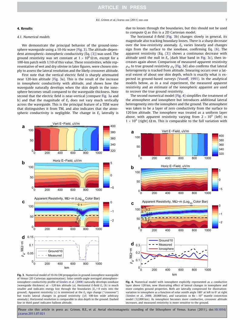
We demonstrate the principal behavior of the ground-iono-sphere waveguide using a 10-Hz wave (Fig. 3). The altitude-depen-dent atmospheric–ionospheric conductivity (Eq. (3)) was used. Theground resistivity was set constant at 1 � 106 X m, except for a100-km patch with 1/10 of this value. These resistivities, while rep-resentative of wet and dry olivine in later figures, were chosen sim-ply to assess the lateral resolution and the likely crossover altitude.

First note that the vertical electric field is sharply attenuatednear 120-km altitude (Fig. 3a). This is the result of the increasein ionospheric conductivity with altitude, and shows how thewaveguide naturally develops when the skin depth in the iono-sphere becomes small compared to the waveguide thickness. Notesecond that the electric field is near-vertical (compare Fig. 3a andb) and that the magnitude of Ez does not vary much verticallyacross the waveguide. This is the principal feature of a TEM wavethat distinguishes it from TM, and also indicates that the atmo-spheric conductivity is negligible. The change in Ez laterally is

Vert E−Field, uV/m

0 200 400 600 800 10000

50

100

320

340

360

380

400

Horiz E−Field, uV/m

0 200 400 600 800 10000

50

100

−5

0

5

Apparent Resistivity, MΩ−m (Log10 Color Bar)

0.50.20.1

0.010.01

0.1

0 200 400 600 800 10000

50

100

−2

−1

0

0 200 400 600 800 10000

0.05

0.1

0.15

km

ρ a, MΩ

−m

Ground/10Measured

a

b

c

d

Fig. 3. Numerical model of 10-Hz EM propagation in ground-ionosphere waveguideof Venus (2D Cartesian approximation). Solar-zenith-angle-averaged atmosphere–ionosphere conductivity profile of Simões et al. (2008) naturally develops ionobase(waveguide thickness) at �120 km altitude (a). Horizontal E-field Ex (b) is muchsmaller and indicates energy lost through the boundaries (Ex > 0 exits into theground). Apparent resistivity (c) is minimized at the Ex sign change (‘‘crossover’’)but tracks lateral changes in ground resistivity ((d) 100-km wide arbitraryanomaly). Horizontal resolution is comparable to skin depth in the ground. Dashedline in third panel indicates balloon altitude.


due to losses through the boundaries, but this should not be usedto compute Q as this is a 2D Cartesian model.

The horizontal E-field (Fig. 3b) changes slowly in general, itsmagnitude also tracking boundary losses. There is a sharp decreaseover the low-resistivity anomaly. Ex varies linearly and changessign from the surface to the ionobase, confirming Eq. (6). Theapparent resistivity (Eq. (3)) shows a continuous decrease withaltitude until the null in Ex (dark blue band in Fig. 3c), then in-creases again above. Comparison of measured apparent resistivityqm to true ground resistivity qg (Fig. 3d) also confirms that lateralheterogeneity is tracked from altitude. Smearing occurs over a lat-eral extent of about one skin depth, which is exactly what is ex-pected in ground-based surveys (Vozoff, 1991). In the analyticalmodels below, as in a real experiment, the measured apparentresistivity and an estimate of the ionospheric apparent are usedto recover the true ground resistivity.

The second numerical model (Fig. 4) simplifies the treatment ofthe atmosphere and ionosphere but introduces additional lateralheterogeneity into the ionosphere and the ground. The atmospherewas taken to be a layer of zero conductivity from the surface to120 km altitude. The ionosphere was treated as a uniform layerabove, with apparent resistivity varying from 2 � 105 (left) to1 � 105 (right) X m. This is comparable to the full variation with

Vert E−Field, uV/m

0 200 400 600 800 10000

50

100

Horiz E−Field, uV/m

0 200 400 600 800 10000

50

100

Apparent Resistivity, MΩ−m (Log10 Color Bar)

10.5

0.20.10.010.010.10.20.50.5

0 200 400 600 800 10000

50

100

0 200 400 600 800 10000

0.1

0.2

0.3

km

ρ a, MΩ

−m

320340360380400

−5

0

5

−2

−1

0

Ground/10MeasuredIonosphere

a

b

c

d

Fig. 4. Numerical model with ionosphere explicitly represented as a conductivelayer above 120 km, now illustrating effect of lateral changes in ionosphere andmore complex ground properties. Both are laterally compressed for illustration:variation in ionosphere as a function of solar zenith angle 180� at left to 0� at right(Simões et al., 2008; 20,000 km), and variations in Ra � 103 mantle convectionmodel (12,000 km). As ionosphere becomes more conductive, crossover altitudeincreases, and measured resistivity is more sensitive to the ground.





SZA suggested by Simões et al. (2008), but squeezed horizontallyinto 1000 km for illustration. Similarly, the apparent resistivityacross 10,000 km of convection model at Ra � 103 was computedusing the dry olivine law and squeezed into the 1000-km horizon-tal extent of the displayed EM model. The results are qualitativelysimilar to the previous model. The electric field is still very nearlyvertical, but some deflection is evident in both the verticallychanging strength of Ez (Fig. 4a) and the variability in Ex (Fig. 4b).The altitude of the Ex crossover and qm minimum (Fig. 4c) increasesfrom left to right because ionospheric resistivity is decreasing(Fig. 4d), pulling the ionospheric anchor point (Fig. 2) closer tozero. The measurement is everywhere below the crossover in thisexample, but the apparent resistivity is seen to reflect the proper-ties of both the ground and the ionosphere (Fig. 4d).

These numerical models confirm the analytic derivation thatmeasurements of TEM waves from balloon altitude on Venus aresensitive to the properties of both the ionosphere and the subsur-face, with the altitude variation a simple function of the boundaryproperties. The 2D models also show that lateral resolution is<100 km, a sufficiently long distance to allow signal integrationwithin a resolution element, but small compared with surfacescales of mantle convection.

4.2. Analytical models

The effects of a crust and mantle water on conductivity and theaerial measurement procedure to recovering lithospheric thicknesswere tested using the analytical model described above.

Reference models with specified L = 100–500 km (linear tem-perature gradients), for wet and dry olivine conductivity, areshown in Fig. 5. The asymptotic depth mapping of the first four

3 4 5 6 7 8

0

25

50

75

100

125

150

Nominal Point Measurement

Log10 Resistivity, Ω−m

Dep

th, k

m

Fig. 5. Dry (solid) and ‘‘wet’’ (dashed) electrical resistivity vs. depth for specifiedlithospheric thicknesses of L = 100–500 km at 100-km increments (red throughgray, respectively). Symbols show resistivity structure inverted at the first fourSchumann resonances (�10 to �32 Hz; lowest frequency penetrates deepest). Errorellipses at representative L = 300 km and 1st and 4th resonances indicate effect ofnominal instrumental errors on resistivity-depth recovery. Random errors arelarger for wet resistivity due to smaller induced fields. These calculations representpoint measurements without horizontal averaging. (For interpretation of thereferences to color in this figure legend, the reader is referred to the web versionof this article.)


Schumann resonances onto these resistivity structures are shownas symbols. With no biases, the recovered resistivities match thetrue resistivities. The ellipses show representative measurementerrors using the nominal electrometer. Errors are small for dry oliv-ine because Ex is large at high resistivity, and lithospheric thicknessappears to be adequately resolved (this is formalized below as esti-mated thermal gradient and errors). Conversely, the low resistivityof the wet olivine decreases (Ex/rE)2 to the point where lithospher-ic thickness is not well-resolved.

The reference case is hardly changed by inclusion of a 30-kmthick, conductive crust (Fig. 6). The Schumann resonances gener-ally penetrate to much greater depths in the dry cases and so areinsensitive to the crust. If the lithosphere is as thin as 100 km thereis some distortion. The dry-olivine resistivities are still sufficientlyhigh that errors are not affected. The errors compound for wet oliv-ine, but this is immaterial because L cannot be recovered anyway.Note that this modeled wet, conductive crust for Venus is only nowmoving into the realm of poorly conducting rocks on Earth.

Aerial soundings, including random variations and bias of theionosphere as well the quadrature bias, are shown in Fig. 7. Twoinversions (sets of symbols) are indicated for each specified litho-sphere, with the ionospheric resistivity double and half the ex-pected value. These resistivities therefore fall on opposite sides ofthe true resistivity curves. For dry olivine, the bias suggests thatL can still be reasonably estimated. However, the decrease in Ex

with altitude now also decreases (Ex/rE)2, and the ionospheric ran-

dom errors also contribute, so that the accuracy on L degrades. Themeasurement accuracy improves the estimate of L when the largeelectrometer is introduced (dotted ellipses). Biases in the wet-oliv-ine cases strongly shift the recovered curves or even cause theresistivity to diverge from a monotonic decrease with depth. Therandom errors have also increased.

These tests were repeated using results extracted from thenumerical models of mantle convection. The added value is an esti-mate of the variability about a mean lithospheric thickness L. Fig. 8

3 4 5 6 7 8

0

25

50

75

100

125

150

Conductive Crust


Dep

th, k

m

Fig. 6. Effect of electrically conductive 30-km crust on EM point inversion.Systematic error occurs only where Schumann depth sensitivity smears crust–mantle boundary. Random errors remain modest for dry resistivity, but degradefurther for wet resistivity.




3 4 5 6 7 8

0

25

50

75

100

125

150

Airborne Measurement With Ionosphere


Dep

th, k

m

Fig. 7. Effect of airborne measurement on EM inversion. This model includes biasmultipliers of ½ and 2 in the noon-to-midnight ionospheric resistivity as well as a50% local random variation. There are two inversions (sets of symbols) for eachcurve to cover the bias range. Random errors increase due to the smaller inducedfields measured at the balloon altitude (see text). Finally, only the quadraturecomponent is used to reconstruct the induced field: this obviates the need todeconvolve the reference field but it introduces an additional bias. The dotted errorellipses introduce a large electrode configuration using the interior surface of theballoon for improved measurement accuracy (see Appendix).

3 4 5 6 7 8

0

25

50

75

100

125

150

175

200

Convection Models


Dep

th, k

m

Fig. 8. Point soundings for convection models. Red, green, and blue correspond toRayleigh numbers = 104, �103, and 102, respectively. Error ellipses are for nominalmeasurement. The selected profiles for each model are representative of the meanand standard deviation but are actual. Compare to Fig. 5. (For interpretation of thereferences to color in this figure legend, the reader is referred to the web version ofthis article.)



plots representative resistivity-depth curves for wet and dry oliv-ine for the three convection models (Ra = 102, �103, and 104).These are individual points from the model but were chosen tobe representative of the mean plus/minus one standard deviation.Note that the variability increases as Ra increases and L thins. Thereference model (Fig. 8) again shows good recovery for dry olivineand poor results for wet olivine. The crust (Fig. 9) has no effect on

3 4 5 6 7 8

0

25

50

75

100

125

150

175

200

Convection Models w/ Crust


Dep

th, k

m

Fig. 9. Point soundings for convection models with conductive crust superimposed.Compare to Fig. 6.

3 4 5 6 7 8

0

25

50

75

100

125

150

175

200

Convection Models w/ Iono


Dep

th, k

m

Fig. 10. Point soundings for convection models with aerial-measurement effects(ionosphere and quadrature bias). Large errors for wet ground conductivities notshown. Compare to Fig. 7.




Table 1Point measurement accuracy of lithospheric thermal gradient.

Mantle conductivity Dry Dry Dry Dry Wet Wet Wet WetIonosphere error? No Yes No Yes No Yes No YesConductive crust? No No Yes Yes No No Yes Yes

True dT/dz, K/km (L, km) Inferred dT/dz and standard error9.5 (100) 9.5 ± 5.8 (2.4) 7.1 ± 39 (13) 4.0 ± 37 (37) NR 8.4 ± 13 (2.0) NR 9.4 ± 29 (2.2) NR4.8 (200) 5.0 ± 2.0 (1.1) 5.2 ± 6.6 (3.9) 4.7 ± 3.2 (2.8) 4.5 ± 8.2 (7.2) 4.6 ± 5.2 (0.7) NR 4.6 ± 43 (41) NR3.2 (300) 3.3 ± 1.1 (0.7) 3.4 ± 3.2 (1.9) 3.3 ± 1.1 (0.6) 3.3 ± 3.6 (2.8) 3.1 ± 3.1 (0.4) NR NR NR2.4 (400) 2.5 ± 0.7 (0.5) 2.6 ± 1.9 (1.2) 2.5 ± 0.7 (0.4) 2.4 ± 2.1 (1.7) 2.3 ± 2.2 (0.3) NR NR NR1.9 (500) 2.0 ± 0.5 (0.4) 2.1 ± 1.3 (0.9) 2.0 ± 0.5 (0.3) 2.0 ± 1.4 (1.2) 1.8 ± 1.7 (0.3) NR NR NR

L = Lithospheric thickness: uniform thermal gradient from 740 to 1690 K over depth L.NR = no result (failed inversion or extreme error).Errors reported for nominal electrometer; numbers in parentheses use optimal electrometer.

Table 2Ensemble measurement accuracy of lithospheric thermal gradient.

Mantle conductivity Dry Dry Dry Dry Wet Wet Wet WetIonosphere error? No Yes No Yes No Yes No YesConductive crust? No No Yes Yes No No Yes Yes

True dT/dz, Std. Dev., K/km Inferred dT/dz and standard error4.1 ± 1.0 (Ra = 104) 4.3 ± 1.0 4.6 ± 1.1 4.1 ± 0.9 3.9 ± 0.8 4.0 ± 1.1 5.1 ± NR 4.5 ± 0.5 NR2.6 ± 0.4 (Ra ffi 103) 2.8 ± 0.3 2.9 ± 0.3 2.8 ± 0.3 2.8 ± 0.3 2.6 ± 0.3 3.4 ± NR 4.1 ± 0.1 NR1.2 ± 0.1 (Ra = 102) 1.4 ± 0.1 1.4 ± 0.1 1.4 ± 0.1 1.4 ± 0.1 1.3 ± 0.1 2.0 ± NR 5.2 ± 0.1 NR

Ra = Rayleigh number.NR = no result (failed inversion or extreme error).


these models (because the thinnest L = 250 km). The aerial mea-surement (Fig. 10) for wet olivine again fails to provide usefulinferences about L. Even with bias and the small electrometer,these cases can be distinguished for dry olivine.

Such interpretation of Figs. 8–10 still treats the results as pointmeasurements. We are interested in comparing these point esti-mates to the large-scale lateral averages afforded by the convec-tion models. Tables 1 and 2 give the geothermal gradients foreach of the lithospheric models used in this paper (actual for spec-ified lithospheres, mean for convection models) and the estimatedvalues and errors from Section 3.7. These results also span all 8combinations of conductivity law and effect of crust or ionosphere.The best-case accuracies for the reference point measurements inthe range of expected lithospheric thicknesses for Venus are 20–30%. However, the accuracy on thermal gradient degrades to�100% or worse when the airborne measurement is treated. The513 grid points in the convection models provide an equal numberof measurement stations, so the average thermal gradient on theprofile can be improved by averaging. We find that for all caseswith dry olivine, the standard deviation of the estimated thermalgradient is comparable to the standard deviation of the data,<25%. The nominal electrometer is sufficient for this purpose. Thedifficulties in measuring the small electric fields induced in wetolivine preclude assessment of errors on thermal gradient and inthe worst cases no estimate is obtained at all.

The standard deviation of the mean estimated thermal gradientis of course smaller by

p513, in which case the net error on geo-

thermal gradient is dominated by the bias or offset between theestimated and true values, typically �10% in Table 2.

5. Concluding discussion

We have developed a comprehensive, but still exploratory, con-ceptual framework for EM sounding of the lithosphere of Venus.We found that lightning-caused Schumann resonances are capableof penetrating 50–100 km in a dry Venus, thus investigating adepth interval sensitive to vertical temperature changes. This al-lows estimation of lithospheric thickness or thermal gradient.


The presence of hundreds of ppm H2O will increase conductivityenough so that the vertical length scale is limited to <20 km. This,and the decrease in measurement SNR, precludes robust estima-tion of lithospheric properties. The presence of significant waterin the crust of Venus could nonetheless be inferred, and variationsin shallow structure tracked.

The higher SNR in a three-component electrometer composedof orthogonal booms is superior to using a two-component elec-trometer and a magnetometer. Even if the vertical electrode sepa-ration is restricted to �1 m, the SNR in measuring the verticalelectric field as the reference is still much greater than using thehorizontal magnetic field. A large electrode area and tip separationare important for obtaining good measurements of the horizontalelectric field. Using the balloon itself is the optimal solution toobtaining high E-field SNR (Appendix).

We have shown that aerial EM sounding on Venus is really ajoint investigation of the subsurface and ionosphere. With long tra-verses (�104 km), mean properties of the ionosphere and subsur-face can be recovered. Joint regional (�103 km) inversion may bepossible with additional constraints, e.g., the variation of the iono-spheric resistivity with SZA and recognition that the ground resis-tivity will be correlated at long wavelength with topography (bothare correlated with temperature). Local (�102 km) solutions(essentially point measurements) may provide useful tiepoints ifthe ionospheric resistivity can be estimated from distortion inthe balloon downlink.

The data processing follows the usual hierarchy, with associatedincreasing sophistication of interpretation. The complex spectraform the Level 1 data (likely available data rates from a balloon willnot permit return of raw time series: onboard spectral estimationis necessary). Solution of EM measurements for resistivity vs.depth forms Level 2 data. Such data are useful for confirming thepredicted vertical and horizontal trends expected for the increaseof temperature with depth and the larger thermal anomalies overvolcanic rises. Thickened crust over plateau (tessera) highlandswould also be evident. Level 3 data follow from the final step de-scribed here, estimation of thermal gradient.

The electric-field measurements required for aerial EM sound-ing on Venus are closely related to those used in space- and atmo-





spheric-physics investigations, onboard processing can returncompact but useful data, and long traverses can separate groundand ionospheric contributions. The general approach describedcan be implemented for high-altitude (20 km) surveying on Earthand ionospheric conductivity can be estimated from GPS-signal de-lay. If Mars or Titan have lightning, they too will likely have Schu-mann resonances, and can be electromagnetically probed fromaerial vehicles.

Acknowledgments

This research was supported by SwRI IR&D Project R8043 andby NASA Grant NNX07AP27G. We are grateful to two anonymousreviewers, one of whom substantially changed the trajectory ofthe paper by pointing out more recent experiments on the conduc-tivity of hydrous olivine.

Appendix A. Spherical-octant electrode configuration

We have developed a novel electrode design suitable for wave-tilt measurements from a balloon. All ‘‘electrically small’’ measure-ments depend critically on two parameters: the capacitive reac-tance Z of the sensors and their ‘‘effective’’ separation Dx.Because Z = 1/xC, where x is the angular frequency and C is thecapacitance, it is essential to increase capacitance as frequency isdecreased in order to maintain a given noise level in the amplifier.C is nearly a linear function of electrode size. The signal DV in-creases linearly with Dx (because E ffi DV/Dx). Therefore the sig-nal-to-noise ratio (SNR) increases with C and Dx.

Prior aerial electric-field measurements have used parallel orcurved plates, small spheres or cylinders separated by booms, orlimited surfaces on a sphere. Each of these geometries has a draw-back in small capacitance, small effective separation, or inability tomeasure three spatial components of the electric field.

Our electrode array (Fig. A1) is nearly optimal for low-frequencyballoon measurements, in that it:

1. Is a minimum-volume configuration by using the surface of asphere.

2. Maximizes capacitance by using nearly 50% of the available sur-face area.

Fig. A1. Spherical octant electrode design for aerial E-field measurement. Byalternately joining the electrodes in pairs and differencing with the complementarypair, three spatial components are recovered. This configuration maximizescapacitance and effective antenna length and minimizes volume and self-interfer-ence. Computational mesh is superimposed.


3. Maximizes electrode separation by differencing voltages acrossopposing hemispheres (the small separations at the cornershave little effect because the affected area is small).

4. Is able to measure three spatial components of the field byalternately joining pairs of electrodes and differencing themwith the opposing pair. In this way only four electrodes arerequired where normally six would be used.

Through numerical modeling, we determined that C ffi 76a pFand Dx ffi 0.7a, where a is the sphere radius in meters. These rela-tions assume the corner gap is �a. There are several additionalbenefits to this design that optimize its incorporation into a bal-loon hull:

5. The electrodes can be sufficiently thin so as not to substantiallyimpact balloon mass.

6. The electrode flexibility and configuration along the gore direc-tion will make them easy to build into the balloon hull and notaffect deployment or flight performance.

7. The cable bundle containing the attachment leads running fromthe top to bottom of the balloon can be incorporated with exist-ing structural/signal lines. The entire line can be actively drivento make it electrically ‘‘invisible.’’

The voltages on the individual electrodes must be amplified anddifferenced (and digitized) to produce an E-field measurement. Wehave designed the relevant circuitry based on the OPA129 op-amp.For a 6-m balloon, the predicted sensitivity at 10 Hz is better than50 pV/m/

pHz.

We note finally that the measurements claimed in a 2004 USpatent by Barringer (#6,765,383) at frequencies less than hundredsof hertz (indeed, down to <1 Hz) are physically impossible due tothe small size and spacing of the electrodes.

References

Arcone, S., 1978. Investigation of a VLF airborne resistivity survey conducted innorthern Maine. Geophysics 43, 1399–1417.

Arkani-Hamed, J., 1994. On the thermal evolution of Venus. J. Geophys. Res. 99,2019–2033.

Barringer, A.R., 1973. Geophysical exploration method using the vertical electriccomponents of a VLF field as a reference, U.S. Patent, Nr. 3594,633.

Bevington, P.R., 1969. Data Reduction and Error Analysis for the Physical Sciences.McGraw-Hill, New York, 336pp.

Bolfan-Casanova, N., 2005. Water in the Earth’s mantle. Mineral. Mag. 69, 229–257.Borucki, W.J. et al., 1982. Predicted electrical conductivity between 0 and 80 km in

the venusian atmosphere. Icarus 51, 302–321.Bostick, F.X., 1977. A simple almost exact method of magnetotelluric data analysis.

Proc. Workshop on Electrical Methods in Geothermal Exploration, Univ. Utah.Brace, L.H., Kliore, A.J., 1991. The structure of the Venus ionosphere. Space Sci. Rev.

55, 81.Brace, L., Elphic, R., Curtis, S., Russell, C., 1983. Wave structure in the Venus

ionosphere downstream of the terminator. Geophys. Res. Lett. 10, 1116–1119.Bullock, M.A. et al., 2009. Venus flagship mission study: Report of the Venus science

and technology definition team. JPL.Constable, S., 1993. Constraints on mantle electrical conductivity from field and

laboratory measurements. J. Geomag. Geoelectr. 45, 707–728.Constable, S., Shankland, T.J., Duba, A., 1992. The electrical conductivity of an

isotropic olivine mantle. J. Geophys. Res. 97, 3397–3404.Egbert, G.D., Booker, J.R., 1992. Very long period magnetotellurics at Tucson

Observatory: Implications for mantle conductivity. J. Geophys. Res. 97, 15099–15112.

Grebowsky, J.M., Strangeway, R.J., Hunten, D.M., 1997. Evidence for Venus lightning.In: Boucher, S.W. et al. (Eds.), Venus II. Univ. Arizona Press, Tucson, pp. 125–157.

Grimm, R.E., 2002. Low-frequency electromagnetic exploration for groundwater onMars. J. Geophys. Res. 107. doi:10.1029/2001JE001504.

Grimm, R.E., 2009. Electromagnetic sounding of solid planets and satellites. NRCWhite Paper. <www8.nationalacademies.org/ssbsurvey/publicview.aspx>.

Grimm, R.E., Hess, P.C., 1997. The crust of Venus. In: Boucher, S.W. et al. (Eds.),Venus II. Univ. Arizona Press, Tucson, pp. 1205–1244.

Grinspoon, D.H., 1993. Implications of the high D/H ratio for the sources of water inVenus’ atmosphere. Nature 363, 428–431.

Jones, A.G., Ferguson, I.J., 2001. The electric Moho. Nature 409, 331–333.


http://dx.doi.org/10.1029/2001JE001504

http://www8.nationalacademies.org/ssbsurvey/publicview.aspx




Karato, S., 2006. Remote sensing of hydrogen in the Earth’s mantle. Rev. Mineral.Geochem. 62, 343–375.

Kaula, W.M., Phillips, R.J., 1981. Quantitative tests for plate tectonics on Venus.Geophys. Res. Lett. 8, 1187–1190.

Lizarralde, D., Chave, A., Hirth, G., Schultz, A., 1995. Northeastern pacific mantleconductivity profile from long-period magnetotelluric sounding using Hawaii-to-California submarine cable data. J. Geophys. Res. 100, 17837–17854.

Lognonné, P., Occhipinti, G., Garcia, R., 2005. Seismic interior/atmosphere couplingon Venus. Lunar Planet. Sci. XXXVI. Abstract 2274.

McNeill, J.D., 1990. Use of electromagnetic methods for groundwater studies. In:Ward, S.H. (Ed.), Geotechnical and Environmental Geophysics, vol. 1. Society ofExploration Geophysicists, Tulsa, pp. 191–218.

McNeill, J.D., Labson, V.F., 1991. Geological mapping using VLF radio fields. In:Nabighian, M.N. (Ed.), Electromagnetic Methods in Applied Geophysics, vol. 2.Society of Exploration Geophysicists, Tulsa, pp. 521–640.

Moore, W.B., Schubert, G., 1997. Venusian crustal and lithospheric properties fromnonlinear regressions of highland geoid and topography. Icarus 128, 415–428.

Moresi, L.-N., Solomatov, V.S., 1995. Numerical investigation of 2D convection withextremely large viscosity variations. Phys. Fluids 7, 2154–2162.

Namiki, N., Solomon, S.C., 1995. Degassing of argon, helium, and water and thenature of crustal formation on Venus. Lunar. Planet. Sci. XXVI, 1029–1030(abstract).

Nickolaenko, A.P., Hayakawa, M., 2002. Resonances in the Earth-Ionosphere Cavity.Kluwer, Dordrecht, 380pp.

Nickolaenko, A.P., Rabinowicz, L.M., 1982. On the possibility of existence of globalelectromagnetic resonances on the planets of the Solar System. Space Res. 20,82–89.

Pechony, O., Price, C., 2004. Schumann resonance parameters calculated with apartially uniform knee model on Earth, Venus, Mars, and Titan. Radio Sci. 39.doi:10.1029/ 2004RS003056.

Phillips, R.J., Malin, M.C., 1983. The interior of Venus and tectonic implications. In:Hunten, D.M. et al. (Eds.), Venus. Univ. Arizona Press, pp. 159–214.

Phillips, R.J. et al., 1997. Lithospheric mechanics and dynamics on Venus. In:Boucher, S.W. et al. (Eds.), Venus II. Univ. Arizona Press, Tucson, pp. 1163–1204.

Poe, B.T., Romano, C., Nestola, F., Smyth, J.R., 2010. Electrical conductivityanisotropy of dry and hydrous olivine at 8 GPa. Phys. Earth Planet. Inter. 181,103–111.

Roux, A. et al., 2008. The search coil magnetometer for THEMIS. Space Sci. Rev. 141,265–275.

Russell, C.T. et al., 2007. Lightning on Venus inferred from whistler-mode waves inthe ionosphere. Nature 450, 661–662.

Russell, C.T., Zhang, T.L., Wei, H.Y., 2008. Whistler mode waves from lightning onVenus: Magnetic control of ionospheric access. J. Geophys. Res. 113.doi:10.1029/2008JE003137.

Sagdeev, R.Z., Linkin, V.M., Blamont, J.E., Preston, R.A., 1986. The VEGA Venusballoon experiment. Science 231, 1407–1408.


Schubert, G., Solomatov, V.S., Tackley, P.J., Turcotte, D.L., 1997. In: Boucher, S.W.et al. (Eds.), Venus II. Univ. Arizona Press, Tucson, pp. 1245–1287.

Schubert, G., Turcotte, D.L., Olson, P., 2001. Mantle convection in the Earth andplanets. Cambridge Univ. Press, 940pp.

Simões, F. et al., 2008. Electromagnetic wave propagation in the surface-ionospherecavity of Venus. J. Geophys. Res. 113. doi:10.1029/2007JE003045.

Simpson, F., Bahr, K., 2005. Practical Magnetotellurics. Cambridge Univ. Press,254pp.

Sjogren, W.L. et al., 1997. The Venus gravity field and other geodetic parameters. In:Boucher, S.W. et al. (Eds.), Venus II. Univ. Arizona Press, Tucson, pp. 1125–1161.

Solomatov, S., 1995. Scaling of temperature- and stress-dependent viscosityconvection. Phys. Fluids 7, 266–274.

Solomatov, V.S., Moresi, L.-N., 1996. Stagnant lid convection on Venus. J. Geophys.Res. 101, 4737–4753.

Solomon, S.C., Head, J.W., 1982. Mechanisms for lithospheric heat transport onVenus: Implications for tectonic style and volcanism. J. Geophys. Res. 87, 9236–9246.

Solomon, S.C. et al., 1992. Venus tectonics: An overview of Magellan observations. J.Geophys. Res. 97, 13199–13255.

Telford, W.M., Geldart, L.P., Sheriff, R.E., 1990. Applied Geophysics, second ed.Cambridge Univ. Press, 770pp.

Turcotte, D.L., 1993. An episodic hypothesis for venusian tectonics. J. Geophys. Res.98, 17061–17068.

Turcotte, D.L., 1995. How does Venus lose heat? J. Geophys. Res. 100, 16931–16940.Vozoff, K., 1991. The magnetotelluric method. In: Nabighian, M.N. (Ed.),

Electromagnetic Methods in Applied Geophysics, vol. 2. Society of ExplorationGeophysicists, Tulsa, pp. 641–711.

Wait, J.R., 1970. Electromagnetic waves in stratified media, Pergamon.Wang, D., Mookherjee, M., Xu, Y., Karato, S., 2006. The effect of water on the

electrical conductivity of olivine. Nature 443, 977–980.Wight, D.E., Bostick, F.X., 1980. Cascade decimation – A technique for the real time

estimation of power spectra. IEEE Int’l Conf. Acoustic Speech and Signal Proc.,pp. 626–629.

Wilson, C.F. et al., 2011. The 2010 European Venus Explorer (EVE) mission proposal:The first in situ circumnavigation of an alien world. Exp. Astron., submitted forpublication.

Wittall, K.P., Oldenburg, D.W., 1992. Inversion of magnetotelluric data for a one-dimensional conductivity. Geophys. Monogr. Ser. 5. Society of ExplorationGeophysicists, Tulsa, 114pp.

Xu, Y., Shankland, T.J., Poe, B.T., 2000. Laboratory-based electrical conductivity inthe Earth’s mantle. J. Geophys. Res. 105, 27865–27875.

Yoshino, T., Matsuzaki, T., Shatskiy, A., Katsura, T., 2009. The effect of water on theelectrical conductivity of olivine aggregates and its implications for theelectrical structure of the upper mantle. Earth Planet. Sci. Lett. 288, 291–300.


http://dx.doi.org/10.1029/2004RS003056

http://dx.doi.org/10.1029/2008JE003137

http://dx.doi.org/10.1029/2007JE003045



aerial electromagnetic sounding of the lithosphere …dstillman/pdf/grimm_icarus_2011pip.pdf ·...

Documents