adventures in applied mathematics

QUARTERLY OP APPLIED MATHEMATICS 67

APRIL, 1972

SPECIAL ISSUE: SYMPOSIUM ON"THE FUTURE OF APPLIED MATHEMATICS"

ADVENTURES IN APPLIED MATHEMATICS

C, L. PEKERIS

The Weizmann Institute

Rehovot, Israel

Abstract. A review is given of the work carried out at the Weizmann Institute

during the past 25 years in the fields of terrestrial spectroscopy, the dynamo theory

of the earth's magnetic field, the tides in the world oceans, theoretical seismograma,

hydrodynamic stability, atomic spectroscopy, and the Boltzmann integral equation.

Some open problems in the solution of the Schrodinger wave equation are formulated.

1. Introduction. On May 15, 1946, at about the time of the founding of the Division

of Applied Mathematics at Brown, an international symposium was held in Rehovot,

Israel, on the occasion of the laying of the cornerstone of the Weizmann Institute.

In my talk, entitled "Some unsolved problems in classical physics," I dealt* with the

following topics:

(1) Pulsation theory of Cepheid variables;

(2) Equatorial acceleration of the sun;

(3) Origin of the earth's magnetic field;

(4) Problems of atmospheric tides and related geophysical phenomena;

(5) Theory of reflection of light or of sound from a rough surface;

(6) Problem of hydrodynamic stability.

I should like now to take stock and examine to what extent we succeeded in solving

some of these problems. Then I shall proceed to topics of more recent origin. The dis-

cussion will be based on our own work at the Weizmann Institute, which was aimed at

the solution of outstanding problems in the physical sciences.

2. Terrestrial spectroscopy. The brightness of some 5% q( all stars is variable,

and in many cases the variation is strictly periodic in time. A concomitant periodicity

is also observed in the radial velocity, suggesting that the phenomenon is due to a

radial pulsation of the star. The pulsation theory predicts that the period of radial

pulsation is of the order of the time it takes for a sound wave to travel from the center

to the surface of the star—thus providing us with information on the mean temperature

inside the star.

Today we know that our planet earth also goes into a radial pulsation when per-

turbed by a strong enough earthquake. This radial pulsation was observed for the

first time in the seismic and gravimetric records of the Great Chilean Earthquake of

May, 1960. Fig. 1 shows the spectral peaks of the free oscillations of the earth deduced

by Professor Slichter's group [1] from their gravimetric record of the Chilean earthquake.

The peak marked 54 min. is the fundamental spheroidal oscillation, corresponding

* Trends in modern science, Interscience, New York, 1949, pp. 211-226.

68 C. L. PEKERIS

10-UMFILTERED SPECTRUM DISTURBED INTERVAL 110 HOURS

|0I32 MAY 23 TO I52» MAY 27 INO

BMT)

I 2 3 4 5 6 7 8 9 10 II 12 13 14 15FREQUENCY- CYCLES / HOUR

20 21 22 23 24 25FREQUENCY - CYCLES / HOUR

Fia. 1. Power spectrum of gravity record after Chilean earthquake (May 22, 1960) in comparison

with that for corresponding quiet period. [1],

to a spherical harmonic of order n = 2. The radial pulsation mode, with n = 0, has a

theoretical period [2] of around 20.5 min., depending on the model assumed for the earth.

The observed peak is the one marked 20 in the figure. The second curve shows the

spectrum of the gravimetric record made a month after the Chilean earthquake. All

the spectral lines have decayed, except the purely radial pulsation peak marked 20.5.

1960 saw the birth of the new science of terrestrial spectroscopy [3], and currently

attention is centered on the radial pulsation mode and its overtones.

The mathematical problem arising in terrestrial spectroscopy is as follows: The

model of the earth is prescribed by specifying the distribution of the elastic constants

X(r) and n(r) and of the equilibrium density p0(r). From the density alone we can deter-

ADVENTURES IN APPLIED MATHEMATICS 69

mine the distribution of the equilibrium force of gravity g0(r). In the case of a purely

radial pulsation, the displacement u{r) is governed by the equation

2,4 dpo<x u i— p0goU + ~r

r ar X(" + ~V) + + r (4" ~~ ̂f) ~~ °' (1)

subject to the boundary condition

(X + 2y)u + - \u = 0, r = a. (2)r

Here a denotes the eigenfrequency of the model for a purely radial pulsation.

In the second class of a purely toroidal mode, the displacements, in a spherical system

of coordinates, are defined as

u = 0, v = dSn[9' ^ e", w = — f/(r) —e'", (3)sin 6 d<p ou

with U(r) satisfying the equation

subject to the boundary condition

(dU/dr) - (U/r) = 0, r = a. (5)

The solution of both Eqs. (1) and (4) is a trivial matter, except for the need to dif-

ferentiate the empirically-determined elastic functions X(r) and ju(r). This difficulty

can be avoided by using the stresses as unknowns, instead of the displacements, as will

be explained below.

In the third, and more difficult, class of oscillations, that of the poloidal modes,

the motion is governed not only by elastic forces but also by gravitational forces arising

from the change in the density field brought about by the oscillation. The displacements

now depend on two functions, U(r) and 7(r):

u = U(r)Sn(0, 4>), V = F(r) dS"(^ , w = ^j(6)

The perturbation in the gravitational field \p and the dilatation A are represented by

A = X(r)Sn(d, $), V = P(r)Sn(6, <t>), (7)

with

X = U + (2/r)U - [n(n + 1 )/r]V. (8)

The unknown functions U(r), V(r) and P(r) are subject to the differential system of

the sixth order

a2PoU + PoP + goPoX - p0 j- (g0U) + ~ (XX + 2Mt/)

(9)

+ % [4Ur -4U + n(n + 1)(-U - rV + 37)] = 0,r

70 C. L. PEKERIS

Po<r2Fr + p0P — gop0U + \X + r jj;

(10)

+ - [5U + 3rV - V - 2n(n + 1)7] = 0,r

p + _ n(n + l)p = AtG(.oU + poZ)j (n)r r

In order to obviate the need for differentiating the empirically-determined elastic

parameters X(r) and n(r) we introduce as new variables

2/i = U, y2 = XX + 2pt7, y3 = V, (12)

y4 = - 7 + 7) , 2/5 = P, y«=P~ ±ttGPoU. (13)

In the ensuing equations, the derivatives of X(r) and /u(r) no longer appear explicitly:

... = , 2/2 , Xn(n + l)y3 , >Vl (X + 2M)r ̂ (X + 2M) + (X + 2M)r '

(15)

- PoVe

... _ r_ 2n r2 - 4 „r4. 4m(3X + 2^)1 2/i 4 [iy,y* - L 4"°^r + (X + 2/i) J r2 (X + 2/i)r

I r„/n , n iy 2m(3X + 2n)n(n + 1)1 y3 n(n + 1 )y.+ [»(» + 1 )P0g0r j ? + -

#. = -V- + ^ ^ , (16)r r \i

■ _ P 2^(3X -j- 2^)~| Xy22/4 - [ffoPor (x + 2fi) J r3(X + 2M) J r3 (X + 2p)r

{-

(17)

+ ^ ~Po<r2r2 + ^ _|_M2m) + 2n — 1) + 2p(n2 + n — 1)] j ^ — ^7^

y5 = 4tt(?po2/5 + 2/a , (18)

4xGp„y,(n + l)t/3 , n(n + 1)2/5 2j/„2/e I 7 (19)

This sixth-order differential system is to be solved subject to certain boundary conditions,

which are sufficient to determine the eigenvalue a.

These equations, which were formulated in 1958 [2], were solved by the standard

method of first expanding the solutions in the appropriate power series near the center

of the earth, and then carrying on the integration by the Runge-Kutta method. When

the first batch of data on the earth's spectrum was analyzed in 1960 it was found that

over 60 observed periods agreed to better than one percent with our theoretical values.

Today, terrestrial spectroscopy has become one of the active fields of research in geo-

physics, and has yielded new information on the internal constitution of the earth.

Historically, the subject of the earth's free oscillations was brought to the fore in

1954 when Benioff [4] reported that he had observed a period of 57 min. in the seismic

record of the Kamchatka earthquake of 1952, which he suggested might be due to a


free spheroidal oscillation of the earth. In 1911 Love [5] estimated that a homogeneous

self-gravitating earth-model would have a fundamental period of around 60 minutes.

Under Benioff's persistent persuasion we ultimately yielded, and undertook a systematic

study of the free vibrations of the real earth. It was one of the first geophysical problems

to be analyzed on the electronic computer, and served as a vehicle by which to test

and develop methods of integrating a system of ordinary differential equations.

3. The dynamo theory of the origin of the earth's magnetic field. We were lucky,

because the dynamics of the oscillations of the earth happen to be governed by a rather

stable system of equations. This is in contrast to the system of equations

A - % f. + V<1 ~ r?F* = °> (2°)r o

F2-®2F2- y{| ef\ - y [r(l - r)2Fz + (4 - 12r + 8r2)F3]} = 0, (21)

F3-%F3- f|-| [r(l - rfF, + (4 - 12r + 8r2)P\] + 2e(l - r)F4| = 0, (22)

F< - % F<

" f 1 (23)- 7|-| [3r(l - r)7\ + (-3 + 4r - r2)F\ + (-8 + 10r)F,] - 2e(l - r)f3| = 0,

which, though seemingly innocuous, turns out to be more delicate. This system of

equations arises in the dynamo theory of the origin of the earth's magnetic field. Here

you have the first major problem which will accupy applied mathematicians during the

next 25 years. I take 25 years as a yardstick because in the past 25 years this problem has

been on the books, with no impressive achievements to show. The reason, perhaps, is

that the proposed mechanism of a self-exciting dynamo in a liquid sphere (the liquid

core of the earth) is intrinsically more complex than the dynamics of the oscillations

of a gravitating elastic sphere. Indeed, a self-exciting dynamo may be impossible alto-

gether. After Larmor [6] proposed the idea of a self-exciting dynamo in 1919, it was not

until 1934 that the first reaction came from Cowling [7], who proved the negative result

that no dynamo can produce a symmetric magnetic field.

The equation governing the magnetic field H is

dH/dt = \V2H + curl (U X H). (24)

Here U denotes the velocity field, which in the kinematic approximation is assumed

to be given, and X = 1/4ttk, k denoting the electrical conductivity. Bullard and Gellman

[8] studied the steady kinematic dynamo for the case when the convection is assumed to

be represented in spherical coordinates by

ur = (Q/r*)Qs(r)Pl(cos 6) cos 2<fi, (25)

ug = [Qs(f)/r](d/dd)Pl(cos d) cos 2<f>, (26)

1 /> nn2/ M d o , QT{r) dP^COS 6)U* = V^me <2s(r)P*(c0S ^ cos 2+-—r dJ— ' (27)

Qs = r3(l - r)2, QT = er2(l - r). (28)

72 C. L. PEKERIS

The problem then reduces to an eigenvalue problem for a nondimensional parameter

V given by

V = 4iri<aU, (29)

where a denotes the radius of the sphere and U the scale of the velocity.

The system (20)-(23) is the severely truncated form of (24) when we expand H in

spherical harmonics Yn(6, <j>):

H = EF,(r)y,(M). (30)n

If we attempt a solution by expanding in power series near the origin and carrying on

thence by numerical integration, we find that, for the relevant values of the eigenvalue V

of around 50, the basic fundamental solutions grow from unity at the origin to magni-

tudes of the order of 1O10 at the surface. The equations have therefore either to be pre-

doctored or to be solved by finite-difference methods. The results achieved to date

[9, 10] are not encouraging, since they show that as the number of terms in (30) is in-

creased, the eigenvalue V grows continuously without manifesting any tendency toward

convergence. One of the immediate objectives of the dynamo theory would be to find

a steady convective field, other than the one represented by Eqs. (25)-(27), for which

the eigenvalue V does converge. If such a steady convective field exists, and at present

this is not certain, then one could turn attention to the dynamic aspects of the problem,

in particular to the mechanism which is likely to maintain the convection in the presence

of dissipation.

One such possible mechanism which I investigated recently [11] is the steady field

induced by the periodic motion in the liquid core of the earth due to the bodily tides.

The tidal potential of the moon and of the sun produce tidal motions not only in the

oceans but also throughout the body of the earth, including the liquid core. The amplitude

of the bodily tide is of the order of 20 cm. If U in (24) denotes the periodic displacement

in the liquid core of the earth due to the bodily tide, then H will also vary with the tidal

period. The cross-term curl (U X H) will produce harmonic overtones of the fundamental

tidal period, including a steady term. The magnitude of the steady term depends on

whether the induction extends through the entire body of the core, or is confined to a

skin-layer near the surface of the core. In the former case, an order-of-magnitude in-

vestigation [11] shows that the coupling between the convectively inducing and the

induced fields is too small. The question as to whether the self-exciting dynamo, if it

exists, is a body-phenomenon or a skin-effect will be elucidated only after a convergent

solution is achieved for some kinematic model.

4. The tides in the world oceans. While on the subject of tides in the core of the

earth, we cannot avoid facing up to the fact that to date the problem of determining the

tides in the ocean has not yet been solved completely. According to Laplace [12a],

one should be able to predict the amplitudes and phases of the tides f not only on the

coasts but also at every point in the interior of oceans, if we know the ocean depth

h(8, A) and if we can also solve the tidal equations

(du/dt) — 2wv cos 6 = (g/a)(df/dff) — F„ , (31)

(dv/dt) + 2com cos 6 = —(g/a sin 0)(df'/dX) — I<\ , (32)

where u and v are the components of velocity,


f = f - f, f = -n/ff, (33)

f denoting the equilibrium tide and 0 the tidal potential. The equation of continuity

fe sin ' (34)dt a sin 6 \dd d\)

together with (31) and (32), serve to determine the tide and the velocity components

u and v. The terms F$ and I'\ in (31) and (32) represent the components of the frictional

force F acting on a column of water of depth h. We found that these dissipative terms

had to be introduced; otherwise the tidal amplitudes obtained by solving the Laplace

tidal equations came out too large when compared with the observed tides on the coasts

and on islands. After tidal dissipation was introduced, the numerical stability was also

improved. The resulting tidal dissipation turned out to be of the right order of magnitude

compared with the astronomical value deduced from the observed secular acceleration

of the moon in its orbit. You may not have been aware that the day is becoming longer,

while the month and the year are becoming shorter—-all because of tidal friction. Aside

from tidal dissipation and its effect on the lunar orbit, we shall in this lecture disregard

the moon altogether.

Now in attempting to solve Laplace's tidal equations we have of course first to

determine the topography of the ocean bottom; i.e., the function h(d, X). This task is

not an attractive one to an applied mathematician, but if he aims to come to grips

with nature, he must train himself to submit to the standards of elegance set by nature,

rather than by pure mathematicians. The goal of determining, on the basis of only a given

tidal potential, the tidal motion in the huge dynamical system of the oceans covering

three-quarters of the surface of the globe, with the possibility of confronting the theoret-

ical results with numerous tidal observations as well as with observations of the asso-

ciated tidal variations in the force of gravity, should inspire the applied mathematician

to submit to the drudgery involved in determining the topography of the ocean bottom.

By now over a million ocean depth stations have been processed by Dishon [12b] from

which a representative h{6, X) can be determined.

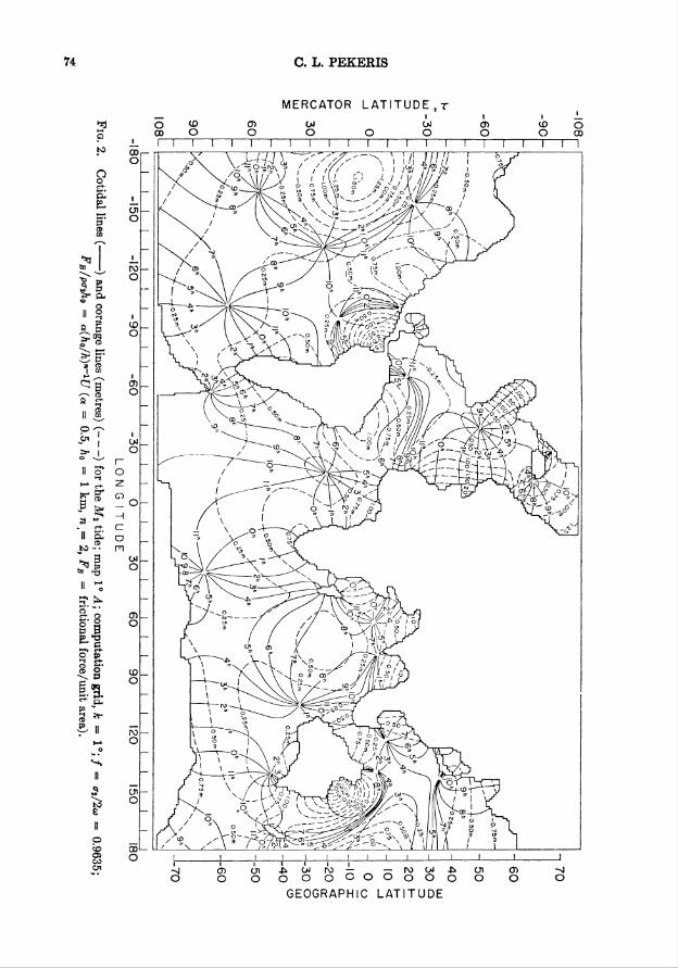
Fig. 2 shows our theoretical solution [13] of Laplace's tidal equations, modified by

the inclusion of frictional forces, for an ocean model whose coastline is defined by arcs

of 1° in latitude and longitude. The theoretical tides turned out to be of the right mag-

nitude: they could have come out in the range of kilometers or millimeters. The degree

of agreement with tidal observations is shown in Fig. 3 (facing page 78) for the Atlantic

Ocean. One of the interesting theoretical results is the existence of a South Atlantic amphi-

drome (21°S, 15°W) whose reality is supported by island observations. Further corrobora-

tion has come from Dr. Cartwright's recent tidal expedition [14] to the South Atlantic.

A great deal of additional work remains to be done by applied mathematicians

before the whole complex of tidal phenomena on the earth is understood. The significance

of this problem stems from the fact that it is the simplest dynamical system on a global

scale which we can tackle at present and from which we can gain experience which we

may hope to apply to the even more exacting task of elucidating the dynamics of our

atmosphere. The oceanic tidal problem is tied in with the bodily tide, the tides in the

atmosphere, the tide in gravity, and possibly also with the mechanism which maintains

the magnetic field of the earth. We may expect an increasing number of tidal measure-

ments in midoceanic stations, as well as a more detailed mapping of the distribution of

74 C. L. PEKERIS

MERCATOR LATITUDE,r

cr> cn uiO O OOOCOOOOO o

GEOGRAPHIC LATITUDE


tidal gravity. One of the immediate problems, both theoretically and observationally,

is tidal dissipation, which is a phenomenon confined to the shelf and coastal waters.

We have only four years left to accomplish this task before the deadline of the bicen-

tennial anniversary of the formulation of Laplace's tidal equations [12a].

5. Theoretical seismograms. Traditionally, the interpretation of seismograms was

based essentially on ray theory. Attention was centered on identifying the first arrival

times of the compressional P-wave and of the shear wave S. From the arrival times of

the P- and waves one can determine the variation of the P- and S-velocities with the

distance r from the center of the earth. In this manner, for example, Gutenberg dis-

covered that below a depth of some 3000 kilometers from the surface, the material of

the earth is liquid. The question naturally arose as to what additional information

on the structure of the interior of the earth could be gained from a study of the whole

body of the seismogram, besides the pips of the P and S arrivals. It was hoped that a

complete wave-theoretical solution for the seismic wave produced by the application of

a well-defined stress-pulse at the focus would reveal additional information on the

nature of the medium. The first theoretical seismogram was derived in 1948 [15] for the

case of an underwater explosion, and is shown in the upper part of Fig. 4. It was an

approximate solution based on the normal mode theory. This record revealed a whole

array of theoretical wave features which could be identified and measured in underwater

explosion records, and which were correlated with the structure of the bottom.

Subsequently [16a], it was possible to obtain an exact solution of the seismic wave

problem. For this purpose it was necessary first to derive an exact inversion of the

integral equation

p J exp (-pt)W(t, r, II) dt = ^ J J„(^ rxjf(x) exp [(— p/c)II(x2 + a2),/2]x dx, (35)

where f(x) is given and W is to be determined. The difficulty with (35) is that W consists

of a superposition of a series of discontinuous pulses W. , each pulse (ray) being strictly

zero until its arrival time ti , and subsequently being a well-defined function W,(t — <,).

The lower record in Fig. 4 [16b] gives the exact solution to the same underwater explosion

problem which is represented by the approximate normal-mode solution shown above.

Regrettably, no new information could be gleaned from the exact solution that had not

been derived from the earlier normal-mode solution.

6. Hydrodynamic stability. In recent years we have attacked the problem of the

stability of plane Poiseuille flow to periodic disturbances of finite amplitude. The assumed

periodicity is in the x-direction, along the axis of the main parabolic flow. Our method

was [17] to solve the Navier-Stokes equation

3V2\p | dV2* dX72ip

with

+ (36)dt dydxdxdyR

4> = to + ]C f"(y, t) exp (-iotnx), /_„ = (37)n- — oo

by letting

Uv, o = e mm®, (38)

76 C. L. PEKERIS

1—

GROUND WAVE

A

-2

BEGINNING OF GROUND WAVE

J L.05 .10 .15 .20 .25 .30

TIHB FROM BEGINNING OF GROUND WAVE, IN SECONDS

.40 .45 .50 .55

TIKE FROM BEGINNING OF GROUND WAVE, IN SECONDS

Fia. 4. Theoretical seismogram for an underwater explosion. Upper curve gives approximate normal

mode solution [15]. Lower curve gives the exact solution [16b].

where the <i>nk{y) are the solutions of the Orr-Sommerfeld equation. The aim, of course,

was to convert the partial differential equation (36) into a system of ordinary simul-

taneous differential equations for the coefficients Bnk(t), whose solution was hoped to be

more tractable. This program encountered a difficulty arising from the peculiar distri-

bution of the eigenvalues c of the Orr-Sommerfeld equation in the complex c-plane,

as shown in Fig. 5. The modes numbered 8 and 9, which have very close roots, interact

mutually and introduce resonance features into the solution (38) which apparently

impedes the convergence of the expansion in (37).

7. Atomic spectroscopy. So much for outdoor physics. There is a job to be done

also for indoor physics. The solution of the Schrodinger wave equation in atomic spec-

troscopy can, by itself, occupy us applied mathematicians fully for the next twenty-five

years. This is an extremely important task, with potential applications also to astro-

physics and chemistry. Again, in 1976 it will be fifty years since Schrodinger announced

the equation, and we have little time to lose. For an atom of nuclear charge Z surrounded

by n electrons the wave equation is


(39)

Here r, denotes the distance of electron i from the nucleus, assumed to be fixed at the

center of coordinates, and rit is the distance between electrons i and j. The discrete

eigenvalues Ek of the energy and the associated eigenfunction \ph are determined by the

condition that \p2 shall be integrable in the 3ft-dimensional space of the n electrons.

To date it has been possible to solve Eq. (39) only for the helium isoelectronic series;

i.e., for the case of two electrons, when the equation takes on the form

Vty + Vlt + 2[E + - + - - —V = 0. (40)\ n r2 r 12/

In the ground state, \p depends only on the lengths of the triangle (n , r2 , r12) formed

by the nucleus and the two electrons

4> = <A(n , r2 , r12), (41)

for which (40) takes on the form

dV 2 dj , dV , 2.d\p d2xp 4 drpdr\ n dn drl r2 dr2 r\2 rl2 drl2 ^

, (r\-rl+r\2) dV {r\ - r\ + r?2) d** J F , Z Z _ ±\

nr 12 ^r12 r2r,2 3r2 5^2 \ r, r2 r]2/

This equation is nonseparable. In 1929 the Norwegian physicist Hylleraas attacked the

problem variationally [18]. He took for \p the development

* = N exp (-Iks) £ clmnkl+m+\'run, (43)

with

s = n + r2 , t = r2 — r, , u = rl2, (44)

and determined the coefficients cimn in the expansion and the scale parameter k from the

variational equivalent form of (42). Now there is a gentleman, Willis Lamb, in New

Haven, who predicted in the fifties that the eigenvalues E of (39) have to be shifted

upward due to radiative effects,—'the so-called Lamb shift. Around 1957, there developed

a research program on an international scale aimed at measuring and computing the

Lamb shift in helium. Professor G. Herzberg of Ottawa set out to measure very accurately

the ionization energy I of helium. It was hoped that the observed value of I would turn

out to be less than the value deducible from the first eigenvalue Ei of (42), and this

difference would represent the Lamb shift, whose magnitude can also be computed

by an independent method [19]. Herzberg's measured value [20], published in 1958, was

I = 198310.82 ± 0.15 cm"1. (45)

I took up this problem in 1957 and introduced, instead of the triangular coordinates

(ri , r2 , r12), the perimetric coordinates (u, v, w) [21] defined by

u = e(r2 + r12 — r,), (46)

v = e(r, + r 12 — r2), (47)

w = 2e(r, + r2 — r12), (48)

78 C. L. PEKERIS

where e2 = —E. The advantage of the perimetric coordinates is that they are not

constrained by the triangular condition, each ranging from 0 to independently of

the others. This allows the representation

^ = exp [ — \{u + v + w)]F(u, v, w), (49)

F = ^2 A(l, m,n)L,(u)L„(v)L„(w). (50)I , tn, n—0

Substituting (49) and (50) in (42), and using the recursion relations of the Laguerre

polynomials Ln(u), we are led to a recursion relation for the coefficients A (I, m, n),

the roots of whose determinant are the eigenvalues Ek. This recursion relation does not

look attractive:

4(/+1)(/+2)[—Z+«(lr+-m+«)]4 (1+2, tn, »)+4(»>+1)(ot+2)[—Z+e(l+/+«)J^ (I, ">+2, ti)

+4(/+l)(m+l)[l-2Z+e(2+/+m)].4(/+l,m+l,tt)+2(/+l)(«+l)[l-2Z+*(2+2w+«)]

X^4(/+1,»m, n+l)+2(w+l)(n+1)[1 — 2Z-\- t(2-\-2l-\-n)~]A(I, tn-\-1, n-{-l)-{-(n-\-l)(n-\-2)A (I, tn, w-f-2)

+ (/+l){4Z(4/+4w+2fi+7)-8w-4n-6-2f[(m+»)(4OT+12/)+n!+12/+18fn+15n+14]}^(/+l,m, n)

+ (CT+l){4Z(4/+4m+2«+7)-8/-4n-6-2e[(/+»)(4/+12m)+»J+12m+18/+15«+14]}yl(/,m+l,B)

+4(»+l){Z(2/+2m+2)—/— tn—n— 2— e£—P— w?-\-ilm-{-2lnJr2nm-\-ilJrSm-\-2n-\-2~]} A(l, tn, »+l)

-(-4e(w-|-l)(vi-\-2)nA (I, w-f~2, n— 1) —(—4e1)(l+2)nA (/—f— 2, tn, n— 1)

+ 2e/(n+l)(»+2).4(/— 1, tn, >!+2)+2(m(«+l)(»+2).4 (I, tn— 1, n+2)

+ {4(2Z-|-1)(2m+ !)+4(2«+ l)(/+m+l)+6n2+ 6»+2—iZ\_(l-\-m) (6/+6w+4k+12)—4/ot+4»+83

+4cf (/-(-?b)(10/»j+ 10/»+10/+10ff!+18n+4»5+16)+/»(4— 12»)+8+12«+4n!3}.4 (l,m,u)

+ 4/(tn~\~ l)fl — 2Z-t- e (1 "{"/"I" w)J.4 (I— 1, w-f~ 1, '0~f"4(/4~ l)/w[]l — 2Z-[- e(l-|-/-l-7w)]/l (/—f-1, tw— 1, ti)

+2/(»+l)[l —2Z+e(2»H—4/—h)}4(Z— 1, m, «+l) + 2w(w+l)[l —2Z+«(2/—4m—«)]/((/, m— 1, «+l)

+2(/+l)«[l-2Z+e(2m-4/-K-3)X/+l,»»,«-l)+2(m+l)»[l-2Z+e(2/-4m-»-3)]^(/, m+l,»-j)

+ 2/{-(4m+2H.+3)+Z(8/+8m+4n+6)-e[(m+«+l)(12/+4m+2)+n+fi2]}J4(/-l,m>«)

4-2wi{ — (4/+2k+3)-|-Z(8/-{-8m-[-4ti-}-6) — t\_(l-\-n-\-1) (l2tn-\-M-\-2)~\-ti-\-n2^\} A (/, tn— 1, n)

+4«{ — (/+m+K+l)+Z(2/+2m+2) —e[[(/+m)(l+2«—Z—m)+6/m+2n]}yl (I, m, ti— 1)

+ 2ew(K—n-2)+2tn(n-l)(m+l)A(l,m+l,n-2)+id(l-l)(n+l)A(l-2, tn, n+1)

+ 4em(»tt— 1)(»+ 1)A (I, tn— 2, »+1) + 4/(/— 1)C~Z+e(l+fn+K)]/i (1—2, tn, n)

+4m(»i—1)[—Z+e(l+Z+K)]-4 (A m—2, »)+»(«— 1)A (I, tn, tt—2)

+4/m[l — 2Z-\-e(l+tn)\A (I— 1, tn— 1, «)+2/«[[l—2Z+e(2m+»+l)J.4 (/— 1, m, n— 1)

+2mn[l-2Z+t(2l+n+l)~\A (/, m-1, n- 1)=0. (51)

It has, however, the advantage that all the coefficients in the resulting determinant are

integers, which facilitates storage in the computer. This method yielded eignevalues of

extreme accuracy. Already in our first communication [22] we obtained a theoretical

ionization energy of I — 198312.01 ± 0.01 cm-1 using a determinant of order 203, which

exceeded by far the experimental accuracy of ±0.15 cm-1. Subsequently [23] we went up

to a determinant of order 1078, obtaining I = 198312.0258 ± 0.0001 cm-1. If we subtract

from this Herzberg's experimental value, we get a Lamb shift of —1.206 ± 0.15 cm-1,

which agrees within the experimental error with the theoretical value of —1.34 cm-1 for

the Lamb shift [19].

We then extended this work to other discrete states of helium, as well as of ionized

lithium Li+ [24]. The results [25] are shown in Table I. You see that uniformly our

theoretical term-values agreed with the experimental values to within the experimental

error. A unique situation was achieved, where for the first time the experimentalists

were lagging behind the theoreticians in accuracy.


100

0-90

0-80

0-70

0-60

0-50

0-40

0-30

0-20

010

v = 3 o

TTv = 14 ©

-13 ©

12e

11©

10©

6 ©

7©

5 6

4©

v = 2

0 0-2 0-4 0-6 0-8 1 0

Fig. 5. The eigenvalues c[ = c\r -f- ic\{ of the Orr-Sommerfeld equation belonging to the first mode

n = 1. a = 1, R = 2000.

This was the state of affairs in the summer of 1961, when Herzberg in Ottawa was

producing experimental term-values of ever-increasing accuracy [26] and we were able

to more than match them by our calculations. Your former President, Barnaby Keeney,

dropped in and I complained that WEIZAC was turning out results so fast that I could

hardly manage to write them up. "Don't worry," said Barnaby, "soon WEIZAC will

also write the papers, and another computer will then write the reviews." The next

TABLE I.

Summary of the verification of the Lamb shift correction in He and Li+. J is the theoretical ionization energy,

excluding the Lamb shift correction. The error A in J is taken as the difference between the value quoted

for the given order n and the extrapolated value. J th = J + Lamb shift.

Atom State J An Lamb shift Jlh JeXp

He 11 S 198312.0258 O.OOOI 1078 -l.352±0.025 I983I0.674±0.025 198310.8±0.15

-1.361 40.056 198310.665±0.056

-1.341 + 0.005 198310.685+0.005

He 2's 32033.318 O.OOl 615 -0.104+0.014 32033.214 + 0.014 32033.26+ 0.03 [ +0.05]

He 23S 38454.8274 0.00001 1078 -0.109+0.009 38454.718 + 0.009 38454.73 + 0.05

Li+ I1 S 610087.449 0.004 444 -17.83] 610079.61 610079. ±5 [ + 3]

Li+ 23S 134045.2612 0.0001 308 -tl.!4l 134044.12 134044.19 + 0.10

80 C. L. PEKERIS

day we hit a snag: for the 2\S state of Li+ our term-value came out 118704.88 ± 0.01 cm-1

as against the experimental value 120008.30 ± 0.10 cm-1 determined by Herzberg

and Moore [26]. Instead of a matching to within 0.1 cm-1 we now had a huge discrepancy

of 1303.4 cm-1. In terms of wavelengths, this means that instead of the line 8517.4 A,

which Herzberg and Moore measured, they should have measured another spectral

line at 9584 A. I reported this discrepancy to Herzberg and inquired, in case there was

a misidentification, whether he could search for a line in the neighborhood of 9584 A.

Herzberg replied that his photographic plate was no longer sensitive in the far infrared

region of 9584 A; also, that the identification was based on the work of Series and Willis

of Oxford, and that he only refined their measurements. A check of the paper by Series

and Willis [27] revealed that they, in turn, based their identification on an extrapolation

made in 1926 by the Danish spectroscopist Werner [28].

I then wrote to Professor Rank, an expert in infrared spectroscopy, asking that he

search for the Li+ line at 9584 A. Rank replied that he could do it if I would supply

him with a source. So I dictated a letter to Herzberg asking that he send his source

to Rank. The next morning, I looked at this letter, and decided that the situation was

getting out of hand: Here I was in Rehovot, asking Herzberg in Ottawa to send a source

to Rank at Pennsylvania State College to enable him to carry out an experiment for the

purpose of checking a spectral identification made by Series and Willis at Oxford, which

they in turn made on the basis of a paper written by Werner in Copenhagen in 1926!

So I dropped the scheme, and sent in my paper for publication. In the fall of 1962,

I received a reprint of a paper by Toresson and Edl6n [29] from Lund, where they

reported that they had found a Li+ line at 9581.42 A, giving an experimental term-value

of 118704.82 ± 0.15 cm-1, "in perfect agreement" with our calculated value of

118704.88 cm-1. It turns out that Werner withdrew his 1926 prediction of the 8517 A line

in his thesis, which he published in 1927 [30] in Danish.

Our next exciting encounter with experimentalists occurred in 1964 on the question

of the intensity of the helium line due to the transition from the excited 21P1 state to

the ground state l'iS0 . The intensity is given by the /-value

/on = \{En - E0) |^o(r, + r2)in\2, (52)

where \pn is the eigenfunction and En the associated eigenvalue of the excited state,

\f/o , E„ of the ground state, and r, and r2 denote the position vectors of electrons 1 and 2.

With our wave functions we were able to predict [31] that

/(21P1 - l'So) = 0.27616 ± 0.00001. (53)

Kuhn and Vaughan [32] determined the /-value by measuring the variation of line-width

with pressure and arrived at a value which was 30% larger. I remember reporting on

this discrepancy at the seventh Brookhaven conference on molecular beams and atomic

spectroscopy held at Uppsala in June, 1964. When I mentioned that the measurements°

were made on the line 7281 A, a cry burst forth from the assembly: "What? The yellow

line?" I had the impression that "the yellow line" of helium is some sanctum in spec-

troscopy whose desecration by a heretic applied mathematician could not be tolerated.

Rabi, who was present at the conference, managed to calm spirits down, and in subse-

quent years the experiment was repeated [33] and further analysis was made of the

experimental results [34]. A definitive experimental determination was made recently at


Columbia by an independent method [35] giving an /-value of 0.275 ± 0.007, in agree-

ment with (53).

We have treated the helium isoelectronic series for Z — 2 up to 10 [36, 37]. These

theoretical results agree throughout with recent experimental data which have come

from spectra produced by lasers and in plasmas, as well as from other refined experi-

mental techniques.

The vast field of atomic spectroscopy still remains the burden of the applied mathe-

matician for the future. Even in two-electron spectroscopy, there remain some basic

unsolved problems, which I shall try to formulate in the hope that our colleagues can

be persuaded to help with their elucidation.

1. Taking Eq. (42) for the ground state of two-electron atoms, is there a base which

is intrinsically more related to the structure of (42) than are the Laguerre functions

which we adopted in (50)?

2. Since (42) is not separable, does there exist a transformation kernel K such that

the transform of \p is separable:

, r2 , r12) = JJJ K(n , r2 , r12 , x, y, dx dy dzl (54)

3. Having obtained an accurate solution for the ground state of (42), what in-

formation of a global nature can be derived from the knowledge of \p0 alone concerning

the other eigenfunctions \[/n of (42)? It is known, for instance [38], that the function

S(k) = £ UEn - Eo)\ (55)

where f0n is defined in (52) and where the summation extends over all the eigenvalues

En of (42) including the continuum, can be derived from \p0 alone for the integer values of

k=-1,0,1,2. (56)

Can S(k) be evaluated from \p0 also for nonintegral values of fc? Of particular interest

is the function

P(k) = (d/dk) In S(k). (57)

P(2) enters in the calculation of the Lamb shift.

4. There is still no suitable method for obtaining accurate wave functions for the

continuum.

When we come to three-electron atoms, such as the lithium isoelectronic series, we

are stymied even at the first step.

5. Can the six sides of the pyramid subtended by the nucleus and the three electrons

be transformed into new functions of these variables such that each new variable varies

between fixed limits independently of the others, as do the perimetric coordinates

(46)-(48) in the case of the triangle?

6. While at it, we might consider a question of more general nature. If F(x) is a

solution of a linear ordinary differential equation L„ of the nth order

Ln(F) = 0, (58)

then

G(x) = F\x) (59)

82 C. L. PEKERIS

obeys a linear differential equation [39] of order n(n + l)/2. In the case n = 2, for

example, with

F + IF = 0, (60)

G satisfies the equation

(?' + 4/G + 2/G = 0. (61)

Given that F(x, y, z) satisfies the wave equation

(d2F/dx2) + (d2F/dy2) + (d2F/dz2) + k2F = 0, (62)

is there a linear partial differential equation which is satisfied by G(x, y, z) where

G(x, y, z) = F2{x, y, z)t (63)

8. The Boltzmann integral equation. My omission of the Boltzmann integral

equation is not to be construed as implying that all is well on that front. In the linearized

Hilbert-Boltzmann form of this equation I found, for the case of a gas-model of rigid

spheres, that the integral equation could be converted into one or several ordinary

differential equations [40, 41, 42], This fact, it turned out, had already been noted by

Boltzmann. The method of solution via the differential equations worked well in the

cases of self-diffusion, heat conduction and viscosity. In the case of propagation of

sound, however, it was not effective and we had to resort to expansions in terms of the

eigenfunctions of the Maxwell gas model.

The above poses the general question: which class of integral equations can be con-

verted into differential equations?

Hilbert stated that of all the applications made in his book [43], the Boltzmann

equation was the only one that was intrinsically integral and did not have its origin in

a differential equation. As it turned out, even the Boltzmann integral equation could

be converted to a system of differential equations.

References

LI] N. F. Ness, J. C. Harrison and L. B. Slichter, Observations of the free oscillations of the earth, J.

Geophys. Res. 66, 621—629 (1961)

[2] C. L. Pekeris and H. Jaroseh, The free oscillations of the earth, in Contributions in geophysics,

Gutenberg Volume, Pergamon Press, London, 1958, pp. 171-192

[3] C. L. Pekeris, Z. Alterman and H. Jaroseh, Terrestrial spectroscopy, Nature 190, 498-500 (1961)

[4] H. Benioff, B. Gutenberg and C. F. Richter, Progress report, Seismological Laboratory, California

Institute of Technology, 1953, Trans. Amer. Geophys. Union 35, 979-987 (1954)

[5] A. E. H. Love, Some problems of geodynamics, Cambridge University Press, Cambridge, 1911,

p. 143[6] J. Larmor, Possible rotational origin of magnetic fields of sun and earth, British Assoc. Report,

Bournmouth, 1919, p. 159; Electr. Review 85, 412 (1919)[7] T. G. Cowling, The magnetic field of sunspots, Mon. Not. Roy. Astron. Soc. 94, 39-48 (1934)

[8] E. C. Bullard and H. Gellman, Homogeneous dynamos and terrestrial magnetism, Phil. Trans.

Roy. Soc. A 247, 213-278 (1954)[9] R. D. Gibson and P. H. Roberts, The application of modern physics to the earth and planetary

interiors, Wiley, London, 1969, pp. 577-602

[10] F. E. M. Lilley, On kinematic dynamos, Proc. Roy. Soc. A 316, 153-167 (1970)[11] C. L. Pekeris, The magnetic field induced by the bodily tide in the core of the earth, Proc. Nat. Acad.

Sci. 68, 1111-1113 (1971)[12a] P. S. Laplace, Recherches sur quelques points du systbme du monde, M6m. de l'Acad. roy. des Sciences

(1775); Oeuvres complfetes, ix. 88, 187[12b] M. Dishon and B. C. Heezen, Digital deep-sea sounding library: description and index list, Int'l.

Hydrographic Rev. 45, 23-39 (1968)


[13] C. L. Pekeris and Y. Accad, Solution of Laplace's equations for the M2 tide in the world oceans,

Phil. Trans. Roy. Soc. A 265, 413-436 (1969)[14] D. E. Cartwright, Tides and waves in the vicinity of Saint Helena, Phil. Trans. Roy. Soc. A270,

603-649 (1971)

[15] C. L. Pekeris, Theory of propagation of explosive sound in shallow water, Geological Society of

America Memoir 27, 1948, pp. 1-117

[16a] C. L. Pekeris, Solution of an integral equation occurring in impulsive wave propagation problems,

Proc. Nat. Acad. Sci. 42, 439-443 (1956)

[16b] C. L. Pekeris, I. M. Longman and H. Lipson, Application of ray theory to the problem of long-range

propagation of explosive sound in a layered liquid, Bull. Seism. Soc. Amer. 49, 247-250 (1959)

[17] C. L. Pekeris and B. Shkoller, Stability of plane Poiseuille flow to periodic disturbances of finite

amplitude, III, Proc. Nat. Acad. Sci. 68, 1434-1435 (1971)[18] E. A. Hylleraas, Neue Berechnung der Energie des Heliums im Grundzustande, sowie des tiefsten

Terms von Ortho-Helium, Z. Physik 54, 347-366 (1929)[19] P. K. Kabir and E. E. Salpeter, Radiative corrections to the ground-state energy of the helium atom,

Phys. Rev. 108, 1256-1263 (1957); E. E. Salpeter and M. H. Zaidi, Lamb shift excitation energyin the ground state of the helium atom, Phys. Rev. 125, 248-255 (1962); C. Schwartz, Lamb shift

in the helium atom, Phys. Rev. 123, 1700-1705 (1961)[20] G. Herzberg, Ionization potentials and Lamb shifts of the ground states of 'He and 3He, Proc. Roy.

Soc. A 248, 309-332 (1958)[21] A. S. Coolidge and H. M. James, On the convergence of the Hylleraas variational method, Phys.

Rev. 51, 855-859 (1937)[22] C. L. Pekeris, Ground slate of two-electron atoms, Phys. Rev. 112, 1649-1658 (1958)

[23] C. L. Pekeris, l1 S and 23S slates of helium, Phys. Rev. 115, 1216-1221 (1959)[24] C. L. Pekeri3, l1 S, 2'S, and S'S states of Li+, Phys. Rev. 126, 143-145 (1962)[25] C. L. Pekeris, llS, 2'S, and 23S slates of H~ and of He, Phys. Rev. 126, 1470-1476 (1962)[26] G. Herzberg and H. Moore, The spectrum of Li+, Can. J. Phys. 37, 1293-1313 (1959)[27] G. W. Series and K. Willis, Note on the Li II spectrum, Proc. Phys. Soc. 71, 274 (1958)

[28] S. Werner, The spark spectrum of lithium, Nature 118, 154-155 (1926)

[29] Y. G. Toresson and B. Edlen, The 1 s^s'S level of Li+, Arkiv f. Fysik 23, 117-118 (1962)[30] S. Werner, Sludier over spektroskopiske Lyskilder, H. Aschehoug & Co., Dansk Forlag, Copenhagen,

1927, p. 63[31] B. Schiff and C. L. Pekeris, / values for transitions between the l1 S, 2'S, and 23S, and the 2lP, 83P,

31 P and 33P states in helium, Phys. Rev. 134, A638-A640 (1964)[32] H. G. Kuhn and J. M. Vaughan, Radiation width and resonance broadening in helium, Proc. Roy.

Soc. A 277, 297-311 (1964)[33] J. M. Vaughan, Self-broadening and radiation width in the singlet spectrum of helium, Proc. Roy.

Soc. A 295, 164-181 (1966)

[34] H. G. Kuhn, E. L. Lewis and J. M. Vaughan, Enhancement of radiation damping by resonance

coupling, Phys. Rev. Lett. 15, 687-688 (1965)[35] J. M. Burger and A. Lurio, Lifetime of the SlPi and S'Pi states of atomic helium, Phys. Rev. A 3,

64-75 (1971)[36] Y. Accad, C. L. Pekeris and B. Schiff, The S and P stales of the helium isoelectronic sequence up

to Z = 10, Phys. Rev. A 4, 516-536 (1971)[37] B. Schiff, C. L. Pekeris and Y. Accad, f-values for transitions between low lying S and P states of

the helium isoelectronic sequence up to Z = 10, Phys. Rev. A 4, 885-893 (1971)

[38] A. Dalgarno and A. E. Kingston, Properties of melastable helium atoms, Proc. Phys. Soc. 72,1053-

1060 (1958)[39] G. N. Watson, A treatise on Bessel functions, Macmillan, New York, 1944, p. 145

[40] C. L. Pekeris, Solution of the Boltzmann-Hilbert integral equation, Proc. Nat. Acad. Sci. 41, 661-

669 (1955)[41] C. L. Pekeris, Z. Alterman, L. Finkelstein and K. Frankowski, Propagation of sound in a gas

of rigid spheres, Phys. Fluids 5, 1608-1616 (1962)[42] C. L. Pekeris and Z. Alterman, Solution of the Bollzmann-Hilbert integral equation II. The co-

efficients of viscosity and heat conduction, Proc. Nat. Acad. Sci. 43, 998-1007 (1957)

[43] D. Hilbert, Grundzuge einer allgemeinen Theorie der linearen Integralgleichungen, Chelsea, New

York, 1953, p. 267

adventures in applied mathematics

Documents