advances in the solution of navier-stokes eqs. in gpgpu hardware. modelling fluid structure...

Advances in NS solver on GPU por M.Storti et.al.

Advances in the Solution of NS Eqs. in GPGPU

Hardware. Modelling Fluid Structure Interaction

for a Submerged Spherical Buoy

by Mario Stortiab, Santiago Costarelliab, Luciano Garellia,

Marcela Cruchagac, Ronald Ausensic, S. Idelsohnabde

aCentro de Investigacion de Metodos Computacionales, CIMEC (CONICET-UNL)Santa Fe, Argentina, [email protected], www.cimec.org.ar/mstorti

bFacultad de Ingenierıa y Ciencias Hıdricas. UN Litoral. Santa Fe, Argentina, fich.unl.edu.ar

cDepto Ing. Mecanica, Univ Santiago de Chile

d International Center for Numerical Methods in Engineering (CIMNE)Technical University of Catalonia (UPC), www.cimne.com

e Institucio Catalana de Recerca i Estudis Avancats(ICREA), Barcelona, Spain, www.icrea.cat

CIMEC-CONICET-UNL 1((version cdcomp-enief2014-start-45-g8fb7450 Thu Oct 23 14:45:29 2014 -0300) (date Fri Oct 24 19:37:34 2014 -0300))

http://www.cimec.org.ar/mstorti

http://fich.unl.edu.ar

http://www.cimne.com

http://www.icrea.cat


Scientific computing on GPUs

• Graphics Processing Units (GPU’s) are specialized hardware desgined todischarge computation from the CPU for intensive graphics applications.• They have many cores (thread processors), currently the Tesla K40

(Kepler GK110) has 2880 cores at 745 Mhz (Builtin boost to 810, 875Mhz).

• The raw computing poweris in the order of Teraflops(4.3 Tflops in SP and1.43 Tflops in DP).• Memory Bandwidth

(GDDR5) 288 GB/sec.Memory size 12 GB.• Cost USD 5,000. Low end

version Geforce GTX Titan:USD 1000.



Scientific computing on GPUs (cont.)

• The difference between the GPUsarchitecture and standardmulticore processors is that GPUshave much more computing units(ALU’s (Arithmetic-Logic Unit) andSFU’s (Special Function Unit), butfew control units.• The programming model is SIMD

(Single Instruction Multiple Data).• GPUs compete with many-core

processors (e.g. Intel’s Xeon Phi)Knights-Corner, Xeon-Phi 60cores).

if (COND) BODY-TRUE; else BODY-FALSE;



Xeon Phi

• In December 2012 Intel launched the Xeon Phi coprocessor card: 3100 and5110P. (2000 USD to 2600 USD). It has 60 cores with 22nm technology(clock speed 1GHz approx). “Supercomputer on a card” (SOC).• Today limitation is that(with 22nm technology) is that 5e9 transistors can

be put on a sinle chip. Today Xeon processors have typically 2.5e9transistors.• Xeon Phi has 60 cores equivalent to the original Pentium processor (40e6

transistors).



Xeon Phi (cont.)

• Xeon Phi is an alien computer. It fits in a PCI Express X 16 slot, and has itsown basic Linux system. You can SSH to the card and run x86-64 code.Another workflow is to run the code in the host and send intensivecomputing tasks to the card (e.g. solving a linear system).• On January 2013 Texas Advanced Computing Center (TACC) added Xeon

Phi’s to his Stampede supercomputer. Main CPUs are Xeon E5-2680. 128nodes have Nvidia Kepler K20 GPUs. Estimated performance 7.6 Pflops.• Tianhe-2 (China) the current fastes supercomputer (33.86 Pflops) includes

also Xeon Phi coprocessors.• Part of Intel’s Many Integrated Core (MIC) architecture. Previous

codenames for the project: Larrabee, Knights Ferry, Knights-Corner.)



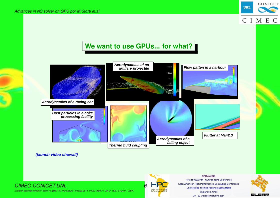
We want to use GPUs... for what?

Aerodynamics of a racing car

Aerodynamics of an artillery projectile Flow patten in a harbour

Dust particles in a coke processing facility

Thermo fluid coupling

Aerodynamics of a falling object

Flutter at Ma=2.3

(launch video showall)


/home/scratch/mstorti/TO-BACKUP/DATA-CD/GPUCONF-VIDEOS/showall.avi


GPUs in HPC

• Some HPC people are skepticalabout the efficient computingpower of GPUs for scientificapplications.• In many works speedup is referred

to available CPU processors, whichis not consistent.• Delivered speedup w.r.t.

mainstream x86 processors isoften much lower than expected.• Strict data parallelism is difficult to

achieve on CFD applications.• Unfortunately, this idea is

reinforced by the fact that GPUscome from the videogame specialeffects industry, not with scientificcomputing.



Solution of incompressible Navier-Stokes flows on GPU

• GPU’s are less efficient for algorithms that require access to the card’s(device) global memory. Shared memory is much faster but usually scarce

(16K per thread block in the Tesla C1060) .• The best algorithms are those that make computations for one cell

requiring only information on that cell and their neighbors. Thesealgorithms are classified as cellular automata (CA).• Lattice-Boltzmann and explicit F?M (FDM/FVM/FEM) fall in this category.• Structured meshes require less data to exchange between cells (e.g.

neighbor indices are computed, no stored), and so, they require lessshared memory. Also, very fast solvers like FFT-based (Fast Fourier

Transform) or Geometric Multigrid are available .



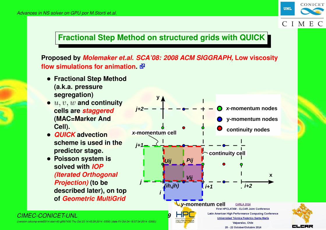
Fractional Step Method on structured grids with QUICK

Proposed by Molemaker et.al. SCA’08: 2008 ACM SIGGRAPH, Low viscosityflow simulations for animation.

• Fractional Step Method(a.k.a. pressuresegregation)• u, v, w and continuity

cells are staggered(MAC=Marker AndCell).• QUICK advection

scheme is used in thepredictor stage.• Poisson system is

solved with IOP(Iterated OrthogonalProjection) (to bedescribed later), on topof Geometric MultiGrid

j

j+1

j+2

i+1 i+2(ih,jh)

Vij

PijUij

x

y

i

y-momentum cell

x-momentum nodes

y-momentum nodes

continuity nodesx-momentum cell

continuity cell


http://portal.acm.org/citation.cfm?id=1632592.1632595


Solution of the Poisson with FFT

• Solution of the Poisson equation is, for large meshes, the more CPUconsuming time stage in Fractional-Step like Navier-Stokes solvers.• We have to solve a linear system Ax = b• The Discrete Fourier Transform (DFT) is an orthogonal transformation

x = Ox = fft(x).• The inverse transformation O−1 = OT is the inverse Fourier Transform

x = OT x = ifft(x).• If the operator matrix A is spatially invariant (i.e. the stencil is the same at

all grid points) and the b.c.’s are periodic, then it can be shown that Odiagonalizes A, i.e. OAO−1 = D.• So in the transformed basis the system of equations is diagonal

(OAO−1) (Ox) = (Ob),

Dx = b,(1)

• For N = 2p the Fast Fourier Transform (FFT) is an algorithm thatcomputes the DFT (and its inverse) in O(N log(N)) operations.



Solution of the Poisson with FFT (cont.)

• So the following algorithm computes the solution of the system inO(N log(N)) ops.

. b = fft(b), (transform r.h.s)

. x = D−1b, (solve diagonal system O(N))

. x = ifft(x), (anti-transform to get the sol. vector)• Total cost: 2 FFT’s, plus one element-by-element vector multiply (the

reciprocals of the values of the diagonal of D are precomputed)• In order to precompute the diagonal values of D,. We take any vector z and compute y = Az,. then transform z = fft(z), y = fft(y),. Djj = yj/zj .



Solution of the Poisson equation on embedded geometries

• FFT solver and GMG are very fast but have several restrictions: invarianceof translation, periodic boundary conditions. They are not well suited forembedded geometries.• One approach for the solution is the IOP (Iterated Orthogonal Projection)

algorithm.• It is based on solving iteratively the Poisson eq. on the whole domain

(fluid+solid). Solving in the whole domain is fast, because algorithms likeGeometric Multigrid or FFT can be used. Also, they are very efficient

running on GPU’s .• However, if we solve in the whole domain, then we can’t enforce the

boundary condition (∂p/∂n) = 0 at the solid boundary which, thenmeans the violation of the condition of impenetrability at the solid

boundary .



The IOP (Iterated Orthogonal Projection) method

The method is based on succesively solve for the incompressibility condition(on the whole domain: solid+fluid), and impose the boundary condition.

on the wholedomain (fluid+solid)

violates impenetrability b.c. satisfies impenetrability b.c.



The IOP (Iterated Orthogonal Projection) method (cont.)

• Fixed point iteration

wk+1 = ΠbdyΠdivwk.

• Projection on the space ofdivergence-free velocity fields:

u′ = Πdiv(u)

u′ = u−∇P,

∆P = ∇ · u,

• Projection on the space of velocityfields that satisfy theimpenetrability boundary condition

u′′ = Πbdy(u′)

u′′ = ubdy, in Ωbdy,

u′′ = u′, in Ωfluid.



Implementation details on the GPU

• We use the CUFFTlibrary.• Per iteration: 2 FFT’s

and Poisson residualevaluation. The FFT onthe GPU Tesla C1060performs at 27 Gflops,(in double precision)where the operationsare counted as5N log2(N).

0

5

10

15

20

25

30

10^3 10^4 10^5 10^6 10^7 10^8

FF

T c

om

pu

tin

g r

ate

[Gfl

op

s]

Vector size



FFT computing rates in GPGPU. GTX-580

0

50

100

150

200

250

105 106 107

FF

T p

roc.

rat

e [G

flo

ps/

sec]

Ncell

64x64x64

128x64x64

128x128x64

128x128x128

256x128x128 256x256x128

double precision

simple precision



FFTW on [email protected] (Sandy Bridge)

0

5000

10000

15000

20000

25000

103 104 105 106 107 108 109

FF

T p

roc.

rat

e [M

flo

ps]

nthreads=1

nthreads=2

nthreads=4

Ncell



NSFVM Computing rates in GPGPU. Scaling

20

40

60

80

100

120

140

160

10-1 100 101 102# of cells [Mcell]

rate

[M

cell/

sec]

GTX-580 SP

GTX-580 DP

C2050-SP

C2050-DP

64x6

4x64

128x

64x6

4

128x

128x

64

128x

128x

128

256x

128x

128

256x

256x

128

256x

256x

256



NSFVM and “Real Time” computing

• For a 128x128x128 mesh (≈ 2Mcell), we have a computing time of2 Mcell/(140 Mcell/sec) = 0.014 secs/time step.• That means 70 steps/sec.• A von Neumann stability analysis shows that the QUICK stabilization

scheme is inconditionally stable if advanced in time with Forward Euler.• With a second order Adams-Bashfort scheme the critical CFL is 0.588.• For NS eqs. the critical CFL has been found to be somewhat lower (≈ 0.5).• If L = 1, u = 1, h = 1/128, ∆t = 0.5h/u = 0.004 [sec], so that we can

compute in 1 sec, 0.28 secs of simulation time. We say ST/RT=0.28.• In the GTX Titan Black we expect to run 3.5x times faster, and has the

double of memory (6 GB versus 3 GB). We expect that it would allow runwith up to 12 Mcells (currently 6 Mcells in the GTX 580).

(launch video nsfvm-bodies-all),


/home/scratch/mstorti/BACKUPED/nsfvm-bodies-all.avi


NSFVM and “Real Time” computing (cont.)



Computing times in GPGPU. Fractional Step components

0

10

20

30

40

50

correctorCG-FFT-solvercomp-divpredictor

tim

e p

arti

cip

atio

n in

to

tal c

om

pu

tin

g t

ime

[%]

128x128x128 mesh

256x256x128 mesh

GTX 580 (Simple precision)



Current work

Current work is done in the following directions

• Improving performance by replacing the QUICK advection scheme byMOC+BFECC (which could be more GPU-friendly).• Implementing a CPU-based renormalization algorithm for free surface

(level-set) flows.• Another important issue is improving the representation (accuracy) of the

solid body surface by using an immersed boundary technique.



Why leave QUICK?

• One of steps of the Fractional Steps Method is the advection step. Wehave to advect the velocity field and we desire a method as less diffusiveas possible, and that allows as large the CFL number as possible.• Also, of course, we want a GPU friendly algorithm.• Previously we used QUICK, but it has a stencil that extends more than one

cell in the upwind direction. This increases shared memory usage anddata transfer. We seek for another low dissipation scheme with a morecompact stencil.



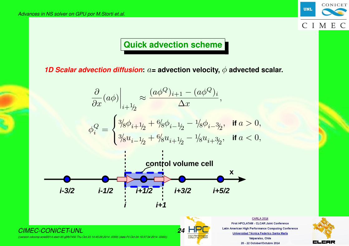
Quick advection scheme

1D Scalar advection diffusion: a= advection velocity, φ advected scalar.

∂

∂x(aφ)

∣∣∣∣i+1/2

≈ (aφQ)i+1 − (aφQ)i∆x

,

φQi =

3/8φi+1/2+ 6/8φi−1/2

− 1/8φi−3/2, if a > 0,

3/8ui−1/2+ 6/8ui+1/2

− 1/8ui+3/2, if a < 0,

x

i+1/2 i+3/2 i+5/2i-1/2i-3/2

control volume cell

i+1i



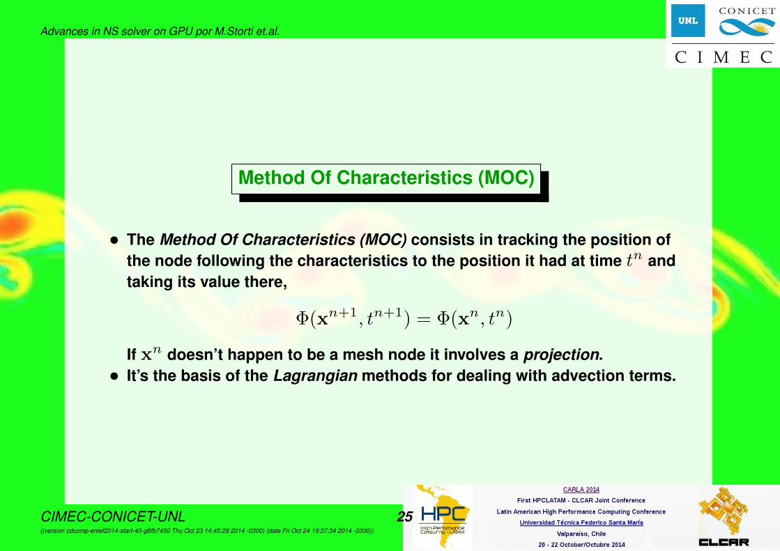
Method Of Characteristics (MOC)

• The Method Of Characteristics (MOC) consists in tracking the position ofthe node following the characteristics to the position it had at time tn andtaking its value there,

Φ(xn+1, tn+1) = Φ(xn, tn)

If xn doesn’t happen to be a mesh node it involves a projection.• It’s the basis of the Lagrangian methods for dealing with advection terms.



Method Of Characteristics (MOC) (cont.)

• So typically MOC has very low diffusion if CFL is an integer number ,

and too diffusive if it is an semi-integer number .• Of course, in the general case (non uniform meshes, non uniform velocity

field) we can’t manage to have an integer CFL number for all the nodes.(launch video video-moc-cfl1), (launch video video-moc-cfl05).

0.2

0.3

0.4

0.5

0.6

0.7

0.8

0.9

1

0 1 2 3 4 5CFL

max(u)

U=1

u(t=0)u(t=10)

L=1periodic

MOC

BFECC+MOC


/home/scratch/mstorti/TO-BACKUP/DATA-CD/GPUCONF-VIDEOS/video-moc-cfl1.avi

/home/scratch/mstorti/TO-BACKUP/DATA-CD/GPUCONF-VIDEOS/video-moc-cfl05.avi


MOC+BFECC

• Assume we have a low order (dissipative) operator (may be SUPG, MOC,or any other) Φt+∆t = L(Φt,u).• The Back and Forth Error Compensation and Correction (BFECC) allows

to eliminate the dissipation error.. Advance forward the state Φt+∆t,∗ = L(Φt,u).. Advance backwards the state Φt,∗ = L(Φt+∆t,∗,−u).

exact w/dissipation error



MOC+BFECC (cont.)

exact w/dissipation error

• If L introduces some dissipative error ε, then Φt,∗ 6= Φt, in factΦt,∗ = Φt + 2ε.• So that we can compensate for the error:

Φt+∆t = L(Φt,∆t)− ε,

= Φt+∆t,∗ − 1/2(Φt,∗ − Φt)

(2)



MOC+BFECC (cont.)

(launch video video-moc-bfecc-cfl05).

0.2

0.3

0.4

0.5

0.6

0.7

0.8

0.9

1

0 1 2 3 4 5CFL

max(u)

U=1

u(t=0)u(t=10)

L=1periodic

MOC

BFECC+MOC


/home/scratch/mstorti/TO-BACKUP/DATA-CD/GPUCONF-VIDEOS/video-moc-bfecc-cfl05.avi


MOC+BFECC (cont.)

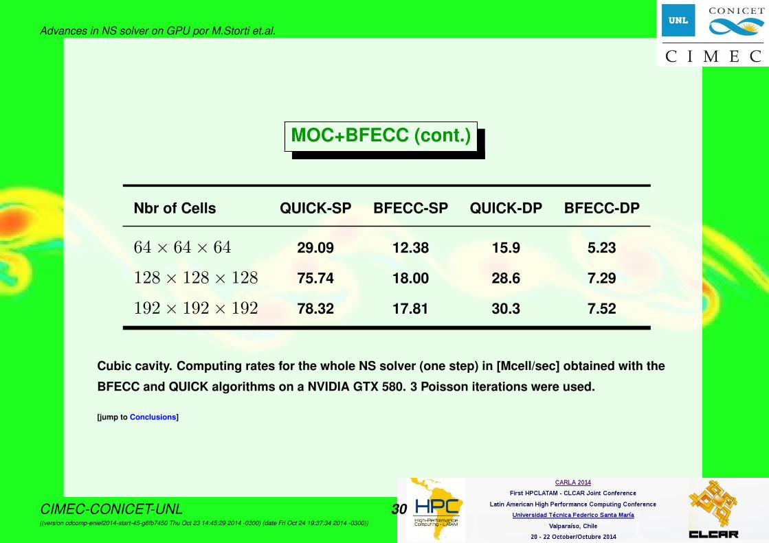
Nbr of Cells QUICK-SP BFECC-SP QUICK-DP BFECC-DP

64× 64× 64 29.09 12.38 15.9 5.23

128× 128× 128 75.74 18.00 28.6 7.29

192× 192× 192 78.32 17.81 30.3 7.52

Cubic cavity. Computing rates for the whole NS solver (one step) in [Mcell/sec] obtained with the

BFECC and QUICK algorithms on a NVIDIA GTX 580. 3 Poisson iterations were used.

[jump to Conclusions]



Analysis of performance

• Regarding the performance results shown above, it can be seen that thecomputing rate of QUICK is at most 4x faster than that of BFECC. SoBFECC is more efficient than QUICK whenever used with CFL > 2, beingthe critical CFL for QUICK 0.5. The CFL used in our simulations is typicallyCFL≈ 5 and, thus, at this CFL the BFECC version runs 2.5 times fasterthan the QUICK version.• The speedup of MOC+BFECC versus QUICK increases with the number of

Poisson iterations. In the limit of very large number of iters (very lowtolerance in the tolerance for Poisson) we expect a speedup 10x (equal tothe CFL ratio).



Validation. Lid driven 3D cubic cavity

• Re=1000, mesh of 128× 128× 128 (2 Mcell). Results compared with Kuet.al (JCP 70(42):439-462 (1987)).• More validation and complete performance study at Costarelli et.al,

Cluster Computing (2013), DOI:10.1007/s10586-013-0329-9.

0 0.2 0.4 0.6 0.8 1−0.4

−0.08

0.24

0.56

0.88

1.2

y

w(y

)

−0.5 −0.34 −0.18 −0.02 0.14 0.3

0

0.2

0.4

0.6

0.8

1

v(z)

z

Ku et al.NSFDM



Renormalization

Even with a high precision, low dissipative algorithm for transporting the levelset function Φ we have to renormalize Φ→ Φ′ with a certain frequency thelevel set function.

• Requirements on the renormalizationalgorithm are:. Φ′ must preserve as much as posible

the 0 level set function (interface) Γ.. Φ′ must be as regular as possible near

the interface.. Φ′ must have a high slope near the

interface.. Usually the signed distance function is

used, i.e.

Φ′(x) = sign(Φ(x)) miny∈Γ||y − x|| xΦ

Γ

Φ (renormalized)

Γ Γ



Renormalization (cont.)

• Computing plainly the distancefunction is O(NNΓ) where NΓ is thenumber of points on the interface. Thisscales typically∝ N1+(nd−1)/nd

(N5/3 in 3D).

• Many variants are based in solving theEikonal equation

|∇Φ| = 1,

• As it is an hyperbolic equation it canbe solved by a marching technique.The algorithm traverses the domainwith an advancing front starting fromthe level set.• However, it can develop caustics

(shocks), and rarefaction waves. So,an entropy condition must be enforced.

caustic

expansion fan



Renormalization (cont.)

• The Fast Marching algorithmproposed by Sethian (Proc NatAcad Sci 93(4):1591-1595 (1996)) ,is a fast (near optimal) algorithmbased on Dijkstra’s algorithm forcomputing minimum distances ingraphs from a source set. (Note:the original Dijkstra’s algorithm isO(N2), not fast. The fast versionusing a priority queue is due toFredman and Tarjan (ACM Journal24(3):596-615, 1987), and thecomplexity isO(N log(|Q|)) ∼ O(N log(N))).

Q=advancing front F=far-away

Level set


http://www.pnas.org/content/93/4/1591.short

http://www.pnas.org/content/93/4/1591.short

http://dx.doi.org/10.1145/28869.28874

http://dx.doi.org/10.1145/28869.28874


The Fast Marching algorithm

• We explain for the positive part Φ > 0.Then the algorithm is reversed for Φ < 0.• All nodes are in either: Q=advancing front,F=far-away , I=frozen/inactive. Theadvancing front sweeps the domainstarting at the level set and converts Fnodes to I .• Initially Q = nodes that are in contact

with the level set. Their distance to theinterface is computed for each cut-cell.The rest is in F =far-away.• loop: Take the node X in Q closest to the

interface. Move it from Q→ I .• Update all distances from neighbors to X

and move them from F → Q.• Go to loop.• Algorithm ends when Q = ∅. Q=advancing front F=far-away

Level set

I= frozen/inactive

X



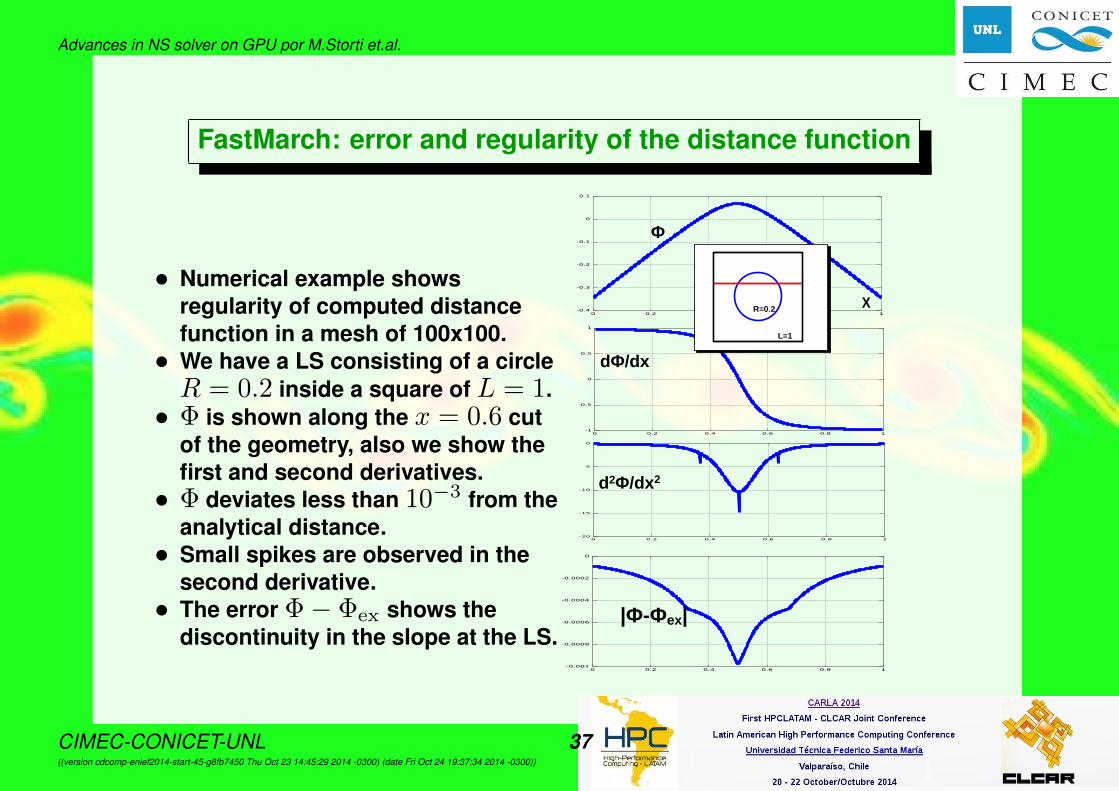
FastMarch: error and regularity of the distance function

• Numerical example showsregularity of computed distancefunction in a mesh of 100x100.• We have a LS consisting of a circleR = 0.2 inside a square of L = 1.• Φ is shown along the x = 0.6 cut

of the geometry, also we show thefirst and second derivatives.• Φ deviates less than 10−3 from the

analytical distance.• Small spikes are observed in the

second derivative.• The error Φ− Φex shows the

discontinuity in the slope at the LS.

-0.4

-0.3

-0.2

-0.1

0

0.1

0 0.2 0.4 0.6 0.8 1

X

-1

-0.5

0

0.5

1

0 0.2 0.4 0.6 0.8 1

dΦ/dx

-20

-15

-10

-5

0

0 0.2 0.4 0.6 0.8 1

d2Φ/dx2

-0.001

-0.0008

-0.0006

-0.0004

-0.0002

0

0 0.2 0.4 0.6 0.8 1

|Φ-Φex|

L=1

R=0.2

Φ



FastMarch: implementation details

• Complexity is O(N)× the cost of finding the node in Q closest to thelevel set.• This can be implemented in a very efficient way with a priority queue

implemented in top of a heap. In this way finding the closest node isO(log |Q|). So the total cost is

O(N log |Q|) ≤ O(N log(N(nd−1)/nd)) = O(N logN

2/3) (in 3D).• The standard C++ class priority_queue<> is not appropriate

because don’t give access to the elements in the queue.• We implemented the heap structure on top of a vector<> and anunordered_map<> (hash-table based) that tracks the Q-nodes in thestructure. The hash function used is very simple.



FastMarch renorm: Efficiency

• The Fast Marching algorithm isO(N log |Q|) where N is thenumber of cells and |Q| the size ofthe advancing front.• Rates were evaluated in an Intel

[email protected] (Nehalem).• Computing rate is practically

constant and even decreases withhigh N .• Since the rate for the NS-FVM

algorithm is >100 [Mcell/s],renormalization at a frequencygreater than 1/200 steps would betoo expensive.• Cost of renormalization step is

reduced with band renormalizationand parallelism (SMP).

N (Nbr of cells per side)

pro

cess

ing

rat

e [M

cells

/s]

2048

x204

8

1024

x102

4

512x

512

256x

256

128x

128

64x6

4

32x3

2

0

0.1

0.2

0.3

0.4

0.5

0.6

103 104 105 106 107



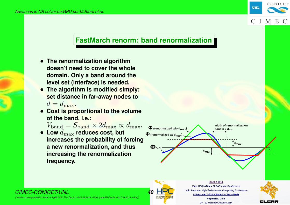
FastMarch renorm: band renormalization

• The renormalization algorithmdoesn’t need to cover the wholedomain. Only a band around thelevel set (interface) is needed.• The algorithm is modified simply:

set distance in far-away nodes tod = dmax.• Cost is proportional to the volume

of the band, i.e.:Vband = Sband × 2dmax ∝ dmax.• Low dmax reduces cost, but

increases the probability of forcinga new renormalization, and thusincreasing the renormalizationfrequency.

xΦold

Φ (renormalized w/o dmax)

dmax

dmax

Φ (renormalized w/ dmax)

width of renormalization band = 2 dmax



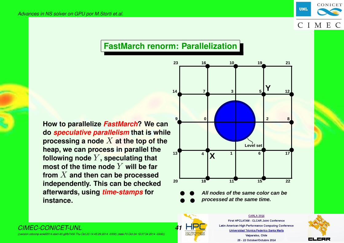
FastMarch renorm: Parallelization

How to parallelize FastMarch? We cando speculative parallelism that is whileprocessing a node X at the top of theheap, we can process in parallel thefollowing node Y , speculating thatmost of the time node Y will be farfrom X and then can be processedindependently. This can be checkedafterwards, using time-stamps forinstance.

Level set

0

1

2

3

4 6

57

8

17

2215111820

13

9

14

23 16 10 19 21

12

All nodes of the same color can beprocessed at the same time.

X

Y



FastMarch renorm: Parallelization (cont.)

• How much nodes can beprocessed concurrently? Itturns out that thesimultaneity (number ofnodes that can beprocessed simultaneously)grows linearly withrefinement.• Average simultaneity is

16x16: 11.35832x32: 20.507• Percentage of times

simultaneity is≥4:16x16: 93.0%32x32: 98.0%

0

10

20

30

40

50

60

70

80

0 0.2 0.4 0.6 0.8 1

nu

mer

of

ind

ep

en

den

t p

oin

ts

% advance front

0

10

20

30

40

50

60

70

80

0 0.2 0.4 0.6 0.8 1% front nodes

nu

mer

of

ind

ep

en

den

t p

oin

ts



FastMarching: computational budget

• With band renormalization and SMP parallelization we expect a rate of20 Mcell/s.• That means that a 1283 mesh (2 Mcell) can be done in 100 ms.• This is 7x times the time required for one time step (14 ms).• Renormalization will be amortized if the renormalization frequency is more

than 1/20 time steps.• Transfer of the data to and from the processor through the PCI Express 2.0

x 16 channel (∼4 GB/s transfer rate) is in the order of 10 ms.• BTW: note that transfers from the CPU to/from the card are amortized if

they are performed each 1:10 steps or so. Such transfers can’t be done alltime steps.



Fluid structure interaction

• In the previous examples we have shown several cases of rigid solidbodies moving immersed in a fluid. In those cases the position of thebody is prescribed beforehand.• A more complex case is when the position of the body results from the

interaction with the fluid.• In general if the body is not rigid we have to solve the elasticity equations

in the body Ωbdy(t). We assume here that the body is rigid, so that wejust solve for the 6 d.o.f. of the rigid with the linear and angularmomentum of the body.



Fluid structure in the real world

Three Gorges (PR China) dam Francis Turbine

Belomone Francis Turbineinstallation

Sayano–Shushenskaya (Russia) DamMachine room prior to 2009 accident

Sayano–Shushenskaya (Russia) DamMachine room after 2009 accident

• IMPSA (Industria Metalurgica Pescarmona) is manufacturing three Francisturbines for the Belo Monte (Brazil) dam. Once in operation it would be the3rd largest dam in the world.• Ignition of a rocket engine (launch video video-simulacion-motor-cohete).


/home/scratch/mstorti/TO-BACKUP/DATA-CD/GPUCONF-VIDEOS/video-simulacion-motor-cohete.avi


Fluid structure in the real world (cont.)

• CIMEC computed the rotordynamiccoefficients, that is a reduced parameterrepresentation of the fluid in the gapbetween stator and rotor. (launch video

movecyl-tadpoles)

• The rotordynamic coefficientes representthe forces of the fluid on to the rotor as therotor orbits around its centered position.They are used as a component of thedesign of the structural part of the turbine.• They represent the added mass, damping,

and stiffness (a.k.a. Lomakin effect).• The geometry is very complex: a circular

corona of diameter 8m, gap 3mm, andheight 2m.


/home/scratch/mstorti/TO-BACKUP/DATA-CD/GPUCONF-VIDEOS/movecyl-tadpoles.avi

/home/scratch/mstorti/TO-BACKUP/DATA-CD/GPUCONF-VIDEOS/movecyl-tadpoles.avi


A buoyant fully submerged sphere

• Fluid is water ρfluid = 1000 [kg/m3].• The body is a smooth sphere D =10cm, fully

submerged in a box of L =39cm. Soliddensity is ρbdy = 366 [kg/m3] ≈ 0.4 ρfluid

so the body has positive buoyancy. The buoy(sphere) is tied by a string to an anchor pointat the center of the bottom side of the box.• Ths box is subject to horizontal harmonic

oscillations

xbox = Abox sin(ωt),



Spring-mass-damper oscillator

• The acceleration of the box creates a driving force on the sphere. Notethat as the sphere is positively buoyant the driving force is in phase withthe displacement. That means that if the box accelerates to the right, thenthe sphere tends to move in the same direction. (launch video p2-f09)

• The buoyancy of the sphere produces a restoring force that tends to keepaligned the string with the vertical direction.• The mass of the sphere plus the added mass of the liquid gives inertia.• The drag of the fluid gives a damping effect.• So the system can be approximated as a (nonlinear) spring-mass-damper

oscillator

inertia︷︸︸︷mtotx+

damp︷︸︸︷0.5ρflCdA|v|x+

spring︷︸︸︷(mflotg/L)x =

driving frc︷︸︸︷mflotabox,

mtot = mbdy +madd, mflot = md −mbdy,

madd = Cmaddmd, Cmadd ≈ 0.5, md = ρflVbdy


/home/scratch/mstorti/TO-BACKUP/DATA-CD/GPUCONF-VIDEOS/p2-f09.avi


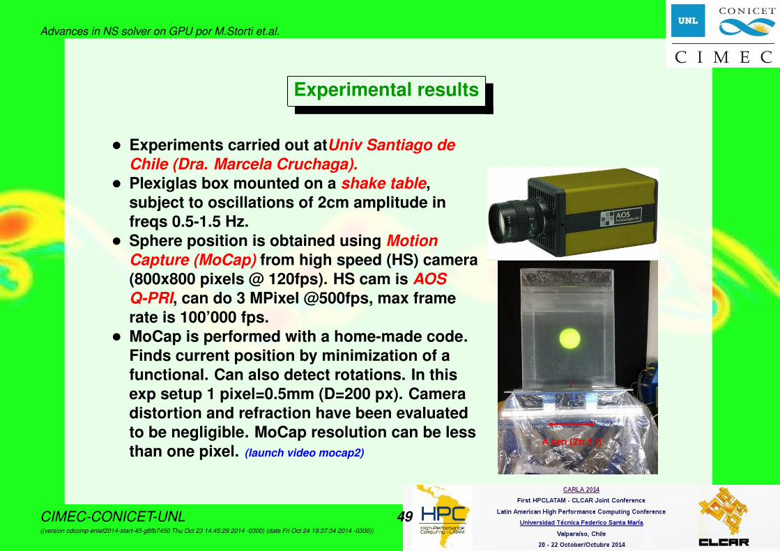
Experimental results

• Experiments carried out atUniv Santiago deChile (Dra. Marcela Cruchaga).• Plexiglas box mounted on a shake table,

subject to oscillations of 2cm amplitude infreqs 0.5-1.5 Hz.• Sphere position is obtained using Motion

Capture (MoCap) from high speed (HS) camera(800x800 pixels @ 120fps). HS cam is AOSQ-PRI, can do 3 MPixel @500fps, max framerate is 100’000 fps.• MoCap is performed with a home-made code.

Finds current position by minimization of afunctional. Can also detect rotations. In thisexp setup 1 pixel=0.5mm (D=200 px). Cameradistortion and refraction have been evaluatedto be negligible. MoCap resolution can be lessthan one pixel. (launch video mocap2)


/home/scratch/mstorti/TO-BACKUP/DATA-CD/GPUCONF-VIDEOS/mocap2.avi


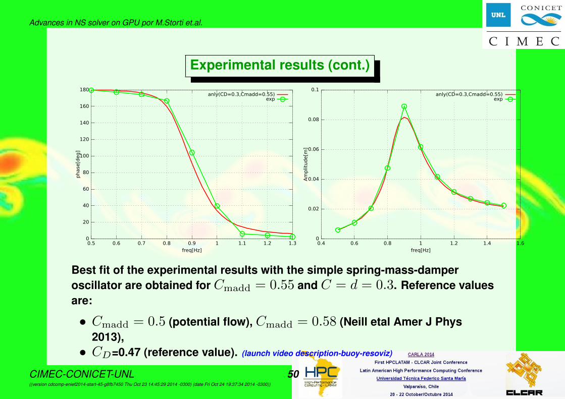
Experimental results (cont.)

0

20

40

60

80

100

120

140

160

180

0.5 0.6 0.7 0.8 0.9 1 1.1 1.2 1.3

phase[deg]

freq[Hz]

anly(CD=0.3,Cmadd=0.55)exp

0

0.02

0.04

0.06

0.08

0.1

0.4 0.6 0.8 1 1.2 1.4 1.6

Amplitude[m

]

freq[Hz]

anly(CD=0.3,Cmadd=0.55)exp

Best fit of the experimental results with the simple spring-mass-damperoscillator are obtained for Cmadd = 0.55 and C = d = 0.3. Reference valuesare:

• Cmadd = 0.5 (potential flow), Cmadd = 0.58 (Neill etal Amer J Phys2013),• CD=0.47 (reference value). (launch video description-buoy-resoviz)


/home/scratch/mstorti/TO-BACKUP/DATA-CD/GPUCONF-VIDEOS/description-buoy-resoviz.avi


Computational FSI model

• The fluid structure interaction is performed with a partitioned FluidStructure Interaction (FSI) technique.• Fluid is solved in step [tn, tn+1 = tn + ∆t] between the known position

xn of the body at tn and an extrapolated (predicted) position xn+1,P attn+1.• Then fluid forces (pressure and viscous tractions) are computed and the

rigid body equations are solved to compute the true position of the solidxn+1.• The scheme is second order precision. It can be put as a fixed point

iteration and iterated to convergence (enhancing stability).• The rigid body eqs. are now:

mbdyx+ (mflotg/L)x = Ffluid +mflotabox

where Ffluid = Fdrag + Fadd are now computed with the CFD-NS-FVMcode.



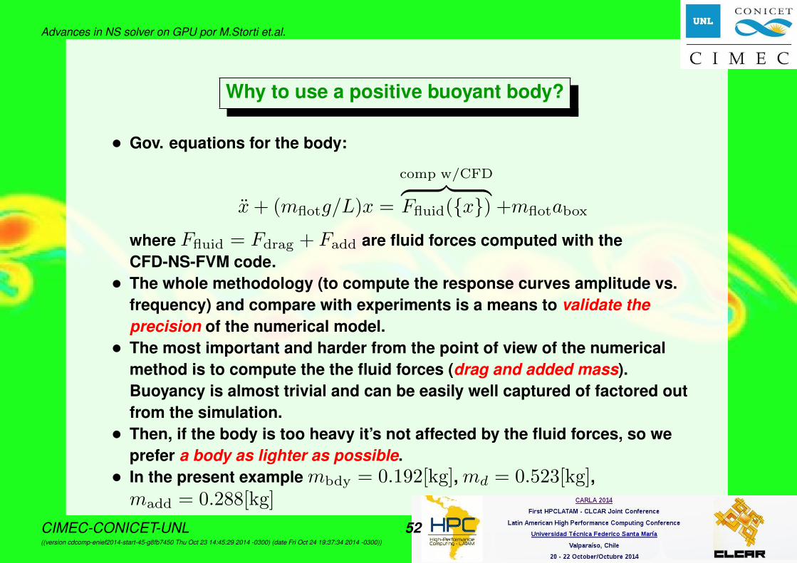
Why to use a positive buoyant body?

• Gov. equations for the body:

x+ (mflotg/L)x =

comp w/CFD︷︸︸︷Ffluid(x) +mflotabox

where Ffluid = Fdrag + Fadd are fluid forces computed with theCFD-NS-FVM code.• The whole methodology (to compute the response curves amplitude vs.

frequency) and compare with experiments is a means to validate theprecision of the numerical model.• The most important and harder from the point of view of the numerical

method is to compute the the fluid forces (drag and added mass).Buoyancy is almost trivial and can be easily well captured of factored outfrom the simulation.• Then, if the body is too heavy it’s not affected by the fluid forces, so we

prefer a body as lighter as possible.• In the present example mbdy = 0.192[kg], md = 0.523[kg],madd = 0.288[kg]



Numerical results

• Results with NS-VFM-GPGPU on GTX-580 3GB RAM. 6 Mcells. Rate 140Mcell/sec. (launch video fsi-boya-gpu-vorticity), (launch video gpu-corte), (launch video

particles-buoyp5)

• Also as a reference PETSc-FEM results included. Boundary fitted mesh400 k-elements. (launch video fem-mesh-quality)

Vorticity isosurface

velocity at sym plane

tadpoles

FEM mesh distortion


/home/scratch/mstorti/TO-BACKUP/DATA-CD/GPUCONF-VIDEOS/fsi-boya-gpu-vorticity.avi

/home/scratch/mstorti/TO-BACKUP/DATA-CD/GPUCONF-VIDEOS/gpu-corte.avi

/home/scratch/mstorti/TO-BACKUP/DATA-CD/GPUCONF-VIDEOS/particles-buoyp5.avi

/home/scratch/mstorti/TO-BACKUP/DATA-CD/GPUCONF-VIDEOS/particles-buoyp5.avi

/home/scratch/mstorti/TO-BACKUP/DATA-CD/GPUCONF-VIDEOS/fem-mesh-quality.avi


Comparison of experimental and numerical results

0

0.02

0.04

0.06

0.08

0.1

0.5 0.6 0.7 0.8 0.9 1 1.1 1.2 1.3

Amplitude[m

]

freq[Hz]

expanal(CD=0.3,Cmadd=0.55)

NSFVM/GPUFEM

-200

-150

-100

-50

0

0.5 0.6 0.7 0.8 0.9 1 1.1 1.2 1.3Phase[deg]

freq[Hz]

expanal(CD=0.3,Cmadd=0.55)

NSFVM/GPUFEM



Conclusions

• The NS-FVM implementation reaches high computing rates in GPGPUhardware (O(140 Mcell/s)).• It can represent complex moving bodies without meshing.• Surface representation of bodies can be made second order (not

implemented yet).• Solution of the Poisson problem is currently a significant part of the

computing time. This is reduced by using the AGP preconditioner andMOC-BFECC combination.• MOC+BFECC has lower computing rates than QUICK (4x slower) but may

reach CFL=5 (versus CFL=0.5 for QUICK). So we get a speedup of 2.5x.• Speedups may be higher if lower tolerances are required for the Poisson

stage (more Poisson iters).• Fluid-Structure interaction is solved with a partitioned strategy and is

validated against experimental and numerical (FEM) results.



Acknowledgments

This work has received financial support from

• Consejo Nacional de Investigaciones Cientıficas y Tecnicas (CONICET,Argentina, PIP 5271/05),• Universidad Nacional del Litoral (UNL, Argentina, grant CAI+D

2009-65/334),• Agencia Nacional de Promocion Cientıfica y Tecnologica (ANPCyT,

Argentina, grants PICT-1506/2006, PICT-1141/2007, PICT-0270/2008), and• European Research Council (ERC) Advanced Grant, Real Time

Computational Mechanics Techniques for Multi-Fluid Problems(REALTIME, Reference: ERC-2009-AdG, Dir: Dr. Sergio Idelsohn).

The authors made extensive use of Free Software as GNU/Linux OS, GCC/G++compilers, Octave, and Open Source software as VTK among many others. Inaddition, many ideas from these packages have been inspiring to them.


http://www.conicet.gov.ar

http://www.unl.edu.ar

http://www.agencia.gov.ar

http://erc.europa.eu

http://erc.europa.eu/index.cfm?fuseaction=page.display&topicID=518

http://erc.europa.eu/index.cfm?fuseaction=page.display&topicID=518

http://www.gnu.org