HAL Id: hal-00664777https://hal.inria.fr/hal-00664777

Submitted on 31 Jan 2012

HAL is a multi-disciplinary open accessarchive for the deposit and dissemination of sci-entific research documents, whether they are pub-lished or not. The documents may come fromteaching and research institutions in France orabroad, or from public or private research centers.

L’archive ouverte pluridisciplinaire HAL, estdestinée au dépôt et à la diffusion de documentsscientifiques de niveau recherche, publiés ou non,émanant des établissements d’enseignement et derecherche français ou étrangers, des laboratoirespublics ou privés.

Advances in Probabilistic Model CheckingMarta Kwiatkowska, David Parker

To cite this version:Marta Kwiatkowska, David Parker. Advances in Probabilistic Model Checking. O. Grumberg andT. Nipkow and J. Esparza. Proc. 2011 Marktoberdorf Summer School: Tools for Analysis andVerification of Software Safety and Security, IOS Press, 2012. <hal-00664777>

Advances in Probabilistic Model Checking

Marta KWIATKOWSKA a, David PARKER a

a Department of Computer Science, University of Oxford, Oxford, UK

Abstract. Probabilistic model checking is an automated verification

method that aims to establish the correctness of probabilistic systems.Probability may arise, for example, due to failures of unreliable compo-

nents, communication across lossy media, or through the use of randomi-

sation in distributed protocols. Probabilistic model checking enables arange of exhaustive, quantitative analyses of properties such as “the

probability of a message being delivered within 5ms is at least 0.89”.

In the last ten years, probabilistic model checking has been success-fully applied to numerous real-world case studies, and is now a highly

active field of research. This tutorial gives an introduction to proba-bilistic model checking, as well as presenting material on selected recent

advances. The first half of the tutorial concerns two classical probabilis-

tic models, discrete-time Markov chains and Markov decision processes,explaining the underlying theory and model checking algorithms for the

temporal logic PCTL. The second half discusses two advanced topics:

quantitative abstraction refinement and model checking for probabilis-tic timed automata. We also briefly summarise the functionality of the

probabilistic model checker PRISM, the leading tool in the area.

Keywords. Markov models; Probabilistic temporal logics; Probabilistic

model checking; Quantitative model checking

1. Introduction

Probabilistic modelling is widely used for the design and analysis of computersystems. Probability is typically employed to quantify unreliable or unpredictablebehaviour, for example in fault-tolerant systems and communication protocols,where properties such as component failure and message loss can be expressedprobabilistically. In distributed co-ordination algorithms, randomness serves as asymmetry breaker in order to derive efficient algorithms, see e.g. random back-off schemes in IEEE 802.11 or Bluetooth device discovery, and population proto-cols [4]. Traditionally, probability has also been used as a tool to analyse systemperformance and Quality of Service.

Probabilistic model checking is an automatic procedure for establishing if adesired property holds in a probabilistic system model. Conventional model check-ers input a description of a model, representing a state-transition system, anda specification, typically a formula in some temporal logic, and return “yes” or“no”, indicating whether or not the model satisfies the specification. In the lattercase, a diagnostic trace, referred to as a counterexample, is returned. In proba-bilistic model checking, the models are probabilistic (typically variants of Markov

1

chains), in the sense that they encode the probability of making a transition be-tween states instead of simply the existence of such a transition. A probabilityspace induced on the executions of the system enables calculation of the likelihoodof the occurrence of certain events of interest. This in turn allows quantitativestatements to be made about the system’s behaviour, expressed as probabilitiesor expectations, in addition to the qualitative statements made by conventionalmodel checking. Probabilities are captured via probabilistic operators that extendconventional (timed or untimed) temporal logics. Models can be additionally an-notated with costs and rewards, and the reward operator enables the computationof expectations with respect to the underlying probability space. The extendedlogics can express the following probabilistic and reward specifications:

• for a randomised leader election algorithm: “leader election is eventuallyresolved with probability 1”;

• for a security protocol: “the chance of intrusion is at most 0.0001%”;• for a web service: “what is the probability of a response within 5ms?”;• for a wireless communication protocol: “what is the worst-case expected

time for delivering a data packet?”;• for a battery-powered device: “the maximum expected energy consumption

in 24hrs is at most 190J”.

Note that answers to the above queries can be truth values, when the specificationsimply asks for a comparison to a probability threshold, or quantitative, returningthe actual probability or expectation.

The first algorithms for probabilistic model checking were proposed in the1980s [36,63,21], originally focussing on qualitative probabilistic temporal prop-erties (i.e. those satisfied with probability 1 or 0) but later also introducing quan-titative properties. These were followed by various extensions [35,14,8] and firstimplementations [34,5]. However, the first industrial strength probabilistic modelcheckers were developed only in the 2000s [24,40], when the field matured. Prob-abilistic model checking draws on conventional model checking, since it relies onreachability analysis of the underlying transition system, and to this end tech-niques such as symbolic model checking, symmetry reduction, counterexamplesand abstraction refinement have been usefully adapted. This is combined withappropriate numerical methods, such as linear algebra or linear programming, inorder to provide the calculation of the actual likelihoods and expectations. Themain advantage is that the analysis is exhaustive, resulting in numerically exactanswers to the temporal logic queries (in contrast to approximate analysis meth-ods such as simulation), and is able to express detailed temporal constraints onthe system’s executions (in contrast to analytical methods).

Probabilistic model checking has been successfully applied in a multitude ofdomains: distributed coordination algorithms, wireless communication protocols,security, anonymity and quantum cryptographic protocols, nanotechnology de-signs, power management and modelling of biological processes. Several flaws andunusual features have been discovered using the techniques; for more information,see e.g. [50,67]. As more real-world case studies are being analysed, user expecta-tions are growing with regards to the efficiency and accuracy of the results, the de-gree of automation of the methods, and the range of systems that can be modelled

2

and analysed. Probabilistic model checking has developed into an exciting andhighly active field of research that covers the full spectrum, from theory, throughimplementation techniques, to applications, and we are pleased to introduce thereader to the main concepts, as well describe some research highlights.

Outline. This tutorial begins with an introduction to probabilistic modelchecking based on two classical probabilistic models with discrete states and dis-crete probability distributions – discrete time Markov chains and Markov decisionprocesses – which respectively model fully probabilistic systems and concurrentprobabilistic systems. We introduce the probabilistic temporal logic PCTL and itsreward extension, which is interpreted over states of the two classical models, andexplain the corresponding model checking methods. The second half of the tutorialdiscusses two advanced topics: quantitative abstraction refinement for Markov de-cision processes and model checking for probabilistic timed automata. The lattercan be viewed as Markov decision processes extended with real-valued clocks, andthe former method underpins their model checking, in addition to model check-ing for real probabilistic software. The models, specification formalisms and tech-niques introduced here are supported by the probabilistic model checker PRISM[55,67], which is also briefly described.

2. Preliminaries

Let Ω be a sample set, the set of possible outcomes of an experiment. A pair(Ω,F) is said to be a sample space if F is a σ-field of subsets of Ω, often builtfrom basic cylinders/cones by closing w.r.t. countable unions and complement.The elements of F are called events. A triple (Ω,F , µ) is a probability space ifµ is a probability measure over F , i.e. 0 6 µ(A) 6 1 for all A ∈ F ; µ(∅) = 0,µ(Ω) = 1 and µ(

⋃∞k=1Ak) =

∑∞k=1 µ(Ak) for disjoint Ak.

Let (Ω,F , µ) be a probability space. A measurable function X : Ω → R>0

is said to be a random variable. The expectation (or average value) of X withrespect to the measure µ is given by the following integral:

E[X]def=

∫ω∈Ω

X(ω) dµ .

For a countable set S, a discrete probability distribution on S is a function µ :S → [0, 1] such that

∑s∈S µ(s) = 1. The set of all probability distributions over

the S is denoted Dist(S).

3. Model Checking for Discrete-time Markov Chains

We begin with the simplest probabilistic model, that of discrete-time Markovchains (DTMCs), which model systems whose behaviour at each point in timecan be described by a discrete probabilistic choice over several possible outcomes.This might represent, for example, an electronic coin toss, as used to implementa randomised algorithm, or transmission of a message over an unreliable channel,

3

a

b 0.4 0.1

0.6

1 0.3

0.7 0.1

0.3

0.9 1 0.1

0.5

s1 s3 s5

s0 s2 s4

P =

0 0.1 0.9 0 0 0

0.4 0 0 0.6 0 0

0 0 0.1 0.1 0.5 0.3

0 0 0 1 0 0

0 0 0 0 1 0

0 0 0 0 0.7 0.3

Figure 1. An example DTMC and its transition probability matrix P.

which is known to fail with a certain probability. Essentially, a DTMC can bethought of as a labelled state-transition system in which each transition is anno-tated with a probability value indicating the likelihood of its occurrence. For thismodel, we introduce PCTL, a probabilistic and reward extension of the branchingtime logic CTL, and briefly describe the underlying algorithms.

3.1. Discrete-time Markov Chains

A discrete time Markov chain consists of discrete states, representing the con-figurations of the system, and has transitions governed by (discrete) probabilitydistributions over the target states.

Definition 1 (Discrete-time Markov chain) A discrete-time Markov chain (DTMC)is a tuple D = (S, s,P, L) where S is a (countable) set of states, s ∈ S isan initial state, P : S×S → [0, 1] is a transition probability matrix such that∑s′∈S P(s, s′) = 1 for all s ∈ S, and L : S → 2AP is a labelling function mapping

each state to a set of atomic propositions taken from a set AP.

Each element P(s, s′) of the matrix P gives the probability of taking a transitionfrom s to s′, where the transition is assumed to take a discrete time-step. Thismeans that there is no notion of real time, though reasoning about discrete timeis possible through state variables keeping track of time and ‘counting’ transitionsteps. Note that there are no deadlocks, and all terminating states are modelledwith a self-loop.

We can unfold a DTMC model into a set of paths. A path through aDTMC is a non-empty (finite or infinite) sequence of states ω = s0 s1 s2 . . . withP(si, si+1) > 0 for all i > 0. The probability matrix P induces a probability spaceon the set of infinite paths Paths, which start in the state s, using the cylinderconstruction [48] as follows. An observation of a finite path determines a basicevent (cylinder). Let s = s0. For π = s0s1 . . . sn, we define the probability mea-sure Prfin

s for the π-cylinder by putting Prfins = 1 if π consists of a single state,

and Prfins = P(s0, s1) ·P(s1, s2) · . . . ·P(sn−1, sn) otherwise. This extends to a

unique measure Prs on the set of infinite paths Paths [48].

Example 1 Figure 1 shows an example of a DTMC D = (S, s,P, L) with 6 statesS = s0, . . . , s5 and initial state s = s0. The transition probability matrix P isalso shown in Figure 1. The set of atomic propositions AP is a, b and functionL labels s1 with a and s4 with b.

4

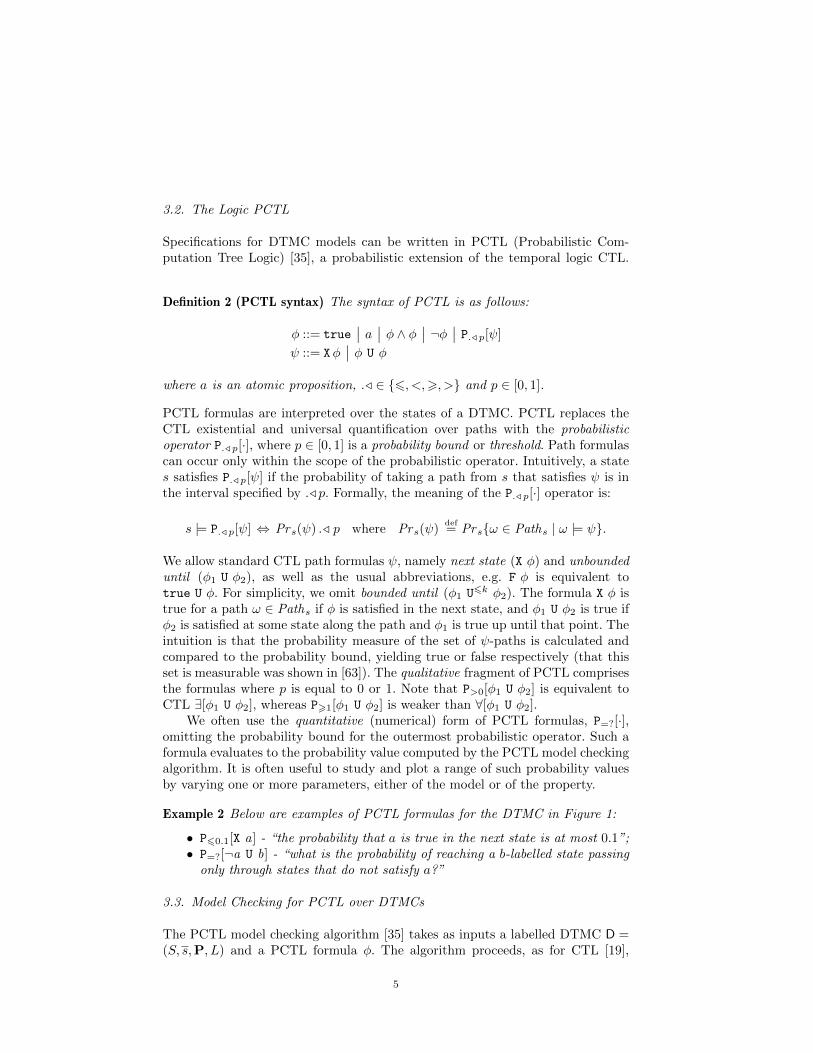
3.2. The Logic PCTL

Specifications for DTMC models can be written in PCTL (Probabilistic Com-putation Tree Logic) [35], a probabilistic extension of the temporal logic CTL.

Definition 2 (PCTL syntax) The syntax of PCTL is as follows:

φ ::= true∣∣ a ∣∣ φ ∧ φ ∣∣ ¬φ ∣∣ P./ p[ψ]

ψ ::= Xφ∣∣ φ U φ

where a is an atomic proposition, ./ ∈ 6, <,>, > and p ∈ [0, 1].

PCTL formulas are interpreted over the states of a DTMC. PCTL replaces theCTL existential and universal quantification over paths with the probabilisticoperator P./ p[·], where p ∈ [0, 1] is a probability bound or threshold. Path formulascan occur only within the scope of the probabilistic operator. Intuitively, a states satisfies P./ p[ψ] if the probability of taking a path from s that satisfies ψ is inthe interval specified by ./ p. Formally, the meaning of the P./ p[·] operator is:

s |= P./ p[ψ] ⇔ Prs(ψ) ./ p where Prs(ψ)def= Prsω ∈ Paths | ω |= ψ.

We allow standard CTL path formulas ψ, namely next state (X φ) and unboundeduntil (φ1 U φ2), as well as the usual abbreviations, e.g. F φ is equivalent totrue U φ. For simplicity, we omit bounded until (φ1 U6k φ2). The formula X φ istrue for a path ω ∈ Paths if φ is satisfied in the next state, and φ1 U φ2 is true ifφ2 is satisfied at some state along the path and φ1 is true up until that point. Theintuition is that the probability measure of the set of ψ-paths is calculated andcompared to the probability bound, yielding true or false respectively (that thisset is measurable was shown in [63]). The qualitative fragment of PCTL comprisesthe formulas where p is equal to 0 or 1. Note that P>0[φ1 U φ2] is equivalent toCTL ∃[φ1 U φ2], whereas P>1[φ1 U φ2] is weaker than ∀[φ1 U φ2].

We often use the quantitative (numerical) form of PCTL formulas, P=?[·],omitting the probability bound for the outermost probabilistic operator. Such aformula evaluates to the probability value computed by the PCTL model checkingalgorithm. It is often useful to study and plot a range of such probability valuesby varying one or more parameters, either of the model or of the property.

Example 2 Below are examples of PCTL formulas for the DTMC in Figure 1:

• P60.1[X a] - “the probability that a is true in the next state is at most 0.1”;• P=?[¬a U b] - “what is the probability of reaching a b-labelled state passing

only through states that do not satisfy a?”

3.3. Model Checking for PCTL over DTMCs

The PCTL model checking algorithm [35] takes as inputs a labelled DTMC D =(S, s,P, L) and a PCTL formula φ. The algorithm proceeds, as for CTL [19],

5

by bottom-up traversal of the parse tree for φ, recursively computing the set

Sat(φ′) = s ∈ S | s |=φ′ of states satisfying each subformula φ′. Therefore, the

algorithm will eventually compute the set of all states satisfying φ. To establish if

a given state s satisfies φ, we simply check if s ∈ Sat(φ). For the non-probabilistic

operators, the algorithm computes as for CTL:

Sat(true) = SSat(a) = s ∈ S | a ∈ L(s)

Sat(¬φ) = S \ Sat(φ)Sat(φ1 ∧ φ2) = Sat(φ1) ∩ Sat(φ2) .

For the probabilistic operator P./p[ψ], we have:

Sat(P./p[ψ]) = s ∈ S | Prs(ψ) ./ p .

It is convenient to view the DTMC as the matrix P and Sat(φ) as a column

vector φ : S −→ 0, 1 given by φ(s) = 1 if s |= φ and 0 otherwise. Consider the

next state operator. The probabilities for all states can then be computed by a

single matrix-by-vector multiplication, written in vector notation Pr(Xφ) = P ·φ.

For the path formula φ1 U φ2, the probabilities Prs(φ1 U φ2) are obtained as

the unique solution of the linear equation system in variables xs | s ∈ S:

xs =

0 if s ∈ Sno

1 if s ∈ Syes∑s′∈S P(s, s′) · xs′ if s ∈ S?

where Sno def= Sat(P6 0[φ1 U φ2]) and Syes def

= Sat(P> 1[φ1 U φ2]) denote the sets

of all states that satisfy φ1 U φ2 with probability exactly 0 and 1, respectively,

and S? = S \ (Sno ∪ Syes).

The sets Sno and Syes are precomputed using conventional fixed point com-

putations. For example, for Sno , we first compute the set of states from which we

can reach, with positive probability, a φ2-state passing only through states satis-

fying φ1, and then subtract this set from S. Since the values for the precomputed

states are known (0 or 1), the solution of the resulting linear equation system in

|S?| variables can be obtained by any direct method (e.g. Gaussian elimination)

or iterative method (e.g. Jacobi, Gauss-Seidel). For qualitative PCTL properties,

it suffices to use these precomputation algorithms alone. Note that the precompu-

tation algorithms determine the exact probability in case it is 0 or 1, thus avoiding

the problem of round-off errors that are typical for numerical computation.

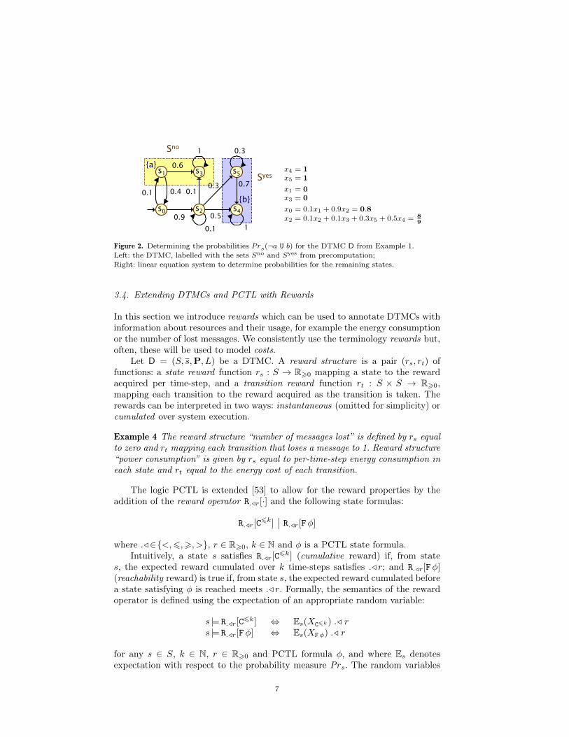
Example 3 Consider the DTMC D from Example 1 (see Figure 1) and the PCTL

formula P>0.8[¬a U b]. We have Sno = s1, s3 and Syes = s4, s5. These sets,

and the resulting linear equation system, are shown in Figure 2. This yields the

solution (0.8, 0, 89 , 0, 1, 1), and we see that Sat(P>0.8[¬a U b]) = s2, s4, s5.

6

Sno

a

b 0.4 0.1

0.6

1 0.3

0.7 0.1

0.3

0.9 1

Syes

0.1

0.5

s1 s3 s5

s0 s2 s4

x4 = 1x5 = 1

x1 = 0x3 = 0

x0 = 0.1x1 + 0.9x2 = 0.8x2 = 0.1x2 + 0.1x3 + 0.3x5 + 0.5x4 = 8

9

Figure 2. Determining the probabilities Prs(¬a U b) for the DTMC D from Example 1.Left: the DTMC, labelled with the sets Sno and Syes from precomputation;

Right: linear equation system to determine probabilities for the remaining states.

3.4. Extending DTMCs and PCTL with Rewards

In this section we introduce rewards which can be used to annotate DTMCs withinformation about resources and their usage, for example the energy consumptionor the number of lost messages. We consistently use the terminology rewards but,often, these will be used to model costs.

Let D = (S, s,P, L) be a DTMC. A reward structure is a pair (rs, rt) offunctions: a state reward function rs : S → R>0 mapping a state to the rewardacquired per time-step, and a transition reward function rt : S × S → R>0,mapping each transition to the reward acquired as the transition is taken. Therewards can be interpreted in two ways: instantaneous (omitted for simplicity) orcumulated over system execution.

Example 4 The reward structure “number of messages lost” is defined by rs equalto zero and rt mapping each transition that loses a message to 1. Reward structure“power consumption” is given by rs equal to per-time-step energy consumption ineach state and rt equal to the energy cost of each transition.

The logic PCTL is extended [53] to allow for the reward properties by theaddition of the reward operator R./r[·] and the following state formulas:

R./r[C6k]

∣∣ R./r[Fφ]

where ./∈<,6,>, >, r ∈ R>0, k ∈ N and φ is a PCTL state formula.Intuitively, a state s satisfies R./r[C

6k] (cumulative reward) if, from states, the expected reward cumulated over k time-steps satisfies ./ r; and R./r[Fφ](reachability reward) is true if, from state s, the expected reward cumulated beforea state satisfying φ is reached meets ./ r. Formally, the semantics of the rewardoperator is defined using the expectation of an appropriate random variable:

s |= R./r[C6k] ⇔ Es(XC6k) ./ r

s |= R./r[Fφ] ⇔ Es(XFφ) ./ r

for any s ∈ S, k ∈ N, r ∈ R>0 and PCTL formula φ, and where Es denotesexpectation with respect to the probability measure Prs. The random variables

7

XC6k , XFφ : Paths → R>0 corresponding to the two forms of the reward operatorare defined, for any path ω = s0s1s2 · · · ∈ Paths, as follows:

XC6k(ω)def=

0 if k = 0∑k−1

i=0 rs(si) + rt(si, si+1) otherwise

XFφ(ω)def=

0 if s0 |=φ∞ if ∀i ∈ N. si 6|=φ∑minj|sj |=φ−1i=0 rs(si) + rt(si, si+1) otherwise.

As for the probabilistic operator, if the outermost operator of a PCTL formulais R./r[·], we can omit the bound ./ r and compute the expected value instead.This also enables a range of such values to be obtained by varying one or moreparameters, either of the model or of the property.

Example 5 Below are some examples of reward based specifications:

• R=?[C610] - what is the expected number of messages lost within the first 10time-steps?;

• R65[F end ] - the expected time to termination is at most 5.

Model checking of the reward operator is similar to computing probabilities forthe probabilistic operator, and follows through the solution of recursive equations(for R./r[C

6k]) or a system of linear equations (for R./r[Fφ]). For more details onthis, and other aspects of probabilistic model checking for DTMCs, see e.g. [53,9].

3.5. More on Model Checking for DTMCs

The time complexity for PCTL model checking over DTMCs, including the rewardoperator, is linear in the size of the formula |φ| (number of logical connectivesand temporal operators) and polynomial in the size of the state space |S| [35].

DTMCs can also be verified against LTL properties, but the verificationmethod is quite different. The LTL formula is first translated into a Rabin automa-ton and then model checking reduces to the computation of probabilistic reacha-bility of bottom strongly connected components on the product of the DTMC andthe formula automaton [9]. The overall complexity for LTL is doubly exponentialin |φ| and polynomial in in |S|, but can be reduced to a single exponential.

4. Model Checking for Markov Decision Processes

We now explain how to model check Markov decision processes (MDPs), whichgeneralise discrete-time Markov chains with the addition of nondeterminism.Probability is employed to quantify aspects of system behaviour where probabilitydistributions are known. In contrast, nondeterminism is used to model unknownenvironments, where such distributions are not known. It is also used to modelconcurrency, where it represents the different possible interleavings of multiplecomponents operating in parallel. Alternatively, we can use nondeterminism tocapture the possible ways that a controller can influence the behaviour of thesystem, e.g. in planning and robotics.

8

s1 s0

s2

s3

0.5

0.5 0.7

1 1

heads

tails

init

0.3

1 a

bc

a

a

Figure 3. An example MDP.

4.1. Markov Decision Processes

Formally, we define a Markov decision process as follows.

Definition 3 (Markov decision process) A Markov decision process (MDP) is atuple M=(S, s,Act ,Steps, L) where S is a set of states, s ∈ S is an initial state,Act is an alphabet of actions, Steps : S×Act → Dist(S) is a (partial) probabilistictransition function and L : S → 2AP is a labelling function mapping each stateto a set of atomic propositions taken from a set AP.

In an MDP, several actions may be available in a given state s, each cor-responding to a probability distribution. We denote this set by A(s) = a ∈Act | Steps(s, a) is defined. As for DTMCs, we disallow deadlocks, and henceassume that A(s) is non-empty for all s ∈ S. The behaviour of an MDP M is asfollows. Firstly, a choice between one or more actions from the alphabet Act ismade nondeterministically. Secondly, for the chosen action a, a successor state s′

is chosen randomly, according to the probability distribution Steps(s, a), i.e. theprobability that a transition to s′ occurs is Steps(s, a)(s′).

An infinite path through an MDP is a sequence ω=s0a0s1a1 . . . where si ∈ S,ai ∈ A(si) and Steps(si, ai)(si+1)>0 for all i ∈ N. A finite path π=s0a0s1 . . . snis a prefix of an infinite path ending in a state. We denote by Paths and Pathfin

s

the sets of all infinite and finite paths from state s, respectively, and by Path andPathfin the corresponding sets of paths from any state. For a finite path π, thelast state of π is denoted last(π).

Example 6 Figure 3 shows an example MDP M = (S, s,Act ,Steps, L) with statesS = s0, . . . , s3, initial state s0 and alphabet of actions a, b, c. State s1, forexample, has a nondeterministic choice between two actions, b and c.

To reason formally about MDPs, we need a probability space over infinitepaths. However, a probability space can only be constructed once all the nonde-terminism has been resolved. Each possible resolution of nondeterminism is rep-resented by an adversary, also called a policy, which is responsible for choosingan action in each state of the MDP, based on the history of its execution so far.

Definition 4 (Adversary) An adversary of an MDP M = (S, s,Act ,Steps, L) is afunction σ : Pathfin→Dist(Act) such that σ(π)(a)>0 only if a ∈ A(last(π)). Anadversary σ is memoryless if σ(π) depends only on last(π) and deterministic ifthe distribution σ(π) always selects a single action with probability 1.

9

s0

0.5

1

s0s1s0s1s2

s0s1s0s1s3 0.5 s0s1

0.7 s0s1s0

s0s1s1 0.3

1 s0s1s0s1

0.5 s0s1s1s2

s0s1s1s3 0.5

1

1

s0s1s1s2s2

s0s1s1s3s3

Figure 4. The induced DTMC for an adversary of the MDP in Figure 3.

The set of all adversaries of an MDP M is denoted Adv . Under a particularadversary σ ∈ Adv , the behaviour of M is fully probabilistic and can be capturedby an induced DTMC, denoted Mσ, each state of which is a finite path of M.

Definition 5 (Induced DTMC) For an MDP M = (S, s,Act ,Steps, L) and adver-sary σ, the induced DTMC is Mσ = (Pathfin, s,P, L′) where:

• for any π, π′ ∈ Pathfin:

P(π, π′) =

σ(π)(a) · Steps(last(π), a)(s) if π′ = πas, a ∈ A(last(π))0 otherwise;

• L′(π) = L(last(π)) for all π ∈ Pathfin.

Notice that there is a one-to-one mapping between the infinite paths of the DTMCMσ and the infinite paths of MDP M when under the control of adversary σ. Thismeans that the DTMC yields, for a start state s, a probability space, denotedPrσs over these infinite paths. The induced DTMC Mσ has a (countably) infinitenumber of states. However, in the case of memoryless adversaries, its state spaceis isomorphic to S and Mσ can be reduced to an |S|-state DTMC.

Example 7 Consider the MDP M from Example 6 (shown in Figure 3) and the(deterministic, but non-memoryless) adversary σ, which picks action b the firsttime that state s1 is reached, and then action c the second time. The inducedDTMC Mσ is shown in Figure 4.

4.2. PCTL Model Checking over MDPs

Probabilistic statements about MDPs typically involve quantification over adver-saries, so as to establish that some specified event is observed for all possible ad-versaries. The logic PCTL, for example, is defined for MDPs as for DTMCs [14],the key difference being that the semantics of the probabilistic operator containsexplicit universal quantification:

s |= P./ p[ψ] ⇔ Prσs ω ∈ Paths | ω |= ψ ./ p for all σ ∈ Adv.

The algorithm for PCTL model checking proceeds as for DTMCs, except forthe probabilistic operator. For P. p[ψ] where . ∈ >, >, this reduces to the

10

calculation of the minimum probability Prmins (ψ). The case of P/ p[ψ] for / ∈ 6

, < is dual, via the maximum probability Prmaxs (ψ):

Sat(P. p[ψ]) = s ∈ S | Prmins (ψ) . p

Sat(P/ p[ψ]) = s ∈ S | Prmaxs (ψ) / p

where Prmins (ψ) = infσ∈AdvPrσs (ψ) and Prmax

s (ψ) = supσ∈AdvPrσs (ψ).

To describe the computation of these values, we restrict our attention to the caseof minimum probabilities. If ψ = Xφ, we have:

Prmins (Xφ) = mina∈A(s)

[∑s′∈Sat(φ) Steps(s, a)(s′)

].

For ψ = φ1 U φ2, the minimum probabilities are the unique solution of:

Prmins (ψ) =

0 if s ∈ Sno1 if s ∈ Syesmina∈A(s)

[∑s′∈S Steps(s, a)(s′) · Prmin

s′ (ψ)]

if s ∈ S?

with Sno and Syes denoting the sets of states where the minimum probability isrespectively 0 and 1, precomputed in a similar fashion to the DTMC case via afixpoint (see e.g. [28]). The computation of these probabilities can be performedin several different ways; we detail three such methods below.

Linear programming. The minimum probabilities Prmins (φ1 U φ2) for s ∈ S can

be obtained as the unique solution of the following linear program (LP):

maximise∑s∈S xs subject to the constraints:

xs = 0 for all s ∈ Snoxs = 1 for all s ∈ Syesxs 6

∑s′∈S Steps(s, a)(s′) · xs′ for all s ∈ S? and a ∈ A(s) .

This can be solved using standard techniques such as the simplex, ellipsoid orbranch-and-cut methods.

Value iteration. The minimum probabilities can also be approximated iteratively,

since Prmins (φ1 U φ2) = limn→∞ x

(n)s , as follows:

x(n)s =

0 if s ∈ Sno1 if s ∈ Syes0 if s ∈ S? and n = 0

mina∈A(s)

∑s′∈S Steps(s, a)(s′) · x(n−1)

s′

if s ∈ S? and n > 0 .

In practice, the iterative computation is terminated when the values x(n)s have

converged sufficiently with respect to a given level of precision ε > 0.

Policy iteration. This method iterates over adversaries (i.e. policies), as opposedto probability values. It starts with an arbitrary, memoryless adversary σ andcomputes the probability pσs of satisfying φ1 U φ2 from each state s under σ. This

11

s0

s1 s2

s3

0.5

0.25

1

1

1

a

0.4

0.5

0.1

0.25

1

Syes

Sno

(a) Example MDP, labelled

with the sets Sno and Syes

from precomputation.

x0

x1

0

0

1

1

0.8

2/3

max

(b) Linear programming problem

yielding minimum probabilities ofreaching a-labelled states.

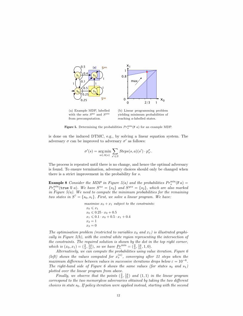
Figure 5. Determining the probabilities Prmins (F a) for an example MDP.

is done on the induced DTMC, e.g., by solving a linear equation system. Theadversary σ can be improved to adversary σ′ as follows:

σ′(s) = arg mina∈A(s)

∑s′∈S

Steps(s, a)(s′) · pσs′ .

The process is repeated until there is no change, and hence the optimal adversaryis found. To ensure termination, adversary choices should only be changed whenthere is a strict improvement in the probability for s.

Example 8 Consider the MDP in Figure 5(a) and the probabilities Prmins (F a) =

Prmins (true U a). We have Sno = s3 and Syes = s2, which are also marked

in Figure 5(a). We need to compute the minimum probabilities for the remainingtwo states in S? = s0, s1. First, we solve a linear program. We have:

maximise x0 + x1 subject to the constraints:x0 6 x1

x0 6 0.25 · x0 + 0.5x1 6 0.1 · x0 + 0.5 · x1 + 0.4x2 = 1x3 = 0

The optimisation problem (restricted to variables x0 and x1) is illustrated graphi-cally in Figure 5(b), with the central white region representing the intersection ofthe constraints. The required solution is shown by the dot in the top right corner,which is (x0, x1) = (2

3 ,1415 ), so we have Prmin = ( 2

3 ,1415 , 1, 0).

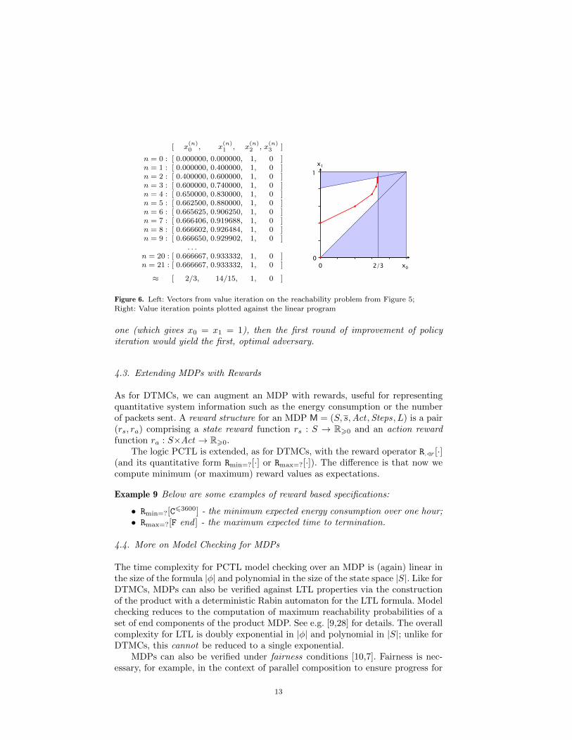
Alternatively, we can compute the probabilities using value iteration. Figure 6

(left) shows the values computed for x(n)s , converging after 21 steps when the

maximum difference between values in successive iterations drops below ε = 10−6.The right-hand side of Figure 6 shows the same values (for states s0 and s1)plotted over the linear program from above.

Finally, we observe that the points ( 23 ,

1415 ) and (1, 1) in the linear program

correspond to the two memoryless adversaries obtained by taking the two differentchoices in state s0. If policy iteration were applied instead, starting with the second

12

[ x(n)0 , x

(n)1 , x

(n)2 , x

(n)3 ]

n = 0 : [ 0.000000, 0.000000, 1, 0 ]n = 1 : [ 0.000000, 0.400000, 1, 0 ]n = 2 : [ 0.400000, 0.600000, 1, 0 ]n = 3 : [ 0.600000, 0.740000, 1, 0 ]n = 4 : [ 0.650000, 0.830000, 1, 0 ]n = 5 : [ 0.662500, 0.880000, 1, 0 ]n = 6 : [ 0.665625, 0.906250, 1, 0 ]n = 7 : [ 0.666406, 0.919688, 1, 0 ]n = 8 : [ 0.666602, 0.926484, 1, 0 ]n = 9 : [ 0.666650, 0.929902, 1, 0 ]

. . .n = 20 : [ 0.666667, 0.933332, 1, 0 ]n = 21 : [ 0.666667, 0.933332, 1, 0 ]

≈ [ 2/3, 14/15, 1, 0 ]

x0

x1

0

0 2/3

1

Figure 6. Left: Vectors from value iteration on the reachability problem from Figure 5;

Right: Value iteration points plotted against the linear program

one (which gives x0 = x1 = 1), then the first round of improvement of policyiteration would yield the first, optimal adversary.

4.3. Extending MDPs with Rewards

As for DTMCs, we can augment an MDP with rewards, useful for representingquantitative system information such as the energy consumption or the numberof packets sent. A reward structure for an MDP M = (S, s,Act ,Steps, L) is a pair(rs, ra) comprising a state reward function rs : S → R>0 and an action rewardfunction ra : S×Act → R>0.

The logic PCTL is extended, as for DTMCs, with the reward operator R./r[·](and its quantitative form Rmin=?[·] or Rmax=?[·]). The difference is that now wecompute minimum (or maximum) reward values as expectations.

Example 9 Below are some examples of reward based specifications:

• Rmin=?[C63600] - the minimum expected energy consumption over one hour;• Rmax=?[F end ] - the maximum expected time to termination.

4.4. More on Model Checking for MDPs

The time complexity for PCTL model checking over an MDP is (again) linear inthe size of the formula |φ| and polynomial in the size of the state space |S|. Like forDTMCs, MDPs can also be verified against LTL properties via the constructionof the product with a deterministic Rabin automaton for the LTL formula. Modelchecking reduces to the computation of maximum reachability probabilities of aset of end components of the product MDP. See e.g. [9,28] for details. The overallcomplexity for LTL is doubly exponential in |φ| and polynomial in |S|; unlike forDTMCs, this cannot be reduced to a single exponential.

MDPs can also be verified under fairness conditions [10,7]. Fairness is nec-essary, for example, in the context of parallel composition to ensure progress for

13

each concurrent component whenever possible. For modelling and verification ofprobabilistic systems comprising multiple components, the closely related modelof probabilistic automata has been developed, along with rich theories for compo-sitional modelling and analysis [61].

5. Quantitative Abstraction Refinement

The techniques described in the preceding two sections can be used to establisha wide range of useful properties of systems modelled as DTMCs and MDPs.Furthermore, these methods are efficient: typically the time complexity is poly-nomial in the size of the state space of the model. In practice, though, one of theprincipal challenges in applying probabilistic model checking to real-life systemsis scalability : the models that need to be constructed and analysed are often sim-ply too big for the process to be feasible. This phenomenon, commonly called thestate-space explosion problem, affects all verification approaches that rely on anexhaustive analysis of a model’s state space.

In this section, we describe the use of abstraction as a mechanism for over-coming the state-space explosion problem. Abstraction techniques work by hid-ing aspects of the system being modelled that are not relevant to the propertycurrently being verified, resulting in a smaller abstract model. Let us refer to thestates s ∈ S of the model that is to be abstracted as concrete states. We willdefine an abstraction of the model based on a partition A of these concrete states,with each subset in the partition referred to as an abstract state a ∈ A. We thenbuild an abstract model, whose state space is the set of abstract states A.

5.1. Abstracting MDPs as Stochastic Games

In this tutorial, we will focus on the problem of building abstractions for Markovdecisions processes (MDPs), since this is the more general of the two modelsthat we have considered. One approach to defining an abstraction of an MDP M,based on a partition A of its states into abstract states, is to use an existentialabstraction [22], which takes the form of another MDP MA with state space A.

The existential abstraction MA is built by lifting each probability distribu-tion µ (over S) in MDP M to a distribution µA over A, i.e. for each a ∈ A,µA(a) =

∑s∈a µ(a). For each abstract state a in MA, Steps(a) then contains the

distributions µA for all distributions µ from any state s such that s ∈ a.

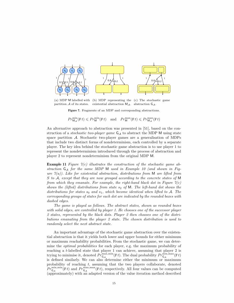
Example 10 Figure 7(a) shows a fragment of an MDP M, annotated with a par-tition A of its states. Figure 7(b) shows the corresponding fragment of the exis-tential abstraction MA.

Formally, the MDP M and its abstraction MA are related through strongsimulation [62], which means that the abstraction preserves the “safe” fragmentof PCTL. Furthermore, MA yields bounds on the reachability probabilities for M.More precisely, letting t be an atomic proposition labelling a target abstract statein MA, we can obtain a lower bound on the minimum probability of reaching tand an upper bound on the maximum probability of reaching it:

14

0.5 0.1 0.8 1

0.5 1

0.1

1

s0 s1 s2

s3 s4 s5 s6

(a) MDP M labelled withpartition A of its states.

1 1 0.2 0.8

(b) MDP representing theexistential abstraction MA.

1 1 0.2 0.8

(c) The stochastic gameabstraction GA.

Figure 7. Fragments of an MDP and corresponding abstractions.

PrminMA

(F t) 6 PrminM (F t) and Prmax

M (F t) 6 PrmaxMA

(F t)

An alternative approach to abstraction was presented in [51], based on the con-struction of a stochastic two-player game GA to abstract the MDP M using statespace partition A. Stochastic two-player games are a generalisation of MDPsthat include two distinct forms of nondeterminism, each controlled by a separateplayer. The key idea behind the stochastic game abstraction is to use player 1 torepresent the nondeterminism introduced through the process of abstraction andplayer 2 to represent nondeterminism from the original MDP M.

Example 11 Figure 7(c) illustrates the construction of the stochastic game ab-straction GA for the same MDP M used in Example 10 (and shown in Fig-ure 7(a)). Like for existential abstraction, distributions from M are lifted fromS to A, except that they are now grouped according to the concrete states of Mfrom which they emanate. For example, the right-hand black dot in Figure 7(c)shows the (lifted) distributions from state s2 of M. The left-hand dot shows thedistributions for states s0 and s1, which become identical when lifted to A. Thecorresponding groups of states for each dot are indicated by the rounded boxes withdashed edges.

The game is played as follows. The abstract states, shown as rounded boxeswith solid edges, are controlled by player 1. He chooses one of the successor player2 states, represented by the black dots. Player 2 then chooses one of the distri-butions emanating from the player 2 state. The chosen distribution is used torandomly select the next abstract state.

An important advantage of the stochastic game abstraction over the existen-tial abstraction is that it yields both lower and upper bounds for either minimumor maximum reachability probabilities. From the stochastic game, we can deter-mine the optimal probabilities for each player, e.g. the maximum probability ofreaching a t-labelled state that player 1 can achieve, assuming that player 2 istrying to minimise it, denoted Prmax,min

GA(F t). The dual probability Prmin,max

GA(F t)

is defined similarly. We can also determine either the minimum or maximumprobability of reaching t, assuming that the two players collaborate, denotedPrmin,min

GA(F t) and Prmax,max

GA(F t), respectively. All four values can be computed

(approximately) with an adapted version of the value iteration method described

15

(a) Self-stabilisation protocol. (b) Sliding window protocol.

Figure 8. Graphs illustrating the lower and upper bounds obtained from the stochastic gameabstractions of MDPs from two large case studies.

in Section 4.2 for MDPs. The values, when computed for the stochastic gameabstraction GA of an MDP M, yield lower and upper bounds as follows:

Prmin,minGA

(F t) 6 PrminM (F t) 6 Prmax,min

GA(F t)

Prmin,maxGA

(F t) 6 PrmaxM (F t) 6 Prmax,max

GA(F t)

Figure 8 shows some typical examples of these bounds, obtained from real casestudies [45]. Part (a) plots results for the “minimum probability of terminationwithin time T” on a model of Israeli & Jalfon’s self-stabilisation protocol, fora range of values of T . In this case, the MDP has 1,048,575 states, whereasthe stochastic game abstraction has only 627. Part (b) shows results for “themaximum probability of K time-outs” on a model of a sliding window protocol,varying both K and the number frames sent D. In this case, we see that the lowerand upper bounds are tight, yielding the exact answers. Also, in this example, theuse of predicate abstraction allows us to build and analyse abstractions for MDPsthat are too large to verify directly. Thus, we see results on the right-hand sideof the graph that could not have been obtained without the use of abstraction.

5.2. Quantitative Abstraction Refinement

Although the stochastic game abstractions presented above were constructed andanalysed in a fully automated fashion, one crucial part of the process was stillperformed manually: the specification of the abstract state space A. The practicalapplicability and usefulness of the abstraction techniques are completely relianton being able to determine an appropriate partition A of the concrete state space,i.e. one that is coarse enough to yield a small abstract model, but which giveslower and upper bounds that are close enough to provide useful information.

Here, we discuss a way to construct such a partition A in a fully auto-matic fashion, using abstraction refinement. This is inspired by the successfulcounterexample-guided abstraction refinement (CEGAR) approach [20], developedto build abstractions for non-probabilistic model checking. The idea is to startwith a simple, coarse partition, build the corresponding abstraction, and theniteratively refine the partition, resulting in increasingly precise abstractions. InCEGAR, the refinement step is driven by counterexamples obtained by model

16

partition AMDP M,

error bound εtarget t,

build abstraction(stoch. game GA)

error>ε

abstractionrefine

returnbounds

error<εmodel checkgame GA

Figure 9. Quantitative abstraction-refinement loop.

checking the abstractions produced at each iteration, and the iterations of refine-ment are terminated when the current abstraction can be used either to verify orrefute the property being verified.

Here, we describe quantitative abstraction refinement [47], which can be seenas a quantitative analogue of CEGAR, applied to the stochastic game abstractionapproach of [51]. The idea is that the difference between the lower and upperbounds obtained from an abstraction (which we call the “error”) quantifies theprecision of the abstraction. If the error is too high, the abstraction should berefined (i.e. a finer partition A used).

Figure 9 shows a quantitative abstraction-refinement loop used to automat-ically construct stochastic game abstractions of an MDP M. Starting with aninitial (coarse) partition, abstractions are repeatedly constructed, analysed andrefined until the difference between the lower and upper bounds obtained forthe property of interest (say, the minimum or maximum probability of reachingt-labelled states) falls below some threshold ε.

The applicability of quantitative abstraction refinement was initially demon-strated in [47], on a simple explicit-state implementation, applied to a set ofbenchmark models. Subsequently, the approach has been successfully applied tothe verification of:

• probabilistic real-time systems, modelled using probabilistic timed au-tomata [54] (see the next section for a more in-depth discussion);

• probabilistic software, based on the use of ANSI-C code, augmented withprobabilistic commands [46];

• concurrent probabilistic programs, as analysed by the probabilistic abstrac-tion tool PASS [29];

• probabilistic programs over arbitrary abstract domains [27];• probabilistic hybrid automata [31].

Several other methods for abstraction refinement of probabilistic systems havealso been proposed [22,41,25,16]; see e.g. [47] for a discussion of the differencesbetween these approaches.

6. Probabilistic Timed Automata

The two models that we presented in the first half of this tutorial, DTMCs andMDPs, both use a discrete model of time, i.e. a system execution is modelledas a sequence of discrete time-steps. In this section, we discuss modelling andverification of probabilistic real-time systems, which use a continuous (dense)model of time. These systems will be modelled by probabilistic timed automata.

17

Another popular model incorporating a continuous notion of time is continuous-time Markov chains (CTMCs), an extension of DTMCs where the delays betweenstate transitions are represented by exponential distributions. See, for example,[8,53] for overviews of probabilistic model checking techniques for CTMCs.

6.1. Probabilistic Timed Automata

Probabilistic timed automata (PTAs) [42,59] model systems that exhibit prob-abilistic, nondeterministic and real-time characteristics. They can be seen as anextension of MDPs with clocks, real-valued variables whose values increase simul-taneously over time. Like in the classic model of timed automata [2], states andtransitions of PTAs can be labelled with invariants and guards, that is, predi-cates on clocks respectively dictating how long to remain in a state and whentransitions can occur. Transitions between states (represented, as in MDPs, byprobability distributions) can also reset the values of one or more clocks.

To specify invariants and guards, we use clock constraints. Assuming a set ofclocks X , the set of allowable clock constraints, denoted CC (X ), is defined by thefollowing grammar:

χ ::= true | x 6 d | c 6 x | x+c 6 y+d | ¬χ | χ ∧ χ

where x, y ∈ X and c, d ∈ N. A PTA can then be formally defined as follows.

Definition 6 (Probabilistic timed automaton) A probabilistic timed automaton(PTA) is defined by a tuple P=(Loc, l,X ,Act , inv , enab, prob, L) where:

• Loc is a finite set of locations;• l ∈ Loc is an initial location;• X is a finite set of clocks;• Act is a finite set of actions;• inv : Loc → CC (X ) is the invariant condition;• enab : Loc×Act → CC (X ) is the enabling condition;• prob : Loc×Act → Dist(2X×Loc) is a (partial) probabilistic transition

function;• L : Loc → 2AP is a labelling function mapping each location to a set of

atomic propositions taken from a set AP.

The semantics of a PTA P is given by an infinite-state MDP whose states areof the form (l, v) ∈ Loc×(R>0)

X, where l is a location and v gives a value for each

clock in X . For simplicity, we omit a full descriptions of the semantics (see e.g.[58] for details). Intuitively, the behaviour of a PTA is as follows. The initial stateis (l,0), where 0 denotes a value of 0 for all clocks. For a general state s = (l, v),there is a nondeterministic choice between either: (i) time elapsing, i.e. all clocksincreasing in value, subject to the invariant inv(l) staying true; (ii) an action abeing taken, such that prob(l, a) is defined and the guard enab(l, a) is satisfied.If the latter, prob(l, a) is a distribution over pairs (X, l′) ∈ 2X × Loc, giving theprobability of moving to location l′ and resetting the clocks in X to zero.

18

init x=0

0.9

retry

done true

lost x!5

c++

fail true

give-"up

time "out

y>4 c>5 send

x#3

x:=0

c!5$y!4 0.1

c:=0

Figure 10. Example PTA.

Example 12 Figure 10 shows an example of a PTA with locations Loc =init, lost,done, fail and two clocks x, y. Locations are labelled with their in-variants, under the location name, and transitions are annotated with actions(from the set Act = send , retry , giveup, timeout), guards (e.g. y > 4), clockresets (e.g. x := 0) and probabilities. For modelling convenience, we also use aninteger variable c, whose value can feature in guards or be set on a transition.

The PTA models repeated attempts to transmit a message over a faulty com-munication channel. Each send happens instantaneously (thanks to the invariantx = 0 in location init), after which the transmission succeeds with probability 0.9and fails with probability 0.1. In the case of failure, a delay of between 3 and 5time units occurs before transmission is re-attempted. The variable c counts thenumber of attempts. If either c exceeds 5, or the total time elapsed (stored by clocky) exceeds 4, then transmission is aborted and the PTA moves to location fail.

6.2. Model Checking for PTAs

A variety of model checking approaches have been proposed for PTAs. Propertiesto be verified are typically expressed in probabilistic temporal logic. One possibil-ity is the logic PTCTL [59], a probabilistic extension of the timed temporal logicTCTL. In many cases, though, the simpler logic PCTL, discussed earlier in thistutorial for DTMCs and MDPs, suffices.

The principle hurdle to overcome when developing model checking algorithmsfor PTAs is the fact that the models are inherently infinite-state. Fundamentalresults about the decidability and complexity of model checking for PTAs canbe obtained through the construction of a region graph [59]. This is based on adivision of the PTA’s state space into a finite number of regions, sets of stateswhich satisfy exactly the same temporal logic formulas. This reduces the problemof model checking a PTA to the problem of analysing a finite-state MDP, whosestates are regions. In practice, however the region graph is prohibitively large,and thus several more efficient methods have been developed for model checking:

• The digital clocks method [57] translates closed PTAs (those where clockconstraints contain no strict comparisons) into a finite-state MDP, basedon the digitisation of real-valued to integer-valued clocks. The MDP is thenanalysed in standard fashion. For PTAs whose clock values vary across largeranges this approach can become expensive, but it has been successfullyapplied to several large case studies.

19

init, c=0, !x=y=0 fail, c=1, !

x=0,4<y"5

lost, c=2, !x=0,3"y"4

done, c=1, !x=0,3"y"4

init, c=2, !x=0,6"y"9

0.9 fail, c=2, !x=0,6"y"9

init, c=1, !x=0,3"y"5

done, c=0, !x=y=0

lost, c=1, !x=y=0 send

retry send

time-!out

time-!out

retry

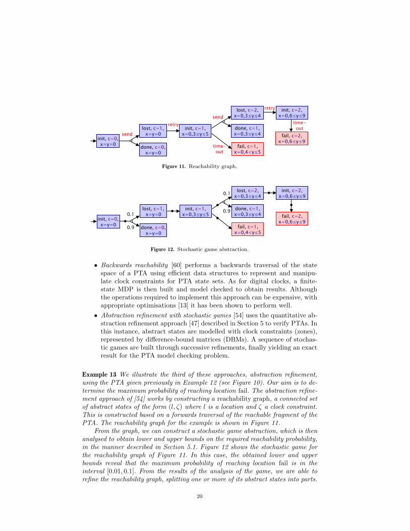
Figure 11. Reachability graph.

init, c=0, !x=y=0

0.1

0.9 fail, c=1, !x=0,4<y"5

lost, c=2, !x=0,3"y"4

done, c=1, !x=0,3"y"4

0.1

0.9

init, c=2, !x=0,6"y"9

0.9 fail, c=2, !x=0,6"y"9

init, c=1, !x=0,3"y"5

done, c=0, !x=y=0

lost, c=1, !x=y=0

Figure 12. Stochastic game abstraction.

• Backwards reachability [60] performs a backwards traversal of the statespace of a PTA using efficient data structures to represent and manipu-late clock constraints for PTA state sets. As for digital clocks, a finite-state MDP is then built and model checked to obtain results. Althoughthe operations required to implement this approach can be expensive, withappropriate optimisations [13] it has been shown to perform well.

• Abstraction refinement with stochastic games [54] uses the quantitative ab-straction refinement approach [47] described in Section 5 to verify PTAs. Inthis instance, abstract states are modelled with clock constraints (zones),represented by difference-bound matrices (DBMs). A sequence of stochas-tic games are built through successive refinements, finally yielding an exactresult for the PTA model checking problem.

Example 13 We illustrate the third of these approaches, abstraction refinement,using the PTA given previously in Example 12 (see Figure 10). Our aim is to de-termine the maximum probability of reaching location fail. The abstraction refine-ment approach of [54] works by constructing a reachability graph, a connected setof abstract states of the form (l, ζ) where l is a location and ζ a clock constraint.This is constructed based on a forwards traversal of the reachable fragment of thePTA. The reachability graph for the example is shown in Figure 11.

From the graph, we can construct a stochastic game abstraction, which is thenanalysed to obtain lower and upper bounds on the required reachability probability,in the manner described in Section 5.1. Figure 12 shows the stochastic game forthe reachability graph of Figure 11. In this case, the obtained lower and upperbounds reveal that the maximum probability of reaching location fail is in theinterval [0.01, 0.1]. From the results of the analysis of the game, we are able torefine the reachability graph, splitting one or more of its abstract states into parts.

20

For this example, a single refinement (which splits the clock constraint x=0 ∧36y65 in abstract state ((init, c=1), x=0 ∧ 36y65) into two, x=0 ∧ 36y64 andx=0∧4<y65) suffices to produce an abstraction which yields the bounds [0.1, 0.1].Thus, the maximum probability of failure is 0.1.

6.3. More on Model Checking for PTAs

As discussed previously for DTMCs and MDPs, we can augment PTAs with re-wards to capture additional quantitative properties of the models. In fact, theseare often used to model costs or prices. Computation of the (minimum or max-imum) expected reward cumulated until a target is reached can be performedusing the digital clocks method [57]. Another useful class of reward properties forPTAs is the probability that the cumulative reward exceeds a certain bound. Asemi-algorithm for model checking such properties can be found in [12].

7. Probabilistic Model Checking in Practice

We conclude this tutorial with a discussion of some of the practical aspects ofprobabilistic model checking. As usage of these techniques has become morewidespread, a variety of supporting software tools have been developed. The twomost widely used are PRISM [55] and MRMC [43]. MRMC’s core functionality ismodel checking of (discrete- and continuous-time) Markov chains, with a particu-lar focus on reward properties. PRISM supports Markov chains, as well as MDPsand PTAs, and is described in more detail below. Other tools providing modelchecking of MDPs include LiQuor [18] and ProbDiVinE [11]. Software supportingverification of PTAs includes UPPAAL-PRO [66], Fortuna [13] and mcpta [37]. Amore detailed list of probabilistic model checking tools can be found at [68].

7.1. PRISM

PRISM [55] is a probabilistic model checker developed at the Universities of Birm-ingham and Oxford. It is an open-source software tool which accepts probabilis-tic models written in a textual modelling language based on Reactive Modules,a state-based language using guarded commands. The three main model typesdiscussed in this tutorial, DTMCs, MDPs and PTAs, and their reward (price)extensions are all directly supported by PRISM, as are continuous-time Markovchains (CTMCs). A wide range of properties can be specified and model checked:PRISM admits the logics PCTL, LTL and PCTL*, and additionally CSL (forCTMCs). It also includes the reward operators and quantitative (numerical) prop-erties discussed earlier in this tutorial.

PRISM includes multiple model checking engines, notably several based onsymbolic implementations (using binary decision diagrams and their extensions).These can enable the probabilistic verification of models of up to 1010 states. Onaverage, the tool usually handles models with up to 107−108 states. PRISM alsofeatures explicit-state model checking functionality, as well as a variety of ad-vanced techniques such as abstraction refinement and symmetry reduction. There

21

is also support for approximate/statistical model checking through a discrete-event simulation engine.

PRISM has been applied to numerous case studies, from communication,security and population protocols, power management, embedded control, nan-otechnology designs, to biological systems; for more information consult [67].

7.2. Research Directions

Finally, we briefly mention some other directions for the development of proba-bilistic model checking that have shown promising results.

• Symbolic model checking techniques, using data structures based on bi-nary decision diagrams (BDDs) [5,49] offer scalability to large models byexploiting high-level structure and regularities.

• Model reduction techniques such as bisimulation minimisation [44], sym-metry reduction [52,26] and partial order reduction [23,6] provide waysto reduce the size of probabilistic models, whilst preserving exact modelchecking results.

• Compositional probabilistic verification [61] decomposes the effort requiredfor model checking into separate sub-tasks for each system component; inparticular, assume-guarantee verification techniques for MDPs [56] haverecently proved to provide real practical gains in scalability.

• Approximate (or statistical) probabilistic model checking improves scalabil-ity by combining Monte Carlo simulation with statistical methods to eithergenerate approximate results to quantitative model checking queries [39]or efficiently check properties featuring probability thresholds [65].

• Systems biology is proving to be an exciting and challenging application ofprobabilistic model checking, for which various novel techniques have beenspecifically developed [64,38].

• Probabilistic counterexamples [32,1,3] provide diagnostic information to theuser of a probabilistic model checker if a temporal logic query is found to befalse. Typically, this takes the form of a set of violating system executions,whose combined probability exceeds some desired threshold.

• Synthesis techniques aim to generate correct-by-construction model com-ponents or controllers based on quantitative objectives [17,15].

• Parametric approaches to probabilistic model checking can be used to syn-thesise the range of model parameter values that satisfy some specifica-tion [33] or to produce model checking results that are symbolic expressionsin terms of the parameters [30].

8. Conclusions

This tutorial presented an introduction to probabilistic model checking, coveringdetails of two basic models, Markov chains and Markov decision processes, and two

22

more advanced topics, quantitative abstraction refinement and model checkingof probabilistic timed automata. The focus has been on models which featurediscrete states, discrete probability distributions and possibly nondeterminism, inconjunction with (in the case of PTAs) dense real-time.

The following tutorial papers provide more comprehensive introductory ma-terial for the topics covered here:

• [53] (sections 1–3), for discrete-time Markov chains (DTMCs);• [28] (sections 1–7), for Markov decision processes (MDPs);• [58], for probabilistic timed automata (PTAs).

Chapter 10 of [9] is also highly recommended for additional and deeper coverageof model checking for DTMCs and MDPs.

Acknowledgments. The authors are part supported by ERC Advanced GrantVERIWARE, EPSRC grant EP/F001096/1 and EU-FP7 project CONNECT.

References

[1] H. Aljazzar and S. Leue. Directed explicit state-space search in the generation of coun-

terexamples for stochastic model checking. IEEE Transactions on Software Engineering,36(1):37–60, 2010.

[2] R. Alur and D. Dill. A theory of timed automata. Theoretical Computer Science, 126:183–

235, 1994.[3] M. Andres, P. D’Argenio, and P. van Rossum. Significant diagnostic counterexamples in

probabilistic model checking. In H. Chockler and A. Hu, editors, Proc. 4th Int. Haifa

Verification Conf. Hardware and Software: Verification and Testing (HVC’08), volume5394 of LNCS, pages 129–148. Springer, 2008.

[4] D. Angluin, J. Aspnes, and D. Eisenstat. A simple population protocol for fast robust

approximate majority. Distributed Computing, 21(2):87–102, 2008.[5] C. Baier, E. Clarke, V. Hartonas-Garmhausen, M. Kwiatkowska, and M. Ryan. Symbolic

model checking for probabilistic processes. In P. Degano, R. Gorrieri, and A. Marchetti-

Spaccamela, editors, Proc. 24th International Colloquium on Automata, Languages andProgramming (ICALP’97), volume 1256 of LNCS, pages 430–440. Springer, 1997.

[6] C. Baier, M. Groesser, and F. Ciesinski. Partial order reduction for probabilistic systems.In Proc. 1st International Conference on Quantitative Evaluation of Systems (QEST’04),

pages 230–239. IEEE CS Press, 2004.

[7] C. Baier, M. Großer, and F. Ciesinski. Quantitative analysis under fairness constraints.In Proc. 7th International Symposium on Automated Technology for Verification and

Analysis (ATVA’09), volume 5799 of LNCS, pages 135–150. Springer, 2009.[8] C. Baier, B. Haverkort, H. Hermanns, and J.-P. Katoen. Model-checking algorithms for

continuous-time Markov chains. IEEE Transactions on Software Engineering, 29(6):524–

541, 2003.

[9] C. Baier and J.-P. Katoen. Principles of Model Checking. MIT Press, 2008.[10] C. Baier and M. Kwiatkowska. Model checking for a probabilistic branching time logic

with fairness. Distributed Computing, 11(3):125–155, 1998.[11] J. Barnat, L. Brim, I. Cerna, M. Ceska, and J. Tumova. ProbDiVinE-MC: Multi-core

LTL model checker for probabilistic systems. In Proc. 5rd International Conference on

Quantitative Evaluation of Systems (QEST’08), pages 77–78. IEEE CS Press, 2008.[12] J. Berendsen, D. Jansen, and J.-P. Katoen. Probably on time and within budget – on

reachability in priced probabilistic timed automata. In Proc. 3rd International Conference

on Quantitative Evaluation of Systems (QEST’06), pages 311–322. IEEE CS Press, 2006.[13] J. Berendsen, D. Jansen, and F. Vaandrager. Fortuna: Model checking priced probabilistic

timed automata. In Proc. 7th International Conference on Quantitative Evaluation of

SysTems (QEST’10), pages 273–281, 2010.

23

[14] A. Bianco and L. de Alfaro. Model checking of probabilistic and nondeterministic systems.

In P. Thiagarajan, editor, Proc. 15th Conference on Foundations of Software Technologyand Theoretical Computer Science (FSTTCS’95), volume 1026 of LNCS, pages 499–513.

Springer, 1995.

[15] P. Cerny, K. Chatterjee, T. Henzinger, A. Radhakrishna, and R. Singh. Quantitativesynthesis for concurrent programs. In G. Gopalakrishnan and S. Qadeer, editors, Proc.

23rd International Conference on Computer Aided Verification (CAV’11), volume 6806

of LNCS, pages 243–259. Springer, 2011.[16] R. Chadha and M. Viswanathan. A counterexample guided abstraction-refinement frame-

work for Markov decision processes. ACM Transactions on Computational Logic, 12(1):1–49, 2010.

[17] K. Chatterjee, T. Henzinger, B. Jobstmann, and R. Singh. Measuring and synthesiz-

ing systems in probabilistic environments. In Proc. 22nd International Conference onComputer Aided Verification (CAV’10), LNCS. Springer, 2010.

[18] F. Ciesinski and C. Baier. Liquor: A tool for qualitative and quantitative linear time analy-

sis of reactive systems. In Proc. 3rd International Conference on Quantitative Evaluationof Systems (QEST’06), pages 131–132. IEEE CS Press, 2006.

[19] E. Clarke and A. Emerson. Design and synthesis of synchronization skeletons using branch-

ing time temporal logic. In Proc. Workshop on Logic of Programs, volume 131 of LNCS.Springer, 1981.

[20] E. Clarke, O. Grumberg, S. Jha, Y. Lu, and H. Veith. Counterexample-guided abstraction

refinement. In A. Emerson and A. Sistla, editors, Proc. 12th Int. Conf. Computer AidedVerification (CAV’00), volume 1855 of Lecture Notes in Computer Science, pages 154–169.

Springer, 2000.[21] C. Courcoubetis and M. Yannakakis. Verifying temporal properties of finite state proba-

bilistic programs. In Proc. 29th Annual Symposium on Foundations of Computer Science

(FOCS’88), pages 338–345. IEEE Computer Society Press, 1988.[22] P. D’Argenio, B. Jeannet, H. Jensen, and K. Larsen. Reachability analysis of probabilistic

systems by successive refinements. In L. de Alfaro and S. Gilmore, editors, Proc. 1st

Joint International Workshop on Process Algebra and Probabilistic Methods, PerformanceModelling and Verification (PAPM/PROBMIV’01), volume 2165 of LNCS, pages 39–56.

Springer, 2001.

[23] P. D’Argenio and P. Niebert. Partial order reduction on concurrent probabilistic programs.In Proc. 1st International Conference on Quantitative Evaluation of Systems (QEST’04).

IEEE CS Press, 2004.

[24] L. de Alfaro, M. Kwiatkowska, G. Norman, D. Parker, and R. Segala. Symbolic modelchecking of probabilistic processes using MTBDDs and the Kronecker representation. In

S. Graf and M. Schwartzbach, editors, Proc. 6th International Conference on Tools andAlgorithms for the Construction and Analysis of Systems (TACAS’00), volume 1785 of

LNCS, pages 395–410. Springer, 2000.

[25] L. de Alfaro and P. Roy. Magnifying-lens abstraction for Markov decision processes. InProc. 19th International Conference on Computer Aided Verification (CAV’07), volume

4590 of LNCS, pages 325–338. Springer, 2007.[26] A. Donaldson and A. Miller. Symmetry reduction for probabilistic model checking using

generic representatives. In S. Graf and W. Zhang, editors, Proc. 4th Int. Symp. Automated

Technology for Verification and Analysis (ATVA’06), volume 4218 of Lecture Notes in

Computer Science, pages 9–23. Springer, 2006.[27] J. Esparza and A. Gaiser. Probabilistic abstractions with arbitrary domains. In Proc.

18th International Symposium on Static Analysis (SAS’11), pages 334–350, 2011.[28] V. Forejt, M. Kwiatkowska, G. Norman, and D. Parker. Automated verification techniques

for probabilistic systems. In M. Bernardo and V. Issarny, editors, Formal Methods for

Eternal Networked Software Systems (SFM’11), volume 6659 of LNCS, pages 53–113.

Springer, 2011.[29] E. M. Hahn, H. Hermanns, B. Wachter, and L. Zhang. PASS: Abstraction refinement

for infinite probabilistic models. In J. Esparza and R. Majumdar, editors, Proc. 16thInternational Conference on Tools and Algorithms for the Construction and Analysis of

24

Systems (TACAS’10), volume 6105 of LNCS, pages 353–357. Springer, 2010.

[30] E. M. Hahn, H. Hermanns, and L. Zhang. Probabilistic reachability for parametric Markovmodels. In C. Pasareanu, editor, Proc. 16th International SPIN Workshop, volume 5578

of LNCS, pages 88–106. Springer, 2009.

[31] E. M. Hahn, G. Norman, D. Parker, B. Wachter, and L. Zhang. Game-based abstractionand controller synthesis for probabilistic hybrid systems. In Proc. 8th International Con-

ference on Quantitative Evaluation of SysTems (QEST’11), pages 69–78. IEEE CS Press,

September 2011.[32] T. Han, J.-P. Katoen, and B. Damman. Counterexample generation in probabilistic model

checking. IEEE Transactions on Software Engineering, 35(2):241–257, 2009.[33] T. Han, J.-P. Katoen, and A. Mereacre. Approximate parameter synthesis for probabilistic

time-bounded reachability. In Proc. IEEE Real-Time Systems Symposium (RTSS 08),

pages 173–182. IEEE CS Press, 2008.[34] H. Hansson. Time and Probability in Formal Design of Distributed Systems. Elsevier,

1994.

[35] H. Hansson and B. Jonsson. A logic for reasoning about time and reliability. FormalAspects of Computing, 6(5):512–535, 1994.

[36] S. Hart, M. Sharir, and A. Pnueli. Termination of probabilistic concurrent programs.

ACM Transactions on Programming Languages and Systems, 5(3):356–380, 1983.[37] A. Hartmanns and H. Hermanns. A modest approach to checking probabilistic timed

automata. In Proc. 6th International Conference on Quantitative Evaluation of Systems

(QEST’09), 2009. To appear.[38] T. Henzinger, M. Mateescu, L. Mikeev, and V. Wolf. Hybrid numerical solution of the

chemical master equation. In Proc. 8th International Conference on Computational Meth-ods in Systems Biology (CMSB’10), pages 55–65. ACM, 2010.

[39] T. Herault, R. Lassaigne, F. Magniette, and S. Peyronnet. Approximate probabilistic

model checking. In Proc. 5th International Conference on Verification, Model Checkingand Abstract Interpretation (VMCAI’04), volume 2937 of LNCS. Springer, 2004.

[40] H. Hermanns, J.-P. Katoen, J. Meyer-Kayser, and M. Siegle. A Markov chain model

checker. In S. Graf and M. Schwartzbach, editors, Proc. 6th International Conference onTools and Algorithms for the Construction and Analysis of Systems (TACAS’00), volume

1785 of LNCS, pages 347–362. Springer, 2000.

[41] H. Hermanns, B. Wachter, and L. Zhang. Probabilistic CEGAR. In A. Gupta and S. Malik,editors, Proc. 20th International Conference on Computer Aided Verification (CAV’08),

volume 5123 of LNCS, pages 162–175. Springer, 2008.

[42] H. Jensen. Model checking probabilistic real time systems. In Proc. 7th Nordic Workshopon Programming Theory, pages 247–261, 1996.

[43] J.-P. Katoen, E. M. Hahn, H. Hermanns, D. Jansen, and I. Zapreev. The ins and outsof the probabilistic model checker MRMC. In Proc. 6th International Conference on

Quantitative Evaluation of Systems (QEST’09), pages 167–176. IEEE CS Press, 2009.

[44] J.-P. Katoen, T. Kemna, I. Zapreev, and D. Jansen. Bisimulation minimisation mostlyspeeds up probabilistic model checking. In O. Grumberg and M. Huth, editors, Proc. 13th

International Conference on Tools and Algorithms for the Construction and Analysis ofSystems (TACAS’07), volume 4424 of LNCS, pages 87–101. Springer, 2007.

[45] M. Kattenbelt, M. Kwiatkowska, G. Norman, and D. Parker. Game-based probabilis-

tic predicate abstraction in PRISM. In Proc. 6th Workshop on Quantitative Aspects of

Programming Languages (QAPL’08), 2008.[46] M. Kattenbelt, M. Kwiatkowska, G. Norman, and D. Parker. Abstraction refinement for

probabilistic software. In N. Jones and M. Muller-Olm, editors, Proc. 10th InternationalConference on Verification, Model Checking, and Abstract Interpretation (VMCAI’09),volume 5403 of LNCS, pages 182–197. Springer, 2009.

[47] M. Kattenbelt, M. Kwiatkowska, G. Norman, and D. Parker. A game-based abstraction-

refinement framework for Markov decision processes. Formal Methods in System Design,36(3):246–280, 2010.

[48] J. Kemeny, J. Snell, and A. Knapp. Denumerable Markov Chains. Springer-Verlag, 2ndedition, 1976.

25

[49] M. Kwiatkowska, G. Norman, and D. Parker. Probabilistic symbolic model checking with

PRISM: A hybrid approach. International Journal on Software Tools for TechnologyTransfer (STTT), 6(2):128–142, 2004.

[50] M. Kwiatkowska, G. Norman, and D. Parker. Probabilistic model checking in prac-

tice: Case studies with PRISM. ACM SIGMETRICS Performance Evaluation Review,32(4):16–21, 2005.

[51] M. Kwiatkowska, G. Norman, and D. Parker. Game-based abstraction for Markov decision

processes. In Proc. 3rd International Conference on Quantitative Evaluation of Systems(QEST’06), pages 157–166. IEEE CS Press, 2006.

[52] M. Kwiatkowska, G. Norman, and D. Parker. Symmetry reduction for probabilistic modelchecking. In T. Ball and R. Jones, editors, Proc. 18th International Conference on Com-

puter Aided Verification (CAV’06), volume 4114 of LNCS, pages 234–248. Springer, 2006.

[53] M. Kwiatkowska, G. Norman, and D. Parker. Stochastic model checking. In M. Bernardoand J. Hillston, editors, Formal Methods for the Design of Computer, Communication and

Software Systems: Performance Evaluation (SFM’07), volume 4486 of LNCS (Tutorial

Volume), pages 220–270. Springer, 2007.[54] M. Kwiatkowska, G. Norman, and D. Parker. Stochastic games for verification of proba-

bilistic timed automata. In J. Ouaknine and F. Vaandrager, editors, Proc. 7th Interna-

tional Conference on Formal Modelling and Analysis of Timed Systems (FORMATS’09),volume 5813 of LNCS, pages 212–227. Springer, 2009.

[55] M. Kwiatkowska, G. Norman, and D. Parker. PRISM 4.0: Verification of probabilistic

real-time systems. In G. Gopalakrishnan and S. Qadeer, editors, Proc. 23rd InternationalConference on Computer Aided Verification (CAV’11), volume 6806 of LNCS, pages 585–

591. Springer, 2011.[56] M. Kwiatkowska, G. Norman, D. Parker, and H. Qu. Assume-guarantee verification for

probabilistic systems. In J. Esparza and R. Majumdar, editors, Proc. 16th Interna-

tional Conference on Tools and Algorithms for the Construction and Analysis of Systems(TACAS’10), volume 6105 of LNCS, pages 23–37. Springer, 2010.

[57] M. Kwiatkowska, G. Norman, D. Parker, and J. Sproston. Performance analysis of proba-

bilistic timed automata using digital clocks. Formal Methods in System Design, 29:33–78,2006.

[58] M. Kwiatkowska, G. Norman, D. Parker, and J. Sproston. Modeling and Verification of

Real-Time Systems: Formalisms and Software Tools, chapter Verification of Real-TimeProbabilistic Systems, pages 249–288. John Wiley & Sons, 2008.

[59] M. Kwiatkowska, G. Norman, R. Segala, and J. Sproston. Automatic verification of

real-time systems with discrete probability distributions. Theoretical Computer Science,282:101–150, 2002.

[60] M. Kwiatkowska, G. Norman, J. Sproston, and F. Wang. Symbolic model checking forprobabilistic timed automata. Information and Computation, 205(7):1027–1077, 2007.

[61] R. Segala. Modelling and Verification of Randomized Distributed Real Time Systems.

PhD thesis, Massachusetts Institute of Technology, 1995.[62] R. Segala and N. Lynch. Probabilistic simulations for probabilistic processes. In B. Jon-

sson and J. Parrow, editors, Proc. 5th International Conference on Concurrency Theory(CONCUR’94), volume 836 of LNCS, pages 481–496. Springer, 1994.

[63] M. Vardi. Automatic verification of probabilistic concurrent finite state programs. In

Proc. 26th Annual Symposium on Foundations of Computer Science (FOCS’85), pages

327–338. IEEE Computer Society Press, 1985.[64] V. Wolf, R. Goel, M. Mateescu, and T. Henzinger. Solving the chemical master equation

using sliding windows. BMC Systems Biology Journal, 4(42), 2010.[65] H. Younes and R. Simmons. Probabilistic verification of discrete event systems using

acceptance sampling. In E. Brinksma and K. Larsen, editors, Proc. 14th International

Conference on Computer Aided Verification (CAV’02), volume 2404 of LNCS, pages 223–

235. Springer, 2002.[66] http://www.cs.aau.dk/~arild/uppaal-probabilistic/.

[67] http://www.prismmodelchecker.org/.[68] http://www.prismmodelchecker.org/other-tools.php.

26