Advances and Prospects forIn-memory Computing

Naveen Verma (nverma@princeton.edu),L.-Y. Chen, P. Deaville, H. Jia, J. Lee, M. Ozatay, R. Pathak,

Y. Tang, H. Valavi, B. Zhang, J. Zhang

Dec. 13, 2019 1

The memory wall

MULT (INT8): 0.3pJ

MULT (INT32): 3pJMULT (FP32): 5pJ

MULT (INT4): 0.1pJ

Memory Size (!)

Ener

gy p

er A

cces

s 64

b W

ord

(pJ)

• Separating memory from compute fundamentally raises a communication cost

More data → bigger array → larger comm. distance → more comm. energy2

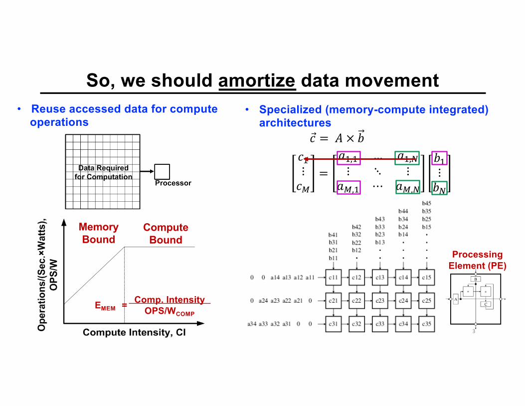
So, we should amortize data movement

EMEMComp. Intensity

OPS/WCOMP=

MemoryBound

ComputeBound

• Specialized (memory-compute integrated) architectures

!"⋮!$

=&"," … &",)⋮ ⋱ ⋮

&$," ⋯ &$,)

,"⋮,)

Processing Element (PE)

• Reuse accessed data for computeoperations

!⃗ = . × ,

3

In-memory computing (IMC)

IMC Mode SRAM Mode

!

"[J. Zhang, VLSI’16][J. Zhang, JSSC’17]

• In SRAM mode, matrix A stored in bit cells row-by-row

• In IMC mode, many WLs driven simultaneously→ amortize comm. cost inside array

• Can apply to diff. mem. Technologies→ enhanced scalability→ embedded non-volatility

#$⋮#&

=($,$ … ($,+⋮ ⋱ ⋮

(&,$ ⋯ (&,+

.$⋮.+

#⃗ = 0. ⇒

4

The basic tradeoffs

CONSIDER: Accessing ! bits of data associated with computation,from array with ! columns ⨉ ! rows.

Memory(D1/2×D1/2 array)

Computation

Memory &Computation(D1/2×D1/2 array)

D1/2

Traditional IMC Metric Traditional In-memoryBandwidth 1/D1/2 1Latency D 1Energy D3/2 ~DSNR 1 ~1/D1/2

• IMC benefits energy/delay at cost of SNR

• SNR-focused systems design is critical (circuits, architectures, algorithms)

5

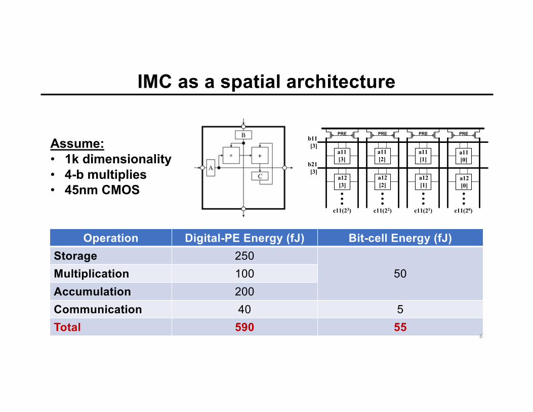
IMC as a spatial architecture

Operation Digital-PE Energy (fJ) Bit-cell Energy (fJ)Storage 250

50Multiplication 100Accumulation 200Communication 40 5Total 590 55

Assume:• 1k dimensionality• 4-b multiplies• 45nm CMOS

PRE

c11(23)

PRE PRE PRE

a11[3]

b11[3]

a11[2]

a11[1]

a11[0]

a12[3]

a12[2]

a12[1]

a12[0]

b21[3]

c11(22) c11(21) c11(20)

6

Where does IMC stand today?

Energy Efficiency (TOPS/W)

Norm

alize

d Th

roug

hput

(GOP

S/m

m2 )

Bankman, ISSCC’18, 28nm

Yuan, VLSI’18, 65nm

Moons, ISSCC’17, 28nmAndo, VLSI’17, 65nm

Chen, ISSCC’16, 65nm Gonug, ISSCC’18, 65nm

Biswas, ISSCC’18, 65nm

Jiang, VLSI’18, 65nm

10

10e2

10e3

10e4

Valavi, VLSI’18, 65nm

Khwa, ISSCC’18, 65nm

Zhang, VLSI’16, 130nm

Lee, ISSCC’18, 65nm

Shin, ISSCC’17, 65nm

Yin, VLSI’17, 65nm

10e-2 10e-1 1 10 10e2 10e3Energy Efficiency (TOPS/W)

On-c

hip

Mem

ory

Size

(kB)

Yuan, VLSI’18, 65nm

10e3

10e2

10

1

10e-2 10e-1 1 10 10e2 10e3

Valavi, VLSI’18, 65nm

Bankman, ISSCC’18, 28nm

Lee, ISSCC’18, 65nm

Zhang, VLSI’16, 130nm

Khwa, ISSCC’18, 65nm

Jiang, VLSI’18, 65nm

Biswas, ISSCC’18, 65nm

Gonug, ISSCC’18, 65nm

Chen, ISSCC’16, 65nm

Yin, VLSI’17, 65nm

Ando, VLSI’17, 65nm Moons, ISSCC’17, 28nm

IMCNot IMC

• Potential for 10× higher efficiency & throughput

• Limited scale, robustness, configurability

7

IMC challenge (1): analog computation• Need analog to ‘fit’ compute in bit cells (SNR limited by analog non-idealities)⟶ Must be feasible/competitive @ 16/12/7nm

Noise Limited Linearity/variation Limited

[R. Sarpeshkar, Ultra Low Power Bioelectronic]

0 1.20.4 0.8

0

20

40

60

80

WL Voltage (V)

Bit c

ell C

urre

nt ("

A)(10k-pt MC sim.)

8

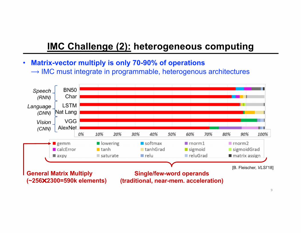
IMC Challenge (2): heterogeneous computing

[B. Fleischer, VLSI’18]General Matrix Multiply(~256⨉2300=590k elements)

Single/few-word operands(traditional, near-mem. acceleration)

• Matrix-vector multiply is only 70-90% of operations⟶ IMC must integrate in programmable, heterogenous architectures

9

IMC Challenge (3): efficient application mappings

• IMC engines must be ‘virtualized’⟶ IMC amortizes MVM costs, not weight loading. But…⟶ Need new mapping algorithms (physical tradeoffs very diff. than digital engines)

• EDRAM→IMC/4-bit: 40pJ• Reuse: "×$×% (10-20 lyrs)• EMAC,4-b: 50fJ

Activation Accessing Weight Accessing• EDRAM→IMC/4-bit: 40pJ• Reuse: &×'• EMAC,4-b:50fJ

Reuse ≈ 1k

MemoryBound

ComputeBound

10

Low-SNR computation via algorithmic co-design

[M. Verhelst, ISSCC SC on Machine Learning (2018)]

Data statistics

HW statistics

LEARNING MODELS &

PARMATER TRAININGALGORITHMS

Opportunity for top-down and bottom-up design

(courtesy IBM)

~75mm2 for 100M-parameter model(28nm)

11

Emerging non-volatile memory (NVM)

12

https://www.spinmemory.com/technologies/mram-overview/

MRAM/RRAM

(nonvolatility)

• 2-terminal resistive memory provides better scaling at advanced nodes

• … BUT, leads to significantly reduced SNR

Globalfoundries, 22nm [D. Shum, VLSI’17]

Signal

Noise

Magnetic RAM (MRAM)

Resistive RAM (RRAM)

TSMC 16nm [H. W. Pan, IEDM’15]

Chip-specific parameter trainingEx.: MNIST Classification with Binarized NN(implemented on chip)

[J. Zhang, IEEE JETCAS’19]

Update parameters based on errors

Determine errors

Chip-generalized parameter training • HW-generalized Stochastic Training

• HW-specific Inference

gi (hardware sample)

Model Parameters#(%, ', ℒ)

G(hardware statistics)

(Chipspecific)

(Chipgeneralized)

ℒ,-./

[B. Zhang, ICASSP 2019]

CIFAR-10 Classification using Binarized NN(simulated)

Statistical model in PyTorch,

Keras

High-SNR, charge-domain IMC

15[H. Valavi, VLSI’18] [H. Valavi, JSSC’19]

W1,1,1n

W1,1,1n

IA1,1,1

IA1,2,1

8T Multiplying Bit Cell (M-BC)1. Digital multiplication2. Analog accumulation

Two modes: o XNOR: !",$,%& = ()",$,% ⊕+,,-,%

&

o AND: !",$,%& = ()",$,% ×+,,-,%&

(i.e., keep ()",$,% high)

WLWL IAbx,y,z

Wbi,j,zn Wi,j,zn

BL

Ox,y,zn

IAx,y,z

BLb

Pre-activation PAn

(Image: SILVACO)

Wires

Capacitor

M-BC Transistors

(approx. 80% area overhead compared to standard 6T bit cell)

• Capacitors provide much better controllability & technology scalability⟶ 10’s of thousands of IMC rows before SNR is capacitor limited

2.4Mb, 64-tile IMC

Moons,ISSCC’17

Bang,ISSCC’17

Ando,VLSI’17

Bankman,ISSCC’18

Valavi, VLSI’18

Technology 28nm 40nm 65nm 28nm 65nm

Area (!!") 1.87 7.1 12 6 17.6

Operating VDD 1 0.63-0.9 0.55-1 0.8/0.8 (0.6/0.5) 0.94/0.68/1.2

Bit precision 4-16b 6-32b 1b 1b 1b

on-chip Mem. 128kB 270kB 100kB 328kB 295kB

Throughput (GOPS) 400 108 1264 400 (60) 18,876

TOPS/W 10 0.384 6 532 (772) 866

• 10-layer CNN demos for MNIST/CIFAR-10/SVHN at energies of 0.8/3.55/3.55 μJ/image

• Equivalent performance to software implementation

[H. Valavi, VLSI’18]16

Programmable heterogeneous IMC processor

CPU(RISC-V)

AXI Bus

DMA Timers GPIO UART

32

Program Memory(128 kB)

Boot-loader

Data Memory(128 kB)

Compute-In-Memory Unit (CIMU)

• 590 kb • 16 bank

Ext. Mem. I/F

Config.Regs.

To E2PROM To DRAM Controller

Config

APB Bus 32

32

Tx Rx

8 13(data) (addr.)

32(data/addr.)

ADC

& AB

N

w2b

Res

hapi

ng B

uffe

r

Inpu

t-Vec

tor G

ener

ator

x

Row

Dec

oder

/ WL

Driv

ers

Memory Read/Write I/F

32b

8b

Near-Mem. Data Path

32b

ADC

& AB

N

A32b

Bit Cell

Compute-In-Memory Array

(CIMA)

f(y = A x)

1. Interfaces to standard processor memory space2. Digital near-mem. accelerator (element compute)3. Bit scalability from 1 to 8 bits

[H. Jia, arXiv:1811.04047] [H. Jia, HotChips’19]

Bit-Parallel/Bit-Serial (BP/BS) Multi-bit IMC

10

203040

6

10

14

18

2 3 4 5 6 7 8

2

4

6

BA

SQNR

(dB)

Bx=2

Bx=4

Bx=8

N=2304, 2000, 1500, 1000, 500, 255

N=2304, 2000, 1500, 1000, 500, 255

N=2304, 2000, 1500, 1000, 500, 255

• SQNR different that standard INT compute- rounding effects are well modeled- SQNR is high at precisions of interest

8-b SAR ADC(15|18% energy|areaoverhead)

1 1 0 1 0 0

ADC

8b

Max. Dynamic Range: 2304

Dynamic Range: 256

x0[Bx-1:0] : 0-1-0

a0,0 a1,0

xN-1[Bx-1:0] : 0-0-0

x2303[Bx-1:0] : 1-1-0

[BA-1:0] [BA-1:0](E.g., BA=3, Bx=3)

5

Development board

To Host Processor

19

Software libraries1. Deep-learning Training Libraries

(Keras)2. Deep-learning Inference Libraries

(Python, MATLAB, C)

Dense(units, ...)Conv2D(filters, kernel_size, ...)...

Standard Keras libs:

QuantizedDense(units, nb_input=4, nb_weight=4, chip_quant=True, ...)

QuantizedConv2D(filters, kernel_size, nb_input=4, nb_weight=4, chip_quant=True, ...)

...

QuantizedDense(units, nb_input=4, nb_weight=4, chip_quant=False, ...)

QuantizedConv2D(filters, kernel_size, nb_input=4, nb_weight=4, chip_quant=False, ...)

...

Custom libs:(INT/CHIP quant.)

chip_mode = Trueoutputs = QuantizedConv2D(inputs,

weights, biases, layer_params)outputs = BatchNormalization(inputs,

layer_params)...

High-level network build (Python):

Embedded C:

Function calls to chip (Python):chip.load_config(num_tiles, nb_input=4,

nb_weight=4)chip.load_weights(weights2load)chip.load_image(image2load)outputs = chip.image_filter()

chip_command = get_uart_word();chip_config(); load_weights(); load_image();image_filter(chip_command);read_dotprod_result(image_filter_command);20

Demonstrations

2 4 6 82

4

6

8

2 4 6 85

10

15

20

SQNR

(dB)

Multi-bit Matrix-Vector Multiplication

N=1152Bit-true Sim.

N=1728

MeasuredN=1152N=1728

Bx=2

BA

Bx=4

0 20 40 60 80-500

0

500

0 20 40 60 80-60

-40

-20

0

20

Data Index

Com

pute

Val

ue

Bx=2, BA=2 Bx=4, BA=4

Bit True Sim.Measured

BA

Data Index

Neural-Network DemonstrationsNetwork A

(4/4-b activations/weights)Network B

(1/1-b activations/weights)Accuracy of chip

(vs. ideal)92.4%

(vs. 92.7%)89.3%

(vs. 89.8%)Energy/10-way

Class.1 105.2 μJ 5.31 μJ

Throughput1 23 images/sec. 176 images/sec.

Neural Network Topology

L1: 128 CONV3 – Batch normL2: 128 CONV3 – POOL – Batch norm.L3: 256 CONV3 – Batch. normL4: 256 CONV3 – POOL – Batch norm.L5: 256 CONV3 – Batch norm.L6: 256 CONV3 – POOL – Batch norm.L7-8: 1024 FC – Batch norm.L9: 10 FC – Batch norm.

L1: 128 CONV3 – Batch Norm.L2: 128 CONV3 – POOL – Batch Norm.L3: 256 CONV3 – Batch Norm.L4: 256 CONV3 – POOL – Batch Norm.L5: 256 CONV3 – Batch Norm.L6: 256 CONV3 – POOL – Batch Norm.L7-8: 1024 FC – Batch norm.L9: 10 FC – Batch norm.

DM

EM

PM

EM

CP

U

CIMU

AD

C

AB

N

DM

A e

tc. W2b Reshaping Buffer

4×4CIMATiles

3mm

4.5mm

Nea

r-m

em. D

atap

ath

Sparsity Controller

[H. Jia, arXiv:1811.04047]21

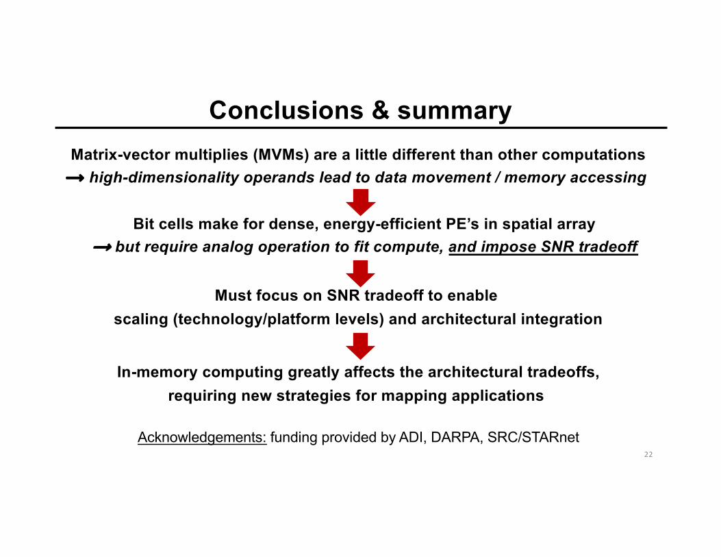
Conclusions & summaryMatrix-vector multiplies (MVMs) are a little different than other computations⟶ high-dimensionality operands lead to data movement / memory accessing

Bit cells make for dense, energy-efficient PE’s in spatial array⟶ but require analog operation to fit compute, and impose SNR tradeoff

Must focus on SNR tradeoff to enable scaling (technology/platform levels) and architectural integration

In-memory computing greatly affects the architectural tradeoffs,requiring new strategies for mapping applications

Acknowledgements: funding provided by ADI, DARPA, SRC/STARnet22