advanced user guide - sciex · report templates ... this advanced user guide provides information...
TRANSCRIPT

Analyst® 1.6.1 Software
Advanced User Guide
Release Date: March 2012

This document is provided to customers who have purchased AB Sciex equipment to use in the operation of such AB Sciex equipment. This document is copyright protected and any reproduction of this document or any part of this document is strictly prohibited, except as AB Sciex may authorize in writing.
Software that may be described in this document is furnished under a license agreement. It is against the law to copy, modify, or distribute the software on any medium, except as specifically allowed in the license agreement. Furthermore, the license agreement may prohibit the software from being disassembled, reverse engineered, or decompiled for any purpose.
Portions of this document may make reference to other manufacturers and/or their products, which may contain parts whose names are registered as trademarks and/or function as trademarks of their respective owners. Any such use is intended only to designate those manufacturers' products as supplied by AB Sciex for incorporation into its equipment and does not imply any right and/or license to use or permit others to use such manufacturers' and/or their product names as trademarks.
AB Sciex makes no warranties or representations as to the fitness of this equipment for any particular purpose and assumes no responsibility or contingent liability, including indirect or consequential damages, for any use to which the purchaser may put the equipment described herein, or for any adverse circumstances arising therefrom.
For research use only. Not for use in diagnostic procedures.
The trademarks mentioned herein are the property of AB Sciex Pte. Ltd. or their respective owners.AB SCIEX™ is being used under license.
AB SCIEX71 Four Valley Dr., Concord, Ontario, Canada. L4K 4V8.AB Sciex LP is ISO 9001 registered.© 2012 AB SCIEX.Printed in Canada.

Contents
Foreword. . . . . . . . . . . . . . . . . . . . . . . . . . . . . . . . . . . . . . . . . . . . . . . . . . . . . . . . . . 7
Access System Documentation . . . . . . . . . . . . . . . . . . . . . . . . . . . . . . . . . . . . . .7Contact Technical Support . . . . . . . . . . . . . . . . . . . . . . . . . . . . . . . . . . . . . . . . . .7
Chapter 1 General Information . . . . . . . . . . . . . . . . . . . . . . . . . . . . . . . . . . . . . . . . 9
Analyst Service . . . . . . . . . . . . . . . . . . . . . . . . . . . . . . . . . . . . . . . . . . . . . . . . . . .9API Instrument Project Folders . . . . . . . . . . . . . . . . . . . . . . . . . . . . . . . . . . . . . .10Program Files . . . . . . . . . . . . . . . . . . . . . . . . . . . . . . . . . . . . . . . . . . . . . . . . . . .10Projects and Subprojects . . . . . . . . . . . . . . . . . . . . . . . . . . . . . . . . . . . . . . . . . .11
Subprojects . . . . . . . . . . . . . . . . . . . . . . . . . . . . . . . . . . . . . . . . . . . . . . . . . . .11Project Organization . . . . . . . . . . . . . . . . . . . . . . . . . . . . . . . . . . . . . . . . . . . .12
Software Security . . . . . . . . . . . . . . . . . . . . . . . . . . . . . . . . . . . . . . . . . . . . . . . .13Workspaces . . . . . . . . . . . . . . . . . . . . . . . . . . . . . . . . . . . . . . . . . . . . . . . . . . . .13
Chapter 2 Instrument Tuning and Calibration. . . . . . . . . . . . . . . . . . . . . . . . . . . 15
Automatic Tuning and Calibration . . . . . . . . . . . . . . . . . . . . . . . . . . . . . . . . . . . .15Back up Instrument Parameters . . . . . . . . . . . . . . . . . . . . . . . . . . . . . . . . . . .16Restore Instrument Parameters . . . . . . . . . . . . . . . . . . . . . . . . . . . . . . . . . . .16
Compound Optimization . . . . . . . . . . . . . . . . . . . . . . . . . . . . . . . . . . . . . . . . . . .16Flow Injection Analysis . . . . . . . . . . . . . . . . . . . . . . . . . . . . . . . . . . . . . . . . . . . .16Infusion . . . . . . . . . . . . . . . . . . . . . . . . . . . . . . . . . . . . . . . . . . . . . . . . . . . . . . . .17
Chapter 3 Batches . . . . . . . . . . . . . . . . . . . . . . . . . . . . . . . . . . . . . . . . . . . . . . . . . 19
Batch Editor . . . . . . . . . . . . . . . . . . . . . . . . . . . . . . . . . . . . . . . . . . . . . . . . . . . . .19Batch Files . . . . . . . . . . . . . . . . . . . . . . . . . . . . . . . . . . . . . . . . . . . . . . . . . . . . .20
Build a Batch as a Text File . . . . . . . . . . . . . . . . . . . . . . . . . . . . . . . . . . . . . . .20Import a Batch as a Text File . . . . . . . . . . . . . . . . . . . . . . . . . . . . . . . . . . . . . .20Set Quantitation Details in the Batch Editor (Optional) . . . . . . . . . . . . . . . . . .21
Chapter 4 Device Methods . . . . . . . . . . . . . . . . . . . . . . . . . . . . . . . . . . . . . . . . . . 23
Devices in Acquisition Methods . . . . . . . . . . . . . . . . . . . . . . . . . . . . . . . . . . . . .23Add or Remove an LC Device . . . . . . . . . . . . . . . . . . . . . . . . . . . . . . . . . . . . .23Set the LC Pump Properties . . . . . . . . . . . . . . . . . . . . . . . . . . . . . . . . . . . . . .24Set the Autosampler Properties . . . . . . . . . . . . . . . . . . . . . . . . . . . . . . . . . . . .24Set the Column Oven Properties . . . . . . . . . . . . . . . . . . . . . . . . . . . . . . . . . . .24Set the Switching Valve Properties . . . . . . . . . . . . . . . . . . . . . . . . . . . . . . . . .25Set the Diode Array Detector Parameters . . . . . . . . . . . . . . . . . . . . . . . . . . . .25Set the Analog-to-Digital Converter Properties . . . . . . . . . . . . . . . . . . . . . . . .25
Dynamic Fill Time . . . . . . . . . . . . . . . . . . . . . . . . . . . . . . . . . . . . . . . . . . . . . . . .27Experiments and Periods . . . . . . . . . . . . . . . . . . . . . . . . . . . . . . . . . . . . . . . . . .27
Experiments . . . . . . . . . . . . . . . . . . . . . . . . . . . . . . . . . . . . . . . . . . . . . . . . . . .27Periods . . . . . . . . . . . . . . . . . . . . . . . . . . . . . . . . . . . . . . . . . . . . . . . . . . . . . .27
Information Dependent Acquisition Methods . . . . . . . . . . . . . . . . . . . . . . . . . . .28Solvent Compressibility Values . . . . . . . . . . . . . . . . . . . . . . . . . . . . . . . . . . . . . .29Syringe Size Versus Flow Rate . . . . . . . . . . . . . . . . . . . . . . . . . . . . . . . . . . . . . .29
Advanced User Guide
Release Date: March 2012Analyst® 1.6.1 Software
3 of 94

Chapter 5 Qualitative Data Analysis . . . . . . . . . . . . . . . . . . . . . . . . . . . . . . . . . . 31
Chromatograms . . . . . . . . . . . . . . . . . . . . . . . . . . . . . . . . . . . . . . . . . . . . . . . . .31Spectra . . . . . . . . . . . . . . . . . . . . . . . . . . . . . . . . . . . . . . . . . . . . . . . . . . . . . . . .32Background Subtraction . . . . . . . . . . . . . . . . . . . . . . . . . . . . . . . . . . . . . . . . . . .32
Perform a Background Subtraction from a Spectrum . . . . . . . . . . . . . . . . . . .32Unlock the Ranges . . . . . . . . . . . . . . . . . . . . . . . . . . . . . . . . . . . . . . . . . . . . .33
Background Subtract to File . . . . . . . . . . . . . . . . . . . . . . . . . . . . . . . . . . . . . . . .33Perform a Background Subtraction to File . . . . . . . . . . . . . . . . . . . . . . . . . . . .33
Baseline Subtract . . . . . . . . . . . . . . . . . . . . . . . . . . . . . . . . . . . . . . . . . . . . . . . .34Calculators . . . . . . . . . . . . . . . . . . . . . . . . . . . . . . . . . . . . . . . . . . . . . . . . . . . . .35
Elemental Composition Calculator . . . . . . . . . . . . . . . . . . . . . . . . . . . . . . . . .35Hypermass Calculator . . . . . . . . . . . . . . . . . . . . . . . . . . . . . . . . . . . . . . . . . . .35Elemental Targeting Calculator . . . . . . . . . . . . . . . . . . . . . . . . . . . . . . . . . . . .35Mass Property Calculator . . . . . . . . . . . . . . . . . . . . . . . . . . . . . . . . . . . . . . . .36Isotopic Distribution Calculator . . . . . . . . . . . . . . . . . . . . . . . . . . . . . . . . . . . .36Centroided Peaks . . . . . . . . . . . . . . . . . . . . . . . . . . . . . . . . . . . . . . . . . . . . . .36Calculate the Centroid of a Peak . . . . . . . . . . . . . . . . . . . . . . . . . . . . . . . . . . .36
Data Analysis . . . . . . . . . . . . . . . . . . . . . . . . . . . . . . . . . . . . . . . . . . . . . . . . . . .37Total Ion Chromatogram . . . . . . . . . . . . . . . . . . . . . . . . . . . . . . . . . . . . . . . . .37Extracted Ion Chromatogram . . . . . . . . . . . . . . . . . . . . . . . . . . . . . . . . . . . . .37Base Peak Chromatogram . . . . . . . . . . . . . . . . . . . . . . . . . . . . . . . . . . . . . . .37Extracted Wavelength Chromatogram . . . . . . . . . . . . . . . . . . . . . . . . . . . . . .38Diode Array Detector . . . . . . . . . . . . . . . . . . . . . . . . . . . . . . . . . . . . . . . . . . . .38Total Wavelength Chromatogram . . . . . . . . . . . . . . . . . . . . . . . . . . . . . . . . . .38Overlay Graphs . . . . . . . . . . . . . . . . . . . . . . . . . . . . . . . . . . . . . . . . . . . . . . . .38Cycle Between Overlaid Graphs . . . . . . . . . . . . . . . . . . . . . . . . . . . . . . . . . . .39Sum Overlays . . . . . . . . . . . . . . . . . . . . . . . . . . . . . . . . . . . . . . . . . . . . . . . . .39
Graphs Labels . . . . . . . . . . . . . . . . . . . . . . . . . . . . . . . . . . . . . . . . . . . . . . . . . . .39Add Captions to a Graph . . . . . . . . . . . . . . . . . . . . . . . . . . . . . . . . . . . . . . . . .39Add Text to a Graph . . . . . . . . . . . . . . . . . . . . . . . . . . . . . . . . . . . . . . . . . . . .40
Compound Database . . . . . . . . . . . . . . . . . . . . . . . . . . . . . . . . . . . . . . . . . . . . .40Contour Plots . . . . . . . . . . . . . . . . . . . . . . . . . . . . . . . . . . . . . . . . . . . . . . . . . . .40
View a Contour Plot . . . . . . . . . . . . . . . . . . . . . . . . . . . . . . . . . . . . . . . . . . . . .41Select an Area in a Contour Plot . . . . . . . . . . . . . . . . . . . . . . . . . . . . . . . . . . .41Set the Intensity and Absorbance in a Contour Plot . . . . . . . . . . . . . . . . . . . .42Change Colors in a Contour Plot . . . . . . . . . . . . . . . . . . . . . . . . . . . . . . . . . . .42
Dynamic Background Subtraction Algorithm . . . . . . . . . . . . . . . . . . . . . . . . . . . .42Fragment Interpretation . . . . . . . . . . . . . . . . . . . . . . . . . . . . . . . . . . . . . . . . . . . .42Connect the Fragment Interpretation Tool to a Spectrum . . . . . . . . . . . . . . . . . .43
Match Fragments with Peaks . . . . . . . . . . . . . . . . . . . . . . . . . . . . . . . . . . . . .44Select a Bond in a Molecular Structure . . . . . . . . . . . . . . . . . . . . . . . . . . . . . .44View Isotopes . . . . . . . . . . . . . . . . . . . . . . . . . . . . . . . . . . . . . . . . . . . . . . . . .44Display a Formula Difference in a Spectrum . . . . . . . . . . . . . . . . . . . . . . . . . .44Display a Formula Difference in the Fragment List . . . . . . . . . . . . . . . . . . . . .45Display a Formula Difference in a Molecular Structure . . . . . . . . . . . . . . . . . .45
IDA Explorer . . . . . . . . . . . . . . . . . . . . . . . . . . . . . . . . . . . . . . . . . . . . . . . . . . . .45Library Databases . . . . . . . . . . . . . . . . . . . . . . . . . . . . . . . . . . . . . . . . . . . . . . . .46
Switch Between Existing Library Databases . . . . . . . . . . . . . . . . . . . . . . . . . .47Connect to a Local Library Database . . . . . . . . . . . . . . . . . . . . . . . . . . . . . . .48
Analyst® 1.6.1 Software
4 of 94
Advanced User Guide
Release Date: March 2012

Connect to a Server Library Database . . . . . . . . . . . . . . . . . . . . . . . . . . . . . .48View All Library Records . . . . . . . . . . . . . . . . . . . . . . . . . . . . . . . . . . . . . . . . .49Add a Record to the Library . . . . . . . . . . . . . . . . . . . . . . . . . . . . . . . . . . . . . . .49Search Library Records with Constraints . . . . . . . . . . . . . . . . . . . . . . . . . . . .50Library Search Tips . . . . . . . . . . . . . . . . . . . . . . . . . . . . . . . . . . . . . . . . . . . . .51Search for a Similar Spectrum . . . . . . . . . . . . . . . . . . . . . . . . . . . . . . . . . . . . .51View a Compound from the Search Results . . . . . . . . . . . . . . . . . . . . . . . . . .53
Processed Data Files . . . . . . . . . . . . . . . . . . . . . . . . . . . . . . . . . . . . . . . . . . . . .53Save a Processed Data File . . . . . . . . . . . . . . . . . . . . . . . . . . . . . . . . . . . . . .53Open a Processed Data File . . . . . . . . . . . . . . . . . . . . . . . . . . . . . . . . . . . . . .53
Qualitative Data . . . . . . . . . . . . . . . . . . . . . . . . . . . . . . . . . . . . . . . . . . . . . . . . . .53Signal-to-Noise Ratio . . . . . . . . . . . . . . . . . . . . . . . . . . . . . . . . . . . . . . . . . . . . .54Smoothing Algorithms . . . . . . . . . . . . . . . . . . . . . . . . . . . . . . . . . . . . . . . . . . . . .54
Smooth Data using the Smooth Algorithm . . . . . . . . . . . . . . . . . . . . . . . . . . .55Smooth Data using Gaussian Smoothing . . . . . . . . . . . . . . . . . . . . . . . . . . . .55
Spectral Arithmetic Wizard . . . . . . . . . . . . . . . . . . . . . . . . . . . . . . . . . . . . . . . . .56Toolbar Icons . . . . . . . . . . . . . . . . . . . . . . . . . . . . . . . . . . . . . . . . . . . . . . . . . . .56
Chapter 6 Quantitative Data Analysis . . . . . . . . . . . . . . . . . . . . . . . . . . . . . . . . . 59
Calibration Options . . . . . . . . . . . . . . . . . . . . . . . . . . . . . . . . . . . . . . . . . . . . . . .59About Calibration Curves . . . . . . . . . . . . . . . . . . . . . . . . . . . . . . . . . . . . . . . . .59Select the Best Regression Type . . . . . . . . . . . . . . . . . . . . . . . . . . . . . . . . . .59
Integration Algorithms . . . . . . . . . . . . . . . . . . . . . . . . . . . . . . . . . . . . . . . . . . . . .60Analyst Classic and IntelliQuan Integration Algorithms . . . . . . . . . . . . . . . . . .61
Quantitation Method-Creation Tools . . . . . . . . . . . . . . . . . . . . . . . . . . . . . . . . . .62Wizards . . . . . . . . . . . . . . . . . . . . . . . . . . . . . . . . . . . . . . . . . . . . . . . . . . . . . .62Find Peaks Using an Automatic Method . . . . . . . . . . . . . . . . . . . . . . . . . . . . .63Quantitation Method Editor . . . . . . . . . . . . . . . . . . . . . . . . . . . . . . . . . . . . . . .63The Semi-Automatic Method Editor . . . . . . . . . . . . . . . . . . . . . . . . . . . . . . . . .63Find Peaks Using a Semi-Automatic Method . . . . . . . . . . . . . . . . . . . . . . . . .64
Metric Plots . . . . . . . . . . . . . . . . . . . . . . . . . . . . . . . . . . . . . . . . . . . . . . . . . . . . .64Generate a Metric Temporary Plot . . . . . . . . . . . . . . . . . . . . . . . . . . . . . . . . .65Generate a Metric Plot and Save the Plot Criteria . . . . . . . . . . . . . . . . . . . . . .65Save Default Plot Criteria for Future Results Tables . . . . . . . . . . . . . . . . . . . .67
Noise and Area Threshold Parameters . . . . . . . . . . . . . . . . . . . . . . . . . . . . . . . .67Recalculate the Noise and Area Threshold . . . . . . . . . . . . . . . . . . . . . . . . . . .68
Peak Integration . . . . . . . . . . . . . . . . . . . . . . . . . . . . . . . . . . . . . . . . . . . . . . . . .68Peak Review . . . . . . . . . . . . . . . . . . . . . . . . . . . . . . . . . . . . . . . . . . . . . . . . . . . .68
Peak Review Tips . . . . . . . . . . . . . . . . . . . . . . . . . . . . . . . . . . . . . . . . . . . . . .69Detect Peaks . . . . . . . . . . . . . . . . . . . . . . . . . . . . . . . . . . . . . . . . . . . . . . . . . .69Find the Potential Peak Start . . . . . . . . . . . . . . . . . . . . . . . . . . . . . . . . . . . . . .70Confirm the Peak Start . . . . . . . . . . . . . . . . . . . . . . . . . . . . . . . . . . . . . . . . . .70Find the Peak Top . . . . . . . . . . . . . . . . . . . . . . . . . . . . . . . . . . . . . . . . . . . . . .71Find the Peak End . . . . . . . . . . . . . . . . . . . . . . . . . . . . . . . . . . . . . . . . . . . . . .73Separate Peaks . . . . . . . . . . . . . . . . . . . . . . . . . . . . . . . . . . . . . . . . . . . . . . . .74
Queries . . . . . . . . . . . . . . . . . . . . . . . . . . . . . . . . . . . . . . . . . . . . . . . . . . . . . . . .75Queries on Sample Type . . . . . . . . . . . . . . . . . . . . . . . . . . . . . . . . . . . . . . . . .75Default Queries and Table-Specific Queries . . . . . . . . . . . . . . . . . . . . . . . . . .75How Accuracy Variations Affect the Results . . . . . . . . . . . . . . . . . . . . . . . . . .76
Regression . . . . . . . . . . . . . . . . . . . . . . . . . . . . . . . . . . . . . . . . . . . . . . . . . . . . .76
Advanced User Guide
Release Date: March 2012Analyst® 1.6.1 Software
5 of 94

Linear Regression . . . . . . . . . . . . . . . . . . . . . . . . . . . . . . . . . . . . . . . . . . . . . .77Linear Through Zero Regression . . . . . . . . . . . . . . . . . . . . . . . . . . . . . . . . . . .77Mean Response Factor . . . . . . . . . . . . . . . . . . . . . . . . . . . . . . . . . . . . . . . . . .77Power . . . . . . . . . . . . . . . . . . . . . . . . . . . . . . . . . . . . . . . . . . . . . . . . . . . . . . .78Quadratic Calibration Equation . . . . . . . . . . . . . . . . . . . . . . . . . . . . . . . . . . . .78
Report Templates . . . . . . . . . . . . . . . . . . . . . . . . . . . . . . . . . . . . . . . . . . . . . . . .79Customize Reports . . . . . . . . . . . . . . . . . . . . . . . . . . . . . . . . . . . . . . . . . . . . .81Preview, Print, and Export Reports . . . . . . . . . . . . . . . . . . . . . . . . . . . . . . . . .81
Results Tables . . . . . . . . . . . . . . . . . . . . . . . . . . . . . . . . . . . . . . . . . . . . . . . . . .82Define the Layout of Results Tables . . . . . . . . . . . . . . . . . . . . . . . . . . . . . . . .82Sort Data in Results Tables . . . . . . . . . . . . . . . . . . . . . . . . . . . . . . . . . . . . . . .83Sort a Results Table and Save the Sort Criteria . . . . . . . . . . . . . . . . . . . . . . .83Save Default Sort Criteria for Future Results Tables . . . . . . . . . . . . . . . . . . .84Sort a Results Table using Preset Sort Criteria . . . . . . . . . . . . . . . . . . . . . . . .85About using Queries with Results Tables . . . . . . . . . . . . . . . . . . . . . . . . . . . .85Compare Results Between Batches . . . . . . . . . . . . . . . . . . . . . . . . . . . . . . . .85How Concentration Levels Affect Results . . . . . . . . . . . . . . . . . . . . . . . . . . . .86Results Table Layouts . . . . . . . . . . . . . . . . . . . . . . . . . . . . . . . . . . . . . . . . . . .86Summary Layout View . . . . . . . . . . . . . . . . . . . . . . . . . . . . . . . . . . . . . . . . . . .87Analyte Layout View . . . . . . . . . . . . . . . . . . . . . . . . . . . . . . . . . . . . . . . . . . . .87Analyte Group Layout View . . . . . . . . . . . . . . . . . . . . . . . . . . . . . . . . . . . . . . .88Results Table Fields . . . . . . . . . . . . . . . . . . . . . . . . . . . . . . . . . . . . . . . . . . . .88
Results Table Tips . . . . . . . . . . . . . . . . . . . . . . . . . . . . . . . . . . . . . . . . . . . . . . .94Weighting Factors . . . . . . . . . . . . . . . . . . . . . . . . . . . . . . . . . . . . . . . . . . . . . . . .94
Analyst® 1.6.1 Software
6 of 94
Advanced User Guide
Release Date: March 2012

Foreword
This Advanced User Guide provides information about the Analyst® software features.
Access System DocumentationThe Help, guides, and tutorials for the instrument and the software are installed automatically.
• Click Start > All Programs > AB SCIEX > Analyst. A complete list of the available documentation can be found in the Help.
• Press F1 to open the Help.
Contact Technical SupportThe manufacturer and its representatives maintain a staff of fully-trained service and technical specialists located throughout the world. They can answer questions about the instrument or any technical issues that may arise. For more information, visit the Web site at www.absciex.com or contact Technical Support using [email protected].
Advanced User Guide
Release Date: March 2012Analyst® 1.6.1 Software
7 of 94

Analyst® 1.6.1 Software
8 of 94
Advanced User Guide
Release Date: March 2012

1
General InformationThe software is divided into discrete functional areas called modes. Modes allow the user to perform activities related to a main task. Modes are accessed through the Navigation bar or the Mode list in the toolbar. Users can switch from one mode to another without any loss of work. For more information, refer to the Analyst® software Show Me tutorial.
Analyst ServiceThe Analyst Service is the communication path between the instrument and attached devices. The Analyst Service is started each time the Analyst software is started. In general the Analyst Service starts automatically when the user logs on to Windows. If the service is not running when the Analyst software is started, then the Analyst Service will start automatically.
Figure 1-1 Analyst Software Window
Item Description1 Mode list
2 Navigation bar
1
2
Advanced User Guide
Release Date: March 2012Analyst® 1.6.1 Software
9 of 94
General Information
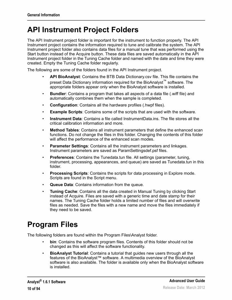
API Instrument Project FoldersThe API Instrument project folder is important for the instrument to function properly. The API Instrument project contains the information required to tune and calibrate the system. The API Instrument project folder also contains data files for a manual tune that was performed using the Start button instead of the Acquire button. These data files are saved automatically in the API Instrument project folder in the Tuning Cache folder and named with the date and time they were created. Empty the Tuning Cache folder regularly.
The following are some of the folders found in the API Instrument project.
• API BioAnalyst: Contains the BTB Data Dictionary.csv file. This file contains the preset Data Dictionary information required for the BioAnalyst™ software. The appropriate folders appear only when the BioAnalyst software is installed.
• Bundler: Contains a program that takes all aspects of a data file (.wiff file) and automatically combines them when the sample is completed.
• Configuration: Contains all the hardware profiles (.hwpf files).
• Example Scripts: Contains some of the scripts that are used with the software.
• Instrument Data: Contains a file called InstrumentData.ins. The file stores all the critical calibration information and more.
• Method Tables: Contains all instrument parameters that define the enhanced scan functions. Do not change the files in this folder. Changing the contents of this folder will affect the performance of the enhanced scan modes.
• Parameter Settings: Contains all the instrument parameters and linkages. Instrument parameters are saved as ParamSettingsdef.psf files.
• Preferences: Contains the Tunedata.tun file. All settings (parameter, tuning, instrument, processing, appearances, and queue) are saved as Tunedata.tun in this folder.
• Processing Scripts: Contains the scripts for data processing in Explore mode. Scripts are found in the Script menu.
• Queue Data: Contains information from the queue.
• Tuning Cache: Contains all the data created in Manual Tuning by clicking Start instead of Acquire. Files are saved with a generic time and date stamp for their names. The Tuning Cache folder holds a limited number of files and will overwrite files as needed. Save the files with a new name and move the files immediately if they need to be saved.
Program FilesThe following folders are found within the Program Files\Analyst folder.
• bin: Contains the software program files. Contents of this folder should not be changed as this will affect the software functionality.
• BioAnalyst Tutorial: Contains a tutorial that guides new users through all the features of the BioAnalyst™ software. A multimedia overview of the BioAnalyst software is also available. The folder is available only when the BioAnalyst software is installed.
Analyst® 1.6.1 Software
10 of 94
Advanced User Guide
Release Date: March 2012

General Information
• Firmware: Contains the instrument system controller software (scu21.exe) and the instrument firmware files. Use these files to download new firmware to the instrument when required. For more information, refer to the software installation guide included with the software.
• Help: Contains the help files, guides, tutorials, release notes and software installation guide.
• Scripts: Contains all the scripts that can be installed. Research-grade scripts are available to extend the functionality of the software. Some scripts are installed automatically and some scripts can be installed individually. For more information, refer to the Scripts User Guide.
• Simulation: Contains the instrument data files required to run the software in simulation mode.
Projects and SubprojectsDecide where to store the files related to the experiment before starting the experiment. Use projects and subprojects for each experiment to manage the data better and compare the results.
SubprojectsA subproject contains a subset of the folders in the project. All subprojects must contain the same folders. Subprojects are useful for organizing data.
For example, if samples of various compounds from different laboratories are run using the same acquisition method, then create subprojects to store the results for each laboratory, but leave the acquisition method folder in the project. The acquisition method is then available for use in the subproject or laboratory. Alternatively, if samples are being analyzed over a period of several weeks, then the results from each day can be stored in a separate subproject. Refer to Figure 1-2 Example of a project and subproject folder structure.
Advanced User Guide
Release Date: March 2012Analyst® 1.6.1 Software
11 of 94

General Information
Figure 1-2 Example of a project and subproject folder structure
Project OrganizationA project is a folder structure for organizing and storing sample information, data, quantitation information and so forth. Within each project there are folders that can contain different types of files; for example, the Data folder contains acquisition data files. Table 1-1 describes the contents of the different folders.
The software can access a project only if it is stored in a root folder. Users cannot create projects in a folder that has not been defined as a root folder.
The preset root folder is Analyst Data on the drive where the software is installed. To store projects in other locations, create new root folders. For more information about root folders, refer to the Help.
Table 1-1 Project Folders
Folder Contents\Acquisition Methods Contains all acquisition methods used. Acquisition methods have the
.dam extension.
\Acquisition Scripts Contains all the acquisition batch scripts available.
\Batch Contains all the acquisition batch files used. Acquisition batches have the .dab extension. It also contains a subfolder, Templates, that contains acquisition batch templates. Batch templates have the .dat extension.
Analyst® 1.6.1 Software
12 of 94
Advanced User Guide
Release Date: March 2012

General Information
Software SecurityThe software has a number of functions for configuring and managing security. The Analyst® software administrator can:
• Choose a security mode to best suit the needs of the operating environment.
• Add and delete users and roles.
• Set access rights to users and roles as required.
• Control access to remote instrument stations.
• Control access to project files.
For more information about Analyst software security, refer to the Laboratory Director’s Guide.
WorkspacesA workspace is a particular arrangement of windows and panes, including any associated file or files. For example, while working on a particular data set, users can open and size various windows to help with the analysis. This arrangement, or workspace, can be saved so that the next time users look at the data, the window arrangement is identical.
In Quantitate and Explore modes, users can have multiple workspaces per session. This means that different workspaces can be designed to suit different tasks within these modes, and then save them for future use. When in one of these two modes, a particular workspace can be opened without exiting that mode.
\BioAnalyst Contains files used with the BioAnalyst™ software add-on, a protein analysis tool. The folder is available only when the BioAnalyst software is installed.
\Data Contains the acquisition data files (.wiff extension).
\Log Contains results of quantitation and compound optimization.
\Processing Methods Contains all qualitative data processing methods used.
\Processing Scripts Contains all data processing scripts available. Processing scripts stored in the API Instrument project appear in the Scripts menu.
\Project Information Contains all project information and settings for the project. This folder cannot be stored in a subproject.
\Quantitation Methods Contains all quantitation methods used. Quantitation methods have a .qmf extension.
\Results Contains all quantitation results table files (.rdb extension).
\Templates Contains report templates (.rpt extension).
Table 1-1 Project Folders (Continued)
Folder Contents
Advanced User Guide
Release Date: March 2012Analyst® 1.6.1 Software
13 of 94

General Information
Analyst® 1.6.1 Software
14 of 94
Advanced User Guide
Release Date: March 2012
2
Instrument Tuning and CalibrationTuning the instrument is the process of optimizing the resolution and instrument parameters to attain the best sensitivity and performance of the system. Optimizing the resolution means adjusting the peak width and peak shape. Users can tune and calibrate the instrument either automatically or manually.
Automatic tuning: The software performs resolution optimization and mass calibration, using the Instrument Optimization wizard. For linear ion trap (LIT) instruments, MS3 optimizations are also performed.
Manual tuning: Users can perform many of the instrument resolution optimizations and calibrations manually.
Automatic Tuning and CalibrationInstrument Optimization is automatic instrument tuning software that tunes both quadrupole and LIT modes and performs mass calibration. For quadrupole mode, it adjusts the resolution offsets. For LIT mode, it optimizes AF3 and EXB. For MS3, it adjusts the excitation and isolation coefficients. Select one of the instrument performance options:
• Verify instrument performance: Tests the instrument performance but leaves the instrument settings unchanged. A report is generated at the end of the test. Use this option weekly to check how well the instrument is performing.
• Adjust mass calibration only: Automatically checks and adjusts the mass calibration. If the mass calibration has changed, then the software corrects it. Use this option weekly for LIT instruments, or monthly to check and adjust the mass calibration if required.
• Adjust instrument settings: Checks and adjusts the instrument settings and mass calibration. The instrument settings are updated from the current settings to optimal settings. Use this option if instrument performance is poor or if the peak shape is bad. Only experienced users should adjust the instrument settings.
• Reset selected scan modes to default values and adjust instrument settings: Resets the instrument values to the factory preset values. Select this option if a major component of the instrument is replaced or after the first installation. Only FSEs should use this feature.
Advanced User Guide
Release Date: March 2012Analyst® 1.6.1 Software
15 of 94
Instrument Tuning and Calibration
Back up Instrument ParametersBack up the current instrument parameters in case they must be restored later. The preset location for the instrument parameters is C:\Analyst Data\Projects\API Instrument\Instrument Optimization\Instrument Settings Backups\User Created Backups.
1. In the Navigation Bar, double-click Instrument Optimization.
2. Click File > Backup Instrument Settings.
3. Type a file name.
4. Click Save.
Restore Instrument Parameters1. In the Navigation Bar, double-click Instrument Optimization.
2. Click File > Restore Instrument Settings.
3. Navigate to the instrument settings.
4. Click Open.
Compound OptimizationThe Compound Optimization software wizard automatically optimizes an analyte. Samples can be introduced using infusion or FIA (flow injection analysis.) The software first checks for the presence of the compounds. The voltages of the various ion path parameters are gradually increased or decreased to determine the maximum signal intensity (Q1 scan) for each ion. A text file is generated and then displayed during the optimization process. This file records the various experiments performed and the optimal values for each ion optic parameter. A file folder containing all the experiments performed is also generated and can be found by opening the data file folder in Explore mode. For each experiment performed, an acquisition method is also generated and saved in the acquisition method folder.
Flow Injection AnalysisFlow Injection Analysis (FIA) is the injection of a small quantity of a sample by an autosampler into the LC stream. During the FIA optimization process, multiple sample injections are performed for various source- or compound-dependent, or both, parameter types that are changed between injections. FIA optimizes for declustering potential, collision energy, and collision cell exit potential by performing looped experiments in succession, that is, one compound-dependent parameter followed by then next compound-dependent parameter. It optimizes for source-dependant parameters by making an injection for each parameter.
Use FIA optimization to optimize both compound- and source-dependent parameters using LC at higher flow rates.
Analyst® 1.6.1 Software
16 of 94
Advanced User Guide
Release Date: March 2012

Instrument Tuning and Calibration
InfusionInfusion is the continuous flow of the sample at low flow rates into the ion source using a syringe pump. During the infusion optimization process, the software can select precursor and product ions and optimize for declustering potential, collision energy, and collision cell exit potential for both. The voltages of these ion path parameters are gradually increased or decreased to determine the maximum signal intensity for the precursor and product ions.
Use infusion optimization to optimize compound-dependent parameters only at much lower flow rates than those used during LC/MS analysis.
Advanced User Guide
Release Date: March 2012Analyst® 1.6.1 Software
17 of 94

Instrument Tuning and Calibration
Analyst® 1.6.1 Software
18 of 94
Advanced User Guide
Release Date: March 2012

3
BatchesA batch is a collection of information about the samples to be analyzed. Samples are usually grouped into sets to make it easier to submit them. Grouping the samples into a set also reduces the amount of data that must be typed manually. A set can consist of a single sample or multiple samples. All of the sets in a batch use the same hardware profile, however, samples in a set can have different acquisition methods. A batch can be submitted only from an acquisition station.
Batches link together:
• Sample information, such as name, ID, and comment.
• Autosampler location (rack information).
• Acquisition methods.
• Processing method or script (optional).
• Quantitation information (optional).
• Custom sample data (optional).
• Set information.
Batch EditorUse the Batch Editor to create or modify batches and to create batch templates. To run samples, each using different acquisition methods, select multiple acquisition methods in the same set.
An acquisition method can also be used as a template. In this case, the same method is used for each sample, but the user can select different masses or mass ranges for each sample. The Batch Editor can also be used to import sample lists created in external programs, such as Microsoft Excel.
The user can modify every detail of the batch before submitting it for processing. When a batch is submitted for analysis, the user can submit the entire batch, specific sets within the batch, or specific samples within a set.
For example, to analyze ten samples, five using one acquisition method and five using a different acquisition method, create a batch of two sets, one for each method used.
Table 3-1 Batch Editor Tabs
Tab DescriptionSample Used to create the sample list and to select sample details such as the sample
name and the acquisition method to be used to acquire the sample.
Locations Used to select the positions of samples in the autosampler. Sample locations can be specified numerically in the Sample tab, however, the Locations tab provides a graphical interface for selecting sample locations.
Quantitation Used to select the sample types and concentrations for quantitation batches. Because quantitation information can be specified post-acquisition in the quantitation Results Table, users do not have to use the Quantitation tab in the Batch Editor. Instead, the Quantitation Wizard can be used.
Advanced User Guide
Release Date: March 2012Analyst® 1.6.1 Software
19 of 94
Batches
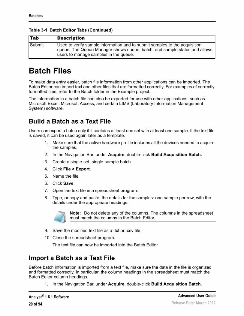
Batch FilesTo make data entry easier, batch file information from other applications can be imported. The Batch Editor can import text and other files that are formatted correctly. For examples of correctly formatted files, refer to the Batch folder in the Example project.
The information in a batch file can also be exported for use with other applications, such as Microsoft Excel, Microsoft Access, and certain LIMS (Laboratory Information Management System) software.
Build a Batch as a Text FileUsers can export a batch only if it contains at least one set with at least one sample. If the text file is saved, it can be used again later as a template.
1. Make sure that the active hardware profile includes all the devices needed to acquire the samples.
2. In the Navigation Bar, under Acquire, double-click Build Acquisition Batch.
3. Create a single-set, single-sample batch.
4. Click File > Export.
5. Name the file.
6. Click Save.
7. Open the text file in a spreadsheet program.
8. Type, or copy and paste, the details for the samples: one sample per row, with the details under the appropriate headings.
9. Save the modified text file as a .txt or .csv file.
10. Close the spreadsheet program.
The text file can now be imported into the Batch Editor.
Import a Batch as a Text FileBefore batch information is imported from a text file, make sure the data in the file is organized and formatted correctly. In particular, the column headings in the spreadsheet must match the Batch Editor column headings.
1. In the Navigation Bar, under Acquire, double-click Build Acquisition Batch.
Submit Used to verify sample information and to submit samples to the acquisition queue. The Queue Manager shows queue, batch, and sample status and allows users to manage samples in the queue.
Note: Do not delete any of the columns. The columns in the spreadsheet must match the columns in the Batch Editor.
Table 3-1 Batch Editor Tabs (Continued)
Tab Description
Analyst® 1.6.1 Software
20 of 94
Advanced User Guide
Release Date: March 2012

Batches
2. In the Sample tab, right-click and then click Import From > File.
3. Click the text file containing the batch information.
4. Click Open.
If an autosampler is being used, then the Select Autosampler dialog opens.
5. In the autosampler list, select the autosampler.
6. Click OK.
The sample table fills with the details from the text file.
Set Quantitation Details in the Batch Editor (Optional)If users do not want select quantitation details post-acquisition, then Quantitation methods can be included with a batch and used to define the quantitation details prior to submitting a batch.
Internal Standard and Standard columns appear in the Quantitation tab according to the quantitation method selected in the Sample tab.
1. With a batch file open in the Batch Editor window, click the Quantitation tab.
2. Select the set.
3. In the cell, select a Quant Type for all the samples.
4. If applicable, type the peak concentration in the Analyte column.
5. If applicable, type the Internal Standard.
6. Repeat the preceding steps for each set in the batch.
7. Save the file.
Note: If the saved text file is not visible, then in the Files of type list, select Microsoft Text Driver (*.txt; *.csv). Files with the extension .txt appear in the field.
Advanced User Guide
Release Date: March 2012Analyst® 1.6.1 Software
21 of 94

Batches
Analyst® 1.6.1 Software
22 of 94
Advanced User Guide
Release Date: March 2012

4
Device MethodsIf creating an acquisition method file from an existing file, the user can use some or all of the device methods in the acquisition method. Use the Acquisition Method Editor to customize the acquisition method by adding or removing device methods. If the required device icon is not in the Acquisition Method Browser pane, then users can add the device only if it is included in the active hardware profile.
Devices in Acquisition MethodsCreate an acquisition method for a device by selecting the operating parameters for that device. Acquisition methods can be created for any of the following devices if they are configured in the active hardware profile:
• Pumps.
• Autosamplers.
• Syringe pumps.
• Column ovens.
• Switching valves.
• Diode array detector.
• Analog-to-digital converters.
• Integrated systems.
For information about setting properties for devices, refer to the Peripheral Devices Setup Guide.
Add or Remove an LC Device 1. With a method file open in the Acquisition Method Editor, in the Acquisition method
pane, right-click Acquisition Method and then click Add/Remove Device Method.
Note: The available parameters for the LC devices vary depending on the manufacturer.
Advanced User Guide
Release Date: March 2012Analyst® 1.6.1 Software
23 of 94

Device Methods
Figure 4-1 Add/Remove Device Method dialog
2. Select or clear the check boxes beside the device method to add or remove the device method.
3. Click OK.
Set the LC Pump Properties1. With an acquisition method file open in the Acquisition Method Editor, in the
Acquisition method pane, click the Pump icon.
The Pump Properties tab opens in the Acquisition Method Editor pane.
2. Edit the fields as required.
3. Save the file.
Set the Autosampler Properties 1. Make sure that on the Acquisition Properties tab, the Synchronization Mode field
is set to LC Sync. The device and the instrument will start simultaneously.
2. With a method file open in the Acquisition Method Editor, in the Acquisition method pane, click the Autosampler icon.
The Autosampler Properties tab opens in the Acquisition Method Editor pane.
3. Edit the fields as required.
4. Save the file.
Set the Column Oven Properties1. With a method file open in the Acquisition Method Editor, in the Acquisition method
pane, click the Column Oven icon.
The Column Oven properties tab opens in the Acquisition Method Editor pane.
2. Edit the fields as required.
Analyst® 1.6.1 Software
24 of 94
Advanced User Guide
Release Date: March 2012

Device Methods
3. Save the file.
Set the Switching Valve Properties The switching valve can be used as a diverter or injection valve. Select the Manual Sync with Valve synchronization mode if using the valve as an injector; choose any other mode if using the valve as a diverter.
1. With a method file open in the Acquisition Method Editor, in the Acquisition method pane, click the Valve icon.
The Valve Properties tab opens in the Acquisition Method Editor pane.
2. Change the position names from their preset names, if required.
The switching valve is sometimes used to switch the flow of solvent to waste, or to a different column. The preset position names are A and B.
• In the Change Position Names list, select a position.
• In the Change Position Names list, rename the preset position names A and B to Inject and Divert or to Column and Waste, depending on how the valve is plumbed.
3. In the Total Time (min) column, click a cell, and then type the total time the valve will remain in this position.
4. In the Position column, click a cell and then, in the Position list, select the valve position.
5. Repeat the steps 3 and 4 for each switch of the valve required during acquisition.
6. Save the file.
Set the Diode Array Detector Parameters1. With a method file open in the Acquisition Method Editor, in the Acquisition method
pane, click the Diode Array Detector (DAD) icon.
The DAD Method Editor tab opens in the Acquisition Method Editor pane.
2. Set the desired acquisition parameters and save the file.
Set the Analog-to-Digital Converter Properties1. With a method file open in the Acquisition Method Editor, in the Acquisition method
pane, click the Analog to Digital Converter (ADC) icon.
The Analog/Digital Convertor Properties tab opens in the Acquisition Method Editor pane.
2. In the Sample section, in the Rate (pts/sec) field, type the rate.
3. Do the following to set the channel details:
Note: The interval and rate are proportional to each other. When the rate is changed, the software automatically calculates the interval again.
Advanced User Guide
Release Date: March 2012Analyst® 1.6.1 Software
25 of 94

Device Methods
• In the Channels field, click the channel name, and then select the check box beside the name to include it in the method.
• In the Interpreted Value @ Full Scale field, type the appropriate value.
• In the Interpreted Unit field, type the appropriate unit.
The number of available channels is specified when setting up the ADC in the hardware profile.
4. Save the file.
Analyst® 1.6.1 Software
26 of 94
Advanced User Guide
Release Date: March 2012

Device Methods
Dynamic Fill TimeDynamic Fill Time (DFT) is a feature specifically designed to optimize the data obtained in every spectrum for the linear ion trap scan functions. DFT will automatically adjust the fill time used to fill the ion trap based on the ion flux coming from the source. For more intense ions, the fill time will be automatically reduced to ensure the trap is not overfilled with ions.
For less intense ions, the fill time will be automatically increased, ensuring that good ion statistics are obtained in the spectrum. DFT is applicable for the following scan types:
• Enhanced MS (EMS)
• Enhanced Resolution (ER)
• Enhanced Product Ion Scan (EPI)
• MS/MS/MS (MS3)
Adjust the DFT settings by selecting Tools > Settings > Method Options in the software.
Experiments and PeriodsThe mass spectrometer acquisition method consists of experiments and periods. In the Acquisition Method Browser pane, create a sequence of acquisition periods and experiments for the instrument. Users can also open a method previously created in the Tune Method Editor.
ExperimentsAn experiment includes the instrument settings and the scan type during an MS scan. A set of MS scans performed for a specific amount of time is called a period. An acquisition method in which the MS parameters and actions are the same through the entire duration is called a single-period, single-experiment method.
In looped experiments, MS settings are changed on a scan-by-scan basis. For example, if the sample contains two compounds, A and B, users may want to loop an MS/MS experiment of compound A with an MS/MS experiment of compound B to obtain information about both compounds in the same run. The mass spectrometer method will alternate between the two scan types. Other examples of looped experiments include alternating between positive and negative modes in a run and Information Dependent Acquisition (IDA) methods.
PeriodsA period can contain one or more looped experiments. In a multi-period acquisition method, experiments are performed for a specified amount of time and then switch to another set of experiments. Periods are useful when the elution time of the compounds in an LC run is known. The instrument can perform different experiments according to when the compounds elute to obtain as much information as possible in the same run.
Figure 4-2 shows a three-period method. The first period has a duration of 3.015 minutes; the second period is 4.986 minutes; and the third period is 7.000 minutes.
Advanced User Guide
Release Date: March 2012Analyst® 1.6.1 Software
27 of 94

Device Methods
Figure 4-2 Example of a multi-period experiment
Information Dependent Acquisition MethodsInformation Dependent Acquisition (IDA) is an acquisition method that analyzes data during acquisition. IDA is used to change the experimental conditions depending on the analysis results. These real-time changes are controlled by criteria set in the acquisition method, including:
• Ion intensity and charge state.
• Inclusion and exclusion lists.
• Isotope pattern.
Optimizing data acquisition settings while the data is being acquired allows users to conserve both the sample and working time on an instrument.
Create an IDA method with up to two survey scans and eight dependent scans in a single experiment. A survey scan is used in IDA to trigger additional experiments. The following scan types can be used as a survey scan:
• Enhanced Multiply-Charged (EMC).
• Enhanced Product Ion (EPI) (second survey scan).
• Enhanced MS (EMS).
• MRM.
• Neutral Loss (NL).
• Precursor Ion (Prec).
• Q3 MS.
The following scan types can be used as dependent scans:
• EPI.
• MS/MS.
Analyst® 1.6.1 Software
28 of 94
Advanced User Guide
Release Date: March 2012
Device Methods
In an IDA experiment, the instrument actions are varied from scan type to scan type based on the data acquired in a previous scan. The software analyzes data as it is being acquired and then determines the masses on which to perform dependent scans. Uses can set the criteria that will activate an IDA experiment and the method parameters to be used.
IDA experiments modify experiments and improve results based on the following user-defined criteria:
• Ion intensity and charge state.
• Inclusion and exclusion lists.
• Isotope pattern.
• Dynamic exclusion.
• Rate of change in ion intensity (refer to Contour Plots on page 40).
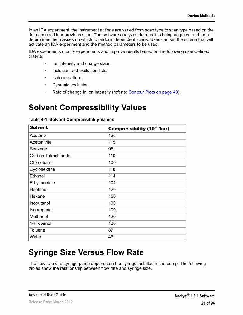
Solvent Compressibility Values
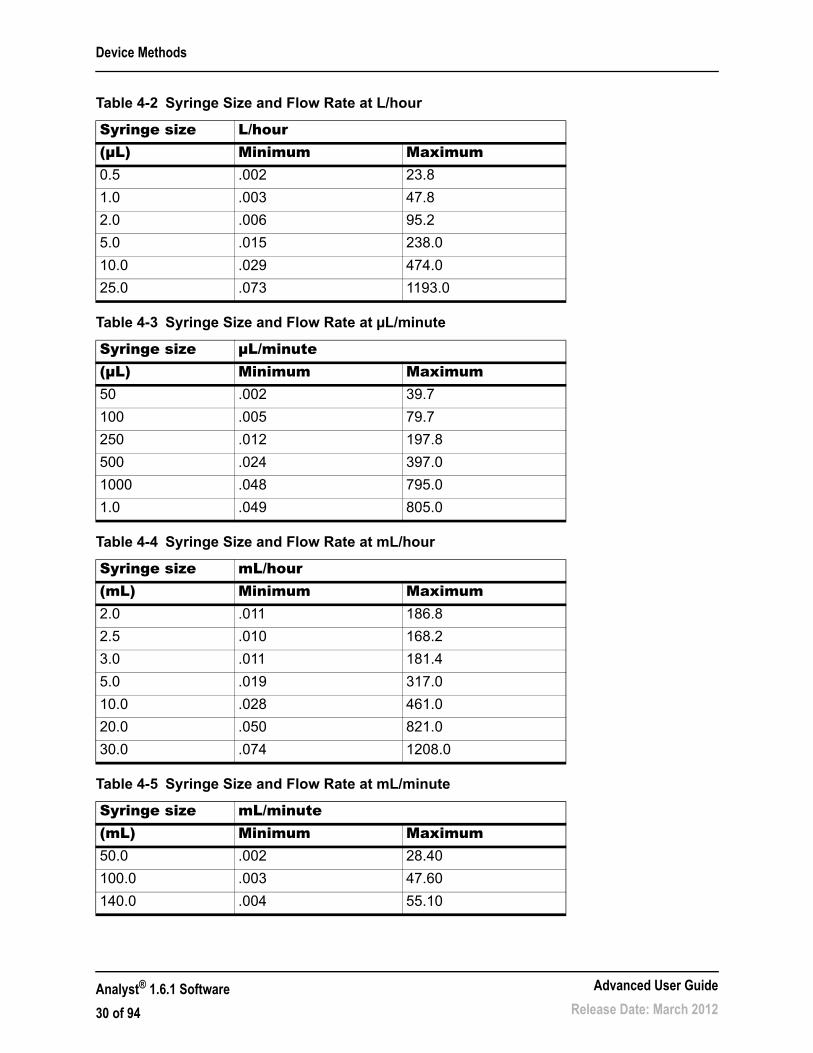
Syringe Size Versus Flow RateThe flow rate of a syringe pump depends on the syringe installed in the pump. The following tables show the relationship between flow rate and syringe size.
Table 4-1 Solvent Compressibility Values
Solvent Compressibility (10–6/bar)Acetone 126
Acetonitrile 115
Benzene 95
Carbon Tetrachloride 110
Chloroform 100
Cyclohexane 118
Ethanol 114
Ethyl acetate 104
Heptane 120
Hexane 150
Isobutanol 100
Isopropanol 100
Methanol 120
1-Propanol 100
Toluene 87
Water 46
Advanced User Guide
Release Date: March 2012Analyst® 1.6.1 Software
29 of 94
Device Methods
Table 4-2 Syringe Size and Flow Rate at L/hour
Syringe size L/hour(µL) Minimum Maximum0.5 .002 23.8
1.0 .003 47.8
2.0 .006 95.2
5.0 .015 238.0
10.0 .029 474.0
25.0 .073 1193.0
Table 4-3 Syringe Size and Flow Rate at µL/minute
Syringe size µL/minute(µL) Minimum Maximum50 .002 39.7
100 .005 79.7
250 .012 197.8
500 .024 397.0
1000 .048 795.0
1.0 .049 805.0
Table 4-4 Syringe Size and Flow Rate at mL/hour
Syringe size mL/hour(mL) Minimum Maximum2.0 .011 186.8
2.5 .010 168.2
3.0 .011 181.4
5.0 .019 317.0
10.0 .028 461.0
20.0 .050 821.0
30.0 .074 1208.0
Table 4-5 Syringe Size and Flow Rate at mL/minute
Syringe size mL/minute(mL) Minimum Maximum50.0 .002 28.40
100.0 .003 47.60
140.0 .004 55.10
Analyst® 1.6.1 Software
30 of 94
Advanced User Guide
Release Date: March 2012

5
Qualitative Data AnalysisUsers can view the information contained in a data file in table or graph form. Graphical data is presented either as a chromatogram or as a spectrum. Data from either of these displays can be viewed as a table of data points and various sorting operations can be performed on the data.
The software stores data in files with a .wiff extension. Wiff files can contain data for more than one sample. In addition to .wiff files, the software can open .txt files; .txt files contain data for only one sample. When a data file is opened in the software, different panes appear depending on the type of experiment that was performed.
If the MCA check box is selected in the Tune Method Editor, the data file will open to the MS (mass spectrum). If the MCA check box is not selected, then the data file opens with the Total Ion Chromatogram (TIC). Users can select a range and then double-click in the TIC pane at a particular time to show the MS for this range.
ChromatogramsA chromatogram displays the variation of some quantity with respect to time in a repetitive experiment; for example, when the instrument is programmed to repeat a given set of mass spectral scans several times. Chromatographic data is contiguous, even if the intensity of the data is zero. Chromatograms are not generated directly by the instrument, but are generated from mass spectra.
In the chromatogram display, the intensity, in counts per second (cps), is shown on the y-axis versus time on the x-axis. Peaks are automatically labeled.
In the case of LC/MS, the chromatogram is often displayed as a function of time, the time at which a particular scan was obtained, which can be derived from the scan number.
When data is viewed as a spectrum, mass-specific information about a compound is obtained. A chromatogram provides a general view of the data, usually time dependent when using an LC column, but it does provide information about the components of a peak. A spectrum, however, looks at a particular peak and provides the molecular weight of the corresponding compound, which can be used to find more specific information. For example, while a chromatogram may show only one peak, that peak can represent more than one compound; that is, different masses. A spectrum shows all of the masses that make up a peak, including the intensity of each mass.
Chromatographic data can change in both time and intensity if there is a change in the chromatographic conditions in a given sample. Spectral intensities may change, but the masses are fixed because the mass of a compound does not change.
There are two ways to generate spectral data:
• If only one scan is acquired, then the data is shown as a spectrum.
• From a chromatogram.
A typical spectrum is shown with the molecular weight, labeled with the m/z (mass-to-charge ratio), on the x-axis. The intensity is shown on the y-axis.
A chromatogram is a graphical display of the data obtained from the analysis of a sample. It plots the signal intensity along an axis that shows either time or scan number.
Advanced User Guide
Release Date: March 2012Analyst® 1.6.1 Software
31 of 94
Qualitative Data Analysis
The software plots intensity, in counts per second (cps), on the y-axis against time on the x-axis. Peaks above a set threshold are labeled automatically. In the case of LC/MS, the chromatogram often is shown as a function of time.
SpectraA spectrum is the data that is obtained directly from the instrument and normally represents the number of ions detected with particular mass-to-charge (m/z) values. It is displayed as a graph with the m/z values on the x-axis and intensity (cps) represented on the y-axis.
In the case of MS/MS data, the intensity is associated with two masses, the precursor ion mass (Q1) and the product ion mass or masses (Q3).
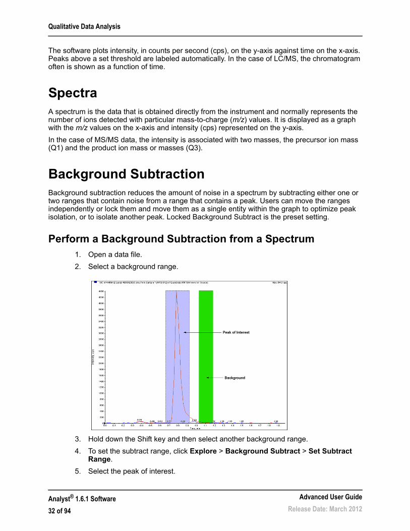
Background SubtractionBackground subtraction reduces the amount of noise in a spectrum by subtracting either one or two ranges that contain noise from a range that contains a peak. Users can move the ranges independently or lock them and move them as a single entity within the graph to optimize peak isolation, or to isolate another peak. Locked Background Subtract is the preset setting.
Perform a Background Subtraction from a Spectrum1. Open a data file.
2. Select a background range.
3. Hold down the Shift key and then select another background range.
4. To set the subtract range, click Explore > Background Subtract > Set Subtract Range.
5. Select the peak of interest.
Analyst® 1.6.1 Software
32 of 94
Advanced User Guide
Release Date: March 2012

Qualitative Data Analysis
6. Click Explore > Background Subtract > Perform Background Subtract.
The background is subtracted from the peak and a new spectrum is generated.
7. To isolate another peak, drag the locked ranges in the chromatogram and repeat the background subtract.
8. To save the background subtracted spectrum as a processed data file, click File > Save.
Unlock the RangesThe selected subtraction range is set to locked.
• Click Explore > Background Subtract > Subtract Range Locked.
The ranges are unlocked and each one can be moved independently.
Background Subtract to FileUse Background Subtract to File to save a new file that has a defined noise region subtracted from each scan. When a range is selected in the TIC, all the scans from that selection are internally averaged, and the resulting spectrum is subtracted from all the scans. Use the Background Subtract to File dialog to select where the file is to be saved. In some cases, the resulting file might look close to the original scan.
Perform a Background Subtraction to File1. Open a data file.
2. Select the background range within the TIC and set it as background.
3. Click Explore > Background Subtract to File.
Tip! To clear the background subtract region, click Explore > Background Subtract > Clear Subtract Range.
Advanced User Guide
Release Date: March 2012Analyst® 1.6.1 Software
33 of 94

Qualitative Data Analysis
Figure 5-1 Background Subtract to File dialog
4. In the Output Project and Filename section, type the project and file names for the resulting file.
5. Click Start Processing.
The progress bar displays the progress of the subtraction process. If the Open the new file immediately in Analyst check box is selected, then when the subtraction is complete, the file will appear.
6. If the check box is cleared, when the subtraction is complete, click Finish.
Baseline SubtractBaseline subtract removes a constant or slowly varying offset from a set of data. This is useful in locating small peaks that are obscured by noise. The software uses the following algorithm in performing a baseline subtraction.
• Every data point in the data set is considered as the center of a window (in mass or time) with a user-definable width measured in amu or minutes.
• The minimum values on either side of the current data point (minima) within the window are located.
• A straight line is fitted between the two minima and the height (intensity) of the current data point above the line is calculated. The end points of the data are regarded as minima.
• The data point is replaced with the new calculated value.
Analyst® 1.6.1 Software
34 of 94
Advanced User Guide
Release Date: March 2012

Qualitative Data Analysis
CalculatorsUsers can perform calculations on the basis of collected data. Although the calculator is a separate window, it is connected to the active graph within the software.
The following calculators are available.
• Elemental Composition Calculator
• Hypermass Calculator
• Elemental Targeting Calculator
• Mass Property Calculator
• Isotopic Distribution Calculator
Users can cut and paste from one text box to another between the different windows in the calculators. Data from any of the calculators can be printed by clicking the Print icon in the top left corner of the window. For more information about using calculators, refer to the Help.
Data from the Elemental Composition, Mass Property, and Isotopic Distribution calculators can be exported to a separate file. Use the Elemental Targeting calculator to modify the data within the active graph. Data from the HyperMass and Isotopic Distribution calculators can be overlaid on the active spectrum.
Elemental Composition CalculatorThe Elemental Composition calculator determines potential molecular or amino acid compositions based on a target mass-to-charge ratio. Type this ratio manually or select it from an active spectrum. This calculator creates a table with the possible element or amino acid combinations making up the mass of interest and the characteristics of each.
Type or select values for such parameters as tolerance, electron state, and number of charges. Users can also type a list of possible elements and put a limit on the number of each.
Hypermass CalculatorThe Hypermass calculator determines the distribution of a multiply charged envelope based on an uncharged mass. Users can select the uncharged mass, including the adduct and its polarity. The calculator displays a graphical representation of the Hypermass series, which can be overlaid onto the active spectrum. A list of the Hypermass data is also available.
Elemental Targeting CalculatorThe Elemental Targeting calculator reduces the data spectrum based on a specific pattern, primarily one corresponding to isotopic distributions. It can also search an MS data spectrum for a specific pattern of peaks, which can be entered either as a formula or as an isotopic distribution.
If the calculator finds a match, it creates a reduced plot containing only data pertaining to the specified pattern. For a spectrum, the calculator removes all unmatched data. For a
Tip! Set the precision of calculator data in the Calculators tab of the Appearance Options dialog. To open the dialog, click Tools > Settings > Appearance Options.
Advanced User Guide
Release Date: March 2012Analyst® 1.6.1 Software
35 of 94
Qualitative Data Analysis
chromatogram, the calculator calculates the elemental target for each of the underlying spectra and regenerates each point in the chromatogram on the basis of these new spectra.
Mass Property CalculatorThe Mass Property calculator determines various properties such as exact mass, the average mass, the mass accuracy, and the mass defect of a mass of interest. The results generated by this calculator depend upon the number of input fields completed.
Isotopic Distribution CalculatorThe Isotopic Distribution calculator determines the isotopic distribution based on an entered formula. This allows users to distinguish between compounds with the same mass based on relative intensities of isotopes.
The calculated isotopic distribution can be displayed in graphical or text format on the Isotopic Distribution pane, overlaid on the active spectrum, or exported to a separate file.
Centroided PeaksCalculating the centroid of a peak converts peak distribution values into a single value of m/z and intensity that represents the peak. Centroided data collected in profile mode simplifies the data and reduces the file size. Centroided data provides more accurate peak assignment and reduces the amount of data, but it also removes the information about the peak shape.
The centroid algorithm converts peaks to single values by using an intensity weighted average to calculate the center of gravity of the peak. The output of the algorithm is a list of peaks with parameters, as shown in Table 5-1.
Data is automatically calculated as a centroid when added to a library or when a search is conducted.
Calculate the Centroid of a Peak1. Select a pane containing a spectrum.
Calculating the centroid of the peak changes the appearance of the existing graph. To compare the result with the original data, make a copy of the graph before calculating the centroid.
2. Click Explore > Centroid.
Table 5-1 Peak Parameters
Parameter DefinitionCentroid Value The value of the centroided data in units of mass or time.
Intensity The intensity of each peak in cps.
Width The width of the centroided peak in amu.
Analyst® 1.6.1 Software
36 of 94
Advanced User Guide
Release Date: March 2012

Qualitative Data Analysis
Figure 5-2 Analyte Centroid Location
Data AnalysisUsers can open files containing existing data or data that is currently being acquired. All experiment-related data can also be viewed in tabular form. The table pane consists of two tabs, the Data List tab and the Peak List tab.The Data List tab contains experiment-related information, such as acquisition time and scan intensity. The Peak List tab displays peak-related information such as peak height, peak area, and baseline type.
Total Ion ChromatogramA Total Ion Chromatogram (TIC) is created by summing the intensity contributions of all ions from a series of mass scans. Users can use the TIC to view an entire data set in a single pane. It consists of the summed intensities of all ions in a scan plotted against time in a chromatographic pane. If the data contains results from multiple experiments, individual TICs (Total Ion Chromatograms) for each experiment and another TIC that represents the sum of all experiments can be created. The preset TIC that represents the sum of all of the experiments is shown with a splitter tool below the center of the x-axis.
Extracted Ion ChromatogramAn Extracted Ion Chromatogram (XIC) is an extracted ion chromatogram created by taking intensity values at a single, discrete mass value, or a mass range from a series of mass spectral scans. It shows the behavior of a given mass, or mass range, as a function of time. The intensity of the ion, or the summed intensities of all ions in a given range, is plotted in a chromatographic pane.
Base Peak ChromatogramA Base Peak Chromatogram (BPC) displays the intensity of the most intense ion in every scan as a function of scan number or retention time. It is useful in instances where the TIC is so dominated by noise that there is a large offset and chromatographic peaks are hard to distinguish. It is also helps to distinguish between co-eluting components. BPCs only be generated from single period, single experiment data.
A1
A1=A2
Time
A2
Centroid Location
Advanced User Guide
Release Date: March 2012Analyst® 1.6.1 Software
37 of 94
Qualitative Data Analysis
The graph uses two colors, alternating each time the mass of the base peak changes. The color changes are maintained when the data is manipulated by scrolling or zooming. For information about selecting the colors used in the graph, refer to the Help.
Extracted Wavelength ChromatogramAn Extracted Wavelength Chromatogram (XWC) is a wavelength chromatogram created by taking intensity values at a single wavelength, or by the sum of the absorbance for a range of several wavelengths
Diode Array DetectorUsers can view the Diode Array Detector (DAD) spectrum for a single point in time, or for a range of time as a Total Wavelength Chromatogram.
Total Wavelength ChromatogramA Total Wavelength Chromatogram (TWC) is a less commonly used chromatogram. It displays the total absorbance (mAU) as a function of time. The TWC provides a way of viewing an entire data set in a single pane. It consists of the summed absorbances of all ions in a scan plotted against time in a chromatographic pane. If the data contains results from multiple experiments, individual TWCs for each experiment and another TWC that represents the sum of all experiments can be created.
Overlay GraphsTwo or more sets of data can be visually compared by overlaying graphs created by similar methods. Each individual spectrum is distinguished by the color of its trace. For full scan data, this allows users to visualize the differences between several sample spectra.
If one or more panes are chosen, then each XIC will appear in a separate pane.
1. Select the first pane to be overlaid.
2. Click Explore > Overlay.
3. Click in the second pane.
The graphs are overlaid showing the two traces in different colors.
Tip! To overlay fewer than four graphs in the same pane, press Ctrl + right-click in a pane and then click Appearance Options. In the Appearance Options dialog, Multiple Graph Options tab, select Yes for the Overlay Multiple Panes fields for Spectrum and Chromatogram.
Tip! To view a color-coded list of the overlaid graphs, right-click the title bar of the pane.
Analyst® 1.6.1 Software
38 of 94
Advanced User Guide
Release Date: March 2012

Qualitative Data Analysis
Cycle Between Overlaid Graphs1. Select a pane that contains overlaid graphs.
2. Click Explore > Cycle Overlays.
The display changes so that the next graph in sequence is shown in the foreground.
Sum OverlaysIf two or more graphs overlaid are overlaid, users can sum the graphs to get a new trace. Each point on the new trace is the sum of the points from the graphs. Summing several overlays of similar data type can make subsequent processing operations easier and faster. For example, users can overlay several XICs, sum them, and then smooth the summed overlay to remove noise.
Summing overlays is similar to generating a TIC with the benefit of being able to choose which graphs to overlay. For example, if ten experiments are being viewed, the TIC will add all ten experiments together. If overlays are summed, then users have the option of adding only nine of the ten overlaid graphs. This procedure can be used if the data collected in the one experiment is just noise.
1. Overlay the graphs that are to be summed.
2. Click Explore > Sum Overlays.
The overlaid graphs are added together.
Graphs LabelsGraphs can be customized using the preset style for labels on graphs and chromatograms. Users can select the fonts to use for peak and axis labels, and the colors to use for the traces. Users can also add axis labels and the type of label and precision for the peaks.
Add Captions to a GraphUse captions to label peaks of interest or significant points on the graph. When a caption is placed beside a peak, the caption stays with the peak when the graph is zoomed in or out. Captions also stay with the original sample when users navigate between samples in a data file. A caption contains one line of text, with a maximum of 128 characters.
1. In the spectrum, right-click, and then click Add Caption.
The Add Caption dialog opens.
2. In the Caption box, type the text.
3. To change the size and style of the caption, click Font.
4. To place the caption, click OK.
Tip! If the position of the caption is not satisfactory, then drag the caption to a different position. The caption stays in the same place relative to the x- and y-axes when the graph is zoomed in or out. To edit or delete the caption, right-click the caption and then click the appropriate command.
Advanced User Guide
Release Date: March 2012Analyst® 1.6.1 Software
39 of 94

Qualitative Data Analysis
Add Text to a GraphUse text to add multiple lines of information to a graph. Unlike captions, which are associated with a specific peak and move with it as the graph is zoomed, text labels remain in their original location as the graph is zoomed. They do not stay with the original sample when users navigate between samples in a data file.
1. In the graph, right-click and then click Add User Text.
The Add User Text dialog opens.
2. In the User Text field, type the text.
3. To center the text, select the Center Text check box.
4. To change the size and style of the caption, click Font.
5. To insert the text, click OK.
Compound DatabaseThe compound database stores information about compounds, including optimization specifications. Use the compound database when there is a large numbers of samples and a large number of compounds need to be optimized quickly. The Compound Database window stores optimized conditions for compounds that can be retrieved to run samples.
Contour PlotsA Contour Plot is a color-coded plot of a complete data set that uses color to represent a third dimension in the plot. In a Contour Plot of a TIC, the x-axis represents retention time or scan number, the y-axis represents mass, and the color represents the intensity of the data at that point. In a Contour Plot of a TWC for DAD data, the x-axis represents retention time or scan number, the y-axis represents wavelength, and the color represents absorbance. The Contour Plot is a post-acquisition tool that does not function in a real-time scan acquisition.
Color is the third axis in Contour Plot, and it represents either intensity or absorbance. Users can change the high and low intensity or absorbance values in Contour Plot using the control triangles on the color bar above the Contour Plot. The percentage parameters at the top of the Contour Plot pane indicate the values held by the low and high sliders. The actual values are based on a percentage of the maximum intensity or absorbance within the selected area. The value is shown in the top right corner of the Contour Plot pane.
The controls shown in Figure 5-3 change the colors in a Contour Plot.
Tip! If the position of the text is not satisfactory, then drag the text to a different position. To edit or delete the text, right-click the text and then choose the appropriate command.
Note: The Contour Plot does not support MI or MRM scans, but it does support DAD scans.
Analyst® 1.6.1 Software
40 of 94
Advanced User Guide
Release Date: March 2012

Qualitative Data Analysis
Figure 5-3 Buttons Controlling Contour Plot Colors
Users can define the colors on a Contour Plot graph to provide better contrast and display data specifications according to their needs. For example, setting the intensity/wavelength and changing the color of the values for Below Low Data and Above High Data can eliminate background noise in a Contour Plot.
The Below Low Data and Above High Data buttons shrink and expand on the color bar if the slider controls are moved. When the contour plot colors are changed, the new colors become the preset colors for all subsequent graphs.
View a Contour PlotA Contour Plot can be viewed only after acquisition. Users can view a Contour Plot from TIC, XIC, TWC, or XWC graphs. TICs and XICs are available for all .wiff data files. TWCs and XWCs are available only for data acquired by a DAD.
1. In Explore mode, open a data file as a TIC, XIC, TWC, or XWC graph.
2. Highlight the range to be viewed in the Contour Plot. If a selection is not made, the entire range is viewed.
3. Click Explore > Show > Show Contour Plot.
A Contour Plot of the selected area opens in a separate pane.
Select an Area in a Contour PlotTo zoom in on a particular selection, or view the corresponding mass spectrum for that selection, do one of the following:
Table 5-2 Right-Click Menu for Contour Plot Panes
Menu FunctionShow DAD Spectrum Opens a new pane with the DAD spectrum.
Extract Wavelengths (Use Range)
Extracts up to three wavelength ranges from a DAD spectrum to display the XWC.
Extract Wavelengths (Use Maximum)
Extracts wavelength ranges using the maximum wavelengths.
Zoom to selection Zooms in on the selected area.
Add User Text Adds a text box at the position of the cursor.
Undo Zoom Returns the graph to the original scale
Delete Pane Deletes the selected pane
Show Cross-Hair Shows the Cross-Hair (nm/min)
Advanced User Guide
Release Date: March 2012Analyst® 1.6.1 Software
41 of 94
Qualitative Data Analysis
• To select a standard area within a box, drag the pointer to create a box around an area in the Contour Plot.
• To make a vertical selection, press Ctrl and drag the pointer vertically.
• To make a horizontal selection, press the space bar and drag the pointer horizontally.
Set the Intensity and Absorbance in a Contour Plot• Do one of the following:
• To set the low intensity/absorbance value in a Contour Plot, from the color bar above the Contour Plot, drag the left triangular slider to the required position.
Contour Plot automatically adjusts the color of values below the setting to indicate they are outside the range.
• To set the high intensity/absorbance value in a Contour Plot, from the color bar above the Contour Plot, drag the right triangular slider to the required position.
The Contour Plot automatically adjusts the color of values above the setting to indicate they are outside the range.
Change Colors in a Contour Plot
1. In the Contour Plot pane, click one of the color buttons.
The Color dialog opens.
2. Click a color.
3. Click OK.
The graph changes to reflect the color change.
Dynamic Background Subtraction AlgorithmDynamic Background Subtraction™ algorithm improves detection of precursor ions in an IDA (Information Dependant Acquisition) experiment. When the algorithm is activated, IDA uses a spectrum that has been background subtracted to select the ion of interest for MS/MS analysis, as opposed to selecting the precursor from the survey spectrum directly. Because this process takes place during LC analysis, the algorithm enables detection of species as their signal increases in intensity, therefore focusing on detection and analysis of the precursor ions on the rising portion of the LC peak, up to the top of the LC peaks (maximum intensity).
Fragment InterpretationThe Fragment Interpretation tool helps the user interpret MS/MS data. Given the chemical structure of a molecule, this tool can generate a list of theoretical fragment masses from single
Tip! By using the Define Custom Colors palette, users can create customized colors for use in a Contour Plot.
Analyst® 1.6.1 Software
42 of 94
Advanced User Guide
Release Date: March 2012
Qualitative Data Analysis
non-cyclic bond cleavage of that molecular structure. The tool can then match the theoretical list with peaks in the current mass spectrum.
The Fragment Interpretation Tool generates a list of theoretical fragment masses from single, non-cyclic bond cleavage of a molecular structure. The molecular structure can be created in a third-party drawing program and then saved as a .mol file. Fragment Interpretation displays the theoretical fragments in the fragment list and compares the fragment masses to peaks in the mass spectrum. Peaks above the threshold intensity and within the user-defined mass tolerance (maximum 2 amu) of fragment masses are considered matched and appear in bold text in the fragment list.
• Precursor Ion
• Neutral Loss
• Q1 Multiple Ion
• Q3 Multiple Ion
• Multiple Reaction Monitoring (MRM)
Connect the Fragment Interpretation Tool to a SpectrumWhen a single, non-cyclic bond in the molecular structure is selected, the Fragment Interpretation tool highlights the two fragments created when the bond is cleaved and matching peaks in the connected spectrum are displayed.
If multiple spectrum panes are being viewed, then the Fragment Interpretation tool connects to the active spectrum. If the data file contains more than one sample, then the Fragment Interpretation tool connects to the active spectrum.
If a spectrum is open when the Fragment Interpretation tool is opened, then the active panel links to the open spectrum automatically.
1. Click Explore > Show > Show Fragment Interpretation Tool.
2. From the lower right corner of the Fragment Interpretation pane, click the connect button.
The pointer changes to the connecting tool.
3. Click the spectrum graph that is to be connected to the Fragment Interpretation tool.
The connected graph indicator in the lower left corner contains the name of the graph connected to the Fragment Interpretation pane. The connection is broken when either the graph or Fragment Interpretation is closed. If the connected .wiff file has more than one sample, the Fragment Interpretation pane updates automatically as users scroll through the samples.
Note: The Fragment Interpretation tool cannot be used with the following scan types:
Advanced User Guide
Release Date: March 2012Analyst® 1.6.1 Software
43 of 94

Qualitative Data Analysis
Match Fragments with Peaks1. Click Explore > Show > Show Fragment Interpretation Tool.
2. With a .mol file in the Fragment Interpretation pane, select a cell in the Fragment List that is shown in bold.
In the spectrum, the software highlights the matching spectral peak in the color selected under the Options tab. In the molecular structure, the bond is highlighted.
3. If a row that has more than one matching fragment is clicked, the spectral peak that is closest to its monoisotopic mass is highlighted in the mass spectrum in the color specified in the Options tab.
Select a Bond in a Molecular Structure1. Click Explore > Show > Show Fragment Interpretation Tool.
2. With a .mol file opened in the Fragment Interpretation pane, click a single, non-cyclic bond in the molecular structure.
The two resulting fragments appear as highlights in the fragment list. The masses of the two fragments appear on either side of the bond.
If a spectrum is connected, then the Fragment Interpretation tool displays any matching peaks in the graph. If a fragment in the list is selected and the fragment is matched to a peak, then the Fragment Interpretation window zooms in on that peak.
View IsotopesThe Fragment Interpretation tool can display the theoretical isotopic distribution for a peak matching a fragment in the fragment list.
1. Click Explore > Show > Show Fragment Interpretation Tool.
2. In the Fragment Interpretation pane, click the Options tab.
3. Select the Show Isotopes check box.
4. Click Apply.
5. In the fragment list, select a fragment that matches a peak.
The isotopic distribution for matched peaks is shown in the spectrum.
Display a Formula Difference in a SpectrumThe formula and monoisotopic mass difference between two related hypothetical fragments can be displayed. The formula difference is shown when two peaks are selected. The formula and monoisotopic mass difference is shown when two fragments are selected, or two single, non-cyclic bonds.
1. Click a fragment peak.
2. Press the Shift key and then click another fragment peak.
If the formula difference is equal to a fragment from the fragment list, the fragment highlights in the list. Otherwise, the formula difference between the matching fragments of the peaks is shown in a message box.
Analyst® 1.6.1 Software
44 of 94
Advanced User Guide
Release Date: March 2012
Qualitative Data Analysis
Display a Formula Difference in the Fragment List1. Click the row number for one fragment.
2. Press the Ctrl key and then click another fragment.
The formula and monoisotopic mass difference is shown in a message box if the fragments are related.
Display a Formula Difference in a Molecular Structure1. Click a single, non-cyclic bond. The preset fragment (of the two highlighted
fragments) is selected. To select the other fragment of the cleaved bond, CTRL+click the bond.
2. Select a second non-cyclic bond. To select the preset fragment, press the Shift key and then click the bond. To select the other fragment of the cleaved bond, press Ctrl+Shift+click the bond.
Fragment Interpretation calculates the formula and monoisotopic mass difference between the fragment selected in step 1 and the fragment selected in step 2, if the fragments are related. The formula and monoisotopic mass difference is shown in a message box.
IDA ExplorerThe Information Dependent Acquisition (IDA) Explorer is used to display data acquired through an IDA method.
The IDA Explorer can be turned off and on in the IDA Explorer tab in the Appearance Options dialog. Columns present in the List View can be defined in this tab as well.
The left side of the viewer shown in Figure 5-4 displays the masses on which a product ion scan was performed. In this area, users can examine the mass, intensity, time, and collision energy of ions on which product ion scans were performed in either a list view or a tree view. In list view, the list can be sorted by double-clicking on any column header. Use the Appearance Options dialog to customize the columns in the list view.
On the right side, the viewer is split into four panes. The top left pane displays the survey TIC data. The bottom left pane shows the XIC of the mass. The top and bottom right panes show the survey and product scans, respectively.
The IDA viewer lists all the masses on which Enhanced Product Ion scans or Enhanced Resolution scan types were performed. In the IDA viewer, users can do the following:
• Click a mass in the list or tree view to display plots relevant to that mass.
• View the survey spectrum from which the mass was identified and the product spectrum of that mass.
• Display the TIC of the survey scan and the XIC for each mass.
Note: Brackets around a mass indicate that the mass is merged. A merged mass is contiguous across a number of cycles. When a merged mass is displayed, it indicates an averaged spectrum, containing the average of all contiguous spectra.
Advanced User Guide
Release Date: March 2012Analyst® 1.6.1 Software
45 of 94

Qualitative Data Analysis
Figure 5-4 IDA Viewer
Library DatabasesThe Library Search feature compares unknown spectra to known MS spectra contained in a library database and generates a list of possible matches. Use Library Search to create and manage a mass spectra database that can be used to search for and match unknown spectra against the mass spectra stored in the database.
With Library Search users can:
• Compare library contents against an unknown spectrum.
• Add records to the library.
• Edit existing records.
Library data can be stored in the following locations:
• MS Access on a local database.
• MS SQL Server.
Before using the Library Search feature, determine where the library database is stored and connect the computer to that location. Library databases can be stored locally and over a network.
Use an alias to connect to a database. In this case, the alias specifies a connection to a specific database and may include the user name and password required to access the database. For example, a user may have a small library database of identified compounds on a computer and the company may have a central database that is used occasionally by the users. Creating
Analyst® 1.6.1 Software
46 of 94
Advanced User Guide
Release Date: March 2012
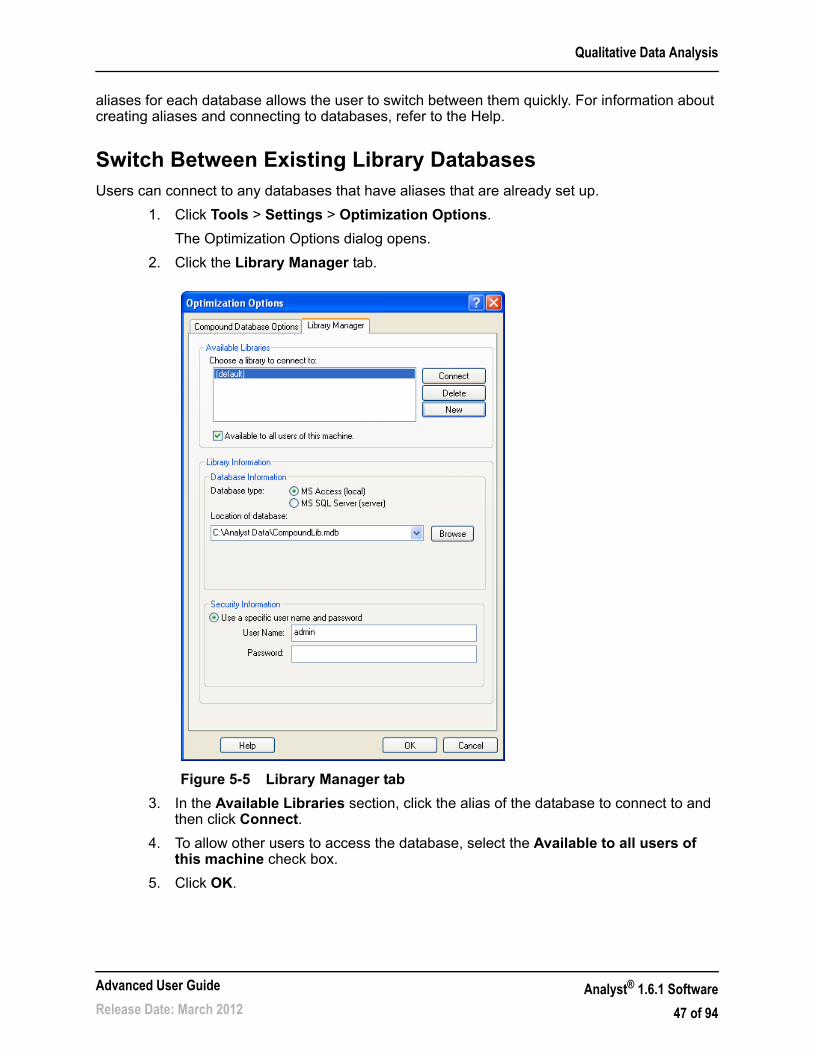
Qualitative Data Analysis
aliases for each database allows the user to switch between them quickly. For information about creating aliases and connecting to databases, refer to the Help.
Switch Between Existing Library DatabasesUsers can connect to any databases that have aliases that are already set up.
1. Click Tools > Settings > Optimization Options.
The Optimization Options dialog opens.
2. Click the Library Manager tab.
Figure 5-5 Library Manager tab
3. In the Available Libraries section, click the alias of the database to connect to and then click Connect.
4. To allow other users to access the database, select the Available to all users of this machine check box.
5. Click OK.
Advanced User Guide
Release Date: March 2012Analyst® 1.6.1 Software
47 of 94

Qualitative Data Analysis
Connect to a Local Library Database1. Click Tools > Settings > Optimization Options.
The Optimization Options dialog opens.
2. Click the Library Manager tab.
3. In the Available Libraries section, click New.
Figure 5-6 Add Library dialog
4. Type a name for the library.
5. In the Database Information section, select MS Access (local).
6. Type the database location.
7. In the Security Information section, if required, type a user name and password to access the database.
8. Click Save.
Connect to a Server Library Database1. Click Tools > Settings > Optimization Options.
The Optimization Options dialog opens.
2. Click the Library Manager tab.
3. In the Available Libraries section, click New.
Analyst® 1.6.1 Software
48 of 94
Advanced User Guide
Release Date: March 2012
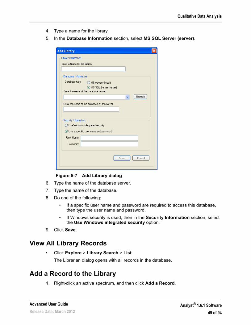
Qualitative Data Analysis
4. Type a name for the library.
5. In the Database Information section, select MS SQL Server (server).
Figure 5-7 Add Library dialog
6. Type the name of the database server.
7. Type the name of the database.
8. Do one of the following:
• If a specific user name and password are required to access this database, then type the user name and password.
• If Windows security is used, then in the Security Information section, select the Use Windows integrated security option.
9. Click Save.
View All Library Records• Click Explore > Library Search > List.
The Librarian dialog opens with all records in the database.
Add a Record to the Library1. Right-click an active spectrum, and then click Add a Record.
Advanced User Guide
Release Date: March 2012Analyst® 1.6.1 Software
49 of 94
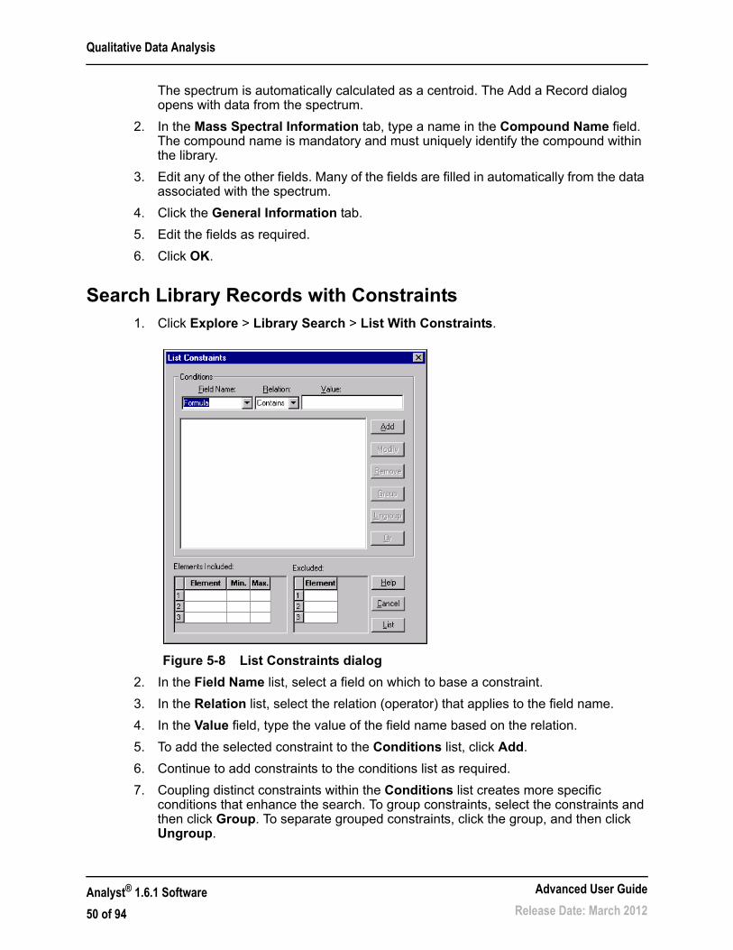
Qualitative Data Analysis
The spectrum is automatically calculated as a centroid. The Add a Record dialog opens with data from the spectrum.
2. In the Mass Spectral Information tab, type a name in the Compound Name field. The compound name is mandatory and must uniquely identify the compound within the library.
3. Edit any of the other fields. Many of the fields are filled in automatically from the data associated with the spectrum.
4. Click the General Information tab.
5. Edit the fields as required.
6. Click OK.
Search Library Records with Constraints1. Click Explore > Library Search > List With Constraints.
Figure 5-8 List Constraints dialog
2. In the Field Name list, select a field on which to base a constraint.
3. In the Relation list, select the relation (operator) that applies to the field name.
4. In the Value field, type the value of the field name based on the relation.
5. To add the selected constraint to the Conditions list, click Add.
6. Continue to add constraints to the conditions list as required.
7. Coupling distinct constraints within the Conditions list creates more specific conditions that enhance the search. To group constraints, select the constraints and then click Group. To separate grouped constraints, click the group, and then click Ungroup.
Analyst® 1.6.1 Software
50 of 94
Advanced User Guide
Release Date: March 2012

Qualitative Data Analysis
8. To change the relationship between constraints, click the relationship, and then click And or Or.
9. To exclude compounds containing a certain number of atoms of specific elements, select or type the elements in the Elements Included table, and then type a minimum and maximum number of atoms of the element.
10. To exclude compounds containing certain elements, select or type the elements in the Excluded table.
11. To search for compounds fitting the criteria, click List.
Records that match all the constraints appear in the Records table. Listing constraints are saved.
Library Search Tips
Search for a Similar SpectrumThe user can search the library for a spectrum and its related compound information that matches, or is similar to, an active spectrum. Searches can be performed with or without constraints. When the user searches with constraints, only those records that match all the criteria appear. The results appear in a ranked list; the first item on the list is the best fit to the active spectrum. Entries lower in the list do not match as well.
The more constraints that are selected, the more precise the list becomes and fewer, more relevant matches appear. After a set of constraints is defined, they will apply to all subsequent searches, unless they are edited. When a user searches without constraints, there is a much larger list of suggested spectra because the library makes fewer specific matches to the spectral data.
Only peaks above the threshold are used in the search. When selecting search constraints, The user can also add or subtract peaks from the active spectrum.
For example, if the user thinks a peak is actually a background or noise spike, the peak should not be used for the search because it could produce inaccurate results.
1. Right-click on an active spectrum and then click Search With Constraints.
The software calculates the centroid of the spectrum automatically.
Note: Element symbols are case-sensitive. For example, Hydrogen is H, not h and Sodium is Na, not NA or na.
Table 5-3 Library Search Tips
To do this... ... do thisGroup conditions. Select the conditions to group and then click Group. This
function behaves like parentheses in formulas.
Search without using constraints.
Right-click an active spectrum, and then click Search Library. The Search Results dialog opens.
Advanced User Guide
Release Date: March 2012Analyst® 1.6.1 Software
51 of 94

Qualitative Data Analysis
Figure 5-9 Search Constraints dialog
2. In the Maximum Number of Match field, type the maximum number of compounds to be returned by the search.
3. In the Preselect Constraints section, select the check boxes for the constraints to apply.
4. For each constraint selected, in the Preset Tolerance section, type the tolerance.
5. If required, select a method of sorting records from the Result Sorted by list.
6. If required, type text in the Comment Contains field.
7. If required, type text in the Keyword Contains field.
8. To apply peak constraints by adding and removing peaks, click Peak Constraints.
The Peaks Included table opens.
9. To add peaks to the list to search against, click Add and then type the m/z and the corresponding intensity in the empty cell.
10. To remove peaks so that they will not be included in the search, select the peaks and then click Remove.
11. Click Search to save the constraints and begin the search.
Analyst® 1.6.1 Software
52 of 94
Advanced User Guide
Release Date: March 2012
Qualitative Data Analysis
View a Compound from the Search ResultsIf several spectra match the unknown spectrum, the user may want to view other spectra and compare them to the unknown.
1. In the Search Results dialog, in the list of compounds, select the row number of the compound.
2. Click the spectrum pane of one of the known compounds.
The spectrum of the selected compound is shown.
Processed Data FilesThe user can save processed data, such as specific layouts and captions, that can be opened in Explore mode only. These files also contain history information and are similar to data files except that they will contain only the data from the active pane in Explore. These files have the .pdt extension and are stored in the Data folder in the current project.
Save a Processed Data File1. Select the pane.
2. Click File > Save Processed Data File.
3. In the File name field, type a name.
4. Click Save.
Open a Processed Data File1. In Explore mode, click File > Open Processed Data File.
2. Select a file.
3. Click Open.
Qualitative DataThe user can view the information contained in a data file in table or graph form. Graphical data is shown as a chromatogram or as a spectrum. Data in a table is shown as data points. The user can perform various sorting operations on the data.
When the user opens a data file, different panes appear depending on the type of experiment performed.
If the MCA check box is selected in the Tune Method Editor, the data file opens with the mass spectrum. If the MCA check box is not selected, the data file opens the TIC.
A wiff file can contain data for more than one sample. In addition to .wiff files, the software can open .txt files. A .txt file contains data for only one sample.
Advanced User Guide
Release Date: March 2012Analyst® 1.6.1 Software
53 of 94
Qualitative Data Analysis
Signal-to-Noise RatioThe signal-to-noise ratio is the peak height divided by the noise.
To calculate the noise, the software uses the standard deviation (using a mean of zero) of all data points in the chromatogram from the Background Start to Background End time (both shown in the advanced parameters for the Quantitation Method Editor and Peak Review window.) These times are set when a new background range is defined.
If the user builds a method without defining a new background range, which is possible if the preset integration is accepted with no changes, then the value for both the Background Start and the Background End is shown as N/A. As a result, the signal-to-noise ratio is not calculated and the corresponding field in the Results Table is shown as N/A.
Smoothing AlgorithmsThe user can select either the smoothing algorithm or the Gaussian smoothing algorithm as the smoothing method. The smoothing operation involves replacing each data point with the average of the data point before and after it. The smoothed data set replaces the old set.
Data can be smoothed more than once, but the software can undo only the last smooth. Smoothing is not available for multiple ion or MRM spectra.
Smooth Algorithm
When smoothing data, the user sets the point weighting values for three data points; the current point, the preceding point, and the following data point. The smooth algorithm multiplies the data points by the assigned weighting values, sums these values, and then divides the total by the sum of the point weight values. It is a gentler smooth than the Gaussian algorithm and it takes a long time to smooth very noisy data.
Gaussian Smoothing Algorithm
Gaussian smoothing involves replacing each data point with the weighted average of a number of data points on either side of it. The weighting for each new data point is calculated on the basis of a Gaussian curve. It is a coarser smooth than the smooth algorithm, but it is good for smoothing very noisy data.
Set two values when using the Gaussian smoothing method:
Gaussian filter width (% of minimal distance between points): This value shows the width used to calculate the weighting of neighboring points. The width is described in terms of percentages of the distance between two points in the scan, where the preset width of 100% gives a distribution that is as wide as the distance between data points.
Limit of Gaussian filter (number of minimal distance between points): This value corresponds to the limits of the Gaussian curve, shown in multiples of the distance between points. For example, the preset value of 10 creates a Gaussian curve that truncates after ten data point widths on either side of the center.
Analyst® 1.6.1 Software
54 of 94
Advanced User Guide
Release Date: March 2012

Qualitative Data Analysis
Smooth Data using the Smooth Algorithm
1. Select a pane containing a chromatogram or spectrum.
2. Click Explore > Smooth.
Figure 5-10 Smoothing Options dialog
3. Type the weighting factor in the following fields.
• Previous Point Weight field
• Current Point Weight field
• Next Point Weight field
4. Click OK.
The data set is smoothed, replacing the current data set in the pane.
Smooth Data using Gaussian Smoothing
1. Select a pane containing a chromatogram or spectrum.
2. Click Explore > Gaussian Smooth.
Figure 5-11 Gaussian smooth options dialog
Tip! To undo smoothing, click Edit > Undo. The software supports one level of undo.
Tip! To undo smoothing, click Edit > Undo. The software supports one level of undo.
Advanced User Guide
Release Date: March 2012Analyst® 1.6.1 Software
55 of 94
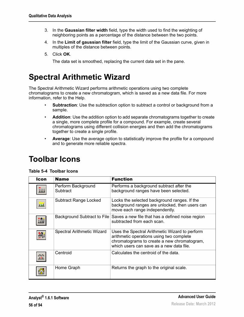
Qualitative Data Analysis
3. In the Gaussian filter width field, type the width used to find the weighting of neighboring points as a percentage of the distance between the two points.
4. In the Limit of gaussian filter field, type the limit of the Gaussian curve, given in multiples of the distance between points.
5. Click OK.
The data set is smoothed, replacing the current data set in the pane.
Spectral Arithmetic WizardThe Spectral Arithmetic Wizard performs arithmetic operations using two complete chromatograms to create a new chromatogram, which is saved as a new data file. For more information, refer to the Help.
• Subtraction: Use the subtraction option to subtract a control or background from a sample.
• Addition: Use the addition option to add separate chromatograms together to create a single, more complete profile for a compound. For example, create several chromatograms using different collision energies and then add the chromatograms together to create a single profile.
• Average: Use the average option to statistically improve the profile for a compound and to generate more reliable spectra.
Toolbar IconsTable 5-4 Toolbar Icons
Icon Name FunctionPerform Background Subtract
Performs a background subtract after the background ranges have been selected.
Subtract Range Locked Locks the selected background ranges. If the background ranges are unlocked, then users can move each range independently.
Background Subtract to File Saves a new file that has a defined noise region subtracted from each scan.
Spectral Arithmetic Wizard Uses the Spectral Arithmetic Wizard to perform arithmetic operations using two complete chromatograms to create a new chromatogram, which users can save as a new data file.
Centroid Calculates the centroid of the data.
Home Graph Returns the graph to the original scale.
Analyst® 1.6.1 Software
56 of 94
Advanced User Guide
Release Date: March 2012

Qualitative Data Analysis
Overlay Overlays graphs.
Cycle Overlays Cycles between overlaid graphs.
Sum Overlays Adds the graphs together.
Show Fragment Interpretation Tool
Opens Fragment Interpretation tool, which calculates the single, non-cyclic bond cleavage fragments from a .mol file.
Smooth Smooths data using the smooth algorithm.
Gaussian smooth Smooths data using Gaussian smoothing.
Table 5-4 Toolbar Icons (Continued)
Icon Name Function
Advanced User Guide
Release Date: March 2012Analyst® 1.6.1 Software
57 of 94

Qualitative Data Analysis
Analyst® 1.6.1 Software
58 of 94
Advanced User Guide
Release Date: March 2012
6
Quantitative Data AnalysisCalibration OptionsThe calibration options define the parameters for a calibration curve, which are used to determine the calculated concentration of the samples. The curve is a plot of the concentration of the standard against the area or height of the standard if no internal standard is used. If an internal standard is used, the curve is a plot of the concentration ratio against the area or height ratio. This curve is used, along with the area (or height) for the unknowns, to interpolate the calculated concentration.
Choose the best regression type or fit to fit the curve to the points and the best weighting factor for the project.
About Calibration CurvesThe calibration curve is used to determine the calculated concentration of samples, including QC samples. It is a curve that results from plotting the concentration of the standard versus its area or height, or ratios, if an internal standard is used. The area or height of a sample is then applied to this curve to determine the sample concentration, as displayed in the Results Table. The regression equation generated by this calibration curve is used to calculate the concentration of the unknown samples.
The software places the known concentrations (or ratios) on the x-axis and the calculated area or height (or ratios) on the y-axis. It then plots the points for all the standards in the batch. The system produces a best-fit curve to those points through regression and weighting type that is selected. This curve is used, along with the area (or height), for the unknowns to interpolate the concentration.
Select the Best Regression TypeAfter selecting a regression type (fit), the user cannot see the calibration curve from the wizard. Instead, use the preset values, experience, or corporate policy to choose a regression type.
After changing the fit, check the Accuracy column in the Results Table for changes. The better the fit is, the better the accuracy of the quantitative analysis will be.
The calibration curve plots the standards concentration against its peak area or height (or ratios, if an internal standard is used). When the points for the standards are plotted, determine the best fit for the curve to these points and indicate the choice in the Specify Calibration dialog of the wizard. The preset fit is linear, which assumes that all the standards will fall on a straight line. Select from the types of fit in Table 6-1.
Table 6-1 Types of Fit
Fit DescriptionLinear Linear regression assumes that the standard points fall on a straight
line.
Advanced User Guide
Release Date: March 2012Analyst® 1.6.1 Software
59 of 94
Quantitative Data Analysis
Choosing the Best Weighting Factor
The calibration curve plots the standards concentration against its peak area or height. When the points for the standards are plotted, determine the best weighting factor for these points and indicate it in the Specify Calibration dialog. The preset fit is None, which assumes that all points along the curve have the same importance. Select from the types of weighting in Table 6-2.
Integration AlgorithmsThe Analyst® software has two integration algorithms: the original Analyst Classic integration algorithm and the IntelliQuan integration algorithms. The IntelliQuan algorithm provides more consistent peak-finding and integrated functionality, with fewer parameters that require adjustment.
Linear Through Zero Linear Through Zero regression assumes that the standard points fall on a straight line and that the points line up with the zero point on the x- and y- axes. Use this setting to force the line to go through the zero point.
Quadratic If the standard points do not fall on a straight line, use quadratic regression to produce a quadratic fit to the data points.
Mean Response Factor If the standard points fall on a straight line, then to average the points, use mean response factor regression to produce an average of the slope for every point on the curve.
Power If there is some linear and some curvature in the line of points, use power regression instead of linear or quadratic regression to produce a line somewhere between these fits.
Table 6-2 Types of Weighting
Weighting Description1/x To place some additional emphasis on lower-value points, use a weighting
factor of 1/x.
1/x2 Use a weighting of 1/x2 to place much higher emphasis on lower-value points.
1/y Use a weighting factor of 1/y when calibrating by the area (y-axis) rather than by the concentration (x-axis), and some emphasis needs to be placed on lower-value points. A weighting of 1/y is a variant of 1/x where y and x should be proportional to each other.
1/y2 Use a weighting factor of 1/y2 when calibrating by the area (y-axis) rather than by the Concentration (x-axis), and a much higher emphasis needs to be placed on lower-value points. A weighting of 1/y squared is a variant of1/x squared where y and x should be proportional to each other.
In x Use the logarithm of x to place more emphasis on higher-value points.
In y Use the logarithm of y to place more weight on higher-value points. Use when calibrating by the area (y-axis) rather than by the concentration(x-axis).
Table 6-1 Types of Fit (Continued)
Fit Description
Analyst® 1.6.1 Software
60 of 94
Advanced User Guide
Release Date: March 2012

Quantitative Data Analysis
Analyst Classic and IntelliQuan Integration AlgorithmsThe IntelliQuan algorithm uses one of two peak-finding parameters: Automatic IQA II, which is a parameterless setting, or Specify Parameters MQ III. After integrating peaks using the IntelliQuan algorithm, choose which peak-finding parameter best fits the data set. This is done in the displayed peak integration parameters in the Peak Review pane or window.
Table 6-3 shows the parameters available with the Analyst Classic algorithm.
Table 6-4 shows the parameters available with the MQ III algorithm, but not the IQA II algorithm.
Table 6-3 Analyst Classic Algorithm
Parameter DefinitionDefault Bunching Factor The number of points to be averaged together and
considered as a single point for the purpose of peak-finding.
Default Number of Smooths The number of times to smooth the chromatogram.
Default Void Volume Retention Time
Any peaks that appear before this time are ignored.
Default Concentration Units The concentration units used to describe the sample concentration, for example, pg/µL.
Default Calculated Concentration Units
The concentration units used to describe the calculated sample concentration, for example, pg/µL.
Default RT Window The time window centered at the expected retention time for peak-finding. For example, a 30 second retention time window gives an additional 15 seconds before and after the expected retention time.
Table 6-4 MQ III Algorithm
Parameter DefinitionDefault Noise Percentage The threshold used in peak-finding. Only peaks higher than
this specified percentage will be detected.
Default Baseline Subtraction Window
A time window around each data point that is used to determine the height of the baseline correction to be applied to that point. This time window helps remove excessive noise from the chromatogram. The baseline is defined as the line connecting the point of minimum intensity on the left side of a given data point to the point of minimum intensity on the right side, within the specified window.
Default Peak-Splitting Factor Controls whether a given peak cluster consists of multiple adjacent peaks or one (possibly noisy) peak. If the intensity dip is less than the value specified, then a single peak is reported; otherwise the point with minimum intensity in the dip splits the cluster into two separate peaks. Setting a large factor will prevent clusters from being split into more than one peak.
Default Void Volume Retention Time
Any peaks that appear before this time are ignored.
Advanced User Guide
Release Date: March 2012Analyst® 1.6.1 Software
61 of 94

Quantitative Data Analysis
Table 6-5 shows the parameters available for use with both IntelliQuan algorithms.
Quantitation Method-Creation ToolsThe software offers four quantitation method-creation tools, each of which creates a fully functional method. The best choice of tool depends on the tasks to accomplish.
WizardsThere are two available method-creation wizards: the Standard Quantitation wizard and the Automatic Quantitation wizard. Both allow the user to select the batch or batches to be quantified, create or select a quantitation method, and then integrate the sample data.
The difference between the two is the type of method created. The standard wizard creates a standard method, while the automatic wizard creates an automatic method. Peaks are not verified as part of the method creation (the peaks can still be reviewed after integration has taken place).
There is only one common occasion for which peaks do not need to be verified: when quantitation is done simply to integrate, and not to find concentrations. This may need to be done, for example, for a batch that contains different compounds in every sample, or when the mass is not the same from sample to sample. If this is the case, use the automatic wizard. Otherwise, to perform quantitation, use the standard wizard.
Use the Standard Quantitation wizard after acquiring the sample to do the following:
• Choose a representative sample.
Report Largest Peak Selecting this parameter returns the largest peak in the retention time window. If this parameter is not selected, the closest peak to the expected retention time is found. The expected retention time is automatically calculated in the Quantitation Wizard.
Table 6-5 IntelliQuan Algorithm
Parameter DefinitionDefault Minimum Peak Height The minimum height of a peak required for peak integration.
Default Minimum Peak Width The minimum width of a peak required for peak integration.
Default RT Window Specifies the time window centered at the expected retention time for peak-finding. For example, a 30 second retention time window gives an additional 15 seconds before and after the expected retention time.
Default Smoothing Width The number of points used in data smoothing.
Default Concentration Units The concentration units used to describe the sample concentration, for example, pg/µL.
Default Calculated Concentration Units
The concentration units used to describe the calculated sample concentration, for example, pg/µL.
Table 6-4 MQ III Algorithm (Continued)
Parameter Definition
Analyst® 1.6.1 Software
62 of 94
Advanced User Guide
Release Date: March 2012
Quantitative Data Analysis
• Select analyte and internal standard peaks.
• Adjust peak-finding and integration parameters.
• Review peaks during method creation.
• Select calibration.
Use the Automatic Quantitation wizard to select a batch, create a method (without peak confirmation), and then integrate the sample data. This wizard is quicker than the Standard wizard and does not require that the masses scanned be the same for all samples. It does not, however, allow selecting an internal standard—all ions are treated as analytes.
Use the Automatic Quantitation wizard after acquiring the sample in the following scenarios:
• Want to select calibration.
• Do not want to adjust peak-finding and integration parameters.
• Do not want to select analyte peak names.
• Do not want any internal standards.
• Do not want to review peaks during method creation, or have different compounds in every sample.
When peaks are only being integrated, they do not need to be verified as no concentration calculation is required. In this case, use the Automatic quantitation method creation, which allows reviewing the peaks after integration has taken place.
Find Peaks Using an Automatic MethodThe software uses the standard peak-detection process, with the following exceptions:
• It uses the bunching factor and the number of smooths (from the wizard) as is.
• It calculates the expected retention time and noise and area thresholds separately for every peak.
Quantitation Method EditorUse this option after acquiring the sample to do the following:
• Adjust peak-finding and integration parameters.
• Select analyte and internal standard peaks.
• Select calibration.
Use the Quantitation Method Editor to do three additional tasks:
• Sum ions for integration.
• Use an internal standard from a different period or experiment (if the internal standard was acquired in a different period or experiment than the analyte).
• Edit an existing method.
The Semi-Automatic Method EditorThe Semi-Automatic Quantitation Method Editor is part of the Batch Editor. Use the Semi-Automatic Quantitation Method Editor to select quantitation information, such as sample type and
Advanced User Guide
Release Date: March 2012Analyst® 1.6.1 Software
63 of 94

Quantitative Data Analysis
sample concentration, prior to data acquisition. This preparation makes performing subsequent quantitative analysis easier. Alternatively, a full method can be selected in the Batch Editor, which is then automatically applied at the end of the batch run to generate the quantitation Results Table.
Use this option in the following scenarios:
• Have not yet acquired any samples.
• Want to select names and masses for analyte and internal standard peaks.
• Want to select concentrations and sample types on the Quantitation tab in the Batch Editor, but do not have any other quantitation method.
• Want to edit the quantitation method, if necessary, at a later time.
Find Peaks Using a Semi-Automatic MethodThe software uses the standard peak-detection process, with the following exceptions:
• It uses the bunching factor (from the Quantitation Method Options dialog) and the number of smooths (from the Create Semi-Automatic Quantitation Method dialog) as is.
• It uses the most concentrated standard as the representative sample. To establish a retention time, it uses the largest peak within that chromatogram.
• To set noise and area thresholds, it uses the resulting baseline noise. (This process is identical to how the preset values are set for peaks in normal methods.) These integration parameters are applied to all other samples.
• If the batch being examined does not contain quantitation information (sample type and concentrations), the retention time and thresholds are calculated separately for every peak (as for fully automatic methods).
Metric PlotsA metric plot graphically shows the data in a Results Table column plotted against the x-axis or the y-axis, or the data in two columns plotted against each other. This section describes how to generate and work with metric plots.
A few predefined metric plots are also included:
• Int_Std_Response (to locate problem sample)
• Analyte_Area versus Height (to verify chromatography behavior)
• PK profile (conc. versus time point, to run after Sample query)
Use metric plots to plot a given column, such as Analyte Peak Area, Accuracy, or Calculated Concentration, from the Results Table. Two Results Table fields can also be plotted against each other. Then points that appear outside the normal range can be investigated. Metric plots are often used with queries. For more information about queries, refer to the Help.
Generate metric plots in the following ways:
• Use the Plot button to plot a column or columns of the current Results Table, but not save the plotting criteria.
• Create a table-specific plot to save the plot criteria with the current table.
Analyst® 1.6.1 Software
64 of 94
Advanced User Guide
Release Date: March 2012

Quantitative Data Analysis
• Create a global plot to save the plotting criteria for use with future Results Tables.
QC, unknown, blanks, double blanks, or solvents cannot be seen on the calibration curve, but metric plots can be generated of them.
Generate a Metric Temporary Plot1. With a Results Table open, do one of the following:
• To plot the data on the y-axis with the x-axis as an index, click the heading of the column for the data to be plotted.
• To plot the data from the first selected column on the x-axis and the second selected column on the y-axis, select two columns by pressing the Ctrl key and clicking the column headings.
2. Above the Results Table, click the Metric Plot by Selection icon.
The metric plot opens.
3. Right-click in the plot pane and then click Data Legend to view an explanation of the colors used by the plot.
4. Right-click in the plot pane and then click Point Legend to view an explanation of the symbols used by the plot.
Generate a Metric Plot and Save the Plot Criteria1. Open the Tutorial Results Table.rdb Results Table.
2. Right-click in the Results Table and then click Metric Plot > New.
Figure 6-1 Example of a metric plot
Item Description1 Double blanks
1
Advanced User Guide
Release Date: March 2012Analyst® 1.6.1 Software
65 of 94
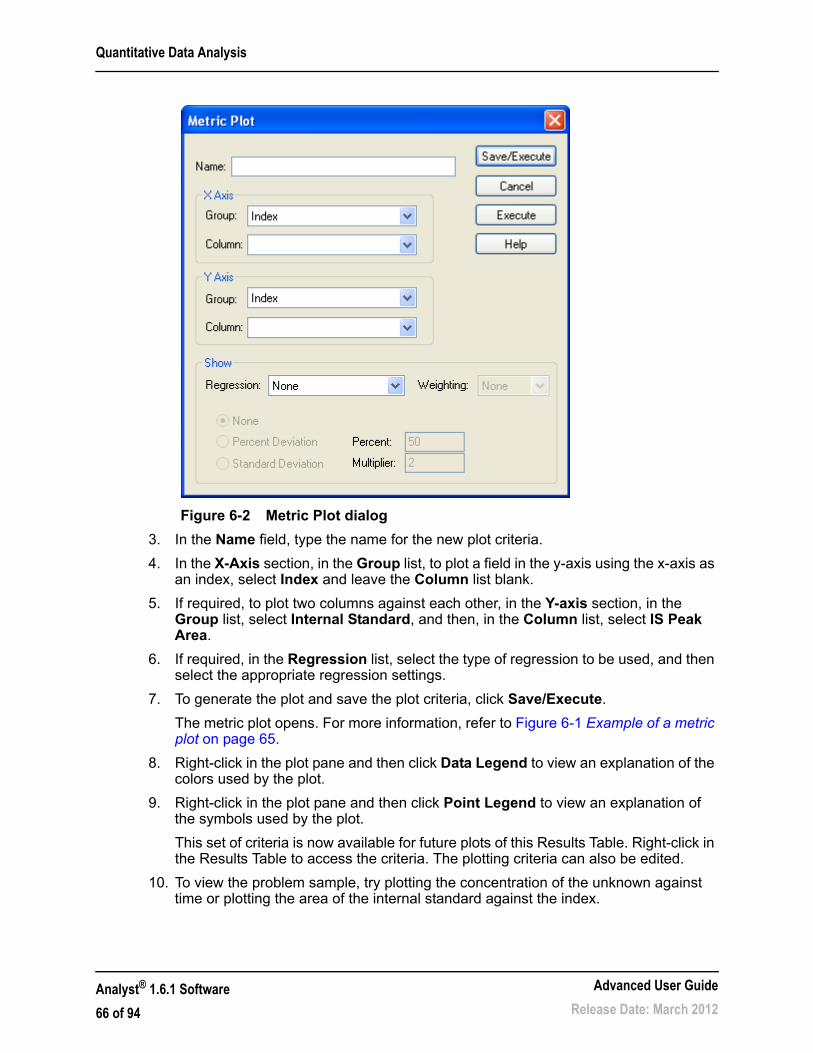
Quantitative Data Analysis
Figure 6-2 Metric Plot dialog
3. In the Name field, type the name for the new plot criteria.
4. In the X-Axis section, in the Group list, to plot a field in the y-axis using the x-axis as an index, select Index and leave the Column list blank.
5. If required, to plot two columns against each other, in the Y-axis section, in the Group list, select Internal Standard, and then, in the Column list, select IS Peak Area.
6. If required, in the Regression list, select the type of regression to be used, and then select the appropriate regression settings.
7. To generate the plot and save the plot criteria, click Save/Execute.
The metric plot opens. For more information, refer to Figure 6-1 Example of a metric plot on page 65.
8. Right-click in the plot pane and then click Data Legend to view an explanation of the colors used by the plot.
9. Right-click in the plot pane and then click Point Legend to view an explanation of the symbols used by the plot.
This set of criteria is now available for future plots of this Results Table. Right-click in the Results Table to access the criteria. The plotting criteria can also be edited.
10. To view the problem sample, try plotting the concentration of the unknown against time or plotting the area of the internal standard against the index.
Analyst® 1.6.1 Software
66 of 94
Advanced User Guide
Release Date: March 2012
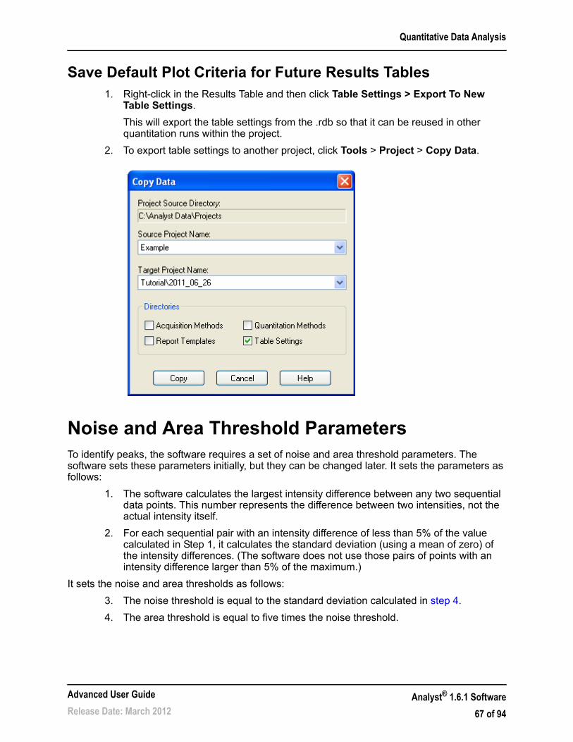
Quantitative Data Analysis
Save Default Plot Criteria for Future Results Tables1. Right-click in the Results Table and then click Table Settings > Export To New
Table Settings.
This will export the table settings from the .rdb so that it can be reused in other quantitation runs within the project.
2. To export table settings to another project, click Tools > Project > Copy Data.
Noise and Area Threshold ParametersTo identify peaks, the software requires a set of noise and area threshold parameters. The software sets these parameters initially, but they can be changed later. It sets the parameters as follows:
1. The software calculates the largest intensity difference between any two sequential data points. This number represents the difference between two intensities, not the actual intensity itself.
2. For each sequential pair with an intensity difference of less than 5% of the value calculated in Step 1, it calculates the standard deviation (using a mean of zero) of the intensity differences. (The software does not use those pairs of points with an intensity difference larger than 5% of the maximum.)
It sets the noise and area thresholds as follows:
3. The noise threshold is equal to the standard deviation calculated in step 4.
4. The area threshold is equal to five times the noise threshold.
Advanced User Guide
Release Date: March 2012Analyst® 1.6.1 Software
67 of 94
Quantitative Data Analysis
Recalculate the Noise and Area ThresholdIf a new background area is defined, the software recalculates the noise and area thresholds as follows. For each sequential pair of data points, the software calculates the standard deviation, using a mean of zero, of the intensity difference. The Analyst software uses all points within the selected range because it is explicitly being told that the selected area is background noise.
It sets the noise and area thresholds as follows:
1. The noise threshold is equal to the standard deviation calculated for the selected range.
2. The area threshold is equal to five times the noise threshold.
Peak IntegrationThe following are integration types by which the baseline was found and integrated when the peak was found.
• Manual: The peak was manually integrated by the user.
• Automatic: The peak was automatically integrated as follows:
• Baseline-to-baseline: The peak area is defined by vertical droplines at the beginning and end of the peak which extend to the baseline. This integration type is possible only for peaks that do not have another peak immediately preceding or following.
• Valley: Same as baseline-to-baseline, except that it applies only to peaks that do have another peak immediately preceding or following.
• Exponential Skim: The peak area is the main or parent peak in an exponential skim.
• Exponential Child: The peak area is the child peak resulting in an exponential skim.
Peak ReviewDuring peak review users can survey the peaks that the software selected and then redefine the peak or the start and end points where necessary.
In general, the software is adept at accurately identifying analyte and internal standard peaks. For a variety of reasons, including sample acquisition and quantitation method definition, sometimes the software misses the correct peak, chooses the wrong one, or is unable to locate a
Note: The minimum value for both the noise and area thresholds is 0.000001. If the calculations produce a value that is lower than this minimum, then the software resets the value of that threshold at 0.000001.
Note: The minimum value for both the noise and area thresholds is 0.000001. If the calculations produce a value that is lower than this minimum, then the software resets the value of that threshold at 0.000001.
Analyst® 1.6.1 Software
68 of 94
Advanced User Guide
Release Date: March 2012
Quantitative Data Analysis
peak at all. Other times, although the software may correctly identify the peak, users may not agree with the start or end points selected.
Peak Review Tips
Detect PeaksThe software detects peaks in four stages.
1. First, it finds the potential peak start by examining the distance between each bunched point and the preceding one. When the distance exceeds the current noise threshold, a potential peak start has been found.
2. Then it confirms the peak start by making sure that enough points exist in a row to exceed the area threshold.
3. Next, it finds the peak top by searching for a point that is lower than the previous point.
4. Finally, it finds the end of the peak by identifying the place where the distance between one bunched point and the next falls below the noise threshold. If necessary, it then separates peaks.
Table 6-6 Peak Review Tips
To do this... ... do thisPeak Integration: To review peaks
To review all peaks, make sure that all samples are listed in the Results Table.
The Peak Review window contains the peaks listed in the Results table. If some samples are hidden in the table (for example, if a query is applied), then they are also hidden in peak review.
Peak Integration: To move to the first peak in the batch
Right-click anywhere in the Peak Review pane and then click Show First Page. To move to the last peak in the batch, right-click anywhere in the Peak Review pane and then click Show Last Page.
Advanced User Guide
Release Date: March 2012Analyst® 1.6.1 Software
69 of 94
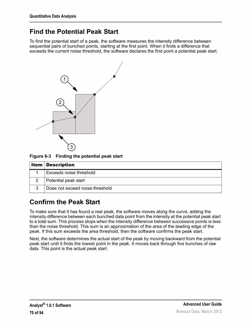
Quantitative Data Analysis
Find the Potential Peak StartTo find the potential start of a peak, the software measures the intensity difference between sequential pairs of bunched points, starting at the first point. When it finds a difference that exceeds the current noise threshold, the software declares the first point a potential peak start.
Confirm the Peak StartTo make sure that it has found a real peak, the software moves along the curve, adding the intensity difference between each bunched data point from the intensity at the potential peak start to a total sum. This process stops when the intensity difference between successive points is less than the noise threshold. This sum is an approximation of the area of the leading edge of the peak. If this sum exceeds the area threshold, then the software confirms the peak start.
Next, the software determines the actual start of the peak by moving backward from the potential peak start until it finds the lowest point in the peak. It moves back through five bunches of raw data. This point is the actual peak start.
Figure 6-3 Finding the potential peak start
Item Description1 Exceeds noise threshold
2 Potential peak start
3 Does not exceed noise threshold
1
2
3
Analyst® 1.6.1 Software
70 of 94
Advanced User Guide
Release Date: March 2012

Quantitative Data Analysis
Find the Peak TopTo find the peak top, the software first looks for a point that is lower than the preceding point. Then, to confirm that it has found the top correctly, it sums the intensity differences between the potential top and subsequent bunched points until it reaches the end of the peak. If the total distance between points exceeds two-thirds of the area threshold, then the peak top is confirmed. That is, the software makes sure it has a peak first, and then works backward to find the top of it.
Figure 6-4 Confirming the peak start
Item Description1 Sum of area slices greater than threshold
Figure 6-5 Confirming the actual peak start
Item Description1 Look through data points in this region
2 Minimum data point
3 Potential peak start
1
3
2
1
Advanced User Guide
Release Date: March 2012Analyst® 1.6.1 Software
71 of 94

Quantitative Data Analysis
If, however, the software finds a higher bunched point before the area test has been passed, then it identifies a new top and restarts the area test.
Note: The actual retention time for a peak is not simply the point identified as described previously. Instead, it is determined from a quadratic fit based on the three highest data points.
Figure 6-6 Finding the peak top
Item Description1 Sum of area slices is greater than two thirds of the area threshold
Figure 6-7 Identifying a new peak top
Item Description1 The shoulder has a maximum, but the cumulative crest area is not greater than two
thirds of the area threshold
1
1
Analyst® 1.6.1 Software
72 of 94
Advanced User Guide
Release Date: March 2012

Quantitative Data Analysis
Find the Peak EndThe software declares a peak end point when one of the following occurs:
• The difference between two consecutive points fails the noise threshold test.
• The software detects the start of a new peak.
In either case, the lowest bunched point from the last five bunches is considered to be the actual end point of the peak.
In general, the software finds several peaks for each chromatogram. The peak it selects is the one whose retention time is the closest to the expected retention time, specified in the method. If no peak has a retention time within the specifications, the software marks the peak as not found.
Figure 6-8 Finding peaks
Item Description1 The shoulder has no separate maximum point
1
1
2
3
Advanced User Guide
Release Date: March 2012Analyst® 1.6.1 Software
73 of 94
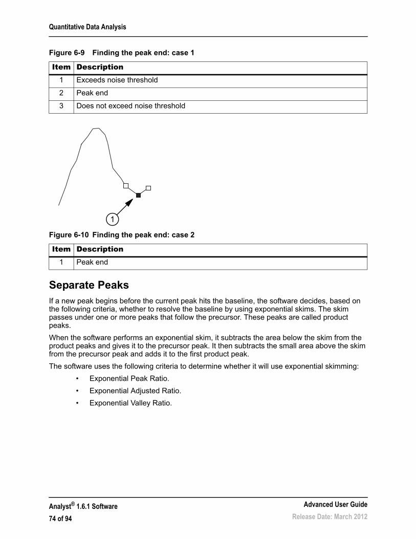
Quantitative Data Analysis
Separate PeaksIf a new peak begins before the current peak hits the baseline, the software decides, based on the following criteria, whether to resolve the baseline by using exponential skims. The skim passes under one or more peaks that follow the precursor. These peaks are called product peaks.
When the software performs an exponential skim, it subtracts the area below the skim from the product peaks and gives it to the precursor peak. It then subtracts the small area above the skim from the precursor peak and adds it to the first product peak.
The software uses the following criteria to determine whether it will use exponential skimming:
• Exponential Peak Ratio.
• Exponential Adjusted Ratio.
• Exponential Valley Ratio.
Figure 6-9 Finding the peak end: case 1
Item Description1 Exceeds noise threshold
2 Peak end
3 Does not exceed noise threshold
Figure 6-10 Finding the peak end: case 2
Item Description1 Peak end
1
Analyst® 1.6.1 Software
74 of 94
Advanced User Guide
Release Date: March 2012

Quantitative Data Analysis
QueriesA query is a method of selecting only those records that meet certain criteria. Users can use queries to view particular parts of the data in the Results Table that interests them, based on textual or mathematical selections.
When a query is used, the table displays only the rows of data that meet the selected criteria. All columns are displayed. Selections can be further refined by running a second query on the rows displayed by the first query.
Use pre-defined choices and typed entries to create a query that can be executed, saved, or modified. Each line of the query works like a Boolean search that runs against Results Table columns to determine which records to display. Each line of the query selects only the records for display that meet its criteria. A preset or table-specific query can be defined.
Queries on Sample TypeFor a query designed to select only the standard sample type, the Results Table displays only those rows of data that contain Standard in the Sample Type column.
Default Queries and Table-Specific QueriesA default query is generally used to identify samples that do not meet certain criteria. A table-specific query is generally used to identify records that meet certain criteria.
The default query is generally used to find problems with quality control or standards. If the concentration and maximum variation of the QCs and standards are selected in the Quantitation
Figure 6-11 Separating peaks: an exponential skim
Item Description1 This area is subtracted from the precursor peak and added to the first product peak
2 Exponential skim
3 Cluster baseline
4 These areas are subtracted from the product peaks and added to the precursor peaks
1
3
2
4 4
Advanced User Guide
Release Date: March 2012Analyst® 1.6.1 Software
75 of 94

Quantitative Data Analysis
Method Wizard, then the Results Table displays only those samples that lie outside this range. If the Results Table displays nothing, then the samples are all right.
Table-specific queries are run against a displayed Results Table to select records that meet certain criteria. Design these queries through the menu that is available by right-clicking in the table. Save and export a query to make it available for future Results Tables.
Table-Specific or Global Settings
When working with table setting options, procedures can be table-specific or global.
• Table-specific settings: When table settings are modified on a table itself, the changes to the settings are available only to that table; however, they can be exported as global settings.
• Global settings: Modifying global settings involves making changes to a group of settings that can be applied to future Results Tables. To customize a Results Table that is being created, choose a group of settings on the Create Quantitation Set: Select Settings & Query page. If a group of settings is not selected, the software automatically uses the preset settings.
How Accuracy Variations Affect the ResultsFor preset queries, accuracy is expressed as a percent and implemented as plus or minus that number. For example, if 10 is typed for Maximum Variation for standards in the Create Default Query dialog, then all records containing standards whose accuracy falls outside 90% and 110% are displayed in the Results Table. If 5 is typed, only standards whose accuracy is less than 95% and greater than 105% would appear in the Results Table. For more information, refer to Results Tables on page 82.
RegressionThis section gives the equations for each of the regression types. In the following equations, x, y, and w are as described in Weighting Factors on page 94.
In the following equations, x represents the analyte concentration for standard sample types, and y represents the corresponding peak area or height. The exact variables used for the regression depend on whether or not an internal standard is being used and whether the peak area or the peak height is used as shown in the following table.
Where:
• Ca = actual analyte concentration
• Cis = internal standard concentration
Table 6-7 Regression Formulae
Internal Standard Used? Area Used? x yYes Yes Ca/Cis/DF Aa/Ais
Yes No Ca/Cis/DF Ha/His
No Yes Ca/DF Aa
No No Ca/DF Ha
Analyst® 1.6.1 Software
76 of 94
Advanced User Guide
Release Date: March 2012

Quantitative Data Analysis
• DF = dilution factor
• Aa = analyte peak area
• Ais = internal standard peak area
• Ha = analyte peak height
• His = internal standard peak height
Linear RegressionLinear regression assumes that the points of the standard fall on a straight line.
The linear calibration equation is calculated as:
y = m x + b
The slope and intercept are calculated as:
The correlation co-efficient is calculated as:
where:
Linear Through Zero RegressionLinear through zero regression assumes that the points of the standard fall on a straight line and that the points do line up with the zero point on the x and y axes. Use this setting to force the line to go through the zero point.
The linear through zero calibration equation is calculated as:
y = m x
The slope is calculated as:
The correlation co-efficient is calculated as:
If the standard points fall on a straight line, then to average the points use mean response factor regression to produce an average of the slope for every point on the curve.
Mean Response FactorThe mean response factor calibration is calculated as:
y = m x
m wwxy wxwy– Dx=
b wx2wy wxwxy– Dx=
r wwxy wxwy– DxDy =
Dx wwx2 wx 2–=
Dy wwy2 wy 2–=
m wxy wx2=
r wxy wx2wy2 =
Advanced User Guide
Release Date: March 2012Analyst® 1.6.1 Software
77 of 94
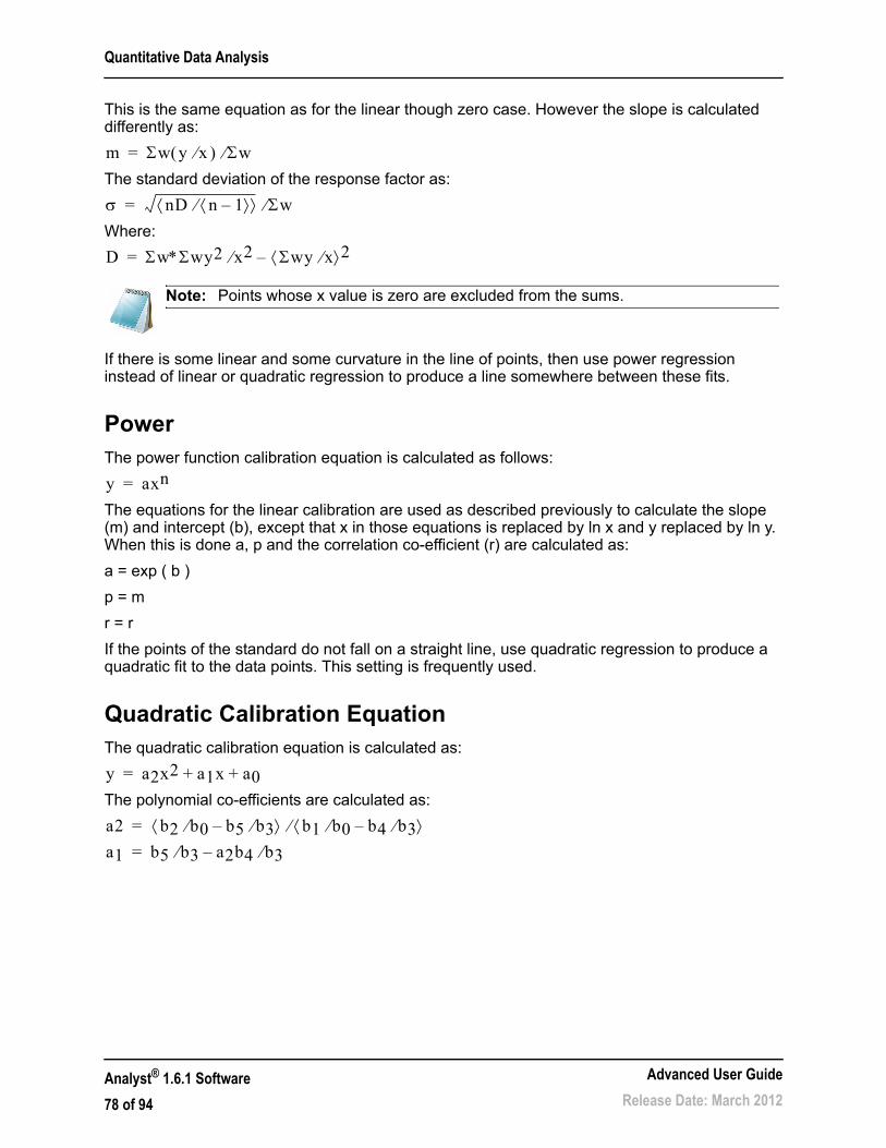
Quantitative Data Analysis
This is the same equation as for the linear though zero case. However the slope is calculated differently as:
The standard deviation of the response factor as:
Where:
If there is some linear and some curvature in the line of points, then use power regression instead of linear or quadratic regression to produce a line somewhere between these fits.
PowerThe power function calibration equation is calculated as follows:
The equations for the linear calibration are used as described previously to calculate the slope (m) and intercept (b), except that x in those equations is replaced by ln x and y replaced by ln y. When this is done a, p and the correlation co-efficient (r) are calculated as:
a = exp ( b )
p = m
r = r
If the points of the standard do not fall on a straight line, use quadratic regression to produce a quadratic fit to the data points. This setting is frequently used.
Quadratic Calibration EquationThe quadratic calibration equation is calculated as:
The polynomial co-efficients are calculated as:
Note: Points whose x value is zero are excluded from the sums.
m w y x w=
nD n 1– w=
D wwy2 x2 wy x 2–=
y axn=
y a2x2 a1x a0+ +=
a2 b2 b0 b5 b3– b1 b0 b4 b3– =
a1 b5 b3 a2b4 b3–=
Analyst® 1.6.1 Software
78 of 94
Advanced User Guide
Release Date: March 2012

Quantitative Data Analysis
The correlation co-efficient as:
Where:
Report TemplatesAdd the following information to report headers and footers.
Tip! Make a backup of the existing report templates before editing them.
Table 6-8 Basic Design Elements
Element DefinitionPrinting Date The date the document was printed.
Printing Time The time the document was printed.
Operator The operator who printed the document.
Workstation The workstation from which the document was printed from.
Page n of N Indicates the page number of total number of pages.
Custom Field Create custom text here.
Analyst Version Indicates the version of the Analyst® software.
User Type Indicates the user type (Security).
Electronic Signature Indicates whether the electronic signature feature (security) is enabled or disabled.
Table 6-9 Acquisition Elements
Element DefinitionAcquisition File The name of the data file with the sample acquisition information.
Acquisition Date The date the sample acquisition was run.
Acquisition Time The time of the sample acquisition was run.
Operator The name of the operator who ran the sample batch.
a0 wy a1wx– a2wx2– w=
r 1 ww y a2x2– a1x– a0– 2 Dy– =
Dy wwy2 wy 2–=
b0 wx w wx2 wx–=
b1 wx2 w wx3 wx–=
b2 wy w wxy wx–=
b3 wx2 wx wx3 wx2–=
b4 wx3 wx wx4 wx2–=
b5 wxy wx wx2y wx2–=
Advanced User Guide
Release Date: March 2012Analyst® 1.6.1 Software
79 of 94

Quantitative Data Analysis
Batch Name The name of the batch.
Sample Number The number related to the sample.
Sample Name The name of the sample.
Sample Comment Shows any comments about the sample entered through the Acquisition Method Editor.
Sample ID The identification number of the sample.
Scan Mode Indicates the method in which the system calculates the mass points for a scan for a full mass range scan.
Scan Type and Polarity Indicates the acquisition scan type (Q1, Q3, MRM, Product ion, Precursor ion, neutral loss/gain) and acquisition method polarity (positive or negative).
Scan Mass(es) Ions or ion fragments to be scanned.
Dwell Time The time the system takes to scan a particular mass.
Pause Time Indicates the pause between the scanning of mass ranges or between experiments.
Ion Energy Ion energy comes from the acquisition method and is related to the IonSpray™ ion source voltage or the collision energy.
Collision Energy Collision energy comes from the acquisition method and is related to the IonSpray ion source voltage.
Period and Experiment A period contains a collection of experiments; an experiment contains a number of properties, such as Scan Type, Scan Mode, Resolution, Ion Source Parameters, and a collection of mass ranges or masses.
State Table Parameters The instrument parameters used in the experiment.
Pump The name of the pump used for the experiment.
Autosampler The name of the autosampler used for the experiment.
Custom Annotation The custom text added via the Batch Editor.
Collected By The name of the person who collected the data.
Table 6-10 Quantitation Elements
Element DefinitionResults Table Name The name of the Results Table.
Results Table Path The location of the Results Table.
Method Name The name of the quantitation method.
Method Path The location of the method file.
Project Name The name of the project.
Results Table Name The name of the Results Table.
Table 6-9 Acquisition Elements (Continued)
Element Definition
Analyst® 1.6.1 Software
80 of 94
Advanced User Guide
Release Date: March 2012

Quantitative Data Analysis
Customize ReportsThe Report Template Editor provides a way to customize reports by setting up headers, footers, and page layouts. Use report templates with both printed output and data exported to another application.
Printed output includes several types of elements.
• Window: Windows in the Analyst software appear in the working area of the software window, below the toolbar and to the right of the Navigation bar. Printing a window will print everything that is shown in that space.
• Pane: Panes are parts of a window arranged in such a way that they do not overlap and are always fully visible. For example, the Method Editor window contains two panes: the Browser pane and the Method Editor pane. Information from each pane in the window can be printed.
• Report: Reports are structured sets of information created in the software. Some reports can be directly printed, such as calibration reports; other information must be exported, such as batches and quantitation Results Tables.
• Workspace: A workspace is a particular arrangement of windows and panes along with an associated file or files. Printing a workspace involves printing each open window and pane in the current mode.
Preview, Print, and Export ReportsAcquisition methods, batches, quantitation Results Tables, and graph Results Tables can be exported as reports. Other forms of information, such as calculator data, can be exported but cannot be customized with a report template.
Most areas seen on the screen can be printed. Graphs can be previewed, scaled, or copied using the Print Preview feature.
An exported report is saved in a file format that is appropriate for programs such as Notepad, Microsoft Word or Excel, or certain LIMS (Laboratory Information Management System) software.
Export reports in the following formats:
• .csv
• .doc
• .txt
The formats available depend on the information being exported. For example, a graph can be exported as a .pdf; a table of data can be exported as a .txt file.
To include additional information in the header and footer of the report, print the report using an appropriate template.
Table 6-11 Previewing, Printing, and Exporting Reports
To do this... ...do thisPreview a graph 1. Click File > Print Preview > Pane.
2. Edit the Print Preview dialog.3. Click Print.
Advanced User Guide
Release Date: March 2012Analyst® 1.6.1 Software
81 of 94
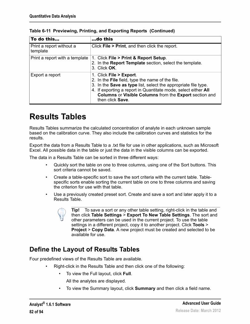
Quantitative Data Analysis
Results TablesResults Tables summarize the calculated concentration of analyte in each unknown sample based on the calibration curve. They also include the calibration curves and statistics for the results.
Export the data from a Results Table to a .txt file for use in other applications, such as Microsoft Excel. All possible data in the table or just the data in the visible columns can be exported.
The data in a Results Table can be sorted in three different ways:
• Quickly sort the table on one to three columns, using one of the Sort buttons. This sort criteria cannot be saved.
• Create a table-specific sort to save the sort criteria with the current table. Table-specific sorts enable sorting the current table on one to three columns and saving the criterion for use with that table.
• Use a previously created preset sort. Create and save a sort and later apply it to a Results Table.
Define the Layout of Results TablesFour predefined views of the Results Table are available.
• Right-click in the Results Table and then click one of the following:
• To view the Full layout, click Full.
All the analytes are displayed.
• To view the Summary layout, click Summary and then click a field name.
Print a report without a template
Click File > Print, and then click the report.
Print a report with a template 1. Click File > Print & Report Setup.2. In the Report Template section, select the template.3. Click OK.
Export a report 1. Click File > Export.2. In the File field, type the name of the file.3. In the Save as type list, select the appropriate file type.4. If exporting a report in Quantitate mode, select either All
Columns or Visible Columns from the Export section and then click Save.
Tip! To save a sort or any other table setting, right-click in the table and then click Table Settings > Export To New Table Settings. The sort and other parameters can be used in the current project. To use the table settings in a different project, copy it to another project. Click Tools > Project > Copy Data. A new project must be created and selected to be available for use.
Table 6-11 Previewing, Printing, and Exporting Reports (Continued)
To do this... ...do this
Analyst® 1.6.1 Software
82 of 94
Advanced User Guide
Release Date: March 2012

Quantitative Data Analysis
• To view the Analyte layout, click Analyte and then click a single analyte if more than one analyte exists.
• To view the Analyte Group layout, click Analyte Group and then click an analyte group.
The table opens with the selected layout.
Sort Data in Results Tables1. Select up to three columns in the Results Table in the order they need to be sorted.
2. Do one of the following:
• To sort in ascending order, click A-Z.
• To sort in descending order, click Z-A.
Sort a Results Table and Save the Sort Criteria 1. Right-click in the Results Table and then click Sort > New.
Figure 6-12 Sort dialog
2. In the Name field, type the name for the new sort.
Tip! A new analyte group must be created first. To do this, right-click in the Results Table and then click Analyte Group > New.
Tip! To go back to the full view, right-click and click Full.
Advanced User Guide
Release Date: March 2012Analyst® 1.6.1 Software
83 of 94

Quantitative Data Analysis
3. For each sorting rule to be set, in the Sort By section, do the following:
i. In the Group list, select the type of column.ii. In the Column list, select the column.iii. Select the direction of the sort: Ascending or Descending.
4. Do one of the following:
• To perform the sort, save the sort criteria, and close the Sort dialog, click Save/Execute.
• To perform the sort and close the Sort dialog without saving the sort criteria, click Execute.
Save Default Sort Criteria for Future Results Tables1. Click Tools > Settings > New Quantitation Results Table Settings.
Figure 6-13 Table Settings dialog
2. Expand the Table Settings folder and then double-click the Default folder.
3. From the expanded Default folder, select the Sorts folder.
4. Click New.
Analyst® 1.6.1 Software
84 of 94
Advanced User Guide
Release Date: March 2012

Quantitative Data Analysis
Figure 6-14 Sort dialog
5. In the Name field, type a name.
6. For each sorting rule to be set, in the Sort By section, do the following:
i. In the Group list, select the type of column.ii. In the Column list, select the column.iii. Select the direction of the sort: Ascending or Descending.
7. To save the criteria and close the Sort dialog, click OK.
8. Click Done.
Sort a Results Table using Preset Sort Criteria• Right-click in the Results Table, click Sort and then select the name of the sort.
About using Queries with Results TablesA query is a request for records in a Results Table that the certain conditions set using textual or mathematical selection criteria. Apply a query either during the process of generating a Results Table or after one has been generated. These two types of queries are called default and table-specific queries. For more information, refer to Default Queries and Table-Specific Queries on page 75.
Compare Results Between BatchesWhen more than one Results Table is displayed, obtain statistical information about the standards and QCs for additional batches in the Statistics window. Normally results are
Advanced User Guide
Release Date: March 2012Analyst® 1.6.1 Software
85 of 94

Quantitative Data Analysis
compared between batches to look for trends in the standards or QCs or to verify that the method is valid.
For two or more open Results Tables, compare results in the Statistics window. Both sets of statistics appear in the Statistics window.
How Concentration Levels Affect ResultsThe concentration is defined for all QCs and standards. If there is a change in the accuracy of the concentration level by more than the amount defined in the Max. Variation field in the Create Default Query dialog, then this information is shown in the Results Table.
Results Table LayoutsThe software has four predefined views of the Results Table.
• Full Layout View
• Summary Layout View
• Analyte Layout View
• Analyte Group Layout View
Each analyte from a multiple analytes sample can be seen in the Analyte Layout view. The preset view is Full layout.
Full Layout View
The preset Full Layout view shows the data for all analytes in the quantitation batch. The columns that are displayed depend on the columns selected in the Results Table Columns dialog, and the settings selected on the second page of the Quantitation Method Wizard.
Figure 6-15 Sample Full Layout view
Note: The number of analytes and the number of analyte names must be the same for the data to be combined in the Statistics window.
Analyst® 1.6.1 Software
86 of 94
Advanced User Guide
Release Date: March 2012
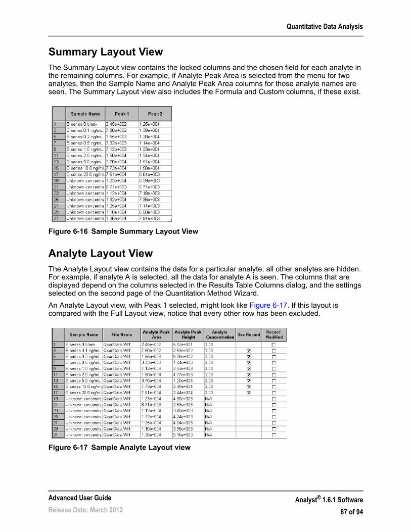
Quantitative Data Analysis
Summary Layout ViewThe Summary Layout view contains the locked columns and the chosen field for each analyte in the remaining columns. For example, if Analyte Peak Area is selected from the menu for two analytes, then the Sample Name and Analyte Peak Area columns for those analyte names are seen. The Summary Layout view also includes the Formula and Custom columns, if these exist.
Figure 6-16 Sample Summary Layout View
Analyte Layout ViewThe Analyte Layout view contains the data for a particular analyte; all other analytes are hidden. For example, if analyte A is selected, all the data for analyte A is seen. The columns that are displayed depend on the columns selected in the Results Table Columns dialog, and the settings selected on the second page of the Quantitation Method Wizard.
An Analyte Layout view, with Peak 1 selected, might look like Figure 6-17. If this layout is compared with the Full Layout view, notice that every other row has been excluded.
Figure 6-17 Sample Analyte Layout view
Advanced User Guide
Release Date: March 2012Analyst® 1.6.1 Software
87 of 94
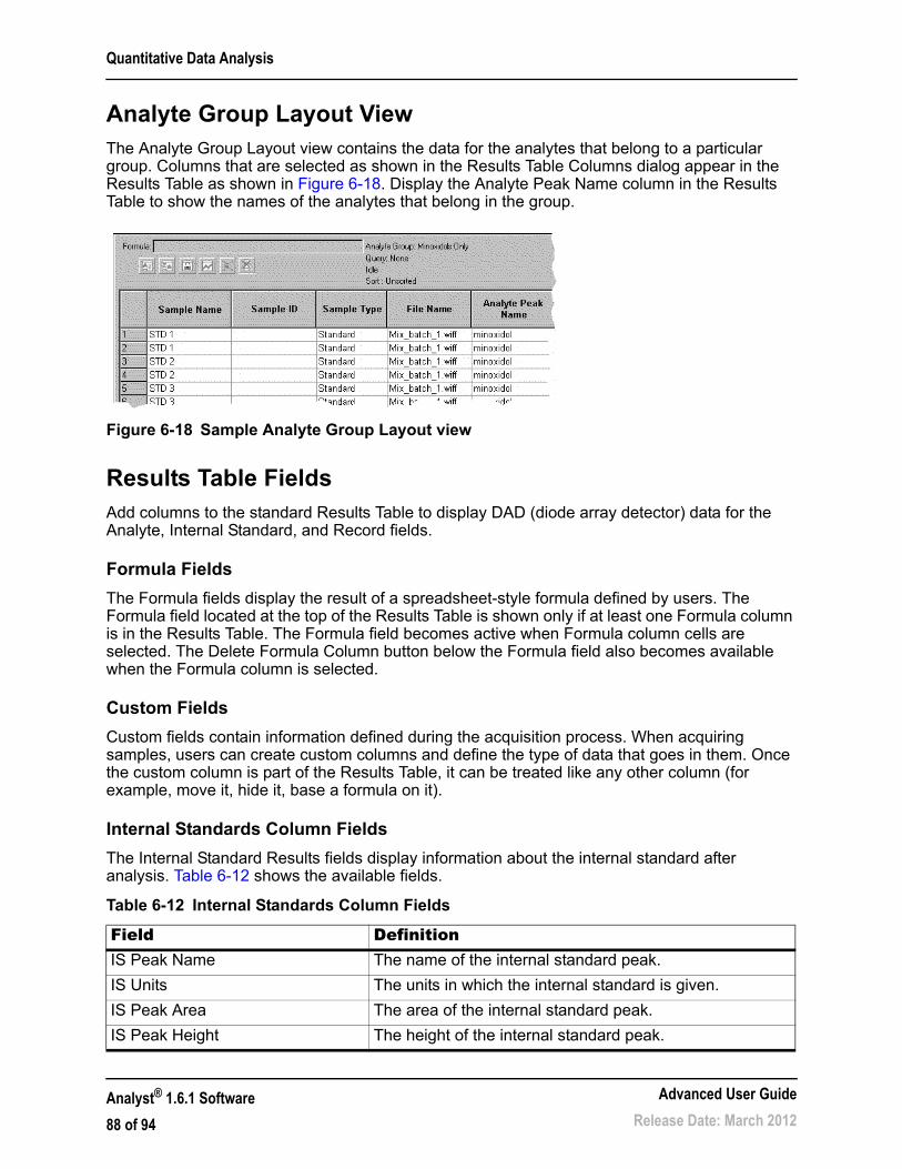
Quantitative Data Analysis
Analyte Group Layout ViewThe Analyte Group Layout view contains the data for the analytes that belong to a particular group. Columns that are selected as shown in the Results Table Columns dialog appear in the Results Table as shown in Figure 6-18. Display the Analyte Peak Name column in the Results Table to show the names of the analytes that belong in the group.
Figure 6-18 Sample Analyte Group Layout view
Results Table FieldsAdd columns to the standard Results Table to display DAD (diode array detector) data for the Analyte, Internal Standard, and Record fields.
Formula Fields
The Formula fields display the result of a spreadsheet-style formula defined by users. The Formula field located at the top of the Results Table is shown only if at least one Formula column is in the Results Table. The Formula field becomes active when Formula column cells are selected. The Delete Formula Column button below the Formula field also becomes available when the Formula column is selected.
Custom Fields
Custom fields contain information defined during the acquisition process. When acquiring samples, users can create custom columns and define the type of data that goes in them. Once the custom column is part of the Results Table, it can be treated like any other column (for example, move it, hide it, base a formula on it).
Internal Standards Column Fields
The Internal Standard Results fields display information about the internal standard after analysis. Table 6-12 shows the available fields.
Table 6-12 Internal Standards Column Fields
Field DefinitionIS Peak Name The name of the internal standard peak.
IS Units The units in which the internal standard is given.
IS Peak Area The area of the internal standard peak.
IS Peak Height The height of the internal standard peak.
Analyst® 1.6.1 Software
88 of 94
Advanced User Guide
Release Date: March 2012

Quantitative Data Analysis
IS Concentration The known concentration of the internal standard, this applies to standard and quality control sample types. Zeroes are displayed for solvent, blank, and double blank sample types; N/A is displayed for unknowns.
IS Retention Time The chromatographic retention time as determined by the software.
IS Expected Retention Time The retention time of the representative sample. Taken from the quantitation method.
IS Retention Time Window The retention time window as specified in the quantitation method.
IS Centroid Location The intensity-weighted average retention time for the analyte. The peak areas up to and after this time are identified.
IS Start Scan The cycle number associated with the period/experiment combination where the peak begins.
IS Start Time The time associated with the period/experiment combination where the peak begins.
IS Stop Scan The cycle number associated with the period/experiment combination where the peak ends.
IS Stop Time The time associated with the period/experiment combination where the peak ends.
IS Integration Type The method by which the baseline was found and integrated when the peak was found. The types are: manual, automatic (Baseline-to-Baseline, Valley, Exponential Skim, and Exponential Child).
IS Signal to Noise The signal-to-noise ratio of the peak.
IS Peak Width The ratio of the peak height to its width.
IS UV Range The UV range of the internal standard.
IS UV Channel The UV channel of the internal standard.
IS Peak Width at 50 Percent (min.) A read-only column displaying the peak width at 50% of peak height.
IS Baseline Slope (%/min.) A read-only column displaying the slope of the baseline.
IS Peak Asymmetry A read-only column displaying the peak asymmetry which is calculated by the following formula:
[(Peak End Time) – (Retention Time)] / [(Retention Time) – (Peak Start Time)]
Values near 1.0 indicate symmetric peaks, values greater than 1.0 indicate tailing peaks, and values less than 1.0 indicate fronting peaks.
IS Processing Alg A read-only column displaying the processing algorithm used.
Table 6-12 Internal Standards Column Fields (Continued)
Field Definition
Advanced User Guide
Release Date: March 2012Analyst® 1.6.1 Software
89 of 94

Quantitative Data Analysis
Record Fields
The Record fields display additional information about each sample record (information that is applicable only to the analyte, not the internal standard). Table 6-13 shows the available fields.
Sample Column Fields
The Analyte Results fields display information about each analyte and internal standard (if one was used) after analysis. Table 6-14 shows the available fields.
IS Integration Quality The Integration Quality™ Index indicates how well the peak is integrated. Values closer to 1 indicate well-integrated peaks and values closer to 0 indicate poorly integrated peaks.
Table 6-13 Record Fields
Field DefinitionUse Record Indicates whether this record should be included for calibration.
Applies to standards and QCs. If the check box is cleared, then the unused standards and QCs are struck out in the Statistics Table.
Record Modified Indicates whether the quantitation method used for the record was modified in any way from the original.
Calculated Concentration The calculated concentration of the analyte as calculated using the calibration curve.
Relative Retention Time The ratio of the retention times of the internal standard and the analyte.
Accuracy The calculated concentration divided by the known concentration (as a percentage).
Response Factor The peak area or height (depending on the regression option) divided by the analyte concentration.
Table 6-14 Results Tables: Sample Column Fields
Field DefinitionAnalyte Peak Name The name of the analyte.
Analyte Units The units in which the analyte concentrations are given.
Analyte Peak Area The area of the analyte.
Analyte Peak Height The height of the analyte peak.
Analyte Concentration The actual, known concentration of the analyte, this applies to standard and quality control sample types. Zeroes are displayed for solvent, blank, and double blank sample types; N/A is displayed for unknowns.
Analyte Retention Time The chromatographic retention time as determined by the software.
Table 6-12 Internal Standards Column Fields (Continued)
Field Definition
Analyst® 1.6.1 Software
90 of 94
Advanced User Guide
Release Date: March 2012
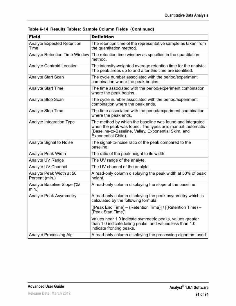
Quantitative Data Analysis
Analyte Expected Retention Time
The retention time of the representative sample as taken from the quantitation method.
Analyte Retention Time Window The retention time window as specified in the quantitation method.
Analyte Centroid Location The intensity-weighted average retention time for the analyte. The peak areas up to and after this time are identified.
Analyte Start Scan The cycle number associated with the period/experiment combination where the peak begins.
Analyte Start Time The time associated with the period/experiment combination where the peak begins.
Analyte Stop Scan The cycle number associated with the period/experiment combination where the peak ends.
Analyte Stop Time The time associated with the period/experiment combination where the peak ends.
Analyte Integration Type The method by which the baseline was found and integrated when the peak was found. The types are: manual, automatic (Baseline-to-Baseline, Valley, Exponential Skim, and Exponential Child).
Analyte Signal to Noise The signal-to-noise ratio of the peak compared to the baseline.
Analyte Peak Width The ratio of the peak height to its width.
Analyte UV Range The UV range of the analyte.
Analyte UV Channel The UV channel of the analyte.
Analyte Peak Width at 50 Percent (min.)
A read-only column displaying the peak width at 50% of peak height.
Analyte Baseline Slope (%/min.)
A read-only column displaying the slope of the baseline.
Analyte Peak Asymmetry A read-only column displaying the peak asymmetry which is calculated by the following formula:
[(Peak End Time) – (Retention Time)] / [(Retention Time) – (Peak Start Time)]
Values near 1.0 indicate symmetric peaks, values greater than 1.0 indicate tailing peaks, and values less than 1.0 indicate fronting peaks.
Analyte Processing Alg A read-only column displaying the processing algorithm used
Table 6-14 Results Tables: Sample Column Fields (Continued)
Field Definition
Advanced User Guide
Release Date: March 2012Analyst® 1.6.1 Software
91 of 94

Quantitative Data Analysis
Sample Column Fields
The Sample Column fields display information about the sample that is common to all analytes. Blank and double blank can be defined differently from lab to lab. Table 6-15 shows the available fields:
Analyte Integration Quality Integration Quality™ Index indicates how well the peak is integrated. Values closer to 1 indicate well-integrated peaks and values closer to 0 indicate poorly integrated peaks. This facilitates peak review as users can see the peaks with low Analyte Integration Quality values for manual review. In addition, users can query the data for the Analyte Integration Quality values that are less than a value they consider acceptable in order to display and manually review a subset of the data.
Table 6-15 Sample Column Fields
Field DefinitionSample Name The name that the user assigned to the sample when it was
acquired.
Sample ID A user-defined identifier associated with the sample.
Sample Type All analytes within a sample must have the same sample type. One of the following sample types is displayed:
Unknown: Contains analytes whose concentrations are to be determined.
Standard: A sample with known analyte concentration; used for calibration purposes.
Quality Control: A sample with known analyte concentration; used to check the accuracy of the standard curve.
Solvent: Confirms that the instrument is clean. Solvents are not run through the sample preparation process.
Blank: A zero concentration sample that is not used in regression.
Double Blank: A sample prepared without an internal standard or sample analyte; confirms that the extraction process added nothing.
Sample Comment A comment describing the sample.
Set Number A number that identifies a subset of an entire batch.
Acquisition Method The name of the method used to acquire the samples.
Acquisition Date The date and time when the acquisition was run.
Rack Type An identifier associated with the kind of autosampler rack used (if any).
Table 6-14 Results Tables: Sample Column Fields (Continued)
Field Definition
Analyst® 1.6.1 Software
92 of 94
Advanced User Guide
Release Date: March 2012
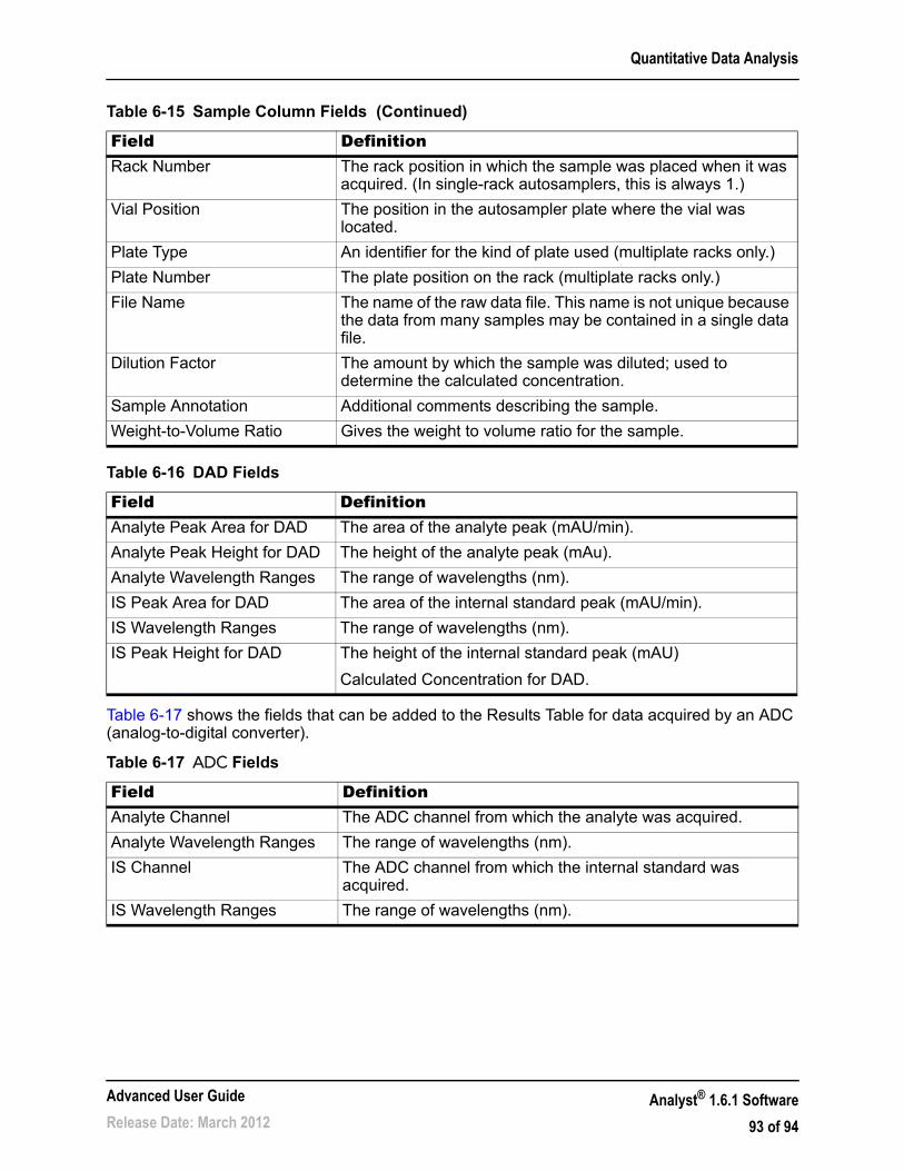
Quantitative Data Analysis
Table 6-17 shows the fields that can be added to the Results Table for data acquired by an ADC (analog-to-digital converter).
Rack Number The rack position in which the sample was placed when it was acquired. (In single-rack autosamplers, this is always 1.)
Vial Position The position in the autosampler plate where the vial was located.
Plate Type An identifier for the kind of plate used (multiplate racks only.)
Plate Number The plate position on the rack (multiplate racks only.)
File Name The name of the raw data file. This name is not unique because the data from many samples may be contained in a single data file.
Dilution Factor The amount by which the sample was diluted; used to determine the calculated concentration.
Sample Annotation Additional comments describing the sample.
Weight-to-Volume Ratio Gives the weight to volume ratio for the sample.
Table 6-16 DAD Fields
Field DefinitionAnalyte Peak Area for DAD The area of the analyte peak (mAU/min).
Analyte Peak Height for DAD The height of the analyte peak (mAu).
Analyte Wavelength Ranges The range of wavelengths (nm).
IS Peak Area for DAD The area of the internal standard peak (mAU/min).
IS Wavelength Ranges The range of wavelengths (nm).
IS Peak Height for DAD The height of the internal standard peak (mAU)
Calculated Concentration for DAD.
Table 6-17 ADC Fields
Field DefinitionAnalyte Channel The ADC channel from which the analyte was acquired.
Analyte Wavelength Ranges The range of wavelengths (nm).
IS Channel The ADC channel from which the internal standard was acquired.
IS Wavelength Ranges The range of wavelengths (nm).
Table 6-15 Sample Column Fields (Continued)
Field Definition
Advanced User Guide
Release Date: March 2012Analyst® 1.6.1 Software
93 of 94
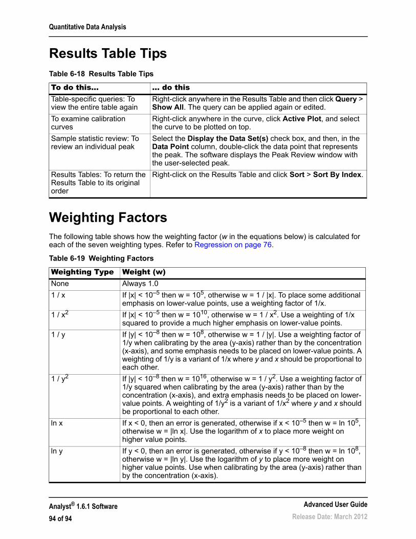
Quantitative Data Analysis
Results Table Tips
Weighting FactorsThe following table shows how the weighting factor (w in the equations below) is calculated for each of the seven weighting types. Refer to Regression on page 76.
Table 6-18 Results Table Tips
To do this... ... do thisTable-specific queries: To view the entire table again
Right-click anywhere in the Results Table and then click Query > Show All. The query can be applied again or edited.
To examine calibration curves
Right-click anywhere in the curve, click Active Plot, and select the curve to be plotted on top.
Sample statistic review: To review an individual peak
Select the Display the Data Set(s) check box, and then, in the Data Point column, double-click the data point that represents the peak. The software displays the Peak Review window with the user-selected peak.
Results Tables: To return the Results Table to its original order
Right-click on the Results Table and click Sort > Sort By Index.
Table 6-19 Weighting Factors
Weighting Type Weight (w)None Always 1.0
1 / x If |x| < 10–5 then w = 105, otherwise w = 1 / |x|. To place some additional emphasis on lower-value points, use a weighting factor of 1/x.
1 / x2 If |x| < 10–5 then w = 1010, otherwise w = 1 / x2. Use a weighting of 1/x squared to provide a much higher emphasis on lower-value points.
1 / y If |y| < 10–8 then w = 108, otherwise w = 1 / |y|. Use a weighting factor of 1/y when calibrating by the area (y-axis) rather than by the concentration (x-axis), and some emphasis needs to be placed on lower-value points. A weighting of 1/y is a variant of 1/x where y and x should be proportional to each other.
1 / y2 If |y| < 10–8 then w = 1016, otherwise w = 1 / y2. Use a weighting factor of 1/y squared when calibrating by the area (y-axis) rather than by the concentration (x-axis), and extra emphasis needs to be placed on lower-value points. A weighting of 1/y2 is a variant of 1/x2 where y and x should be proportional to each other.
ln x If x < 0, then an error is generated, otherwise if x < 10–5 then w = ln 105, otherwise w = |ln x|. Use the logarithm of x to place more weight on higher value points.
ln y If y < 0, then an error is generated, otherwise if y < 10–8 then w = ln 108, otherwise w = |ln y|. Use the logarithm of y to place more weight on higher value points. Use when calibrating by the area (y-axis) rather than by the concentration (x-axis).
Analyst® 1.6.1 Software
94 of 94
Advanced User Guide
Release Date: March 2012