advanced unit commitment strategies in the united … · risØ dtu – technical university of...

NREL is a national laboratory of the U.S. Department of Energy, Office of Energy Efficiency & Renewable Energy, operated by the Alliance for Sustainable Energy, LLC.

Contract No. DE-AC36-08GO28308

Advanced Unit Commitment Strategies in the United States Eastern Interconnection Peter Meibom and Helge V. Larsen RISØ DTU – Technical University of Denmark Roskilde, Denmark

Rüdiger Barth and Heike Brand University of Stuttgart Stuttgart, Germany

Aidan Tuohy ECAR Dublin, Ireland

Erik Ela National Renewable Energy Laboratory Golden, Colorado

Subcontract Report NREL/SR-5500-49988 August 2011

NREL is a national laboratory of the U.S. Department of Energy, Office of Energy Efficiency & Renewable Energy, operated by the Alliance for Sustainable Energy, LLC.

National Renewable Energy Laboratory 1617 Cole Boulevard Golden, Colorado 80401 303-275-3000 • www.nrel.gov

Contract No. DE-AC36-08GO28308

Advanced Unit Commitment Strategies in the United States Eastern Interconnection Peter Meibom and Helge V. Larsen RISØ DTU – Technical University of Denmark Roskilde, Denmark

Rüdiger Barth and Heike Brand University of Stuttgart Stuttgart, Germany

Aidan Tuohy ECAR Dublin, Ireland

Erik Ela National Renewable Energy Laboratory Golden, Colorado

NREL Technical Monitor: Erik Ela Prepared under Subcontract No. AFW-0-99426-01

Subcontract Report NREL/SR-5500-49988 August 2011

This publication received minimal editorial review at NREL.

NOTICE

This report was prepared as an account of work sponsored by an agency of the United States government. Neither the United States government nor any agency thereof, nor any of their employees, makes any warranty, express or implied, or assumes any legal liability or responsibility for the accuracy, completeness, or usefulness of any information, apparatus, product, or process disclosed, or represents that its use would not infringe privately owned rights. Reference herein to any specific commercial product, process, or service by trade name, trademark, manufacturer, or otherwise does not necessarily constitute or imply its endorsement, recommendation, or favoring by the United States government or any agency thereof. The views and opinions of authors expressed herein do not necessarily state or reflect those of the United States government or any agency thereof.

Available electronically at http://www.osti.gov/bridge

Available for a processing fee to U.S. Department of Energy and its contractors, in paper, from:

U.S. Department of Energy Office of Scientific and Technical Information P.O. Box 62 Oak Ridge, TN 37831-0062 phone: 865.576.8401 fax: 865.576.5728 email: mailto:[email protected]

Available for sale to the public, in paper, from:

U.S. Department of Commerce National Technical Information Service 5285 Port Royal Road Springfield, VA 22161 phone: 800.553.6847 fax: 703.605.6900 email: [email protected] online ordering: http://www.ntis.gov/help/ordermethods.aspx

Cover Photos: (left to right) PIX 16416, PIX 17423, PIX 16560, PIX 17613, PIX 17436, PIX 17721

Printed on paper containing at least 50% wastepaper, including 10% post consumer waste.

http://www.osti.gov/bridge�

mailto:[email protected]�

mailto:[email protected]�

http://www.ntis.gov/help/ordermethods.aspx�

iii

Acknowledgements The team gives great thanks to Charlton Clark and Stan Calvert of the Department of Energy for their support of this work. This work was supported under the Wind and Water Power Technologies Program under the DOE Office of Energy Efficiency and Renewable Energy. For their careful review of this document, technical review of the study, data validation, and general support, the authors wish to thank the following people: Michael Milligan, Bri-Mathias Hodge, Greg Brinkman, and Dave Corbus of NREL; Lynn Hecker and Brandon Heath of the Midwest ISO; Matt Schuerger of Energy Systems Consulting Services; Charlie Smith of UWIG; Bob Zavadil of Enernex; Jack King of RePPAE; Gary Moland and Richard Hunt of Ventyx; Alan Mullane of ECAR; and Mark O’Malley of University College Dublin. The team also would like to thank Bruce Green for his editorial support.

iv

Table of Contents 1. Introduction ........................................................................................................................................... 1 1.1. Background ................................................................................................................................... 1 1.2. Methodology Overview .............................................................................................................. 3 1.2.1. The Scenario Tree Tool .................................................................................................. 4 1.2.2. The Scheduling Model ................................................................................................... 6 1.3. Data and Data Preparation .......................................................................................................... 9 1.3.1. Measured Wind Feed in and Load Data....................................................................... 9 1.3.2. Forecast Data for Wind Speed and Load ................................................................... 10 1.3.3. Generation and Interconnection .................................................................................. 12 1.3.4. Reserve Requirements .................................................................................................. 12 2. Scenario Tree Tool Results and Analysis ....................................................................................... 14 2.1. Wind Power Forecasts .............................................................................................................. 14 2.1.1. Regional Differences .................................................................................................... 14 2.1.2. Comparison of Different Years ................................................................................... 16 2.1.3. Comparison of onshore and offshore ......................................................................... 19 2.2. Load Forecasts ........................................................................................................................... 19 2.2.1. Regional Differences .................................................................................................... 20 2.2.2. Comparison of different years ..................................................................................... 22 2.3. Forecasts of Net Load ............................................................................................................... 24 2.3.1. Regional Differences .................................................................................................... 25 2.3.2. Inter-annual comparison ............................................................................................... 26 2.4. Replacement Reserves .............................................................................................................. 29 2.5. Conclusions ................................................................................................................................ 30 3. Scheduling Model Results ................................................................................................................. 31 3.1. Costs ......................................................................................................................................... 31 3.2. Production ................................................................................................................................... 35 3.3. Reserve ........................................................................................................................................ 40 3.4. Wind Curtailment ...................................................................................................................... 49 3.5. Prices ......................................................................................................................................... 51 3.6. Interchange ................................................................................................................................. 52 3.7. Conclusions from Scheduling Model Results ........................................................................ 54 4. Coal as a Must-Run Sensitivity ........................................................................................................ 55 5. Conclusions ......................................................................................................................................... 58 5.1. Key Findings and Issues ........................................................................................................... 58 5.2. Further Work and Improvements ............................................................................................ 60 6. References ......................................................................................................................................... 62

v

List of Figures FIGURE 1: STUDY FOOTPRINT. .......................................................................................................................... 3FIGURE 2: OVERVIEW OF WILMAR PLANNING TOOL. ......................................................................................... 4FIGURE 3: CONSIDERED WIND POWER CURVES. ................................................................................................ 5FIGURE 4: ILLUSTRATION OF THE ROLLING PLANNING AND THE DECISION STRUCTURE IN EACH PLANNING PERIOD. . 8FIGURE 5: STANDARD DEVIATION OF WIND SPEED FORECAST ERROR DEPENDANT ON FORECAST HORIZON GIVEN IN

M/S. ...................................................................................................................................................... 10FIGURE 6: STANDARD DEVIATION OF LOAD FORECAST ERROR DEPENDANT ON FORECAST HORIZON GIVEN IN MW.

............................................................................................................................................................ 11FIGURE 7: STANDARD DEVIATION OF THE LOAD FORECAST ERROR IN RELATION TO THE PEAK LOAD DEPENDANT ON

FORECAST HORIZON. ............................................................................................................................. 12FIGURE 8: EXEMPLARY DAY-AHEAD FORECAST SCENARIO TREE OF THE WIND POWER FORECAST FOR THE PJM

REGION GIVEN IN MW. ........................................................................................................................... 14FIGURE 9: RELATIVE FREQUENCY OF THE RELATIVE FORECAST ERROR OF WIND POWER PRODUCTION BASED ON

THE INPUT DATA FOR THE YEAR 2004 IN ALL MARKET REGIONS. ................................................................ 15FIGURE 10: RELATIVE FREQUENCY OF THE RELATIVE FORECAST ERROR OF WIND POWER PRODUCTION BASED ON

THE INPUT DATA FOR THE YEAR 2004 IN SELECTED MARKET REGIONS. ...................................................... 16FIGURE 11: RELATIVE FREQUENCY OF THE RELATIVE FORECAST ERROR OF WIND POWER PRODUCTION FOR THE

DIFFERENT BASE YEARS IN THE NY_ISO REGION. ................................................................................... 17FIGURE 12: RELATIVE FREQUENCY OF THE RELATIVE FORECAST ERROR OF WIND POWER PRODUCTION FOR THE

DIFFERENT BASE YEARS IN THE PJM REGION. ......................................................................................... 17FIGURE 13: RELATIVE FREQUENCY OF THE RELATIVE FORECAST ERROR OF WIND POWER PRODUCTION FOR THE

DIFFERENT BASE YEARS IN THE SPP_CENTRAL REGION. ......................................................................... 18FIGURE 14: RELATIVE FREQUENCY OF THE RELATIVE FORECAST ERROR OF WIND POWER PRODUCTION FOR THE

DIFFERENT BASE YEARS IN THE TVA REGION. .......................................................................................... 18FIGURE 15: EXEMPLARY DAY-AHEAD FORECAST SCENARIO TREE OF THE LOAD FORECAST FOR THE PJM REGION

GIVEN IN MW. ....................................................................................................................................... 19FIGURE 16: RELATIVE FREQUENCY OF THE RELATIVE FORECAST ERROR OF LOAD BASED ON THE INPUT DATA OF

THE YEAR 2004 IN ALL MARKET REGIONS. ............................................................................................... 20FIGURE 17: RELATIVE FREQUENCY OF THE RELATIVE FORECAST ERROR OF LOAD BASED ON THE INPUT DATA OF

THE YEAR 2004 IN SELECTED MARKET REGIONS. ..................................................................................... 21FIGURE 18: THE FREQUENCY DISTRIBUTION OF THE RELATIVE FORECAST ERROR FOR MAPP REGION. ............... 22FIGURE 19: THE FREQUENCY DISTRIBUTION OF THE RELATIVE FORECAST ERROR FOR TVA REGION. .................. 23FIGURE 20: THE FREQUENCY DISTRIBUTION OF THE RELATIVE FORECAST ERROR FOR PJM REGION. .................. 23FIGURE 21: THE FREQUENCY DISTRIBUTION OF THE RELATIVE FORECAST ERROR FOR MISO_CENTRAL REGION.

............................................................................................................................................................ 24FIGURE 22: EXEMPLARY DAY-AHEAD FORECAST SCENARIO TREE OF NET LOAD FOR THE PJM MARKET REGION. . 25FIGURE 23: RELATIVE FREQUENCY OF THE RELATIVE FORECAST ERROR OF NET LOAD BASED ON THE INPUT DATA

OF THE YEAR 2004 IN ALL MARKET REGIONS. ........................................................................................... 26FIGURE 24: RELATIVE FREQUENCY OF THE RELATIVE FORECAST ERROR OF THE NET LOAD FOR THE DIFFERENT

BASE YEARS IN THE PJM REGION. .......................................................................................................... 27FIGURE 25: RELATIVE FREQUENCY OF THE RELATIVE FORECAST ERROR OF THE NET LOAD FOR THE DIFFERENT

BASE YEARS IN THE TVA REGION. ........................................................................................................... 27FIGURE 26: RELATIVE FREQUENCY OF THE RELATIVE FORECAST ERROR OF THE NET LOAD FOR THE DIFFERENT

BASE YEARS IN THE SPP_CENTRAL REGION. .......................................................................................... 28FIGURE 27: RELATIVE FREQUENCY OF THE RELATIVE FORECAST ERROR OF THE NET LOAD FOR THE DIFFERENT

BASE YEARS IN THE MAPP REGION. ....................................................................................................... 28FIGURE 28: AVERAGE DEMAND FOR REPLACEMENT RESERVES DEPENDANT ON THE FORECAST HORIZON FOR THE

INDIVIDUAL MARKET REGIONS FOR THE YEAR 2004 GIVEN IN MW. ............................................................ 30FIGURE 29: PRODUCTION COSTS FOR EACH YEAR. .......................................................................................... 31FIGURE 30: PRODUCTION COSTS BY UNIT COMMITMENT STRATEGY BASED ON 2006 INPUT DATA. ....................... 32FIGURE 31: PERCENT COST INCREASE OVER PERFECT FORECASTS BY UNIT COMMITMENT STRATEGY BASED ON

2006 INPUT DATA. ................................................................................................................................. 33FIGURE 32: PRODUCTION COSTS BY REGION, 2006. ........................................................................................ 34FIGURE 33: PRODUCTION BY GAS AND COAL FOR ALL YEARS. ........................................................................... 37

vi

FIGURE 34: CONTINGENCY RESERVE CARRIED ONLINE BY REGION, 2006 DATA. ................................................ 41FIGURE 35: ONLINE CONTINGENCY RESERVE BY UNIT TYPE, 2006 DATA. .......................................................... 42FIGURE 36: CONTINGENCY RESERVE CARRIED BY OFFLINE UNITS, 2006 DATA, BY REGION. ............................... 43FIGURE 37: CONTINGENCY RESERVE CARRIED OFFLINE, BY UNIT TYPE. ............................................................ 44FIGURE 38: FREQUENCY REGULATION RESERVE BY REGION, 2006 DATA. ......................................................... 45FIGURE 39: FREQUENCY REGULATION RESERVE BY UNIT TYPE, 2006 DATA. ..................................................... 46FIGURE 40: REPLACEMENT RESERVE FROM ONLINE UNITS. .............................................................................. 47FIGURE 41: ONLINE REPLACEMENT RESERVE PROVISION BY UNIT TYPE, 2006 DATA. ........................................ 48FIGURE 42: OFFLINE REPLACEMENT RESERVE PROVISION BY REGION, 2006 DATA. ........................................... 48FIGURE 43: REPLACEMENT RESERVE CARRIED BY OFFLINE UNITS, BY UNIT TYPE, 2006 DATA. ........................... 49FIGURE 44: CURTAILMENT BY YEAR. ............................................................................................................... 50FIGURE 45: CURTAILMENT BY REGION, 2006 DATA. ......................................................................................... 50FIGURE 46: INTRA-DAY PRICES, 2006 DATA. ................................................................................................... 51FIGURE 47: EXPORTS FOR REGION, 2006 DATA. ............................................................................................. 52FIGURE 48: IMPORTS BY REGION, 2006 DATA. ................................................................................................. 53FIGURE 49: NET IMPORTS BY REGION, 2006 DATA. .......................................................................................... 54FIGURE 50: PRODUCTION COSTS FOR DIFFERENT METHODS, COAL NOT MUST-RUN AND MUST-RUN RESULTS, 2006

DATA. .................................................................................................................................................... 55FIGURE 51: PRODUCTION FROM UNIT TYPE FOR COAL MUST-RUN (MR) AND NOT-MUST-RUN (NMR). ................. 56FIGURE 52: CURTAILMENT OF WIND ENERGY WITH AND WITHOUT COAL AS MUST-RUN. ....................................... 57FIGURE 53: ILLUSTRATION OF NEW LOOPING STRUCTURE ALLOWING FOR INCLUSION OF UNCERTAINTY IN THE FIRST

OPERATION HOURS IN EACH PLANNING LOOP. THE ILLUSTRATION SHOWS ROLLING PLANNING STEPPING FORWARD IN TIME IN 6-HOUR STEPS. ...................................................................................................... 60

List of Tables TABLE I: WIND CAPACITY AND ENERGY BY REGION ............................................................................................. 3TABLE II: COSTS BY YEAR AND UNIT COMMITMENT METHOD. ............................................................................. 32TABLE III: CHANGE IN PRODUCTION COSTS AS A PERCENTAGE OF PFC COSTS. ................................................. 32TABLE IV: PRODUCTION COSTS BY REGION, 2006 DATA. .................................................................................. 35TABLE V: TOTAL PRODUCTION BY FUEL TYPE, IN TWH. .................................................................................... 36TABLE VI: PRODUCTION BY FUEL TYPE, 2006 DATA, BY REGION, IN TWH. ......................................................... 38TABLE VII: PRODUCTION BY FUEL TYPE, TWH, 2006 DATA, BY REGION (CTD) ................................................... 39TABLE VIII: DATA FOR COST DIFFERENCES IN COAL MUST-RUN AND COAL NOT-MUST-RUN, 2006 DATA. .............. 56

1

1.

1.1. BACKGROUND

INTRODUCTION

During recent years, there has been tremendous growth in the amount of wind power generation in numerous countries. This growth is likely to continue. Wind power offers a non-polluting source of energy with non-volatile fuel costs. However, because of its dependence on the wind resource, it can create difficulties for utilities and system operators when managing the balance between generation and load. Wind power cannot be predicted with great accuracy and therefore system operators must plan their system with consideration of this uncertainty. This has always been true in power systems since generating resources and transmission components can fail at any time unexpectedly, and the system demand cannot be predicted with perfect accuracy. System operators will perform a unit commitment, which will determine the least cost solution of what generators need to be online to meet the expected demand. These are usually performed in advance of the operating day, and in today’s systems are generally performed one day prior to the operating day. The unit commitment performed in today’s systems is also usually deterministic in nature, and will represent uncertain (or stochastic) variables with their expected value. Operating reserve is also scheduled by the unit commitment programs to ensure the system can respond to events such as generator or transmission line outages, or demand or variable- generation forecast errors. This is carried by particular units which are withholding a portion of their capacity from providing energy (or are ramped down from their maximum output) so the system can balance supply and demand in the event of a generator or network failure or prediction error.

Advanced unit commitment methods and strategies with high penetrations of wind power have been an ongoing research topic in recent years [1] - [5]. With the uncertainty present in wind power and wind power forecasts, it is important to plan the system to be robust and efficient towards meeting multiple uncertain potential outcomes. It is also important to make best use of wind power forecasts, realizing they generally improve in accuracy as time horizons become nearer and often before ultimate decisions have to be made. This project sought to evaluate the impacts of high wind penetrations on the U.S. Eastern Interconnection and analyze how different unit commitment strategies may affect these impacts.

In January 2010, the Eastern Wind Integration and Transmission Study (EWITS) was published [6]. The study evaluated the operating impacts for 20% and 30% wind power on the majority of the Eastern Interconnection. It also evaluated different scenarios of where the wind was located as well as different transmission plans. This follow-up study was intended to further the analysis performed in EWITS by focusing on the impacts of advanced unit commitment strategies used at high penetrations of wind power. It will point to both the effect that various assumptions about modeling unit commitment will have on integration studies, as well as the effect that the strategies will have on actual system operation with high wind power. Specifically, it evaluated the use of a stochastic unit commitment and the use of rolling planning for the Eastern Interconnection. The study used consistent data with EWITS where possible. Wind power and load forecasts were built using the scenario tree tool (STT) that calculated about one thousand scenarios of the wind and load outcomes for different time horizons ahead and for each planning loop. This was reduced using sophisticated scenario reduction techniques to have a reasonable number of probabilistic forecasts with different probabilities that could be run in the stochastic scheduling model (SM). The stochastic scheduling model would minimize the expected cost of energy, but ensure that all of the reduced set of scenarios could be met reliably. The forecasts were developed to represent a new

2

update every few hours, all looking ahead up to the end of the day or end of the next day. The start-up times and other commitment constraints of units must be respected so that unit commitment must only be a binding decision if there is no more time to make an updated decision. In theory, the use of stochastic planning and frequent rolling updates to the planning and unit commitment could give great value over the traditional deterministic once-per-day unit commitment commonly performed today in the United States. By making the unit commitment to meet multiple scenarios of possible outcomes, it will more economically meet the demand on average in real-time. It ensures that costly corrections can be prevented when system conditions are far from the expected because the stochastic unit commitment also ensured those unlikely scenarios could be met reliably. Rolling planning also ensures that the unit startup is only required when the startup time, minimum run times, and minimum down times are binding and therefore, when not binding, their decision to turn on can wait until more accurate forecasts are available. This also increases the efficiency since the system startups would be based on better forecast information than if the unit commitment was restricted to day-ahead decisions only.

The objective was to use the WILMAR (Wind Power Integration in Liberalised Electricity Markets, http://www.wilmar.risoe.dk/) planning tool to evaluate each of these methods. Four model runs were used to reach this objective with the terms used in the rest of this paper in parentheses.

• Stochastic planning using scenario trees with six branches (six forecasts), unit commitment updated every 3 hours (STO).

• Stochastic planning, unit commitment for units with start times greater than 1 hour, updated once per day in the day-ahead market (UCDay)

• Deterministic planning with forecast error, and unit commitment updated every three hours (OTS). Only one wind power production and load forecast taken into account in each rolling planning period being equal to the expected wind power production and load in the scenario tree used in the stochastic model runs.

• Deterministic planning with perfect foresight (PFC) i.e. wind power and load forecasts corresponds to realized wind power and load.

The comparison of these four model runs, in terms of different operational results and costs, would give more insight into the consequences of using these unit commitment strategies with 20% wind for some or all of the eastern United States. By comparing STO with UCDay, impacts and benefits could be analyzed of rolling planning compared to keeping the unit commitment fixed in the day-ahead market. Comparing STO with OTS, the impacts and benefits could be analyzed of running the unit commitment model considering stochastic variables of wind and load with a deterministic unit commitment. The following results in this paper are derived using the EWITS scenario 2 wind placements and 2004, 2005, and 2006 wind and load time series data. Figure 1 shows the study footprint and Table I gives wind feed-in energy by region. Note that the annual energy will differ slightly from year to year due to the inter-annual variability of capacity factors.

3

Figure 1: Study footprint.

Table I: Wind capacity and energy by region

Region Onshore (MW) Offshore (MW) Total (MW) Annual Energy (TWh)

ISO-NE 8,837 5,000 13,837 46

MISO+MAPP 69,444 0 69,444 288

NYISO 13,887 2,620 16,507 48

PJM 28,192 5,000 33,192 97

SERC 1,009 4,000 5,009 16

SPP 86,666 0 86,666 245

TVA 1,247 0 1,247 4

Total 209,282 16,620 225,902 745

1.2. METHODOLOGY OVERVIEW

The WILMAR Planning Tool is used to analyze the consequences of wind power on the Eastern Interconnection. The WILMAR Planning tool consists of a number of sub-models and databases as shown in Figure 2. The green cylinders are databases, the red parallelograms indicate exchange of information between sub models or databases, the blue squares are models. The user shell controlling the execution of

4

the WILMAR Planning tool is shown in black. The main functionality of the WILMAR Planning tool is embedded in the Scenario Tree Tool (STT) and the Scheduling Model (SM).

Figure 2: Overview of WILMAR Planning tool.

1.2.1. THE SCENARIO TREE TOOL

The STT generates stochastic scenario trees containing three input parameters to the SM: wind power production forecasts, load forecasts, and demand for replacement reserves. Replacement reserves are positive reserves with activation times longer than 10 minutes and for forecast horizons from 1 hour to 36 hours ahead. The main input data for the STT is wind speed and/or wind power production data, historical electricity demand data, assumptions about wind production and load forecast accuracies for different forecast horizons and regions.

The STT consists of three modules. The first module generates a significant number of scenarios for wind power and load forecasts using the Monte-Carlo Method. Since the Scheduling Model can only handle a limited number of scenarios, a second module reduces the number of scenarios by applying a scenario reduction algorithm. The scenario reduction process will by construction remove extreme events from the reduced scenario trees. Therefore, the calculation of the replacement reserve demand by the third module enables the Scenario Tree Tool to quantify the effect that partly predictable wind power and load including the more rare extreme events has on the replacement reserve requirements for different forecast horizons.

5

Module 1

Both for load and wind power forecasts errors, Monte-Carlo simulations taking into account the individual forecast error characteristics dependant on the forecast horizon are carried out. The generation of forecast scenarios for wind power is based on a simulation of wind speed forecast errors. The simulation has to account for the error distribution which varies with increasing forecast horizons. These Monte-Carlo simulations are based on Auto Regressive Moving Average (1, 1) (ARMA (1, 1) time-series models [9]. With this approach, it is possible to account for a) autocovariances of forecast errors and b) the increase of forecast errors depending on the forecast horizon. It is assumed that the distribution of wind speed errors follows a Gaussian distribution [10]. Further, spatial correlations of wind speed forecast errors as observed in the Eastern Interconnection are explicitly taken into account [11]. To generate wind power production and load scenarios, the sample paths of wind power and load forecasts errors are added to historical time-series data of respectively wind power production and load time-series data.

The simulation of wind power forecast errors is based on wind speed time series. If only wind power time- series data are available as metered data, these power series have to be initially transformed to speed series by the use of an appropriate power curve to simulate wind speed forecast errors. In a subsequent step, the generated wind speed forecast scenarios are converted to wind power forecast scenarios. Figure 3 shows different power curves available for this study. The figure shows a Class II wind site power curve for three different area densities. More information on the use of power curves and the general methodologies of the wind speed and power data creation can be found in Brower 2010 [12].

Figure 3: Considered wind power curves.

Many sample paths of the ARMA series, that are drawn randomly, represent many different possible outcomes of forecasting. So, for example, i sample paths (or scenarios) of wind and load forecast are derived. The scenarios of wind forecasts are aggregated with the load scenarios. It is not necessary to combine every wind scenario with every load scenario and to apply the scenario reduction module to i2 scenarios in this example. It is sufficient to allocate one load scenario for each wind scenario in a random way and to apply the scenario reduction module to a large number of scenarios (e.g. i = 1000). Statistically, this leads to the same result.

0

0.3

0.6

0.9

0 5 10 15 20 25 30 35

Wind speed (m/s)

Perc

enta

ge o

f Win

d po

wer

cap

acity

class II - 1.1class II - 1.16class II - 1.18

6

Module 2

For each planning period, one thousand scenarios of forecasts are generated. Yet such a large number of forecast scenarios cannot be treated with the stochastic Scheduling Model due to computational limitations. Hence, the number of forecast scenarios is reduced by first determining the Euclidean distances between the individual forecast scenarios. One scenario of the scenario pair with the smallest Euclidean distance is deleted, and the sum of the probabilities of both scenarios is allocated to the remaining scenario. This procedure is repeated until a predefined number of scenarios is achieved. Afterwards, based on the remaining scenarios that still form a one-stage tree, a multi-stage scenario tree is constructed by deleting inner forecasts and creating branching within the scenario tree. A detailed discussion of the scenario tree reduction algorithm can be found in [13].

Module 3

The calculation of the replacement reserve demand by the Scenario Tree Tool enables the WILMAR Planning tool to quantify the effect that partly predictable load and wind power production has on the replacement reserve requirements for different forecast horizons. The demand for replacement reserve corresponds to the 90th percentile of the total forecast error of load and wind power production for all unreduced scenarios being bundled into a reduced scenario tree. It is determined by summing up the forecast error of load and wind power production among the unreduced scenarios depending on the forecasted hour and generated scenario and comparing it with the expected (average over the forecasts) load and wind in the forecasted hour. The individual demand for replacement reserves of one branch of the resulting tree thereby considers the forecast errors of all wind power and load scenarios that have been reduced to this branch.

1.2.2. THE SCHEDULING MODEL

The Scheduling Model is a stochastic, optimization model with the demand for replacement reserves, wind power production forecasts, and load forecasts as the stochastic input parameters. The model evaluates optimal unit commitment and economic dispatch at hourly time-resolution. The model minimizes the expected value of the system production costs consisting of fuel costs, start-up costs, and variable operation and maintenance costs. The expectation of the system production costs is taken over all given scenarios of the stochastic input parameters. Thereby it has to optimize the operation of the whole power system without the knowledge of which one of the scenarios will be closest to the realization of the stochastic input parameter, for example the actual wind power generation. Hence, some of the decisions, notably start-ups of power plants, have to be made before the wind power production and load (and the associated demand for replacement reserve) is known with certainty. The methodology ensures that these unit commitment and dispatch decisions are robust towards different wind power prediction errors and load prediction errors as represented by the scenario tree for wind power production and load forecasts.

The demand for positive reserves (both spinning reserves with activation times below 10 minutes and replacement reserves) determines, together with the expected values of load forecasts and wind power

7

forecasts and the technical restrictions of power plants, the day-ahead unit commitment and day-ahead power exchange between regions planned for the next 36 hours. The realized load and wind power production, together with the technical restrictions of power plants, determine the actual dispatch of the power plants and the actual power exchange in the operating hour in question. Technical restrictions of power plants are minimum and maximum stable generation levels, minimum number of operation hours and off-line hours, start-up times, piece-wise linear fuel heat rate curves and ramp-up and ramp-down rates. For the consideration of large power systems comprising a large number of power plants, it is possible to introduce into the Scheduling Model a linear approximation of the unit commitment and to aggregate similar power plants (depending on type, used fuel, and vintage) to avoid the usage of integer variables thereby saving calculation time. Because of the large number of generating units in the Eastern Interconnection (over 7,000 units in all), this approach has been used in this study. This will have the effect of not being able to examine every unit individually, and therefore, some of the benefits which may be seen in stochastic unit commitment may not be as apparent here as if a full mixed integer approach was taken. As units will be aggregated, it may not be possible to show in as fine a detail how stochastic methods will produce a better commitment of certain units.

System reserve schedules are also given as an output of the Scheduling Model. Hence, the allocation of individual types of reserves over different power plants represents one of the optimization results. The model handles contingency reserves, positive and negative frequency regulation reserves (operating on automatic generation control), and replacement reserves. The main division between categories of positive reserves is between spinning reserves that can only be provided by synchronized (i.e., on-line) units due to the short activation times of these reserves, and reserves which can be provided by both synchronized and off-line units with short start-up times (e.g., combustion turbines). In this study, half of the contingency reserve and all of the frequency regulation reserve must be spinning. For each spinning reserve category the reserve capability of a unit is restricted by a maximum reserve capability computed by 10-minute ramp-rates and the online capacity minus the generation, whichever is less. Pumped hydro storage facilities can also provide contingency reserve when in the pumping mode, because it was decided that it can respond very quickly to system needs by discontinuing pumping and therefore, decreasing the load that it had been imposing on the system.

The transmission network is represented by splitting the geographical area modelled into a number of model regions, with each model region containing a number of production and storage units and having scenario trees of load forecasts, wind power production forecasts, and demand for replacement reserves. The model regions are connected by transmission lines described by a transmission capacity and an average loss. Exchanges between regions are modelled based on a simplified transmission flow model (i.e. pipeline flow) with maximum flow between regions determined by offline studies. The grid within each modelled region is only taken into account as an average transmission and distribution loss, which in this study is part of the electricity load time-series data.

As it is not possible and realistic to cover the whole simulated time period with only a single scenario tree, the model is formulated by introducing a multi-stage recursion using rolling planning. Therewith, the unit commitment and dispatch decisions and the planned power exchanges are re-optimized taking into account that more precise wind power production and load forecasts become available as the actual operation hour gets closer in time, and taking into account the temporal technical restrictions (e.g., start-up times, minimum up and down times) of different types of power plants. The resulting production of

8

each power plant and the changes in the production and power exchange relative to the day-ahead production and power exchange plan are calculated for each hour.

In general, new information arrives on a continuous basis and provides updated information about wind power production and forecasts, the operational status of other production and storage units, and about the load. Thus, an hourly basis for updating information would be most adequate. However, stochastic optimization models quickly become intractable with increased time periods, thus, it is necessary to simplify the information arrival and decision structure in the Scheduling Model. In this study, a two-stage model is implemented. The model is able to step forward in time using rolling planning with a 3-hour step, so a one-day cycle consists of eight planning loops each modelling at hourly resolution (see Figure 4). For each time step, new simulated forecasts (i.e., a new scenario tree) that consider the change in forecast horizons are applied. This decision structure is illustrated in Figure 4, showing the scenario tree for two planning periods. For each planning period, a two-stage, stochastic optimization problem is solved having a deterministic first stage covering 3 hours, and a stochastic second stage with six scenarios covering a variable number of hours according to the rolling planning period in question. Hence, the scenario tree represents a decision structure where the system operator performs unit commitment and dispatch assuming perfect knowledge about the realized wind and load in the first three hours, and uncertain knowledge about wind and load in subsequent hours. Every three hours, there is the possibility to change the planned unit commitment and dispatch and power exchange for future hours within the limits provided by start-up times, minimum run times, and minimum down times as a response to receiving updated information about the status of the power system as the operation hours in question get closer in time. The perfect foresight assumption for the first three hours is necessary for the model, but to get a realistic unit commitment, the wind and load forecast errors within the first three hours contribute to the demand for replacement reserves in these hours.

Figure 4: Illustration of the rolling planning and the decision structure in each planning period.

12 15 18 21 00 03 0012 15 18 21 00 03 00

Rolling Planning Period 1:

Day- ahead scheduling

Rolling Planning Period 2

Stage 2Stage 1

Stage 2Stage 1

9

The rolling planning proceeds as follows; Planning loop 1 starts at 12 noon on day one and covers the 36 hours until the end of day two. The forecast horizons involved are up to 36 hours ahead. The day-ahead scheduling and power exchange is determined in Planning Period 1, as well as the realized unit commitment and dispatch, and power exchange for the first three hours in the planning loop, which happens after realization of the stochastic parameters. Furthermore, unit commitment, and dispatch, and power exchange plans are made which can cover each scenario for the individual outcome of wind power, load, and demand for replacement reserve while respecting unit commitment decisions. The probability of each scenario occurring is taken into account when considering commitment decisions.

In planning loops 2 through 8, the optimization period always ends at the end of day two, i.e., the forecast horizon of the optimization period is reduced with 3 hours in each planning loop (see Figure 4). Planning loops 5 to 8 will also start with day two, and therefore only optimize the schedules of the second day. Planning loops 2 to 8 take as a starting point the day-ahead dispatch schedules determined in planning loop 1 when rescheduling the unit commitment, dispatch, and power exchange decisions due to updated forecasts. The realized unit commitment, dispatch, and power exchange for the first three hours in each planning loop is calculated. Rescheduling plans are made for the total forecast horizon and covering each scenario of the individual outcome of the load minus wind. In planning loop 9, a new day-cycle starts now covering from 12 noon (day two) to the end of day 3.

Further detailed information about the WILMAR Planning Tool can be found in [5], [8], [14]-[16].

1.3. DATA AND DATA PREPARATION

To keep results consistent, the same data was used for this study as in the EWITS project wherever possible. However, there are key differences in the data that are important to mention. The differences are necessary because the model used is different than the simulation model used for EWITS.

1.3.1. MEASURED WIND FEED IN AND LOAD DATA

The wind data was taken from the hourly time-series data developed by AWS-Truewind for the years 2004 to 2006 [12]. Because the Scenario Tree Tool develops about one thousand scenarios for multiple forecasts of every hour of the entire year and each wind plant, it required some aggregation so that some plants were combined into larger plants. This did not negate any of the geographic diversity impacts in the data since the time series data were still added together from the modeled data. The forecast errors used as input in the STT considered the geographic diversity of the aggregated wind plants as well. The total number of “wind areas” was about 3 – 10 areas per each load region. These were separated mostly by geographic location in the region and by whether they were onshore or offshore. Once computed, this data was used as the realization of wind power in the scheduling model.

The hourly load data was gathered for use in EWITS and was also used in this study. There were 11 market regions used (Figure 1): ISO New England, NY ISO, PJM, TVA, SERC, SPP North, SPP Central, MAPP, MISO East, MISO Central, and MISO West. Each had one load time-series dataset for the three years associated with it that was used as the realization of load demand in the Scheduling Model.

10

1.3.2. FORECAST DATA FOR WIND SPEED AND LOAD

The forecast data was the key difference in input between this study and EWITS. Because probabilistic forecasts were used in the stochastic modeling, the deterministic forecasts from EWITS could not be used explicitly. Instead, the deterministic forecasts used in EWITS were analyzed so that the mean error and standard deviation were developed as a function of forecast time horizon. For wind speed, three deterministic forecasts were used in order to develop an accurate error function. These were a day-ahead forecast, a 4-hour-ahead forecast, and a 6-hour-ahead forecast. Interpolation was used to create the error calculations for all time horizons up to 36 hours ahead. The resulting standard deviation of wind speed forecast errors dependant on the forecast horizon for the individual wind areas are shown in Figure 5.

Figure 5: Standard deviation of wind speed forecast error dependant on forecast horizon given in

m/s.

For load, the day-ahead load forecast was used and representations of shorter time horizon errors were assumed based on short-term load forecast data available from various ISO websites. However, because the data for day-ahead load forecasts are produced at the same time every day, it was noticed that there was a higher dependence on the errors with the actual hour of day rather than the forecast time horizon. For instance, day-ahead load forecast statistics may show much larger errors at 20 hours ahead (forecast developed at noon day prior for 8 AM), then the errors at 36 hours ahead (forecast developed at noon day prior for midnight next day). This has much more to do with the fact that the load is more variable at 8AM then at midnight and very little to do with the forecast time horizons. For the modeling using the

0

0.5

1

1.5

2

2.5

0 2 4 6 8 10 12 14 16 18 20 22 24 26 28 30 32 34 36 Forecast hour [h]

Win

d sp

eed

[m/s

]

MISO WEST 1 MISO WEST 2 MISO WEST 3 MISO WEST 4 MISO WEST 5MAPP 1 MAPP 2 MAPP 3 ISO NE 1 ISO NE 2ISO NE 3 ISO NE 4 ISO NE 7 NY ISO 1 NY ISO 2NY ISO 3 NY ISO 4 PJM 1 PJM 2 PJM 3PJM 4 PJM 5 SERC 1 SERC 2 SPP Central 1SPP Central 2 SPP Central 4 SPP Central 5 TVA 1 TVA 2MISO Central 2 MISO Central 3 MISO Central 4 MISO East 3 MISO East 4SPP North 1 SPP North 2 SPP North 3

11

WILMAR tool, forecasts are updated every 3 hours as opposed to once per day, and so further analysis of the errors was needed for a better representation of the relationship between errors and forecast time horizon. Generally, errors should increase as forecast time horizons become greater. To alleviate this issue, the errors were smoothed out and manipulated so that the true error characteristics were still intact, but more realistic values were integrated. The resulting standard deviation of absolute load forecast errors dependant on the forecast horizon for the individual market regions are shown in Figure 6.

Figure 6: Standard deviation of load forecast error dependant on forecast horizon given in MW.

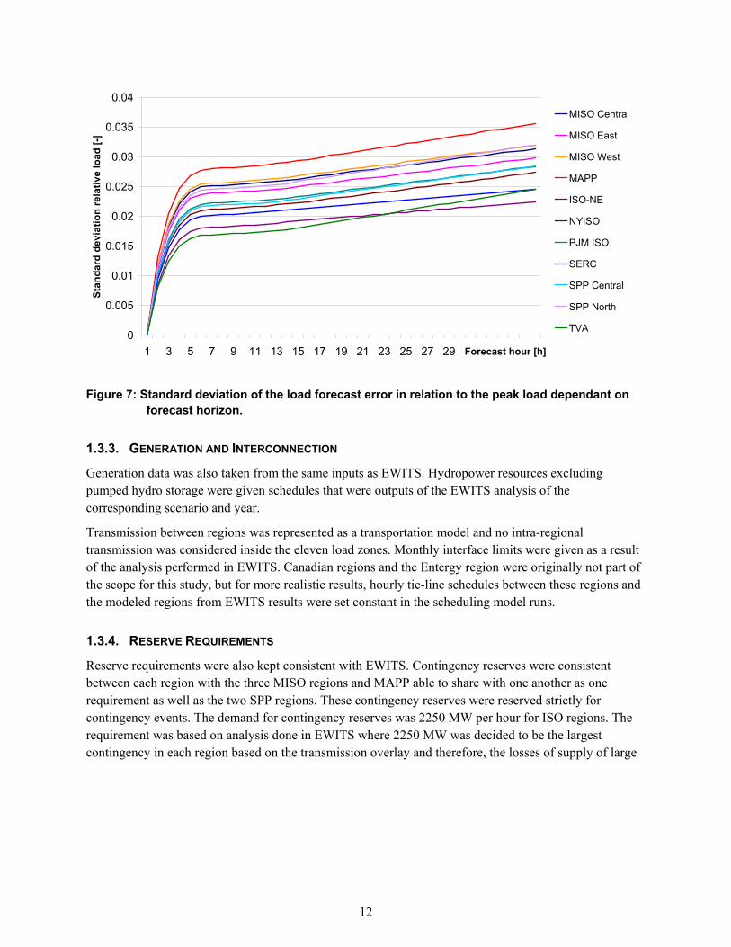
Figure 7 shows the standard deviation divided by the peak load of each market region. Whereas the absolute forecast error in the region MAPP is the lowest, the forecast error in relation to the peak load is the largest in this region. The lowest relative load forecast errors are observed in the market regions of TVA and ISO-NE.

0

1000

2000

3000

4000

5000

6000

0 2 4 6 8 10 12 14 16 18 20 22 24 26 28 30 32 34 36 Forecast hour [h]

Stan

dard

dev

iatio

n ab

solu

te lo

ad [M

W]

MISO Central

MISO East

MISO West

MAPP

ISO-NE

NYISO

PJM ISO

SERC

SPP Central

SPP North

TVA

12

Figure 7: Standard deviation of the load forecast error in relation to the peak load dependant on

forecast horizon.

1.3.3. GENERATION AND INTERCONNECTION

Generation data was also taken from the same inputs as EWITS. Hydropower resources excluding pumped hydro storage were given schedules that were outputs of the EWITS analysis of the corresponding scenario and year.

Transmission between regions was represented as a transportation model and no intra-regional transmission was considered inside the eleven load zones. Monthly interface limits were given as a result of the analysis performed in EWITS. Canadian regions and the Entergy region were originally not part of the scope for this study, but for more realistic results, hourly tie-line schedules between these regions and the modeled regions from EWITS results were set constant in the scheduling model runs.

1.3.4. RESERVE REQUIREMENTS

Reserve requirements were also kept consistent with EWITS. Contingency reserves were consistent between each region with the three MISO regions and MAPP able to share with one another as one requirement as well as the two SPP regions. These contingency reserves were reserved strictly for contingency events. The demand for contingency reserves was 2250 MW per hour for ISO regions. The requirement was based on analysis done in EWITS where 2250 MW was decided to be the largest contingency in each region based on the transmission overlay and therefore, the losses of supply of large

0

0.005

0.01

0.015

0.02

0.025

0.03

0.035

0.04

1 3 5 7 9 11 13 15 17 19 21 23 25 27 29 31 33 35 37 Forecast hour [h]

Stan

dard

dev

iatio

n re

lativ

e lo

ad [-

]

MISO Central

MISO East

MISO West

MAPP

ISO-NE

NYISO

PJM ISO

SERC

SPP Central

SPP North

TVA

13

HVDC interconnections into the region.1

[6]

The forced outage rates of generators were not a part of the stochastic input. Frequency regulation reserves for variability and within-hour uncertainty were also used with generally the same requirements as EWITS. Frequency regulation reserves are used according to the North American Electric Reliability Corporation to reduce area control error and comply with the control performance standards. Frequency regulation reserves were fulfilled per region, but with the three MISO regions able to share with one another and the same for the two SPP regions. Frequency regulation reserve would be used by units with automatic generation control to correct for area control error within the dispatch scheduling intervals. These reserve requirements can be seen in detail in . The deterministic reserve requirements in EWITS used for hourly uncertainty were ignored in this study. Instead, replacement reserves were created as a stochastic input in the STT, and were used only to cover wind and load uncertainty issues. Consequently, for the model run with perfect foresight, the demand for replacement reserves is zero.

1 This requirement was since changed in the final EWITS report due to the idea of the large HVDC connections being self-contingent. However, the requirements were kept in this study and are very close to the requirements used in the EWITS report.

14

2.

2.1. WIND POWER FORECASTS

SCENARIO TREE TOOL RESULTS AND ANALYSIS

An example of the resulting scenario trees of wind power forecasts is shown in Figure 8. It gives one set of day-ahead forecast scenarios of the wind power production for the PJM market region. Each wind power scenario has a certain probability of occurrence. Since there is no knowledge of the realized wind power and which scenario will be the closest one to the realization during the day-ahead determination of the optimal unit commitment and dispatch, the expected values of the wind power forecast shown by the blue line are taken into account. It is determined by the sum of all wind power forecast scenarios weighted with their individual probability. In subsequent loops, the forecast values are actualized. By the use of stochastic programming, the possible distribution of the forecast error is thereby represented by the set of these further forecast scenarios. Each of these scenarios has to be considered by the cost optimal unit commitment and dispatch. Whereas the deterministic treatment of forecast errors furthermore takes only into account the expected value and has no information of the possible distribution of the forecast error. Model analyses assuming forecasts with perfect foresight consider only the realized values; in this example, represented by the red line.

Figure 8: Exemplary day-ahead forecast scenario tree of the wind power forecast for the PJM region given in MW.

2.1.1. REGIONAL DIFFERENCES

The forecast errors of wind power production simulated for the different market regions and years are analyzed based on the frequency of occurrence of the forecast error relative to the installed wind power

0

5000

10000

15000

20000

25000

30000

1 3 5 7 9 11 13 15 17 19 21 23 25 27 29 31 33 35Forecast hour [h]

Win

d po

wer

pro

duct

ion

[MW

]

Scenario 1 Scenario 2 Scenario 3 Scenario 4 Scenario 5Scenario 6 Expected Value Realized Value

15

capacity. For the following analysis, only day-ahead scenario trees and the forecast horizon of 12-36 hours ahead, that is, for the following day, were considered. In addition, no distinction is made between different forecast horizons. Figure 9 shows the frequency distribution of the forecast error in all market regions based on the wind power data of 2004. This illustration is comparable to a histogram, but with interpolation between individual bins of a histogram. The distribution of the relative forecast error varies between the different regions. These differences are due to the variation of the wind speed forecast error assumed for the different areas (see section 1.3.2), and the installed capacities of the wind power stations within these areas.

Figure 9: Relative frequency of the relative forecast error of wind power production based on the

input data for the year 2004 in all market regions.

In the PJM market region, the relative wind forecast error is very small compared to regions far from the coast, like TVA and SPP_Central. In these regions, wind power forecasting leads to higher relative forecast errors. For example, in the TVA region, large relative forecast errors are observed because the forecast error standard deviation in the single wind areas ( TVA1 and TVA2) are larger than in the wind areas of the PJM region (see section 1.3.2).

For a more detailed analysis, four regions have been selected. PJM was chosen because of its high relative frequency of small relative forecast errors of the wind power production. The region TVA was chosen because it is the region with the lowest relative frequency of small relative forecast errors. Additionally, the two NY_ISO and SPP_Central regions were selected with a frequency of small forecast errors larger than in TVA, but lower than in PJM.

0

0.01

0.02

0.03

0.04

0.05

0.06

0.07

0.08

0.09

0.1

-1 -0.8 -0.6 -0.4 -0.2 0 0.2 0.4 0.6 0.8 1

Relative Forecast Error [-]

Rel

ativ

e Fr

eque

ncy

[-]

MISO_CentralMISO_East MISO_West MAPP ISO_NE NY_ISOPJM SERC SPP_Central SPP_NorthTVA

16

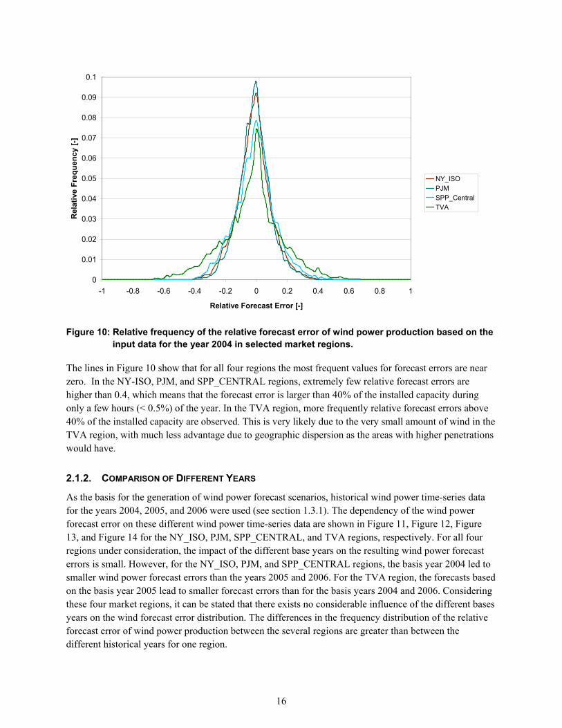
Figure 10: Relative frequency of the relative forecast error of wind power production based on the

input data for the year 2004 in selected market regions.

The lines in Figure 10 show that for all four regions the most frequent values for forecast errors are near zero. In the NY-ISO, PJM, and SPP_CENTRAL regions, extremely few relative forecast errors are higher than 0.4, which means that the forecast error is larger than 40% of the installed capacity during only a few hours (< 0.5%) of the year. In the TVA region, more frequently relative forecast errors above 40% of the installed capacity are observed. This is very likely due to the very small amount of wind in the TVA region, with much less advantage due to geographic dispersion as the areas with higher penetrations would have.

2.1.2. COMPARISON OF DIFFERENT YEARS

As the basis for the generation of wind power forecast scenarios, historical wind power time-series data for the years 2004, 2005, and 2006 were used (see section 1.3.1). The dependency of the wind power forecast error on these different wind power time-series data are shown in Figure 11, Figure 12, Figure 13, and Figure 14 for the NY_ISO, PJM, SPP_CENTRAL, and TVA regions, respectively. For all four regions under consideration, the impact of the different base years on the resulting wind power forecast errors is small. However, for the NY_ISO, PJM, and SPP_CENTRAL regions, the basis year 2004 led to smaller wind power forecast errors than the years 2005 and 2006. For the TVA region, the forecasts based on the basis year 2005 lead to smaller forecast errors than for the basis years 2004 and 2006. Considering these four market regions, it can be stated that there exists no considerable influence of the different bases years on the wind forecast error distribution. The differences in the frequency distribution of the relative forecast error of wind power production between the several regions are greater than between the different historical years for one region.

0

0.01

0.02

0.03

0.04

0.05

0.06

0.07

0.08

0.09

0.1

-1 -0.8 -0.6 -0.4 -0.2 0 0.2 0.4 0.6 0.8 1


Rel

ativ

e Fr

eque

ncy

[-]

NY_ISOPJM SPP_Central TVA

17

Figure 11: Relative frequency of the relative forecast error of wind power production for the

different base years in the NY_ISO region.


different base years in the PJM region.

0

0.01

0.02

0.03

0.04

0.05

0.06

0.07

0.08

0.09

0.1

-1 -0.8 -0.6 -0.4 -0.2 0 0.2 0.4 0.6 0.8 1


Rel

ativ

e Fr

eque

ncy

[-]

NY_ISO 2004NY_ISO 2005NY_ISO 2006

0

0.01

0.02

0.03

0.04

0.05

0.06

0.07

0.08

0.09

0.1

-1 -0.8 -0.6 -0.4 -0.2 0 0.2 0.4 0.6 0.8 1


Rel

ativ

e Fr

eque

ncy

[-]

PJM 2004PJM 2005PJM 2006

18


different base years in the SPP_Central region.


different base years in the TVA region.

0

0.01

0.02

0.03

0.04

0.05

0.06

0.07

0.08

0.09

0.1

-1 -0.8 -0.6 -0.4 -0.2 0 0.2 0.4 0.6 0.8 1


Rel

ativ

e Fr

eque

ncy

[-]

SPP_Central 2004SPP_Central 2005SPP_Central 2006

0

0.01

0.02

0.03

0.04

0.05

0.06

0.07

0.08

0.09

0.1

-1 -0.8 -0.6 -0.4 -0.2 0 0.2 0.4 0.6 0.8 1


Rel

ativ

e Fr

eque

ncy

[-]

TVA 2004TVA 2005TVA 2006

19

2.1.3. COMPARISON OF ONSHORE AND OFFSHORE

In section 1.3, we explain that the forecast error of wind speed in wind areas with offshore wind power stations (e.g. ISO-NE 7, NY-ISO 4, PJM 5 and SERC 2) is larger than of onshore wind areas. One might think that in regions with offshore wind power stations the total wind power forecast error is larger, yet this is not the case. In regions with offshore wind, the wind speed forecast error of onshore areas is comparably low (see 1.3.2). As the majority of the wind power capacity is installed in onshore areas, these regions have lower total wind power forecast errors than regions in the Midwest. For future scenarios with an increasing number of offshore wind parks, it is likely that the total wind power forecast error will become larger for these regions.

2.2. LOAD FORECASTS

An example of the resulting day-ahead scenario tree for load in the PJM region is shown in Figure 15. The forecast scenarios for load show very small differences compared to the forecast scenarios for wind power (see section 2.1). As the relative forecast error for load is very small, the expected value is very similar to the realized value.

Figure 15: Exemplary day-ahead forecast scenario tree of the load forecast for the PJM region

given in MW.

0

20000

40000

60000

80000

100000

120000

1 3 5 7 9 11 13 15 17 19 21 23 25 27 29 31 33 35Forecast hour [h]

Load

[MW

]

Scenario 1 Scenario 2 Scenario 3 Scenario 4 Scenario 5Scenario 6 Expected Value Realized Value

20


Comparable to wind, the analysis of forecast errors of load in a certain region is based on the frequency of occurrence of the forecast errors relative to the peak load in this region. For the analyses, only the values of the day-ahead trees were considered with a forecast period of 12-36 hours ahead. Again, no distinction is made between different forecast horizons. The frequency distribution of the relative forecast errors of load is shown in Figure 16. Due to the assumption of a Gaussian distribution of the load forecast error, positive forecast errors occur nearly as often as negative forecast errors. If a region has a lower standard deviation of load forecast errors (see section 1.3.2 ), the corresponding frequency distribution shows more forecast errors near to zero. In the TVA and ISO_NE regions , the frequency of small forecast errors is comparably high whereas the MAPP region has the lowest frequency of small forecast errors. In general, large forecast errors occur very infrequently in comparison to wind (see section 2.1.1).

Figure 16: Relative frequency of the relative forecast error of load based on the input data of the

year 2004 in all market regions.

Figure 17 shows the frequency distribution of the relative forecast error of load based on the input data of the year 2004 in the MAPP, PJM, TVA, and MISO_CENTRAL regions. The MAPP region was selected because it has the highest frequency of large forecast errors. TVA was selected because it is the region with the best load forecast. Additionally the MISO_Central and PJM regions have been chosen as representative of regions where the quality of the load forecast is ranked in between. For all regions the relative load forecast error lies during 99.95 % of the hours within the 10% interval.

0

0.05

0.1

0.15

0.2

0.25

0.3

0.35

-1 -0.8 -0.6 -0.4 -0.2 0 0.2 0.4 0.6 0.8 1


Rel

ativ

e Fr

eque

ncy

[-]

MISO_CentralMISO_EastMISO_WestMAPPISO_NENY_ISOPJMSERCSPP_CentralSPP_NorthTVA

21

Figure 17: Relative frequency of the relative forecast error of load based on the input data of the year 2004 in

selected market regions.

0

0.05

0.1

0.15

0.2

0.25

0.3

0.35

-1 -0.8 -0.6 -0.4 -0.2 0 0.2 0.4 0.6 0.8 1


Rel

ativ

e Fr

eque

ncy

[-]

MAPPPJMTVAMISO_Central

22

2.2.2. COMPARISON OF DIFFERENT YEARS

Similar to the analyses of the influence of the different base years 2004, 2005, and 2006 on the wind power forecast error, the impact of the load time-series data of these years on the load forecast error is shown in the following four figures.

Figure 18: The frequency distribution of the relative forecast error for MAPP region.

0

0.05

0.1

0.15

0.2

0.25

0.3

0.35

-1 -0.8 -0.6 -0.4 -0.2 0 0.2 0.4 0.6 0.8 1


Rel

ativ

e Fr

eque

ncy

[-]

R_MAPPR_MAPPR_MAPP

23

Figure 19: The frequency distribution of the relative forecast error for TVA region.

Figure 20: The frequency distribution of the relative forecast error for PJM region.

0

0.05

0.1

0.15

0.2

0.25

0.3

0.35

-1 -0.8 -0.6 -0.4 -0.2 0 0.2 0.4 0.6 0.8 1


Rel

ativ

e Fr

eque

ncy

[-]

TVA 2004TVA 2005TVA 2006

0

0.05

0.1

0.15

0.2

0.25

0.3

0.35

-1 -0.8 -0.6 -0.4 -0.2 0 0.2 0.4 0.6 0.8 1


Rel

ativ

e Fr

eque

ncy

[-]

PJM 2004PJM 2005PJM 2006

24

Figure 21: The frequency distribution of the relative forecast error for MISO_CENTRAL region.

Similar to the wind forecast error, the selection of the base year has only a negligible influence on the frequency of the load forecast error as shown here for the TVA, PJM and MISO_CENTRAL market regions. Significant differences are only depicted for the MAPP region. There, the base year 2005 leads to the smallest relative deviations, whereas the base year 2006 displays the largest relative deviations. These differences can be traced back to the fact that the peak load, the reference taken for the analyses of the load forecast error, varies between the base years. In the MAPP region, the peak load deviates between the base years up to 30 % in comparison to the base year 2004. Whereas in the TVA, PJM and MISO_Central market regions analyzed here, the differences in peak load are very small.

2.3. FORECASTS OF NET LOAD

An example of scenario trees of net load (load minus wind power feed-in) is shown in Figure 22. It considers those scenario trees of wind power and load forecasts in the PJM market region that are shown in section 2.1 and 2.2. In this example, primarily during the forecast horizon between 20 and 33 hours ahead, the expected values are underestimating the realized net load. In the subsequent planning loops, the electricity generation of the conventional power plants has to be adapted so that the finally realized net load is covered in a minimal cost optimization.

0

0.05

0.1

0.15

0.2

0.25

0.3

0.35

-1 -0.8 -0.6 -0.4 -0.2 0 0.2 0.4 0.6 0.8 1


Rel

ativ

e Fr

eque

ncy

[-]

MISO_Central 2004MISO_Central 2005MISO_Central 2006

25

Figure 22: Exemplary day-ahead forecast scenario tree of net load for the PJM market region.


Analyzing the frequency distribution of the forecast error of the net load, the time-series data of the realized net load in each region were determined. For the calculation of the frequency of occurrence of the forecast error, the difference between the realized net load and the expected forecast of the net load was divided by the maximum of the realized net load of the considered year. Figure 23 shows the frequency distribution of the error of net load for all considered regions. In the MAPP and SPP_CENTRAL regions, more frequently the forecast error is high and reaches more often values above 0.2. For regions like TVA and SERC, in more than 90 % of the hours the relative forecast error lies in the interval [-0.2, 0.2]. In regions with a low percentage of wind power production compared to its large load, like PJM and SERC, the frequency distribution of the net load forecast error is similar to the frequency distribution of the forecast error of load. In regions with a dominant share of wind power production, like MAPP, SPP_CENTRAL and SPP_North, the influence of the forecast error of wind power production on the frequency distribution of the net load forecast error is obvious.

0

20000

40000

60000

80000

100000

120000

1 3 5 7 9 11 13 15 17 19 21 23 25 27 29 31 33 35Forecast hour [h]

Net

Loa

d [M

W]

Scenario 1 Scenario 2 Scenario 3 Scenario 4 Scenario 5Scenario 6 Expected Value Realised Value

26

Figure 23: Relative frequency of the relative forecast error of net load based on the input data of the year 2004 in all market regions.

2.3.2. INTER-ANNUAL COMPARISON

The choice of the base year has only a negligible influence on the frequency distribution of the forecast error of net load in the PJM, TVA and SPP_CENTRAL regions (see Figure 24, Figure 25 and Figure 26). Only in the MAPP market region, the difference in the frequency distribution of the forecast error of net load between the different base years is larger than in the other regions (see Figure 27). This can be explained with the strong varying peak load of these regions between the different base years (see section 2.2.2).

0

0.05

0.1

0.15

0.2

0.25

0.3

0.35

-1 -0.8 -0.6 -0.4 -0.2 0 0.2 0.4 0.6 0.8 1


Rel

ativ

e Fr

eque

ncy

[-]

MISO_CentralMISO_EastMISO_WestMAPPISO_NENY_ISOPJMSERCSPP_CentralSPP_NorthTVA

27

Figure 24: Relative frequency of the relative forecast error of the net load for the different base

years in the PJM region.


years in the TVA region.

0

0.05

0.1

0.15

0.2

0.25

0.3

0.35

-1 -0.8 -0.6 -0.4 -0.2 0 0.2 0.4 0.6 0.8 1


Rel

ativ

e Fr

eque

ncy

[-]

PJM 2004PJM 2005PJM 2006

0

0.05

0.1

0.15

0.2

0.25

0.3

0.35

-1 -0.8 -0.6 -0.4 -0.2 0 0.2 0.4 0.6 0.8 1


Rel

ativ

e Fr

eque

ncy

[-]

TVA 2004TVA 2005 TVA 2006

28


years in the SPP_Central region.


years in the MAPP region.

0

0.05

0.1

0.15

0.2

0.25

0.3

0.35

-1 -0.8 -0.6 -0.4 -0.2 0 0.2 0.4 0.6 0.8 1


Rel

ativ

e Fr

eque

ncy

[-]

SPP_Central 2004SPP_Central 2005SPP_Central 2006

0

0.05

0.1

0.15

0.2

0.25

0.3

0.35

-1 -0.8 -0.6 -0.4 -0.2 0 0.2 0.4 0.6 0.8 1


Rel

ativ

e Fr

eque

ncy

[-]

MAPP 2004MAPP 2005MAPP 2006

29

2.4. REPLACEMENT RESERVES

With replacement reserves, a supplementary reserve category for the coverage of forecast errors of wind power feed-in and load is introduced (see section 1.3.4). Comparable to the treatment of forecast errors, replacement reserves are considered only in the model runs with an imperfect representation of forecasts. For stochastic model runs, the scenario trees contain individual demand values in the several scenario branches corresponding to the individual load and wind power forecast error described. With deterministic model runs, one value of the demand for replacement reserves dependant on the forecast horizon according to the expected value of load and wind power forecast is considered. Since no forecast error of load and wind power is described by the model runs with perfect foresight, no demand for replacement reserves is considered for these model runs.

The resulting average demand for replacement reserves dependant on the forecast horizon for the individual market regions is depicted in Figure 28 based on the year 2004. In general, the demand for replacement reserves increases with advancing forecast horizon. One can see the influence of the assumed increase of the standard deviation of load and wind speed forecast errors on the extent of the demand for replacement reserves (see Figure 5 and Figure 6). Furthermore, the level of replacement reserves is dependent on the wind power feed-in and the load in the considered market region. Those market regions with the largest wind power capacity installed, like SPP_Central, SPP_North, MISO_West, and PJM, show the largest demand for replacement reserves. The comparable high demand for replacement reserves in the SERC market region can be explained with the high load level and corresponding larger forecast errors of load. Consequently, the MAPP and MISO East market regions with low installed wind power capacities and low load show the smallest demand for replacement reserves. Because the forecast errors for load and wind power production by trend do not show large differences between the historical base years considered (see sections 2.1 and 2.2), the choice of the historical base year has no significant influence on the demand for replacement reserves.

30

Figure 28: Average demand for replacement reserves dependant on the forecast horizon for the

individual market regions for the year 2004 given in MW.

2.5. CONCLUSIONS

With the existing methodologies applied by the STT, the stochastic input parameters ( i.e., scenario trees of forecast errors of load and wind production as well as the demand for replacement reserves) that are required by the Scheduling Model have been generated. The data on standard deviation of wind forecast errors depending on the forecast horizon could be considered and represented well. Yet data available on load forecast errors were more detailed than for previous studies and show a distinct dependency not only on the forecast horizon but further on the forecasted hour of the day. For example, the given load forecast errors are typically higher during the morning and evening hours than during night. Hence, the algorithm to simulate load forecasts has to be extended to consider the dependency on the hour of the day. However, the dependence of the standard deviation of the load forecast error on the forecasted hour as assumed for this study could be represented well.

0

1000

2000

3000

4000

5000

6000

7000

8000

1 3 5 7 9 11 13 15 17 19 21 23 25 27 29 31 33 35 Forecast hour [h]

Rep

lace

men

t res

erve

s [M

W]

ISO_NEMAPPMISO_CentralMISO_EastMISO_WestNY_ISOPJMSERCSPP_CentralSPP_NorthTVA

31

3. Using the data described in the previous sections, the scheduling model was run for 3 different years, using EWITS scenario 2 wind placements and 2004, 2005, and 2006 wind and load time-series data. The model is implemented in GAMS and solved using the CPLEX solver

SCHEDULING MODEL RESULTS

[17]. A stochastic model run using a scenario tree with 6 branches and 3-hourly rolling planning takes approximately 160 hours to run on a personal computer with an Intel Core i5 CPU – 650 with 3.2 GHz and 3.9 GB of RAM. A deterministic model run takes approximately 35 hours on the same computer.

The remainder of this section examines the most relevant results seen from the scheduling model for this study. For some of the important results, such as costs, all three years are examined so that a comparison of different years as well as different scheduling strategies can be seen. For other results, one year is picked as an illustrative year, as results for all 3 years are similar. The model reports hourly results, showing dispatches, costs, emissions, interchanges etc. for all regions. Here, the totals or averages are given to examine the overall impact; however, it should be noted that these results are based on actual expected operation, and would include results for high wind/ low load days, low wind/ high load days (i.e., the full range of operation that would be seen when operating a system with this amount of wind power).

3.1. COSTS

The first result to examine in this study is the total production costs. As the objective of the model is to minimize production costs, this will give a good indication of the differences between unit commitment strategies. Production costs here are based on fuel usage, including startup costs. Figure 29 shows production costs for the four different unit commitment strategies for each of the three years. Table II and Table III show the results and the percent increase in costs over the perfect forecast scenario, respectively.

Figure 29: Production costs for each year.

55000

56000

57000

58000

59000

60000

61000

62000

63000

64000

2004 2005 2006

Prod

ucti

on C

osts

(M$)

OTS

PFC

STO

UCDay

32

Table II: Costs by year and unit commitment method.

Year OTS (M$) PFC (M$) STO (M$) UCDay (M$) 2004 61,526.1 61,253.6 61,537.9 61,795.9 2005 62,422.5 62,075.3 62,437.1 62,715.6 2006 58,688.1 58,055.4 58,564.5 59,259.2

Table III: Change in production costs as a percentage of PFC costs.

Year OTS STO UCDay 2004 0.44% 0.46% 0.89% 2005 0.56% 0.58% 1.03% 2006 1.09% 0.88% 2.07%

The highest costs occur from keeping unit commitment fixed from the day ahead. The two cases where rolling commitment is employed every three hours with imperfect forecasts have very similar costs in all years but 2006. In 2006, the case that uses stochastic scheduling produces 0.2% less costs. Figure 30 and Figure 31 show the production costs and increase in costs compared to the hypothetical perfect forecast case for each unit commitment strategy for the year 2006.

Figure 30: Production costs by unit commitment strategy based on 2006 input data.

57,400

57,600

57,800

58,000

58,200

58,400

58,600

58,800

59,000

59,200

59,400

OTS PFC STO UCDay

Prod

ucti

on C

osts

s (M

$)

33

Figure 31: Percent cost increase over perfect forecasts by unit commitment strategy based on

2006 input data.

For 2006, the most expensive strategy, UCDay, increases costs 2.1% compared to the perfect forecast case. The next most expensive, OTS, increases the costs about 1.1%. Finally, the STO case increases the costs from the perfect forecast case about 0.9%. This shows that with imperfect forecasts, the lowest production costs come from performing unit commitment towards multiple scenarios and updating the unit commitment more frequently. The use of rolling planning, updating the unit commitment every three hours compared to once a day, gave higher cost savings compared to using stochastic unit commitment. With imperfect forecasts, the savings of rolling planning for the Eastern Interconnect amount to about $778 million (STO minus UCDay), while the savings from using stochastic unit commitment compared to deterministic amount to about $206 million (STO minus OTS). For the other two years, the savings of using rolling planning are about half, and a savings from using stochastic unit commitment are not apparent. These years may have been over-committing more often with the stochastic case and therefore, not gathering the benefits of planning toward multiple scenarios. 2006 also had significantly more wind power than the other two years.

By updating unit commitment every three hours, efficient start and stop decisions could be made when forecasts are improved. When updating the unit commitment once a day, as is done in most systems today, system operators are stuck with the decisions they made while forecasts may have been less accurate, even if physically they would be able to change the decision. This could lead to inefficient over-commitment when net demand becomes lower than it was forecast, or under-commitment when net demand becomes higher than it was forecast. Under-commitment would lead to the use of more expensive fast-start units or use of operating reserves. Stochastic unit commitment strategies prepare the system for a series of potential outcomes. In theory, the unit commitment will have more resources online to meet the lower net demand scenarios. However, when real-time outcomes end up occurring further from the median (deterministic forecast), the stochastic solution will be better prepared to meet the real-time outcome more efficiently.

0.00%

0.50%

1.00%

1.50%

2.00%

2.50%

OTS STO UCDay

34

To examine in more detail the differences in costs between unit commitment strategies, each region was examined separately for one year. Figure 32 shows these results.

Figure 32: Production costs by region, 2006.

It can be seen that the UCDay case is generally more expensive in most of the regions. PJM and MISO_Central had the largest increases in the UCDay case compared to the other cases due to increased production in coal generation when it could not be shut down when not needed, and gas generation when coal generation could not be turned on when needed. TVA had cheaper costs from the UCDay case showing the inefficient use of the transmission system, especially since two of the largest interfaces with TVA with this transmission system are PJM and MISO Central. As expected, the PFC case is slightly less expensive than the other three cases in most of the regions. Table IV shows these results in more detail.

0

2,000

4,000

6,000

8,000

10,000

12,000

14,000

16,000

18,000

R_IS

O_N

E

R_M

APP

R_M

ISO

_Cen

tral

R_M

ISO

_Eas

t

R_M

ISO

_Wes

t

R_N

Y_IS

O

R_PJ

M

R_SE

RC

R_SP

P_Ce

ntra

l

R_SP

P_N

orth

R_TV

A

Prod

ucti

on C

osts

(M

$)

UCDay

STO

OTS

PFC

35

Table IV: Production costs by region, 2006 data.

Region OTS (M$) (M$) PFC (M$) (M$) STOC (M$) UCDay (M$)

R_ISO_NE 2,014 1,936 1,988 2,061

R_MAPP 1,343 1,343 1,335 1,311

R_MISO_Central 7,019 7,000 6,997 7,297

R_MISO_East 3,771 3,773 3,763 3,748

R_MISO_West 4,522 4,542 4,518 4,616

R_NY_ISO 2,307 2,179 2,249 2,282

R_PJM 15,077 15,091 15,047 15,304

R_SERC 8,300 8,142 8,242 8,207

R_SPP_Central 3,095 3,012 3,195 3,373

R_SPP_North 3,253 3,043 3,173 3,207

R_TVA 7,987 7,995 7,974 7,853

Total 58,688 58,056 58,481 59,259

3.2. PRODUCTION

The next result examined is the difference in production by fuel type for different unit commitment strategies. Table V shows that there is a difference in production from year to year for the different cases; as wind production increases (highest is 2006; lowest is 2004) due to a higher capacity factor, coal power decreases. Nuclear and hydro are mostly coming in as fixed schedules and therefore, do not change much between the three years. Wind produces 19% of all energy in 2004, about 19.7% in 2005, and between 20.5-20.7% in 2006.

36

Table V: Total production by fuel type, in TWh.

One of the most significant impacts on production costs is the difference between natural gas and coal production. Figure 33 shows the coal and gas production for each case and each year. For all three years, UCDAY has the highest gas production. UCDAY is not able to commit coal during forecast errors that require additional supply in real-time. Gas units, however, have fast start times and are mostly used to accommodate these forecast errors. The other differences are not as obvious. STO has slightly higher coal production in most years. During many days and hours, STO may be committing additional resources for uncertainty, and when that uncertainty does not occur, it may have overcommitted the coal, requiring it to potentially curtail wind power.

OTS PFC STO UCDAY

2004 2005 2006 2004 2005 2006 2004 2005 2006 2004 2005 2006 Coal 1,698 1,681 1,630 1,697 1,680 1,629 1,699 1,683 1,633 1,698 1,682 1,637 Gas 29 38 36 29 37 34 29 38 35 39 39 37 Uranium 887 886 885 887 886 886 887 886 885 887 886 889 Hydro 143 143 144 143 143 144 143 143 144 143 143 144 Wind 658 680 706 656 678 709 653 676 705 653 676 704 Pumped Hydro 17 19 17 17 19 16 17 19 17 17 19 18 Total 3,432 3,447 3,418 3,429 3,443 3,418 3,428 3,445 3,419 3,437 3,445 3,429

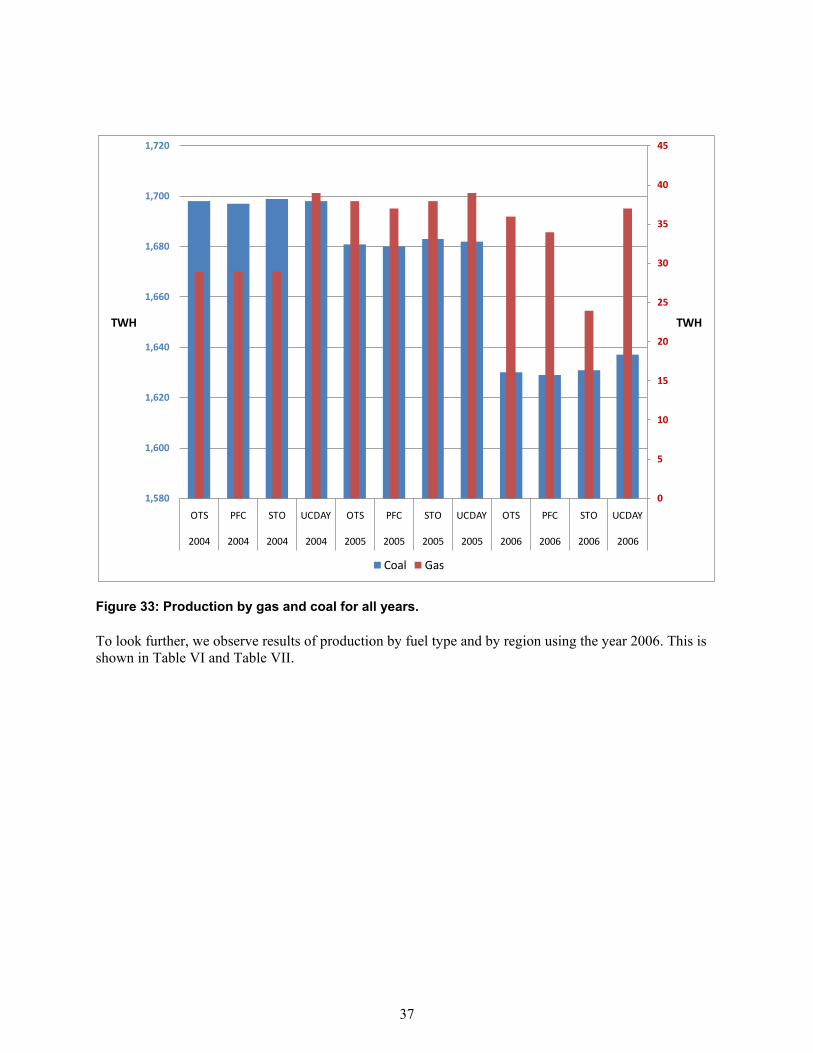
37

Figure 33: Production by gas and coal for all years.

To look further, we observe results of production by fuel type and by region using the year 2006. This is shown in Table VI and Table VII.

0

5

10

15

20

25

30

35

40

45

1,580

1,600

1,620

1,640

1,660

1,680

1,700

1,720

OTS PFC STO UCDAY OTS PFC STO UCDAY OTS PFC STO UCDAY

2004 2004 2004 2004 2005 2005 2005 2005 2006 2006 2006 2006

TWHTWH

Coal Gas

38

Table VI: Production by fuel type, 2006 data, by region, in TWh.

Type Fuel R_ISO_NE R_MAPP R_MISO_Central R_MISO_East R_MISO_West

OTS

Coal 17.2 67.3 241.2 120.7 170.2

Electricity 5.2 1.4

Gas 5.0 0.4 0.5 0.0 1.7

Uranium 48.6 43.1 49.5 34.4

Water 21.7 7.4 1.6 0.5 2.7

Wind 46.4 42.2 35.9 18.8 138.0

Total 144.1 117.3 322.3 190.9 347.0

PFC

Coal 16.9 67.3 241.7 120.9 172.0

Electricity 5.3 1.3

Gas 4.6 0.4 0.3 1.7

Uranium 48.6 43.1 49.5 34.4

Water 21.7 7.4 1.6 0.5 2.7

Wind 46.4 42.2 35.9 18.8 138.0

Total 143.5 117.3 322.6 191.0 348.8

STO

Coal 17.2 67.3 241.3 120.6 170.9

Electricity 5.2 1.3

Gas 4.8 0.4 0.4 0.0 1.7

Uranium 48.6 43.1 49.5 34.4

Water 21.7 7.4 1.6 0.5 2.7

Wind 46.4 42.2 35.9 18.8 138.0

Total 144.0 117.3 322.3 190.7 347.6

UCDAY

Coal 19.1 71.4 245.6 119.6 171.5

Electricity 4.7 1.1

Gas 4.6 0.6 1.2 0.0 2.0

Uranium 48.5 3.9 43.1 49.5 34.3

Water 21.7 7.4 1.6 0.5 2.7

Wind 46.4 42.2 35.9 18.8 137.8

Total 145.0 125.5 327.5 189.5 348.4

39

Table VII: Production by fuel type, TWh, 2006 data, by region (ctd).

Type Fuel R_NY_ISO R_PJM R_SERC R_SPP_Central R_SPP_North R_TVA OTS Coal 389.5 195.2 80.2 66.0 255.5 389.5

Electricity 2.1 1.8 1.4 0.2 0.9 2.1

Gas 2.7 3.2 7.7 8.6 1.3 2.7

Uranium 314.6 227.8 16.5 92.7 314.6

Water 7.3 12.1 5.0 0.5 18.2 7.3

Wind 102.9 15.3 126.4 123.8 4.3 102.9

Total 819.2 456.3 220.7 215.7 372.9 819.2

PFC Coal 26.0 390.5 192.4 79.7 65.6 256.0

Electricity 3.5 2.1 1.8 1.5 0.2 0.8

Gas 4.2 2.7 2.9 7.6 7.8 1.3

Uranium 58.4 314.6 227.8 16.5 92.7

Water 66.6 7.3 12.1 5.0 0.5 18.2

Wind 52.5 102.9 15.3 128.6 124.4 4.3

Total 211.1 820.2 453.2 222.3 215.1 373.3

STO Coal 26.7 389.7 195.8 81.7 66.1 255.5

Electricity 3.5 2.1 2.0 1.5 0.2 0.9

Gas 4.4 2.6 2.8 8.1 8.4 1.3

Uranium 58.4 314.6 227.8 16.5 92.7

Water 66.6 7.3 12.1 5.0 0.5 18.2

Wind 52.5 102.9 15.3 125.5 123.0 4.3

Total 212.2 819.3 456.7 221.7 214.7 372.9

UCDAY Coal 24.8 393.2 192.8 81.6 66.4 250.8

Electricity 3.5 2.6 3.8 1.5 0.2 0.9

Gas 4.8 3.1 2.6 9.0 8.4 1.2

Uranium 58.4 314.6 227.8 16.5 92.7

Water 66.6 7.3 12.1 5.0 0.5 18.2

Wind 52.5 102.9 15.3 126.1 122.2 4.3

Total 210.6 823.7 455.2 223.1 214.3 368.0

Since there is a great deal of trading between regions, and the model is optimizing over the entire system and not individually between regions, there does not seem to be one region which best exemplifies what

40

happens in general. However, certain regions seem to show some interesting results. For example, NY_ISO shows a decrease in coal usage for UCDay, and a lower total production overall; as can be seen by the increased total costs for UCDay, this would imply that this region makes less than optimal exchanges to other regions in the UCDay case. Here, inflexible coal may be utilized less to prevent wind curtailment either in NY_ISO or elsewhere.

3.3. RESERVE

This study required multiple types of reserve, some of which are more effected by increased wind power than others, as described in 1.3.4. Here, the data for 2006 is taken as an illustrative example of what occurs in each year – upon examination, each year shows approximately similar relative results for reserve, so only one year is examined.

Figure 34 shows the contingency reserve carried online by region for each method in 2006. The requirement for contingency reserve as discussed in section 1.3.4, is 2250 MW for all regions with 50% (1125 MW) required to be online (spinning). The spinning requirement can also be seen in Figure 34. The sum of MISO East, MISO West, MISO Central and MAPP and the sum of SPP Central and SPP North should therefore be greater than the requirement of the contingency reserve region (shown as A_SPP and A_MISO in Figure 34). It can be seen that approximately the same amount is carried in most regions. In some regions, like in NYISO and SPP, the amount of contingency reserves online is equal to or just barely above the requirement, meaning that there are some costs in requiring the contingency reserves during some hours. In other regions, like TVA and SERC, the average amount of contingency reserves online is substantially higher than the requirement for the STO and OTS cases. This is because some solutions allow additional reserve to be carried as units are already online to manage uncertainty. It could also be when there are not enough offline reserve and more have to be online to meet the total contingency reserve requirement. However, the next section shows this is not the case. This is due to the constraint being modeled as an inequality; in certain hours some solutions will already have enough units online to more than cover a particular contingency. In these hours the marginal costs of providing spinning reserve from online units (contingency reserve and positive frequency regulation reserve) are zero, because enough units are kept online irrespective of the demand for spinning reserve. Lastly, it is seen that MAPP, with the smallest capacity of all regions that contribute to the MISO contingency reserves actually holds the majority of the online contingency reserves.

41

Figure 34: Contingency reserve carried online by region, 2006 data.

Figure 35 shows the contingency reserve carried by online units, distributed by unit type. Overall it appears that OTS carries the most contingency reserve online. This is due to the fact that the hydro units are not being used to meet other stochastic scenarios and are therefore available online to supply contingency reserves. This should be the same for PFC, since it also does not need to meet multiple scenarios. We see that for the PFC the pumped hydro provides majority and so these are interchangeably used for providing the contingency reserve online.

0

200

400

600

800

1000

1200

1400

1600A

_ISO

_NE

A_M

APP

A_M

ISO

_Cen

tral

A_M

ISO

_Eas

t

A_M

ISO

_Wes

t

A_M

ISO

A_N

YISO

A_P

JM

A_S

ERC

A_S

PP_C

entr

al

A_S

PP_N

orth

A_S

PP

A_T

VA

MW

UCDay

STO

OTS

PFC

Requirement

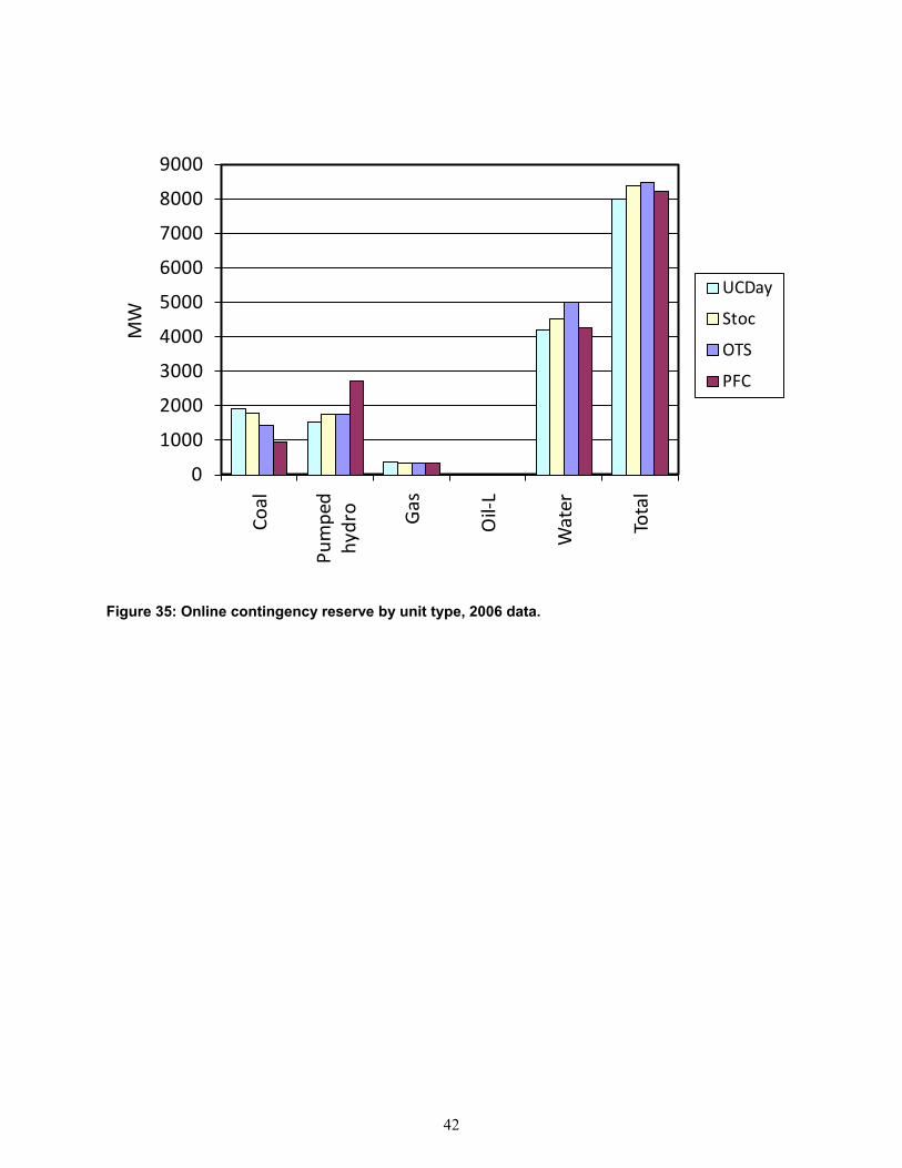
42

Figure 35: Online contingency reserve by unit type, 2006 data.

0

1000

2000

3000

4000

5000

6000

7000

8000

9000

Coal

Pum

ped

hydr

o Gas

Oil-

L

Wat

er

Tota

l

MW

UCDay

Stoc

OTS

PFC

43

The same year and data is shown for contingency reserve carried by offline units, as shown in Figure 36 and Figure 37.

Figure 36: Contingency reserve carried by offline units, 2006 data, by region.

0

5000

10000

15000

20000

25000

30000

35000

40000

45000

A_I

SO_N

E

A_M

APP

A_M

ISO

_Cen

tral

A_M

ISO

_Eas

t

A_M

ISO

_Wes

t

A_M

ISO

A_N

YISO

A_P

JM

A_S

ERC

A_S

PP_C

entr

al

A_S

PP_N

orth

A_S

PP

A_T

VA

Cont

inge

ncy

Rese

rve

Off

line

(MW

)

UCDay

STO

OTS

PFC

44

Figure 37: Contingency reserve carried offline, by unit type.

It can be seen that most regions carry more contingency reserve offline when wind production is known perfectly. The demand for replacement reserves is zero when wind and load is known perfectly and hence, no offline units are required to provide replacement reserves in this case, making more units available for contingency reserves. The operational costs of providing offline reserves are in most cases zero, because these gas and oil-fired units would have been kept offline irrespective of the demand for offline reserves, due to their high marginal costs. The contingency reserve being carried offline is slightly higher for the UCDay case, particularly for gas units as shown in Figure 37. PJM and SERC regions also have over 40,000 MW and 30,000 MW of combustion turbines in their systems, respectively, and therefore, the sum of offline contingency reserve and offline replacement reserve is very close to the total sum of their capacities, since their actual production is usually small. Two other important concepts should be mentioned. First, the results are for all times of year including spring time, where wind power is very high, load is low, and these resources will be offline regardless. Second, the model never simulates the high resolution needs of actual contingencies that require the contingency reserve, and therefore, it does not show how these resources would actually be used in the simulation, only how they are held ready to be used.

0

20000

40000

60000

80000

100000

120000

140000

Gas

Oil-

L

MW

UCDay

Stoc

OTS

PFC

45

The next category of reserve, frequency regulation reserve, is again examined by region and unit type. Frequency regulation reserve is required in both the positive and negative directions. Figure 38 shows the distribution by region as well as the average requirement.

Figure 38: Frequency regulation Reserve by region, 2006 data.

For frequency regulation reserve, MISO_Central, MISO_East, and MISO_West all contribute to MISO regulating reserve, and SPP_Central and SPP_North contribute to SPP regulating reserve. PFC can be seen to carry more frequency regulation reserve in most regions. Some of the regions, like NYISO, do not schedule more than the requirement. The marginal cost of positive frequency regulation reserve for this region was greater than zero every hour and was as high as $200/MWh, and the marginal cost of negative frequency regulation reserve was often greater than zero as well. On the other hand, TVA and SERC had more than enough frequency regulation reserve for most hours. In practice, regulation reserve has additional costs due to additional wear and tear that is caused which would likely keep the amounts closer to the requirements. Shown by unit type in Figure 39, you can see that the main changes between unit commitment strategies are in the hydro plants. As discussed for the online contingency reserve, the PFC case is like the OTS case, and does not model hydro units based on meeting additional scenarios and therefore, there are more hydro units with large ramp rates that are able to provide more frequency regulation reserve than needed. Hydro units have large ramp rates and for these reserves, are mostly only constrained to provide reserves by their maximum capacities. Conventional units are dispatched differently for the different unit commitment methods; they would be operating at different levels above their minimum generation level and below their maximum generation level giving the difference of amounts.

0

1,000

2,000

3,000

4,000

5,000

6,000

UCDay

STO

OTS

PFC

Requirement

46

Figure 39: Frequency regulation reserve by unit type, 2006 data.

The next category of reserve, replacement reserve, is required to cover for longer term variation from wind and load forecast. It is not needed in the PFC case; therefore, only the 3 methods that contain uncertainty in the wind and load forecasts are given here (STO, UCDay, and OTS). Figure 40 shows a clear difference between those different methods of unit commitment and comparison with the replacement reserve demand. All of the figures for replacement reserve would show the quantities of replacement reserve provision for the first stage, or real time (i.e., first three hours of the planning loop).

0

5,000

10,000

15,000

20,000

25,000

Coal Pumped Hydro Gas Hydro Total

UCDay

Stoc

OTS

PFC

47

Figure 40: Replacement reserve from online units.

It can be seen that UCDay carries more online replacement reserve in general, as it needed to keep more units online to deal with the increased uncertainty seen in the unit commitment when it is only carried out once a day. STO carries more reserve in general than OTS, as it is modeling the uncertainty explicitly.

Figure 41 shows online replacement reserve by unit type. Storage is used for replacement reserve only very rarely since it will be supplying contingency reserve and frequency regulation reserve for most of the time. The largest contributor to online replacement reserve is coal units. This is because coal units have relatively smaller ramp rates and therefore, may still have additional capacity available, but which is ramp-constrained from providing contingency reserve or frequency regulation reserve. Since replacement reserve is set aside for potential needs many hours ahead, ramp rates would not be binding.

0

200

400

600

800

1000

1200

1400

1600A

_ISO

_NE

A_M

APP

A_M

ISO

_Cen

tral

A_M

ISO

_Eas

t

A_M

ISO

_Wes

t

A_N

YISO

A_P

JM

A_S

ERC

A_S

PP_C

entr

al

A_S

PP_N

orth

A_T

VA

MW

UCDay

Stoc

OTS

48

Figure 41: Online Replacement reserve provision by unit type, 2006 data.

Figure 42: Offline replacement reserve provision by region, 2006 data.

0

500

1000

1500

2000

2500

3000

3500

4000

4500

5000

Coal

Pum

ped

Hydr

o Gas

Hydr

o

Tota

l

UCDay

Stoc

OTS

0

2000

4000

6000

8000

10000

12000

14000

16000

A_I

SO_N

E

A_M

APP

A_M

ISO

_Cen

tral

A_M

ISO

_Eas

t

A_M

ISO

_Wes

t

A_N

YISO

A_P

JM

A_S

ERC

A_S

PP_C

entr

al

A_S

PP_N

orth

A_T

VA

MW UCDay

Stoc

OTS

49

Replacement reserve can be carried by offline units more in the STO case. This means that units do not need to be online and costing money, but still providing reserve. As seen in Figure 43, this is carried mostly by gas combustion turbines with some contribution from oil combustion turbines, both quick starting units.

Figure 43: Replacement reserve carried by offline units, by unit type, 2006 data.

3.4. WIND CURTAILMENT

Wind curtailment is generally a significant impact when examining integration. Here, the four different methods are examined to show how much curtailment is affected by method of operation for each year. Figure 44 shows the curtailment for each solution, sorted by method and year. You can see that the least amount of curtailment occurs during the perfect forecast case (5-7% reduction in wind curtailment from STO to PFC, with higher reduction in 2006 compared to 2004 and 2005). The perfect forecast case will schedule as much wind power as possible ahead of time and does not run into the issue of under-forecasting. When wind power is under-forecast, it is more likely that transmission congestion or minimum generation limits will be reached. Total curtailment is approximately 54 TWh to 70 TWh, depending on year and method; this is approximately 8.5% (2004) to greater than 10% (2006) of total production from wind, as shown in the production section. You can also see that stochastic cases (STO and UCDay) have the most curtailment. Even though stochastic scheduling is better for optimizing over all scenarios, there is more likelihood of over-committing than there is in the deterministic cases.

0

10000

20000

30000

40000

50000

60000G

as

Oil-

L

Tota

l

MW

UCDay

Stoc

OTS

50

Figure 44: Curtailment by year.

Figure 45 shows that most of the curtailment happens in the SPP regions, where there is a large amount of wind with respect to its amount of interchange. Curtailment is mostly inevitable with all unit commitment strategies if insufficient transmission or flexibility is built to accommodate the heavy amount of wind in this region. However, the advanced unit commitment strategies provide a modest decrease in the amount of curtailment, only slightly higher than the PFC case.

Figure 45: Curtailment by region, 2006 data.

50

55

60

65

70

75

2004 2005 2006

Curt

ailm

ent (

TWh)

OTS

PFC

STO

UCDay

0.00

5.00

10.00

15.00

20.00

25.00

30.00

35.00

40.00

45.00

50.00

R_IS

O_N

E

R_M

APP

R_M

ISO

_Cen

tral

R_M

ISO

_Eas

t

R_M

ISO

_Wes

t

R_NY

_ISO

R_PJ

M

R_SE

RC

R_SP

P_Ce

ntra

l

R_SP

P_No

rth

R_TV

A

TWh

UCDay STO OTS PFC

51

3.5. PRICES

While WILMAR does not seek to emulate markets, the marginal cost of balancing load and demand in each time period gives an indication of what prices may be like. WILMAR produces prices for all time periods and planning loops through the marginal cost of the load balance equation for each region, which for stochastic periods will be calculated from the expected value of the marginal cost. Day-ahead and real-time prices and everything in between can be calculated. The prices between look-ahead periods and the real-time should converge to being equal in a market setting and since the study is not emulating market behavior, we show only the intra-day prices from the first three hours to explain how the marginal cost of energy may differ for the four cases. This is shown in Figure 46.

In general, the differences in prices can come from times when natural gas is the marginal provider and when coal is the marginal provider. Intra-Day prices can be seen to be the highest with the OTS case, followed by UCDay. OTS is not minimizing the expected cost over multiple potential scenarios, which may lead to under-commitment scenarios where combustion turbines may need to be turned on in real-time. UCDay may often commit too little capacity as well since updated forecasts cannot be used to turn on slow-start units. In the day ahead, combustion turbines can be planned for differently for each scenario and therefore, for the unlikely scenarios the UCDay case is relying on waiting to turn the combustion turbines on in real time, where the combustion turbines have high marginal costs. PFC is the lowest price, with STO slightly higher. STO has low marginal costs as this mode keeps more units online to manage the uncertainty in many potential outcomes, thereby reducing marginal cost as it won’t need to use as much of the combustion turbines in real time. For PFC, it is because its unit commitment solution is always the most efficient, and combustion turbines will never be needed due to forecast errors.

Figure 46: Intra-day prices, 2006 data.

0

10

20

30

40

50

60

R_IS

O_N

E

R_M

APP

R_M

ISO

_Cen

tral

R_M

ISO

_Eas

t

R_M

ISO

_Wes

t

R_NY

_ISO

R_PJ

M

R_SE

RC

R_SP

P_Ce

ntra

l

R_SP

P_No

rth

R_TV

A

Intr

a Day

Pric

e ($

/M

Wh)

UCDay STO OTS PFC

52

3.6. INTERCHANGE

Interchange is scheduled in the model between regions using Net Transfer Capability; therefore, the interchanges are scheduled so that those areas with lower costs will export, and higher costs will import up to the maximum capability of the interface.

Exports from each region for 2006 are shown in Figure 47:

Figure 47: Exports for region, 2006 data.

There is very little difference in most cases. The STO and OTS cases seem to have similar exports in most regions. However, some regions export more – for example, PJM . MISO East shows a decrease in exports, as seen with a decrease in production.

0

20,000,000

40,000,000

60,000,000

80,000,000

100,000,000

120,000,000

Expo

rts

(MW

h)

UCDay

STO

OTS

PFC

53

Figure 48: Imports by region, 2006 data.

You can see from Figure 48 that most imports occur into the PJM and SERC regions. Again, UCDay sees the biggest difference in imports, indicating that exchanges are less optimally scheduled with this method compared to others, and thus cause an increase in costs. For example, SERC imports more; this may indicate that it needs to import to make up for forecast errors.

Figure 49 shows the net imports for each region for 2006 data. Only one region changes from net imports to net exports based on this modeling method, and that is a very slight change in the MISO Central area. There are small differences between the intra-day (UCDAY) and day-ahead methods (OTS, PFC and STO) however, particularly in SERC, PJM, NYISO, and MISO Central and East. For example, net imports are increased in NYISO, and decreased in PJM, both of which are net importers. This would imply that operation of the interchanges is one of the reasons for the differences in costs seen for day- ahead only commitment.

0

50,000,000

100,000,000

150,000,000

200,000,000

250,000,000Im

port

s (M

Wh)

UCDay

STO

OTS

PFC

54

Figure 49: Net imports by region, 2006 data.

3.7. CONCLUSIONS FROM SCHEDULING MODEL RESULTS

Overall, this section compared two different types of results. Firstly, there was a comparison from year to year. This would show how dependent on a particular year certain results were. It could be seen that different wind and load time-series data did produce different results, and different years could increase or decrease production costs and other results for all methods. 2006 had the most wind power feed-in production and the lowest load, leading to it having the lowest production costs. It also had the most significant production cost differences between the advanced unit commitment techniques. In 2004 and 2005, the stochastic scheduling did not seem to have any benefit in terms of production cost over deterministic unit commitment. Compared to 2006, stochastic scheduling did not use as little gas as deterministic scheduling did. The deterministic scheduling strategy did not have as many times where it had to start gas units in 2004 and 2005 due to under-forecasting, as it did in 2006, relative to stochastic scheduling, where forecast errors are better modeled in advance.

Other results included the overall power production, wind curtailment, energy prices, reserve provision, and interconnection. The main difference in power production was between the gas, coal, and wind power. The way the system scheduled these three fuel types is what determined the overall cost for the most part. However, the interchange between regions could affect the results as well. Different regions have different costs for each of the fuels and inefficiencies in scheduling could cause sub-optimal interchange schedules. The prices found from each of the methods showed higher prices with OTS and UCDay for the year shown. These methods had gas on the margin more often setting these prices. The wind curtailment was highest for methods applying the stochastic scheduling strategy. This is because these methods will often over-commit due to the possibility of under-forecasting, often causing more need to curtail the wind power.

-150,000,000

-100,000,000

-50,000,000

0

50,000,000

100,000,000

150,000,000

200,000,000

250,000,000N

et Im

port

s (M

Wh)

UCDay

STO

OTS

PFC

55

4. The purpose of this report is to provide more analytical information on the impact that changing methods of unit commitment will have on the results for variable generation integration studies, and the implications that it could have for system operation. In EWITS, coal was assumed to be ‘must-run,’ and it was decided to run a sensitivity analysis in this study with this constraint as well. Therefore, the same model was run with one year of data (2006) where the only constraint was that all coal units had to be online (unless forced out) and running above their minimum generation limits. The previous results examined in this report (section

COAL AS A MUST-RUN SENSITIVITY

3) were for coal that could be cycled, that is, the system operator can commit and de-commit coal with long minimum run and minimum down times, and slow ramp rates to reflect coal’s relative lack of flexibility. By operating coal in this mode, its use should be better optimized. This section compares the results for the 2006 coal case (i.e. must-run) and that shown in section 3 (with coal not-must-run for the year 2006).

Here, only those results that are significantly affected by the change are examined. Other results did not change significantly, and are therefore not shown here.

There is a significant difference in total production costs, as shown in Figure 50.

Figure 50: Production costs for different methods, coal not must-run and must-run results, 2006

data.

It can be seen that relaxing the must-run constraint on coal reduces costs, as expected. By removing this constraint, coal can be turned off or ramped down if this is the best option for overall system cost.

Table VIII shows the data so that percentage changes can be examined. You can see that model run STO is more expensive than OTS, PFC, and UCDay when coal is treated as must-run, that is, the advantage of using stochastic rolling planning dissapeares in this case. The cost advantage of allowing coal to decommit from time to time is between 3% and 4.5% of system costs corresponding to $1.776 billion to

56500

57000

57500

58000

58500

59000

59500

60000

60500

61000

61500

OTS (M$) PFC (M$) STO (M$) UCDay (M$)

Prod

ucti

on c

ost

(M$)

Coal must run Coal not must run

56

$2.629 billion, a significant amount of money. The cost advantage is biggest for the most advanced UC strategy (STO) and lowest for the one without intra-day rescheduling (UCDay).

Table VIII: Data for cost differences in coal must-run and coal not-must-run, 2006 data.

OTS (M$)

PFC (M$) STO (M$)

UCDay (M$)

Coal Must-Run 60803 60457 61111 61035

Coal Not Must-Run 58688 58055 58481 59259

Coal Must-Run - increase vs. STO -0.5% -1.1% 0.0% -0.1%

Coal Not-Must-Run - increase vs. STO 0.4% -0.7% 0.0% 1.3%

Increase with coal must-run -3.6% -4.1% -4.5% -3.0%

Another area of interest for the comparison of coal must-run versus not-must-run is production by unit type. Figure 51 shows the comparison for those units that produce more than 1 TWh. Firstly, you can see that the method does not have a great impact on the changes from must-run to not-must-run. You can see that coal is increased, as expected when coal is must-run and production from gas and wind power is decreased. The high minimum generation levels of the coal units lead to more curtailment of wind generation (between 4 and 8 TWh, depending on the UC strategy) in the coal as must-run case.

Figure 51: Production from unit type for coal must-run (MR) and not-must-run (NMR).

0

200

400

600

800

1,000

1,200

1,400

1,600

1,800

Prod

ucti

on (T

Wh) STO NMR

STO MR

UCDay NMR

UCDay MR

PFC NMR

PFC MR

OTS NMR

OTS MR

57

The impact on wind curtailment is further shown in Figure 52. Wind curtailment increases between 5% (STO) and 12% (PFC) when coal is must-run. The reduction of wind curtailment is a major advantage of moving to flexible options to cycle coal on and off. The pattern of wind curtailment depending on UC method is the same for coal must-run and not-must-run, with the lowest wind curtailment in PFC and highest in UCDay.

Figure 52: Curtailment of wind energy with and without coal as must-run.

0

10

20

30

40

50

60

70

80

90

OTS PFC STO UCDay

Curt

ailm

ent (

TWh)

Coal must run Coal not must run

58

5.

5.1. KEY FINDINGS AND ISSUES

CONCLUSIONS

This study set out to provide more analysis on the effect of assumptions about unit commitment methods on integration studies such as the Eastern Wind Integration and Transmission Study. Taking that study’s inputs as a starting point, it modeled the Eastern Interconnection (without transmission overlays, but with exchange limits between regions) with 2004, 2005, and 2006 wind and load time-series data using the WILMAR planning tool. The purpose of this report is not to run sensitivities on the EWITS report, because it uses different assumptions about units (they are aggregated here) and transmission (this model only examines transfers between regions as opposed to a DC or full AC power flow). Instead, it was to examine the different unit commitment methods and how they may impact operation of the system with high wind, as well as how the assumptions about unit commitment affect results in these types of integration studies.

The model is divided into two main sections; the STT, which provides scenarios of wind and load using forecast data, and the scheduling model, which runs production cost modeling, using the scenarios from the STT to optimize the unit commitment stochastically. Three years were examined to gauge the impact that particular data pertaining to individual years would have.

From the STT results, the following were the key findings:

• It could be seen that certain regions produced better wind forecasts than others; all regions had the vast majority of their forecasts under 40% error.

• Demand forecasting could be seen to perform better in certain hours and certain look-ahead horizons; this is different than other studies where the error was assumed constant, and will need to be examined.

• For net load forecasts, certain regions performed better than others in forecasting the demand net of wind. The error in net load was consistent throughout the years for the majority of regions.

• Replacements reserve demand was different for each region and with increasing time horizon.

The scenario trees produced were then used for the scheduling model. The following are the key findings from the results of the scheduling model:

• Costs are more significantly affected by the presence of rolling planning (i.e., re-planning the system every 3 hours) than by treating stochastic variables stochastically or deterministically; planning unit commitment once a day results in an increase in production costs of approximately 1-2%, whereas deterministic schedules only had higher costs from the stochastic scheduling case for one of the three years. However, we note that a comparison between stochastic and deterministic scheduling between two methods where unit commitment was once a day may show different results and we encourage this analysis in the future. Stochastic UC may produce more significant cost savings on a day-ahead only unit commitment.

• Perfect foresight reduced the costs compared to stochastic with rolling planning with 0.5-1%. The reduction is caused by the significant reduction in wind curtailment in the perfect foresight case.

59

• Results across all three years, while varying from year to year (i.e., 2006 data with higher wind capacity factors was less costly and showed greater benefits of both rolling planning and stochastic scheduling) do not show significant differences in terms of the difference between methods, which is the main focus of this study. However, the 2006 data showed much more significant benefits of using both stochastic unit commitment and rolling planning. The other years may have had more occurrence of over-commitment when planning for more robust operation. In other words, there were more occurrences of the system ready for an increase in net load, but the net load did not increase as often. Tweaking of the operating reserves and the cost of not having enough reserve could potentially bring the results closer to the operator preference (as opposed to being too risk averse).

• Gas units had to be used more in the deterministic and non rolling cases to adjust for forecast errors in wind power production and electricity demand, while coal units could be better used in the other schedules since the more efficient solution methods chose them due to their lower cost.

• Wind curtailment was 5-7% lower in the perfect foresight case compared to the stochastic scheduling with rolling planning due to no over-committing of units taking place in the perfect foresight case. In general, wind curtailment was very high, consisting of 8.5% to over 10% of total possible wind power production, dependant on year. The high wind curtailment was located in SPP_Central and SPP_North, indicating that these regions will need to increase transmission capacities to neighboring regions if they are going to accommodate the planned amounts of wind power.

• Prices derived from marginal unit costs were affected by choice of method; Intra-Day prices was seen to be the highest, with the OTS case followed by UCDay. OTS is not minimizing the expected cost over multiple potential scenarios, which may lead to under-commitment scenarios where combustion turbines may need to be turned on in real time. UCDay may often commit too little capacity as well since updated forecasts cannot be used to turn on slow-start units. PFC achieves the lowest price, with STO slightly higher. STO has low marginal costs as this mode keeps more units online to manage the uncertainty in many potential outcomes, thereby reducing marginal cost as it won’t need to use as much of the combustion turbines in real time. For PFC, it is due to the fact that its unit commitment solution is always the most efficient and combustion turbines will never be needed due to forecast errors.

• Transmission between regions was also affected by the type of unit commitment; the results for day-ahead commitment only used the transmission less optimally, resulting in more units being online than needed in some regions, with the opposite in other regions. The deterministic solutions tended to use transmission more, with higher net imports for net importers and higher exports for net exporters.

• If coal was assumed must-run, as in EWITS, there was shown to be an increase in costs of 3% to 4.5%. Coal could not be shut off at times of high wind; it has to remain online. This means there is less room to turn down generation to avoid wind curtailment. The subsequent increase in wind curtailment means wind energy, with no fuel cost, is wasted, increasing overall costs. Gas production is reduced when coal is must-run; therefore, more flexible gas is being replaced by coal, which means balancing of wind and load is only possible with curtailment. This is consistent with the view that gas is well suited to balancing wind, due to its greater ramping rates and lower minimum generation levels.

60

• When coal is must-run, the cost benefits of moving to stochastic rolling planning are not as clear as when it can be committed and de-committed by the model because there is limited flexibility to change the unit commitment schedules intra-day due to the coal units being must-run.

5.2. FURTHER WORK AND IMPROVEMENTS

Future research should focus on introducing uncertainty into the first 3 hours of each planning period. This could be done by changing the WILMAR model into alternating between stochastic model runs with uncertainty in all future operation hours, calculating the unit commitment of slow units, and deterministic model runs using the realised values of wind power production and load to calculate the final dispatch of the slow units and the unit commitment and dispatch of the fast units (see Figure 53). In the stochastic model runs, the unit commitment of the slow units would need to be restricted to be the same across scenarios within the start-up time of the unit. Such model development is already in progress at Risø DTU.

Figure 53: Illustration of new looping structure allowing for inclusion of uncertainty in the first

operation hours in each planning loop. The illustration shows rolling planning stepping forward in time in 6-hour steps.

The comparison of the different unit commitment strategies took careful attention in modeling and contrasting. The scenario of unit commitment fixed in the day-ahead timeframe and modeled deterministically however, was never compared with the other cases. This model scenario is the most closely related to today’s operation. If this case was compared with others, some of the results may have differed. For example, if this case was compared with UCDay, the benefits of stochastic unit commitment may have been better seen. We also believe that the continuous linear relaxation of the unit status variable had an impact on the results. Smaller test systems and improvements in solution techniques could allow

1812 18 24 06 12 24

Stochastic Day-ahead scheduling

Stage 1 (now)

Realised values – only possible to change unit commitment of fast units

Intra-day rescheduling

Realised values


Realised values


Realised values

61

the use of integer variables. System operators today are using integer programming in their unit commitment programs either through lagrangian relaxation or branch-and-bound MIP techniques, and therefore, would be implementing any advancement to their unit commitment programs with the same usage of integers. We are convinced that the usage of integers would show the benefits of stochastic rolling planning more clearly. For example, the All Island Grid Study (Ireland), which used integers due to the much smaller system, found benefits of stochastic unit commitment of 0.9% [5]. Other constraints, for example, the detailed modeling of combined cycle plants, could also have shown a difference in results. The more constraints that the system operator will implement in their unit commitment program, the more difficult it becomes to plan deterministically with higher uncertain variable resources, and the more difficult it becomes to plan once per day given the use of less accurate forecasts. This theory should be tested in future studies. Lastly, we would like to discuss the actual implementation of these strategies. Many ISOs in the United States have already implemented hour-ahead or shorter unit commitment updates, mostly for the commitment of combustion turbines. These models have short optimization horizons (e.g., less than 3 hours) and less decision variables. Improvements in solution techniques can allow for longer optimization horizons as are discussed in this report, and for the start-up of any unit that has ample time to start-up according to its start-up times. It should be noted that many of these generating facilities may have staffing requirements, and that this type of requirements should be built into their start-up cost and start-up time requirements. We believe that stochastic unit commitment techniques, though not seen with significant value in this study, can improve the cost efficiency and reliability of power system operations. Most ISOs require a deadline within which their markets must be closed. Therefore, solution techniques would have to improve the computation time required to solve these large problems in sufficient time. More research should be performed to determine the optimal scenario set. For example, three scenarios; a low, medium, and high, may be the sufficient number that can be solved in a reasonable time. Finally, the use of probabilistic forecasts has received little attention in most of these studies. In stochastic unit commitment studies including this one, a forecast is created based on the statistics of a large set of data from the stochastic variable. For example, a year’s worth of data for one wind plant was used to create the standard deviation for various forecast horizons, and this was used to make a probabilistic forecast based on a normal distribution of wind speed. In reality, these probabilistic forecasts are commonly created by organizations that specialize in wind forecasting using a combination of meteorological and statistical information. Meteorological inputs may show different probability density functions for different times based on the meteorological phenomena. This may impact how the stochastic unit commitment programs benefit system reliability. We encourage research on using meteorological-based probabilistic forecasts to understand more of these questions.

62

6. [1] L. Wu, M. Shahidehpour, T. Li, “Stochastic security-constrained unit commitment,” IEEE

Transactions on Power Systems, vol. 22, no. 2, pp. 800-811, May 2007.

REFERENCES

[2] François Bouffard et al, “Security for operations planning with significant wind power generation,” IEEE Transactions on Power Systems, vol. 23, no. 2, pp. 306-316, May 2008.

[3] T. Yong, R. Entriken, P. Zhang, “Reserve determination for system with large wind generation,” Proceedings of Power & Energy Society General Meeting, Calgary, Canada, July 2009.

[4] J. Morales, A. Conejo, J. Perez-Ruiz, “Economic valuation of reserves in power systems with high penetration of wind power,” IEEE Transactions on Power Systems, vol. 24, no. 2, pp. 900-910, May 2009.

[5] A. Tuohy, P. Meibom, M. O’Malley, “Unit commitment for systems with significant wind penetration,” IEEE Transactions on Power Systems, vol. 24, no.2, pp. 592-601, May 2009.

[6] North American Electric Reliability Corporation, BAL-001 and BAL-005, “Reliability Standards for the Bulk Electric Systems of North America,” June 2010.

[7] Enernex Corporation, “Eastern Wind Integration and Transmission Study,” Prepared for the National Renewable Energy Laboratory, January 2010.

[8] P. Meibom, R. Barth, B. Hasche, H. Brand, M. O’Malley, “Stochastic optimization model to study the operational impacts of high wind penetrations in Ireland”, IEEE Transactions on Power Systems, vol. 26, no. 3, pp. 1367-1379, August 2011.

[9] W. H. Greene, Econometric analysis. Pearson Education. Upper Saddle River, 2003 [10] M. Lange and U. Focken, Physical approach to short-term wind power prediction. Springer.

Berlin, 2006. [11] L. Söder, “Simulation of wind speed forecast errors for operation planning of multi-area power

systems,“ in Proc. 8th International Conference on Probabilistic Methods Applied to Power Systems, Ames, 2004.

[12] Michael Brower, “Development of Eastern Regional Wind Resource and Wind Plant Output Datasets,” NREL-SR\550-46764, December 2009.

[13] J. Dupacova, N. Gröwe-Kuska, and W. Römisch, “Scenario reduction in stochastic programming - an approach using probability metrics”, Math. Program., Ser. A 95, vol. 3, pp. 493-511, 2003.

[14] Barth R., Brand H., Meibom P., and Weber C. A stochastic unit commitment model for the evaluation of the impacts of the integration of large amounts of wind power. Proc. 9th International Conference on Probabilistic Methods Applied to Power Systems, Stockholm, Sweden 2006.

[15] Meibom P., Barth R., Brand H., Swider D. J., Ravn H., and Weber C., All Island Grid Study workstream 2B - wind variability management studies, Department of Enterprise, Trade and Investment, 2008.

[16] Wind power integration in liberalised electricity markets (WILMAR) project. Available: http://www.wilmar.risoe.dk.

[17] GAMS: The Solver Manuals, version 23.3, Washington, DC: GAMS, 2005.

http://www.wilmar.risoe.dk/�

advanced unit commitment strategies in the united … · risØ dtu – technical university of...

Documents