Advanced Undergraduate LaboratoryExperiment 10, FTS

Fourier Transform Spectroscopy

December 25, 2013

1

1 Introduction: The Wiener-Khinchin Theorem

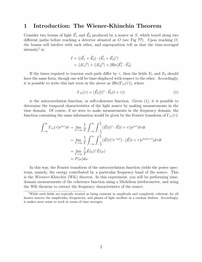
Consider two beams of light ~E1 and ~E2 produced by a source at S, which travel along twodifferent paths before reaching a detector situated at O (see Fig ??). Upon reaching O,the beams will intefere with each other, and superposition tell us that the time-averagedintensity1 is:

I = 〈( ~E1 + ~E2) · ( ~E1 + ~E2)∗〉

= 〈|E1|2〉+ 〈|E2|2〉+ 2Re〈 ~E∗1 · ~E2〉

If the times required to traverse each path differ by τ , then the fields E1 and E2 shouldhave the same form, though one will be time-displaced with respect to the other. Accordingly,it is possible to write this last term in the above as 2Re(Γ11(τ)), where

Γ11(τ) = 〈 ~E1(t)∗ · ~E1(t+ τ)〉 (1)

is the autocorrelation function, or self-coherence function. Given (1), it is possible todetermine the temporal characteristics of the light source by making measurements in thetime domain. Of course, if we were to make measurements in the frequency domain, thefunction containing the same information would be given by the Fourier transform of Γ11(τ):∫ ∞

−∞Γ11(τ)eiωτdτ = lim

T→∞

1

T

∫ ∞−∞

∫ T2

−T2

( ~E(t)∗ · ~E(t+ τ))eiωτdτdt

= limT→∞

1

T

∫ ∞−∞

∫ T2

−T2

( ~E(t)∗e−iωt) · ( ~E(t+ τ)eiω(t+τ))dτdt

= limT→∞

1

TE(ω)∗E(ω)

= P (ω)dω

In this way, the Fourier transform of the autocorrelation function yields the power spec-trum, namely, the energy contributed by a particular frequency band of the source. Thisis the Wienner-Khinchin (WK) theorem. In this experiment, you will be performing time-domain measurements of the coherence function using a Michelson inteforometer, and usingthe WK theorem to extract the frequency characteristics of the source.

1While such fields are typically treated as being constant in amplitude and completely coherent, for allknown sources the amplitudes, frequencies, and phases of light oscillate in a random fashion. Accordingly,it makes more sense to work in terms of time averages.

2

Figure 1: A schematic of the experimental apparatus.

2 Apparatus

2.1 Description of setup

The introduction was motivated by considering the intensity of two beams of light that weremade to interfere after traversing different paths, and it was shown that this can reveal agood deal of information about the source employed. An instrument which performs thisdivision and recombination of the source light is called an inteferometer, and the interferencepattern is recorded in an inteferogram. In this experiment you will be using a MichelsonInterformeter (see fig 1) (the most common configuration), which uses a beam splitter tocreate the optical paths. In the first, the light propagates across a fixed length Lfix, andbounced by mirrors into a detector2. For the other beam, the length of the path (Lmob)is controlled by a mirror mounted on a movable stage, which is translated on the order ofmicrons by a stepper motor. Accordingly, there is a time difference between the two paths:

τ =2(Lmob − Lfix)

c(2)

2For the light sources, mirrors, and scales employed, the process of reflection does not skew the amplitudeor frequency characteristics of the source, to a good approximation.

3

So that, again, by superposition, and by the fact that the two beams are produced bythe same source, the Intensity measured at the detector is:

I(τ) = 2〈I〉+ Re〈Γ11(τ)〉 (3)

As the path is adjusted, the intensity changes, though the time-averaged intensities ofthe light beams 〈I〉 are not altered. In such a way, by determining the intensity at τ = 0, thisvalue can be subtracted from the full I(τ) to isolate the contribution of Γ12(τ). For differentvalues of τ , this information is collected in an inteferogram, which, via the Wiener-Khinchintheorem, may then be used to compute the power spectrum of the incident light sample.

4

Component Description

HeNe Laser

• Source of red lased light, with awell defined peak at 630 nm

• Used to callibrate data andcorrect noise from non-constantstepper velocity

Piezo Controller

• Allows extremely fine control overplacement of movable mirror

Table 1: Component list

5

Component Description

OSL1 White Light Source

• Superposition of all wavelengthsin visible spectrum

• Connected to setup with fibre op-tic cable

• Focused through samples to per-form optical spectroscopy

Silicon Detector

• Silicon detector used to measureintensity of incident light

• This experiment contains two:one to acquire inteferograms(with white light), and the otherto correct for deviations fromnon-constant stepper motor.

Translation Stage + Actuator • Responsible for holding and con-trolling motion of movable mirror

• Motion can be controlled withprovided software, or manuallywith onboard controller

• Stepper motor exhibits non-constant velocity, which com-plicates time-domain measure-ments. Data Analysis softwareemploys algorithms to correctthis deviation based on HeNe cal-libration data (see section 4).

Table 2: Component list, cont.

6

Component Description

Actuator Control Box

• Used to manually adjust positionof movable mirror

Sample Holder• Tripod with attached clamp used tohold sample filters

Interference filters

• Placed in sample holder to filterwhite light source in experimentalinvestigations.

• Green filter used to find zeropoint, as the light filtered with itis brightest among the filters.

Relay lenses, beam spliiters, and mirrors

• Steer beams to determine opticalpath

• It is essential that the laser/-light in this experiment is alignedproperly, otherwise fringes can-not be obtained. Given this, wehighly advise against the positionof these pieces on the table. Ifadjustment is needed, please con-tact the lab technicians.

Table 3: Component list, cont.7

3 Experimental Procedure

3.1 The HeNe Laser

1. Use the alignment procedures (section 4.1) to align the setup for the HeNe light. Makesure you align at when the arm distance difference is zero.

2. Use the Data Acquisition procedures (section 4.2) to set up data acquisition for one ofthe detectors. For the HeNe part of the experiment, you only need one detector.

3. Make sure the output of the interferometer hits one of the detector through the pinhole in the aluminum foil.

4. Before recording the actual data, set up the motor control using the Motor ControlProcedures (see secton 4.3).

5. Set the actuator to move about 1mm or more (However, if you move the actuator toofar, your alignment will deviate since it is difficult to align the setup for all positions).Do not move the detector just yet by pressing Enter.

6. Record the data and while it is recording, quickly go back to the actuator control andmove the actuator by pressing Enter.

7. After the stop recording the data when the actuator is stopped.

8. The recorded data can be found in the Logs section in the Signal Express software.Right click the individual data streams (usually named filtered data, filtered data1)to open their file location in Windows. The files can be opened only with Excel, soremember to save them as .xlsx or any compatible format if planning on analyzing thedata later. Isolate the points corresponding to the interference pattern and create twofiles with the data points from both detectors. Note: It is important that there is aone-to-one correspondence between the HeNe data and the data for the light underexamination in order for the phase correction software to work properly.

9. Use the matlab program to take the FFT of the data to assess the quality of the data.

3.2 White Light

1. Finding the zero point

• To observe interference fringes for broadband light such as the white light, youneed to set the two arm length distance to be exactly equal within few micron oftolerance. (Why ?)

• To find the position of the actuator where the broadband interference fringes canbe observed, first, carefully measure the distance of each arm length using anelectronic caliber. (Warning: Make sure you do not touch any surface of themirrors or the beam splitter cubes with your fingers. Also make sure the calibersdo not scrape any surfaces)

8

• After recoding down the positions, move the actuator so that the arm distancesare roughly the same.

• Using the HeNe light only, adjust the setup at this position using the Alignmentprocedures. The alignment for the HeNe light should also align the setup for thebroadband light source.

• Turn off the HeNe light and turn on the Broadband light source. To see theinterference fringes for this light source, use the J-Jog feature of the actuatorcontroller, or the controller software and move the actuator around the expectedzero difference position. The actuator provides upto 50nm step size for each J-Jogbutton press, depending on your specified J-Jog distance.

• As you do this, you should be able to see interference fringes for the broadbandlight source if you put a piece of white paper like you did in the alignment proce-dure section.

• Now, use the Alignment Procedures again to align for the broadband light thistime. Use the procedure with the broadband light only.

• Make sure the alignment is good across all positions where the interference can beobserved. (Note, the position where the interference fringes are the brightest iswhere the difference in the two arm of the interferometer is exactly zero. Howeverthis is not always true, why ?).

2. Detector setup

• Now you have finished alignment of the setup, its time to set up the detectors.

• Turn on the HeNe laser light and the Broadband light.

• The output of the interferometer should split into two beams of light at the lastbeamsplitter cube after the focal lens.

• For the HeNe light detection, put the detector on the right side of the beamsplittercube such that the ONLY HeNe light dot hits the detector at the pinhole.

• For the Broadband light, put the detector on the bottom of the beamsplitter cubesuch that Only the broadband light dot hits the detector at the pinhole.

• This ensures that each detector reads light from individual light source indepen-dently.

• (Note: If the interference signal is weak when you take data, try narrowing thelight dots by moving the detectors backwards and forwards. This should focusmore light into the pinhole for improved intensity)

3. Running and measuring data

• About 0.5mm away from your measured position where the arm length differenceis zero.

9

• Go to the actuator controller software, set the actuator to move about 1mm. Thisshould scan all range of the interferogram. However, do not move the actuatorjust yet.

• Use the procedures for the data acquisition to acquire data for both detectors(Note, record the data that is filtered using the recommended digital filters)

• Press record and afterwards quickly move the actuator to your specified position.

• Once the actuator stops moving, stop recording the data.

4. Pre-analysis

• In the acquired data, you should crop the regions where there is actual interferencefor both detector signals (Why ? Hint: Alignment). (When you crop the data,make sure you crop both HeNe and broadband light data at the same places intime, and make sure that they have the same number of data points)

• Analyze the interferograms using the Matlab code and obtain the spectrum of thelight under examination.

4 Using the equipment

4.1 Alignment

A NOTE TO THE STUDENT: The equipment used here is extremely sensitive to thealignment (in that it has been built to sense sub-micron changes in position). Please donot remove anything that is bolted to the bench. If you suspect that there is an issue withalignment that is beyond small tweaks, do not fix it yourself. If disturbed, the process ofrealignment is both arduous and highly time-consuming. Please contact the lab techniciansinstead.

• Begin by switching on the HeNe laser. Ensure that all other light sources are switchedoff (it is advised you do this in a dark room).

• Place a white screen (a white piece of paper serves well) between the beam splitter andthe focusing lens.

• If there is no apparent interference pattern, check the position of each output lightthrough the interferometer by blocking each light path.

• By doing this, try to adjust the interferometer mirrors using the adjustment knobs atthe back such that the position for each light output is the same.

• From here, adjust mirrors carefully using the adjustment knobs until you observe in-terference fringes

10

• Adjust the mirror screws and move until getting the widest possible circular interferencepatterns. (Tip. Move the screws in the direction that it gives you wider spacingbetween two consecutive fringes. As you do this, the fringes become more and morecurved. Since the central fringe is bigger than the beam splitter cube in use, if alignedperfectly, you should be able to see rectangular uniform intensity background. Dothe practice alignment exercise below to get a sense of how to do alignment for thisexperiment)

1. Since seeing the circular fringe is difficult when the distances of the two arms areequal, move the actuator so that the difference in this distance is about 1cm. (Thefield of view of the interference pattern should increase as the distance differencebetween the arms increase. Why ? This means that you should be able to seemore fringes per area as the distance difference increase)

2. Now use the alignment tip mentioned above to make sure that the interferencepattern is circular. As you do this, make sure that the circular interference patternis centered with respect to the shadow of the rectangular beam splitter cube.

3. To help you with very fine alignment, turn on the piezo controller and use theX,Y,Z knobs to center the circular interference pattern with respect to the shadowof the cube.

4. At the end, you should be able to see many concentric circular fringes that is thecharacteristic of a Michelson Interferometer. (Why do you see circular fringes ?)

5. Basically, you are trying to do the same thing when the difference in the distanceof the two arms of the interferometer is zero. Except it would be harder to getthe feel of alignment since the central circular fringe will take up the entire fieldof view.

• Set the arm distance such that the difference is zero. Use the same approach toalignment as the practice procedure above.

• Once everything is aligned, take away the sheet of paper that you used to make wayfor the light.

4.2 Data Acquisition

1. Use the ”Signal Express” program

• Click Add Step

→ Acquire Signal

→DAQmx Acquire

→ Analog input

→ Voltage

• Choose the aio and ai1 channels

• Click on Step Setup and scroll to the Timing Settings

11

• Set the following:

→ Acquisition Mode: Continuous Samples

→ Samples to read: 1 K

→ Rate: 10 K

• Press on the DataView tab

• Click Run

• Expand DAQmx Acquire

2. Setting up Digital Filter in Data Acquisition:

• Drag Dev ai0 channel into the window channel. You should now be able to observesome signal.

• In order to isolate the noise software based filters can be applied to the signals:

Press on Add Step

Signal Processing

Analog Signals

Filters

• Customize the filter specifications through the tool box. The following filters arerecommended:

(a) For the ai0 channel (Detector Type: DET36A): (This filter is recommendedfor the HeNe light source)i. Specify input data for the filter: ai0ii. Type: IIR Butterworth Bandstop Filteriii. Upper and Lower cutoffs based on the frequency of noise. E.g. 60Hz noisewould need a bandstop of 50-70Hz

(b) For the ai1 channel (Detector Type: PDA36A): (This filter is recommendedfor the Broadband light source)i. Specify input data for the filter: ai1ii. Type: IIR Butterworth Lowpass Filteriii. Cutoff: 200 Hz

• Add two new displays and drag the two filtered data outputs to the displays.

3. Acquiring data: To record the data, click on the Record button next to the Add Stepbutton. This opens up a pop-up window where the data channels to be recorded canbe selected, as well as the name of the record and an optional description.

4.3 Motor Control

• Setup

Goto: Start Menu → All Programs → Thorlabs → APT → APT User

12

• Set the following settings:

Max. Velocity: 0.05 mm/s

Step Distance: 0.002 mm

Jogging: Single Step

• Operating:

1. Click the position display window, a pop up will show up that asks for the positionin millimeters you want the actuator to be in.

2. Specify the position and press Enter. This should move the actuator with thevelocity specified in the settings.

3. (Warning: if you try to move to a position that exceeds the physical limits of theactuator, the software will give you warnings)

5 Analyzing data

A code is provided to the student to analyze the data using Matlab. The code is quiteinvolved. Do not use the code as a black-box. An essential step in understanding theexperiment is to go through the code and identify the analysis process.

This code uses data provided by the user for the intensity of the light being examinedand data for the HeNe laser taken at the same time by the two detectors. Due to the non-constant speed of the stepper-motor, and the need for the data to be taken at constant phaseintervals, one cannot just Fourier transform the obtained data without modification.

With this in mind, the code does two things: a) It accounts for the non-constant velocityby comparing the data of the examined light with the HeNe data and then creates a vectorof new data points corresponding to points at constant phase intervals. b) It performs a FastFourier Transform

As the data is taken in time domain and the motor moves at a non-constant speed the datafor the HeNe laser deviates from a sinusoidal by being narrower or wider between differentzero crossings. By assuming a phase of pi between consecutive zero crossings one can assignphases to the data obtained and in this way one can then take data points corresponding toconstant phase intervals.

One then performs a discrete Fourier-transform on the data to obtain the power spectraof the examined light.

A more detailed description of the code can be found in appendix III. To run youranalysis, simply specify the file path to your data in the provided code.

6 Questions

1. Before beginning the experiment, trace out the path the light will follow on the bench.

2. Explain why changing the path difference does not change the brightness of the fringesfor the HeNe laser, but it does for non-coherent sources (e.g. white/filtered whitelight).

13

3. The fringes in the Michelson interferometer are called fringes of equal inclination. Whatdoes the term equal inclination refer to?

4. Prove the Convolution theorem. Namely, given a function h(ξ) =∫f(x)g(ξ− x)dx

(the convolution of f and g), its Fourier transform is given by h(k) = f(k)g(k). Use thisto show that the Fourier Transform of Γ11(τ) does indeed yield the power spectrum.

5. In the case of a perfectly monochromatic beam with E(t) = E0e−iω0t, find the form of

Γ11(τ), and P (ω). Is this what you would expect? Why?

6. A more realistic coherence function is given by Γ11(t) = |E0|2e−iω0τe−l0τc , where l0 is the

coherence length of the source (i.e. a length characterizing the decay of the coherencefunction). Show that the resulting Power Spectrum is a Lorentzian centered on ω = ω0,with FWHM l0

c.

7. Use the previous result to compute the coherence length of the red light.

8. Show that for a filter who transmission curve is either a rectangle or triangle with aFWHM of Λ, the interferogram will have its first node for a path difference:

δ =λ20∆λ

Where λ0 is the central wavelength of the transmission curve.

From one of your interferograms, find δ at the first node in terms of λ0 (that is, thenumber of rapid oscillations) and hence determine ∆λ. How does this value comparewith your FT data?

References

[1] Eugene Hecht, Optics. Addison-Wesley 4th Edition 2001

[2] Henry van Driel, Modern Optics and Laser Physics. Rev. 1.7B 1996

[3] Steven W. Smith, The Scientists and Engineer’s Guide to Digital Signal Processing.www.dspguide.com

[4] J. F. James, A Student’s Guide to Fourier Transforms: With Applications to Physicsand Engineering. Cambridge University Press 2nd edition 2002

[5] P. Hariharan Optical Inteferometry Academic Press 2nd edition 2003

[6] For device specifications, go to www.thorlabs.com, or ask the Lab Technicians for thedevice manuals.

14

Appendix I: Sample spectra

Figure 2: Spectrum obtained for white light passed through a red filter

Appendix II: Additional Background on the Fourier Trans-

form

The idea behind the Fourier transform is to represent a function as a sum of waves. To pic-ture this physically, one recalls the principle of superposition. Here, when the two waves aremade to interact, their waveforms are summed, resulting in constructive interference wherethey have the same sign, and destructive interference when they have opposite sign. In sucha way, for a function defined in an interval 0 < x < L, we can represent it as a sum of basicwaveforms (a Fourier series):

f(x) =∞∑n=0

anei2πnxL (4)

where the an are the amplitudes of the nth wave.

15

Figure 3: Partial fourier sums for f(x) = x2

The trouble with using a discrete sum is that we are limited to functions which areperiodic, or are defined within a finite region. To accomodate the full range of functions3,we allow the wavelength to take on continuous values. Defining the wavenumber k = 2π

λ, the

sum becomes an integration over k:

f(x) =

∫ ∞−∞

eikxf(k)dk (5)

It also possible to perform the reverse operation. That is, given a function f(x), we canfind the amplitudes f(k) as:

f(k) =

∫ ∞−∞

e−ikxf(x)dt (6)

In such a way, the function f(k) contains the same amount of information as f(x) - theyare complimentary descriptions, existing in different domains. Whereas f(x) describes theintensity of a signal at a point in the ”space domain”, the fourier transform f(k) describesthe amplitude from a particular point in the ”wavelength domain.”

In the experiment, the characteristic frequencies, that is, the peaks in the spectra, willappear as peaks in f(k).

3There is a good deal of mathematical subtlety we are ignoring here, but for the purpose of this lab allsignals can be fourier transformed

16

Appendix III:

- Importing intensity data for the light under examination and the HeNe laser. Of course, the student needs to change the paths to the files containing obtained data.

W_intensity = importdata('path\to\sample_data.txt');L_intensity = importdata('path\to\hene_data.txt'); - Subtract the average of the intensities to make the oscillations around 0W_avg = mean(W_intensity);W_intensity = W_intensity ­ mean(W_intensity);L_avg = mean(L_intensity);L_intensity = L_intensity ­ mean(L_intensity); -Searching for the zero point crossings - First look for exact zeros (Laser Light)ind0_L = find( L_intensity == 0 ); -> Now ind_0_L contains the indices of the HeNe points that have intensity value 0 - Then look for zero crossings between data points (Laser Light), the idea is that we are multiplying every point with the next point. Since we made the curves oscillate around zero the resulting value would be negative if the zero point has been crossed.L1 = L_intensity(1:end­1) .* L_intensity(2:end);ind1_L = find( L1 < 0 ); -> Now ind_1_L contains the indices of negative values that are followed by positive ones or vice versa- Bring exact zeros and "in-between" zeros together and order them in one vector (Laser Light)ind_L = sort([ind0_L ind1_L]);-> Now ind_L contains the indices of points which have intensity value of exactly zero and for each zero crossing the index for the point right below or above the crossing - Get "fractional" numbers of sample points at which the zeroes are estimated to occur through linear interpolation. There are quite a few subtleties in this function because many cases are being handled. - If the point index in ind_L corresponds to an exact zero no change is madefor (i=1:length(ind_L))

if (L_intensity(ind_L(i))==0)ind_L(i)=ind_L(i);

- But if the point in ind_L lies behind the zero crossing then we linear interpolate to find the index for the zero crossing which would a fractional number. There are two cases to be handled. The point lying behind the zero crossing could be negative or positve.

elseif (L_intensity(ind_L(i))<0 && L_intensity(ind_L(i)+1)>0)            ind_L(i)=ind_L(i)+(abs(L_intensity(ind_L(i))))/(abs(L_intensity(ind_L(i)))+abs(L_intensity(ind_L(i)+1))); elseif (L_intensity(ind_L(i))>0 && L_intensity(ind_L(i)+1)<0)ind_L(i)=ind_L(i)+(abs(L_intensity(ind_L(i))))/(abs(L_intensity(ind_L(i)))+abs(L_intensity(ind_L(i)+1))); - But if the point in ind_L lies after the zero crossing then we linear interpolate to find the index for the zero crossing which would a fractional number. There are two cases to be handled. The point lying after the zero crossing could be negative or positve. elseif (L_intensity(ind_L(i))<0 && L_intensity(ind_L(i)­1)>0)ind_L(i)=ind_L(i)­(abs(L_intensity(ind_L(i))))/(abs(L_intensity(ind_L(i)))+abs(L_intensity(ind_L(i)­1)));elseif (L_intensity(ind_L(i))>0 && L_intensity(ind_L(i)­1)<0)ind_L(i)=ind_L(i)­(abs(L_intensity(ind_L(i))))/(abs(L_intensity(ind_L(i)))+abs(L_intensity(ind_L(i)­1)));

endend -> Now ind_L is expected to contain "mainly" non-integer indices of the points corresponding to zero point crossings - Now we assign phases to all points lying between the first zero crossingand the last zero crossing. The ceil function rounds up any non-integer values. first=ceil(ind_L(1));last=ceil(ind_L(end))­1;

- Initiate a vector of associated phases and set them all to zero. We assign a phase of zero to the first zero crossing and then assume there’s a pi phase difference between consecutive zero crossing and assign the phases to all the obtained data accordingly. This function contains quite afew subtleties as it handles many cases.

L_phase = zeros([1,last­first+1]);

-The index i runs over the points obtained and the index j keeps track of the index values of the zero point crossings.

-A phase value is assigned to the point if it lies between two zero crossings. A pi- phase is always assumed between consecutive zero crossings.for (j=2:length(ind_L))   for (i=first:last)   if (i>ind_L(j))    j=j+1;

   break end               if (i>=ind_L(j­1) && ind_L(j)>=i)         if (ind_L(j­1)>i­1 && i ~= first)               L_phase(i­first+1)= L_phase(i­first)+((i­ind_L(j­1))/(ind_L(j)­ind_L(j­1)))*pi+((ind_L(j­1)­(i­1))/(ind_L(j­1)­ind_L(j­2)))*pi;         elseif (ind_L(j­1)>i­1 && i == first)               L_phase(i­first+1)= L_phase(i­first+1)+((i­ind_L(j­1))/(ind_L(j)­ind_L(j­1)))*pi;                         elseif (ind_L(j­1)<=i­1)               L_phase(i­first+1)= L_phase(i­first)+(1/(ind_L(j)­ind_L(j­1)))*pi;         end       end      end     end -> Now L_phase should contain the phases of all data points - Define segments of equal phase-Phase vector is the same length as the actual intensity vector (between the first and last zero crossing) to prevent FFT problems phases=linspace(L_phase(1), L_phase(end),length( W_intensity (first:last))); -Fit points using cubic spline interpolation (White Light) New_W_intensity = W_intensity (first:last);W_proper=spline(L_phase,New_W_intensity,phases);-> Now W_proper contains data points corresponding to equal phase intervals. It has the same length as the original intensity vector between the first and last zero crossing.

Fourier Transform Part -We set the values to be Fourier transformed equal to the variable I and make it oscillate around 0I = W_proper;  I_avg = mean(I); I = I ­ mean(I); -Set fs to ½ the sample rate in units of Hz-Set V equal to the motor speed in mm/s-The nyquist frequency is ½ the sampling rate. It is the highest frequency that can be coded at a given sampling rate in order to be able to fully reconstruct the signal. It is defined here in THz.

-Frequencies between 0 THz and 100 THz are windowed out fs = 5000; T = 1/fs; V = 0.0499942e­3; D = T*V; Tao = D/3e8; fs_tao = 1/Tao; nyquist = fs_tao/(2*1e12); - m is equal to the window length- n is equal to the length of the vector containing the transformed points- y contains the points that are Fourier transformed- nm is the wavelength range in nm- f is the frequency in THz- power is the the normalized power spectrum to be plotted

m = length(I);           n = pow2(1.5*nextpow2(m))  

 y = fft(I,n);            f = (­n/2:n/2­1)*(fs_tao/n)/1e12;      nm = (1./(f*1e12))*3e8*1e9;   power = abs(y)/n;    power = power/max(power); -Plotting the data

subplot(2,1,1); plot(I); xlabel('Bin'); ylabel('Intensity(V)'); title('Intensity(V) vs Bin: White light filter, Fs = 10kHz'); subplot(2,1,2); plot(nm,fftshift(power)); axis([200 900 0 1]); xlabel('Wavelength (nm)'); ylabel('Transmission'); title('Transmission vs Wavelength (nm)');