advanced topics in computer architecture - marenglen … · 09/04/2010 unyt-uog advanced topics in...

09/04/2010 UNYT-UoG

Advanced Topics in Computer Architecture

Marenglen BibaDepartment of Computer ScienceUniversity of New York Tirana

09/04/2010 UNYT-UoG

Computer Architecture: A Classic• “What do the following have in common: Beatles’ tunes, HP

calculators, chocolate chip cookies, and Computer Architecture? They are all classics that have stood the test of time.”

Robert P. Colwell, Intel lead architect

09/04/2010 UNYT-UoG

Goals of the courseUnderstanding the design techniques, machine structures, technology factors, evaluation methods that will determine the form of computers in 21st Century

09/04/2010 UNYT-UoG

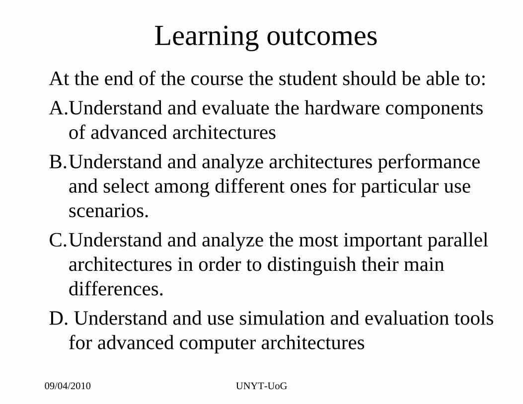
Learning outcomesAt the end of the course the student should be able to:A.Understand and evaluate the hardware components

of advanced architecturesB.Understand and analyze architectures performance

and select among different ones for particular use scenarios.

C.Understand and analyze the most important parallel architectures in order to distinguish their main differences.

D. Understand and use simulation and evaluation tools for advanced computer architectures

09/04/2010 UNYT-UoG

Content• Fundamentals of Computer Design• Pipelining• Instruction-Level Parallelism• Multiprocessors and Thread-Level Parallelism• Interconnection networks for parallel machines• RISC Machines (throughout the course)

09/04/2010 UNYT-UoG

Assessment

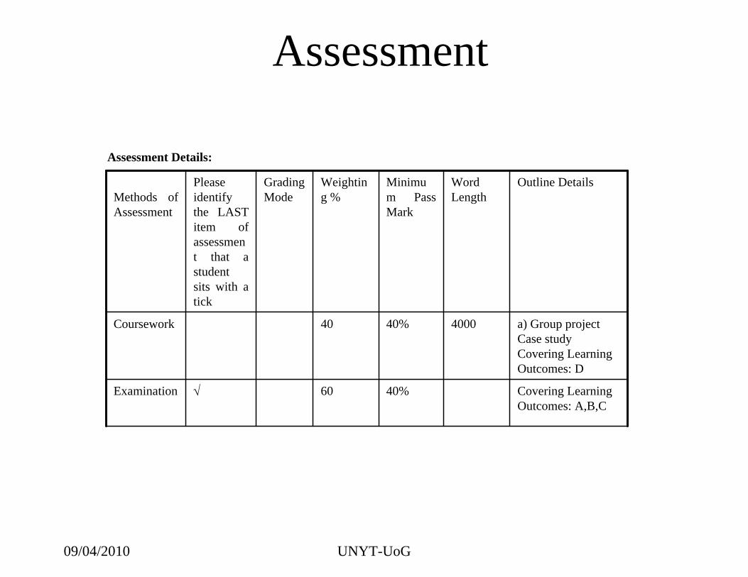
Assessment Details:

Covering Learning Outcomes: A,B,C

40%60Examination

a) Group projectCase studyCovering Learning Outcomes: D

400040%40Coursework

Outline DetailsWord Length

Minimum Pass Mark

Weighting %

Grading Mode

Please identify the LAST item of assessment that a student sits with a tick

Methods of Assessment

09/04/2010 UNYT-UoG

Text

Morgan Kaufmann Publishers

Computer Architecture: A Quantitative Approach, 4th Ed.

2006Hennessy & Patterson

978-0123704900

PublisherTitleDateAuthorISBN Number

09/04/2010 UNYT-UoG

Advanced Topics in Computer Architecture

Lecture 1Fundamentals of Computer Design

Marenglen BibaDepartment of Computer ScienceUniversity of New York Tirana

09/04/2010 UNYT-UoG

Outline1.1 Introduction1.2 Classes of Computers1.3 Defining Computer Architecture1.4 Trends in Technology1.5 Trends in Power in Integrated Circuits1.6 Trends in Cost1.7 Dependability1.8 Measuring, Reporting, and Summarizing

Performance1.9 Quantitative Principles of Computer Design1.10 Putting It All Together: Performance and Price-

Performance1.11 Fallacies and Pitfalls

09/04/2010 UNYT-UoG

Computer Technology• Computer technology has made incredible progress

in the roughly 60 years since the first general-purpose electronic computer was created.

• Today, less than $500 will purchase a personal computer that has more performance, more main memory, and more disk storage than a computer bought in 1985 for 1 million dollars.

• This rapid improvement has come both from advances in the: – technology used to build computers– innovation in computer design.

09/04/2010 UNYT-UoG

Microprocessor• Although technological improvements have been

fairly steady, progress arising from better computer architectures has been much less consistent.

• During the first 25 years of electronic computers, both forces made a major contribution, delivering performance improvement of about 25% per year.

• The late 1970s saw the emergence of the microprocessor.

• The ability of the microprocessor to ride the improvements in integrated circuit technology led to a higher rate of improvement—roughly 35% growth per year in performance.

09/04/2010 UNYT-UoG

Successful Architectures• Two significant changes in the computer marketplace

made it easier than ever before to be commercially successful with a new architecture. – First, the virtual elimination of assembly language

programming reduced the need for object-code compatibility.

– Second, the creation of standardized, vendor-independent operating systems, such as UNIX and its clone, Linux, lowered the cost and risk of bringing out a new architecture.

09/04/2010 UNYT-UoG

RISC Machines• These changes made it possible to develop

successfully a new set of architectures with simpler instructions, called RISC (Reduced Instruction Set Computer) architectures, in the early 1980s.

• The RISC-based machines focused the attention of designers on two critical performance techniques – the exploitation of Instruction level parallelism initially

through pipelining and later through multiple instruction issue

– the use of caches (initially in simple forms and later using more sophisticated organizations and optimizations).

09/04/2010 UNYT-UoG

RISC: Faster Machines• The RISC-based computers raised the performance

bar, forcing prior architectures to keep up or disappear. – The Digital Equipment Vax could not, and so it was

replaced by a RISC architecture. – Intel rose to the challenge, primarily by translating x86

(or IA-32) instructions into RISC-like instructions internally, allowing it to adopt many of the innovations first pioneered in the RISC designs.

• As transistor counts soared in the late 1990s, the hardware overhead of translating the more complex x86 architecture became negligible.

09/04/2010 UNYT-UoG

Uniprocessor performance: 50% Annual Growth until 2002

What is happening?

09/04/2010 UNYT-UoG

The end of an era• The 16-year renaissance is over. • Since 2002, processor performance improvement has

dropped to about 20% per year due to the triple hurdles of: – maximum power dissipation of air-cooled chips, – little instruction-level parallelism left to exploit efficiently, and – almost unchanged memory latency.

• Indeed, in 2004 Intel canceled its high-performance uniprocessor projects and joined IBM and Sun in declaring that the road to higher performance would be via multiple processors per chip rather than via faster uniprocessors.

• This signals a historic switch from relying solely on instruction level parallelism (ILP), to thread-level parallelism (TLP) and data-level parallelism (DLP).

09/04/2010 UNYT-UoG




09/04/2010 UNYT-UoG

Classes of Computers

09/04/2010 UNYT-UoG

Desktop Computing• The first, and still the largest market in dollar terms, is

desktop computing. • Desktop computing spans from low-end systems that sell for

under $500 to high-end, heavily configured workstations that may sell for $5000.

• Throughout this range in price and capability, the desktop market tends to be driven to optimize price-performance.

• This combination of performance (measured primarily in terms of compute performance and graphics performance) and price of a system is what matters most to customers in this market, and hence to computer designers.

• As a result, the newest, highest-performance microprocessors and cost-reduced microprocessors often appear first in desktop systems

09/04/2010 UNYT-UoG

Servers• As the shift to desktop computing occurred, the role of servers grew to

provide larger-scale and more reliable file and computing services. • The World Wide Web accelerated this trend because of the tremendous

growth in the demand and sophistication of Web-based services. • Such servers have become the backbone of large-scale enterprise

computing, replacing the traditional mainframe.• For servers, different characteristics are important. First, dependability is

critical.• Consider the servers running Google, taking orders for Cisco, or running

auctions on eBay. – Failure of such server systems is far more catastrophic than failure of

a single desktop, since these servers must operate seven days a week, 24 hours a day.

• To bring costs up-to-date, Amazon.com had $2.98 billion in sales in the fall quarter of 2005.

• As there were about 2200 hours in that quarter, the average revenue per hour was $1.35 million. During a peak hour for Christmas shopping, the potential loss would be many times higher.

09/04/2010 UNYT-UoG

Cost of downtime (Amazon data)

09/04/2010 UNYT-UoG

Servers: other features• A second key feature of server systems is

scalability. – Server systems often grow in response to an increasing

demand for the services they support or an increase in functional requirements.

– Thus, the ability to scale up the computing capacity, the memory, the storage, and the I/O bandwidth of a server is crucial.

• Lastly, servers are designed for efficient throughput. – That is, the overall performance of the server—in terms

of transactions per minute or Web pages served per second—is what is crucial.

09/04/2010 UNYT-UoG

Supercomputers• A related category is supercomputers. • They are the most expensive computers, costing tens of

millions of dollars, and they emphasize floating-point performance.

• Clusters of desktop computers, have largely overtaken this class of computer.

• As clusters grow in popularity, the number of conventional supercomputers is shrinking, as are the number of companies who make them.

09/04/2010 UNYT-UoG

Embedded Computers• Embedded computers are the fastest growing portion of the

computer market.

• These devices range from everyday machines—most microwaves, most washing machines, most printers, most networking switches, and all cars contain simple embedded microprocessors—to handheld digital devices, such as cell phones and smart cards, to video games and digital set-top boxes.

09/04/2010 UNYT-UoG

Embedded Computers• Embedded computers have the widest spread of processing

power and cost.• They include 8-bit and 16-bit processors that may cost less

than a dime, 32-bit microprocessors that execute 100 million instructions per second and cost under $5, and high-end processors for the newest video games or network switches that cost $100 and can execute a billion instructions per second.

• Although the range of computing power in the embedded computing market is very large, price is a key factor in the design of computers for this space.

• Performance requirements do exist, of course, but the primary goal is often meeting the performance need at minimum price, rather than achieving higher performance at a higher price.

09/04/2010 UNYT-UoG

Embedded Computers and real-time execution

• Often, the performance requirement in an embedded application is real-time execution.

• A real-time performance requirement is when a segment of the application has an absolute maximum execution time.

• For example, in a digital set-top box, the time to process each video frame is limited, since the processor must accept and process the next frame shortly.

• In some applications, a more nuanced requirement exists: the average time for a particular task is constrained as well as the number of instances when some maximum time is exceeded.

09/04/2010 UNYT-UoG




09/04/2010 UNYT-UoG

Defining Computer Architecture• The task the computer designer faces is a complex one:

Determine what attributes are important for a new computer, then design a computer to maximize performance while staying within cost, power, and availability constraints.

• This task has many aspects, including instruction set design, functional organization, logic design, and implementation.

• The implementation may encompass integrated circuit design, packaging, power, and cooling.

• Optimizing the design requires familiarity with a very wide range of technologies, from compilers and operating systems to logic design and packaging.

09/04/2010 UNYT-UoG

Defining Computer Architecture• In the past, the term computer architecture often referred

only to instruction set design. • Other aspects of computer design were called

implementation, often insinuating that implementation is uninteresting or less challenging.

• This view is incorrect. • The architect’s or designer’s job is much more than

instruction set design, and the technical hurdles in the other aspects of the project are likely more challenging than those encountered in instruction set design.

• We’ll review instruction set architecture before describing the larger challenges for the computer architect.

09/04/2010 UNYT-UoG

Instruction Set Architecture• We use the term instruction set architecture (ISA)

to refer to the actual programmer visible instruction set.

• The ISA serves as the boundary between the software and hardware.

• In this quick review of ISA we will use examples from MIPS and 80x86 to illustrate the seven dimensions of an ISA

09/04/2010 UNYT-UoG

MIPS• MIPS (originally an acronym for Microprocessor without

Interlocked Pipeline Stages) is a reduced instruction set computer (RISC) developed by MIPS Computer Systems (now MIPS Technologies).

• The early MIPS architectures were 32-bit, and later versions were 64-bit. Multiple revisions of the MIPS instruction set exist, including MIPS I, MIPS II, MIPS III, MIPS IV, MIPS V, MIPS32, and MIPS64.

• The current revisions are MIPS32 (for 32-bit implementations) and MIPS64 (for 64-bit implementations).

• MIPS32 and MIPS64 define a control register set as well as the instruction set.

09/04/2010 UNYT-UoG

x86 family• The term x86 refers to a family of instruction set architectures

based on the Intel 8086. • The term is derived from the fact that many early processors that

are backward compatible with the 8086 also had names ending in "86".

• Many additions and extensions have been added to the x86 instruction set over the years, almost consistently with full backwards compatibility. The architecture has been implemented in processors from Intel, Cyrix, AMD, VIA and many others.

• As the x86 term became common after the introduction of the 80386, it usually implies binary compatibility with the 32-bit instruction set of the 80386.

• This may sometimes be emphasized as x86-32 to distinguish it either from the original 16-bit x86-16 or from the newer 64-bit x86-64 (also called x64).

09/04/2010 UNYT-UoG

Dimensions of ISAs1. Class of ISA• Nearly all ISAs today are classified as general-purpose

register architectures, where the operands are either registers or memory locations.

• The 80x86 has 16 general-purpose registers and 16 that can hold floating-point data, while MIPS has 32 general-purpose and 32 floating-point registers.

• The two popular versions of this class are: – register-memory ISAs such as the 80x86, which can

access memory as part of many instructions – load-store ISAs such as MIPS, which can access memory

only with load or store instructions. • All recent ISAs are load-store.

09/04/2010 UNYT-UoG

Dimensions of ISAs2. Memory addressing• Virtually all desktop and server computers,

including the 80x86 and MIPS, use byte addressing to access memory operands.

• Some architectures, like MIPS, require that objects must be aligned.– An access to an object of size s bytes at byte address A is

aligned if A mod s = 0. • The 80x86 does not require alignment, but accesses

are generally faster if operands are aligned.

09/04/2010 UNYT-UoG

Dimensions of ISAs3. Addressing modes• In addition to specifying registers and constant operands,

addressing modes specify the address of a memory object. • MIPS addressing modes are Register, Immediate (for

constants), and Displacement, where a constant offset is added to a register to form the memory address.

• The 80x86 supports those three plus three variations of displacement: – no register (absolute), – two registers (based indexed with displacement), – two registers where one register is multiplied by the size

of the operand in bytes (based with scaled index and displacement).

09/04/2010 UNYT-UoG

Dimensions of ISAs4. Types and sizes of operands• Like most ISAs, MIPS and 80x86 support operand sizes of

8-bit (ASCII character), 16-bit (Unicode character or half word), 32-bit (integer or word), 64-bit (double word or long integer), and IEEE 754 floating point in 32-bit (single precision) and 64-bit (double precision).

• The 80x86 also supports 80-bit floating point (extended double precision).

09/04/2010 UNYT-UoG

Dimensions of ISAs5. Operations• The general categories of operations are data

transfer, arithmetic logical, control and floating point.

• MIPS is a simple and easy-to-pipeline instruction set architecture, and it is representative of the RISC architectures being used in 2006.

• The 80x86 has a much richer and larger set of operations and it is representative of the CISC machines.

09/04/2010 UNYT-UoG

MIPS instructions

09/04/2010 UNYT-UoG

Dimensions of ISAs6. Control flow instructions• Virtually all ISAs, including 80x86 and MIPS, support

conditional branches, unconditional jumps, procedure calls, and returns.

• Both use PC-relative addressing, where the branch address is specified by an address field that is added to the PC.

• There are some small differences. – MIPS conditional branches (BE,BNE, etc.) test the

contents of registers, – 80x86 branches (JE,JNE, etc.) test condition code bits as

side effects of arithmetic/logic operations.

09/04/2010 UNYT-UoG

Dimensions of ISAs7. Encoding an ISA• There are two basic choices on encoding: fixed length and

variable length.– All MIPS instructions are 32 bits long, which simplifies

instruction decoding. – The 80x86 encoding is variable length, ranging from 1 to 18

bytes. • Variable-length instructions can take less space than fixed-length

instructions, so a program compiled for the 80x86 is usually smaller than the same program compiled for MIPS.

• Note that choices mentioned above will affect how the instructions are encoded into a binary representation. – For example, the number of registers and the number of

addressing modes both have a significant impact on the size of instructions.

09/04/2010 UNYT-UoG

MIPS ISA formats

09/04/2010 UNYT-UoG

Implementation: Organization and Hardware

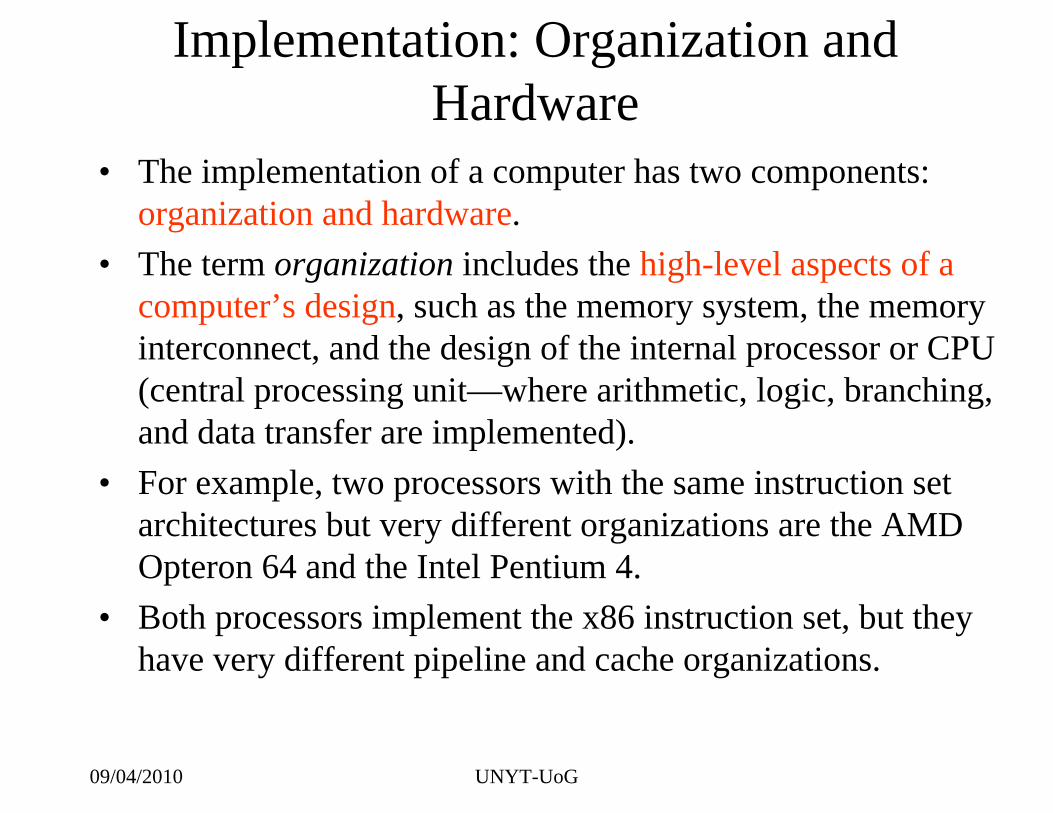
• The implementation of a computer has two components: organization and hardware.

• The term organization includes the high-level aspects of a computer’s design, such as the memory system, the memory interconnect, and the design of the internal processor or CPU (central processing unit—where arithmetic, logic, branching, and data transfer are implemented).

• For example, two processors with the same instruction set architectures but very different organizations are the AMD Opteron 64 and the Intel Pentium 4.

• Both processors implement the x86 instruction set, but they have very different pipeline and cache organizations.

09/04/2010 UNYT-UoG

Hardware• Hardware refers to the specifics of a computer, including the

detailed logic design and the packaging technology of the computer.

• Often a line of computers contains computers with identical instruction set architectures and nearly identical organizations, but they differ in the detailed hardware implementation.

• For example, the Pentium 4 and the Mobile Pentium 4 are nearly identical, but offer different clock rates and different memory systems, making the Mobile Pentium 4 more effective for low-end computers.

09/04/2010 UNYT-UoG

Defining Computer Architecture• In this course, the word architecture covers all three

aspects of computer design:– instruction set architecture – organization – hardware.

09/04/2010 UNYT-UoG

Computer Design Requirements• Computer architects must design a computer to meet:

– functional requirements as well as – price, power, performance, and availability goals.

• Often, architects also must determine what the functional requirements are, which can be a major task. – The requirements may be specific features inspired by the

market. – Application software often drives the choice of certain

functional requirements by determining how the computer will be used.

– If a large body of software exists for a certain instruction set architecture, the architect may decide that a new computer should implement an existing instruction set.

09/04/2010 UNYT-UoG

Functional Requirements

09/04/2010 UNYT-UoG




09/04/2010 UNYT-UoG

Trends in Technology• If an instruction set architecture is to be successful, it must

be designed to survive rapid changes in computer technology. – After all, a successful new instruction set architecture

may last decades—for example, the core of the IBM mainframe has been in use for more than 40 years.

• An architect must plan for technology changes that can increase the lifetime of a successful computer.– To plan for the evolution of a computer, the designer

must be aware of rapid changes in implementation technology.

• Four implementation technologies, which change at a dramatic pace, are critical to modern implementations:

09/04/2010 UNYT-UoG

1- Integrated circuit logic technology• Transistor density increases by about 35% per year,

quadrupling in somewhat over four years. • Increases in die size are less predictable and slower, ranging

from 10% to 20% per year. • The combined effect is a growth rate in transistor count on a

chip of about 40% to 55% per year. • Device speed scales more slowly

09/04/2010 UNYT-UoG

2- SDRAM• Synchronous DRAM (dynamic random-access

memory) – Capacity increases by about 40% per year,

doubling roughly every two years.

09/04/2010 UNYT-UoG

3- Magnetic disk technology• Prior to 1990, density increased by about 30% per year,

doubling in three years. • It rose to 60% per year thereafter, and increased to 100% per

year in 1996. • Since 2004, it has dropped back to 30% per year. • Despite this roller coaster of rates of improvement, disks are

still 50–100 times cheaper per bit than DRAM.

09/04/2010 UNYT-UoG

4- Network technology• Network performance depends both on the

performance of switches and on the performance of the transmission system.

• Interconnections networks for parallel systems are essential in exploiting parallelism.

09/04/2010 UNYT-UoG

Performance Trends: Bandwidth over Latency

• Bandwidth or throughput is the total amount of work done in a given time, such as megabytes per second for a disk transfer.

• In contrast, latency or response time is the time between the start and the completion of an event, such as milliseconds for a disk access.

• Bandwidth improves much more rapidly than latency => next slide.

09/04/2010 UNYT-UoG

Bandwidth over Latency

09/04/2010 UNYT-UoG

Performance Milestones

09/04/2010 UNYT-UoG

Scaling of Transistor Performance and Wires

• Integrated circuit processes are characterized by the feature size, which is the minimum size of a transistor or a wire in either the x or y dimension.

• Feature sizes have decreased from 10 microns in 1971 to 0.09 microns in 2006; – in fact, we have switched units, so production in 2006

was referred to as “90 nanometers,” and 65 nanometer chips were underway.

• Since the transistor count per square millimeter of silicon is determined by the surface area of a transistor, the density of transistors increases quadratically with a linear decrease in feature size.

09/04/2010 UNYT-UoG

Transistor performance• The increase in transistor performance, however, is more

complex. • As feature sizes shrink, devices shrink quadratically in the

horizontal dimension and also shrink in the vertical dimension.

• The shrink in the vertical dimension requires a reduction in operating voltage to maintain correct operation and reliability of the transistors.

• This combination of scaling factors leads to a complex interrelationship between transistor performance and process feature size.

• To a first approximation, transistor performance improves linearly with decreasing feature size.

09/04/2010 UNYT-UoG

Wires performance• Although transistors generally improve in performance with

decreased feature size, wires in an integrated circuit do not. • In particular, the signal delay for a wire increases in proportion to

the product of its resistance and capacitance. – Of course, as feature size shrinks, wires get shorter, but the

resistance and capacitance per unit length get worse. • This relationship is complex, since both resistance and capacitance

depend on: – detailed aspects of the process, – the geometry of a wire, – the loading on a wire, and – even the adjacency to other structures.

09/04/2010 UNYT-UoG

Wire Delay• In general, wire delay scales poorly compared to

transistor performance, creating additional challenges for the designer.

• In the past few years, wire delay has become a major design limitation for large integrated circuits and is often more critical than transistor switching delay.

• Larger and larger fractions of the clock cycle have been consumed by the propagation delay of signals on wires.

• In 2001, the Pentium 4 broke new ground by allocating 2 stages of its 20+-stage pipeline just for propagating signals across the chip.

09/04/2010 UNYT-UoG




09/04/2010 UNYT-UoG

Trends in Power in Integrated Circuits

• Power also provides challenges as devices are scaled.

• First, power must be brought in and distributed around the chip, and modern microprocessors use hundreds of pins and multiple interconnect layers for just power and ground.

• Second, power is dissipated as heat and must be removed.

09/04/2010 UNYT-UoG

Dynamic Power• For CMOS chips, the traditional dominant energy

consumption has been in switching transistors, also called dynamic power.

• The power required per transistor is proportional to the product of the load capacitance of the transistor, the square of the voltage, and the frequency of switching, with watts being the unit:

Powerdynamic = 1 ⁄ 2 × Capacitive load × Voltage2 × Frequency switched

• Mobile devices care about battery life more than power, so energy is the proper metric, measured in joules:

Energydynamic = Capacitive load × Voltage2

09/04/2010 UNYT-UoG

Dynamic Power• Dynamic power and energy are greatly reduced by

lowering the voltage, and so voltages have dropped from 5V to just over 1V in 20 years.

• The capacitive load is a function of the number of transistors connected to an output and the technology, which determines the capacitance of the wires and the transistors.

• For a fixed task, slowing clock rate reduces power, but not energy.

09/04/2010 UNYT-UoG

Heat dissipation• As we move from one process to the next, the increase in the

number of transistors switching, and the frequency with which they switch, dominates the decrease in load capacitance and voltage, leading to an overall growth in power consumption and energy.

• The first microprocessors consumed tenths of a watt, while a 3.2 GHz Pentium 4 Extreme Edition consumes 135 watts. – Given that this heat must be dissipated from a chip that is

about 1 cm on a side, we are reaching the limits of what can be cooled by air

• Several Intel microprocessors have temperature diodes to reduce activity automatically if the chip gets too hot. – For example, they may reduce voltage and clock

frequency or the instruction issue rate.

09/04/2010 UNYT-UoG

Heat dissipation• Distributing the power, removing the heat, and

preventing hot spots have become increasingly difficult challenges.

• Power is now the major limitation to using transistors; in the past it was raw silicon area.

• As a result of this limitation, most microprocessors today turn off the clock of inactive modules to save energy and dynamic power. – For example, if no floating-point instructions are

executing, the clock of the floating-point unit is disabled.

09/04/2010 UNYT-UoG




09/04/2010 UNYT-UoG

Trends in Cost• Although there are computer designs where costs tend to be

less important — specifically supercomputers — cost-sensitive designs are of growing significance.

• Indeed, in the past 20 years, the use of technology improvements to lower cost, as well as increase performance, has been a major theme in the computer industry.

• Textbooks often ignore the cost half of cost-performance because costs change, thereby dating books, and because the issues are subtle and differ across industry segments.

• Yet an understanding of cost and its factors is essential for designers to make intelligent decisions about whether or not a new feature should be included in designs where cost is an issue.

09/04/2010 UNYT-UoG

Cost of computer manufacturing• The cost of a manufactured computer component

decreases over time even without major improvements in the basic implementation technology.

• The underlying principle that drives costs down is the learning curve — manufacturing costs decrease over time.

• The learning curve itself is best measured by change in yield — the percentage of manufactured devices that survives the testing procedure.

• Whether it is a chip, a board, or a system, designs that have twice the yield will have half the cost.

09/04/2010 UNYT-UoG

Learning curve• Understanding how the learning curve improves yield is

critical to projecting costs over a product’s life. • One example is that the price per megabyte of DRAM has

dropped over the long term by 40% per year. Since DRAMstend to be priced in close relationship to cost — with the exception of periods when there is a shortage or an oversupply — price and cost of DRAM track closely.

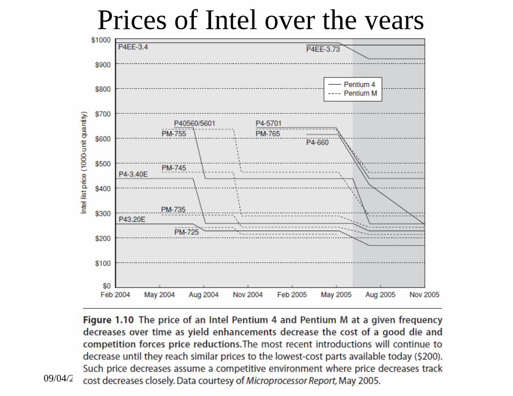
• Microprocessor prices also drop over time, but because they are less standardized than DRAMs, the relationship between price and cost is more complex.

• In a period of significant competition, price tends to track cost closely, although microprocessor vendors probably rarely sell at a loss.

09/04/2010 UNYT-UoG

Prices of Intel over the years

09/04/2010 UNYT-UoG

Cost of an Integrated Circuit• In an increasingly competitive computer marketplace where

standard parts — disks, DRAMs, and so on — are becoming a significant portion of any system’s cost, integrated circuit costs are becoming a greater portion of the cost that varies between computers, especially in the high-volume, cost-sensitive portion of the market.

• Thus, computer designers must understand the costs of chips to understand the costs of current computers.

09/04/2010 UNYT-UoG

Die

09/04/2010 UNYT-UoG

Wafer and dies

09/04/2010 UNYT-UoG

Cost of an Integrated Circuit• Although the costs of integrated circuits have

dropped exponentially, the basic process of silicon manufacture is unchanged: A wafer is still tested and chopped into dies that are packaged. Thus the cost of a packaged integrated circuit is:

09/04/2010 UNYT-UoG

Cost of Dies• Learning how to predict the number of good chips per wafer

requires first learning how many dies fit on a wafer and then learning how to predict the percentage of those that will work. From there it is simple to predict cost:

• The most interesting feature of this first term of the chip costequation is its sensitivity to die size, shown below:

• The number of dies per wafer is approximately the area of the wafer divided by the area of the die. It can be more accurately estimated by:

09/04/2010 UNYT-UoG

Cost of Dies• Processing of a 300 mm (12-inch) diameter wafer in

a leading-edge technology costs between $5000 and $6000 in 2006.

• Assuming a processed wafer cost of $5500, the cost of the 1.00 cm2 die would be around $13, but the cost per die of the 2.25 cm2 die would be about $46, or almost four times the cost for a die that is a little over twice as large.

09/04/2010 UNYT-UoG

What should a computer designer remember about chip costs?

• The manufacturing process dictates the wafer cost, wafer yield, and defects per unit area, so the sole control of the designer is die area.

• In practice, because the number of defects per unit area is small, the number of good dies per wafer, and hence the cost per die, grows roughly as the square of the die area.

• The computer designer affects die size, and hence cost, both by what functions are included on or excluded from the die and by the number of I/O pins.

09/04/2010 UNYT-UoG




09/04/2010 UNYT-UoG

Dependability• Historically, integrated circuits were one of the most reliable

components of a computer. • Although their pins may be vulnerable, and faults may occur

over communication channels, the error rate inside the chip was very low.

• That conventional wisdom is changing as we head to feature sizes of 65 nm and smaller, as both transient faults and permanent faults will become more commonplace, so architects must design systems to cope with these challenges.

09/04/2010 UNYT-UoG

Service Level Agreements• One difficult question is deciding when a system is operating

properly. • This philosophical point became concrete with the popularity

of Internet services.• Infrastructure providers started offering Service Level

Agreements (SLA) or Service Level Objectives (SLO) to guarantee that their networking or power service would be dependable.

• For example, they would pay the customer a penalty if they did not meet an agreement more than some hours per month.

• Thus, an SLA could be used to decide whether the system was up or down.

09/04/2010 UNYT-UoG

Measures of dependability• Systems alternate between two states of service with respect

to an SLA:1. Service accomplishment, where the service is delivered as

specified2. Service interruption, where the delivered service is

different from the SLA• Transitions between these two states are caused by failures

(from state 1 to state 2) or restorations (2 to 1). • Quantifying these transitions leads to the two main measures

of dependability:– Module reliability– Module availability

09/04/2010 UNYT-UoG

Module reliability• Module reliability is a measure of the continuous service

accomplishment (or, equivalently, of the time to failure) from a reference initial instant.

• Hence, the mean time to failure (MTTF) is a reliability measure.

• The reciprocal of MTTF is a rate of failures, generally reported as failures per billion hours of operation, or FIT (for failures in time).

• Thus, an MTTF of 1,000,000 hours equals 109⁄ 106 or 1000 FIT.

• Service interruption is measured as mean time to repair (MTTR).

• Mean time between failures (MTBF) is simply the sum ofMTTF + MTTR.

09/04/2010 UNYT-UoG

Module availability• Module availability is a measure of the service accomplishment

with respect to the alternation between the two states of accomplishment and interruption.

• For nonredundant systems with repair, module availability is:

• Note that reliability and availability are now quantifiable metrics, rather than synonyms for dependability.

• From these definitions, we can estimate reliability of a system quantitatively if we make some assumptions about the reliability of components and that failures are independent.

09/04/2010 UNYT-UoG

Example• Assume a disk subsystem with the following

components and MTTF:– 10 disks, each rated at 1,000,000-hour MTTF– 1 SCSI controller, 500,000-hour MTTF– 1 power supply, 200,000-hour MTTF– 1 fan, 200,000-hour MTTF– 1 SCSI cable, 1,000,000-hour MTTF

• Using the simplifying assumptions that the lifetimes are exponentially distributed and that failures are independent, compute the MTTF of the system as a whole.

09/04/2010 UNYT-UoG

Example

09/04/2010 UNYT-UoG

Quantifying performance• Having quantified the cost, power, and

dependability of computer technology, we are ready to quantify performance.

09/04/2010 UNYT-UoG




09/04/2010 UNYT-UoG

Measuring Performance• When we say one computer is faster than another, what do

we mean? • The user of a desktop computer may say a computer is faster

when a program runs in less time, while an Amazon.comadministrator may say a computer is faster when it completes more transactions per hour.

• The computer user is interested in reducing response time— the time between the start and the completion of an event also referred to as execution time.

• The administrator of a large data processing center may be interested in increasing throughput — the total amount of work done in a given time.

09/04/2010 UNYT-UoG

Comparing Alternatives• In comparing design alternatives, we often want to

relate the performance of two different computers, say, X and Y.

• The phrase “X is faster than Y” is used here to mean that the response time or execution time is lower on X than on Y for the given task. In particular, “X is n times faster than Y” will mean:

09/04/2010 UNYT-UoG

Comparing Alternatives• Since execution time is the reciprocal of performance, the

following relationship holds:

• The phrase “the throughput of X is 1.3 times higher than Y” signifies here that the number of tasks completed per unit time on computer X is 1.3 times the number completed on Y.

09/04/2010 UNYT-UoG

Measuring performance• Unfortunately, time is not always the metric quoted

in comparing the performance of computers. • Hennessy & Patterson’s position is that the only

consistent and reliable measure of performance is the execution time of real programs, and that all proposed alternatives to time as the metric or to real programs as the items measured have eventually led to misleading claims or even mistakes in computer design.

09/04/2010 UNYT-UoG

Execution time• Even execution time can be defined in different ways depending

on what we count. • The most straightforward definition of time is called wall-clock

time, response time, or elapsed time, which is the latency to complete a task, including disk accesses, memory accesses, input/output activities, operating system overhead— everything.

• With multiprogramming, the processor works on another program while waiting for I/O and may not necessarily minimize the elapsed time of one program.

• Hence, we need a term to consider this activity. CPU timerecognizes this distinction and means the time the processor is computing, not including the time waiting for I/O or running other programs. (Clearly, the response time seen by the user is the elapsed time of the program, not the CPU time.)

09/04/2010 UNYT-UoG

Benchmarks• The best choice of benchmarks to measure performance are

real applications, such as a compiler. • Attempts at running programs that are much simpler than a

real application have led to performance pitfalls. • Examples include

– kernels, which are small, key pieces of real applications;– toy programs, which are 100-line programs from

beginning programming assignments, such as quicksort; and

– synthetic benchmarks, which are fake programs invented to try to match the profile and behavior of real applications, such as Dhrystone.

09/04/2010 UNYT-UoG

Benchmark-specific flags• Another issue is the conditions under which the benchmarks

are run. • One way to improve the performance of a benchmark has

been with benchmark-specific flags; – these flags often caused transformations that would be

illegal on many programs or would slow down performance on others.

• To restrict this process and increase the significance of the results, benchmark developers often require the vendor to use one compiler and one set of flags for all the programs in the same language (C or FORTRAN).

09/04/2010 UNYT-UoG

Benchmark suites• Collections of benchmark applications, called benchmark

suites, are a popular measure of performance of processors with a variety of applications.

• Of course, such suites are only as good as the constituent individual benchmarks.

• Nonetheless, a key advantage of such suites is that the weakness of any one benchmark is lessened by the presence of the other benchmarks.

• The goal of a benchmark suite is that it will characterize the relative performance of two computers, particularly for programs not in the suite that customers are likely to run.

09/04/2010 UNYT-UoG

EEMBC• The EDN Embedded Microprocessor Benchmark

Consortium (or EEMBC, pronounced “embassy”) is a set of 41 kernels used to predict performance of different embedded applications: automotive/industrial, consumer, networking, office automation, and telecommunications. EEMBC reports unmodified performance and “full fury”performance, where almost anything goes.

• Because they use kernels, and because of the reporting options, EEMBC does not have the reputation of being a good predictor of relative performance of different embedded computers in the field.

09/04/2010 UNYT-UoG

SPEC• One of the most successful attempts to create standardized

benchmark application suites has been the SPEC (Standard Performance Evaluation Corporation), which had its roots in the late 1980s efforts to deliver better benchmarks for workstations.

• Just as the computer industry has evolved over time, so has the need for different benchmark suites, and there are now SPEC benchmarks to cover different application classes.

• All the SPEC benchmark suites and their reported results are found at www.spec.org.

• Although we focus our discussion on the SPEC benchmarks, there are also many benchmarks developed for PCs running the Windows operating system.

09/04/2010 UNYT-UoG

Desktop Benchmark• Desktop benchmarks divide into two broad classes:

– processor-intensive benchmarks and – graphics-intensive benchmarks, although many graphics

benchmarks include intensive processor activity. • SPEC originally created a benchmark set focusing on

processor performance (initially called SPEC89), which has evolved into its fifth generation: SPEC CPU2006, which follows SPEC2000, SPEC95, SPEC92, and SPEC89.

• SPEC CPU2006 consists of a set of 12 integer benchmarks (CINT2006) and 17 floating-point benchmarks (CFP2006).

09/04/2010 UNYT-UoG

SPEC benchmarksSPEC2006 programs and the evolution of the SPEC benchmarks over time, with integer programsabove the line and floating-point programs below the line. Of the 12 SPEC2006 integer programs, 9 are written in C, and the rest in C++. For the floating-point programs the split is 6 in FORTRAN, 4 in C++, 3 in C, and 4 in mixed Cand Fortran.

09/04/2010 UNYT-UoG

Server Benchmarks - 1• Just as servers have multiple functions, so there are multiple

types of benchmarks.• The simplest benchmark is perhaps a processor throughput-

oriented benchmark. • SPEC CPU2000 uses the SPEC CPU benchmarks to

construct a simple throughput benchmark where the processing rate of a multiprocessor can be measured by running multiple copies (usually as many as there are processors) of each SPEC CPU benchmark and converting the CPU time into a rate.

• This leads to a measurement called the SPECrate.

09/04/2010 UNYT-UoG

Server Benchmarks - 2• Most server applications and benchmarks have significant I/O

activity arising from either disk or network traffic, including benchmarks for file server systems, for Web servers, and for database and transaction processing systems.

• SPEC offers both a file server benchmark (SPECSFS) and a Web server benchmark (SPECWeb).

• SPECSFS is a benchmark for measuring NFS (Network File System) performance using a script of file server requests; it tests the performance of the I/O system (both disk and network I/O) aswell as the processor.

• SPECSFS is a throughput-oriented benchmark but with important response time requirements.

• SPECWeb is a Web server benchmark that simulates multiple clients requesting both static and dynamic pages from a server, as well as clients posting data to the server.

09/04/2010 UNYT-UoG

Server Benchmarks - 3• Transaction-processing (TP) benchmarks measure

the ability of a system to handle transactions, which consist of database accesses and updates.

• Airline reservation systems and bank ATM systems are typical simple examples of TP;– more sophisticated TP systems involve complex

databases and decision-making.• In the mid-1980s, a group of concerned engineers

formed the vendor-independent Transaction Processing Council (TPC) to try to create realistic and fair benchmarks for TP.

• The TPC benchmarks are described at www.tpc.org.

09/04/2010 UNYT-UoG

Reporting Performance Results• The guiding principle of reporting performance measurements

should be reproducibility — list everything another experimenter would need to duplicate the results.

• A SPEC benchmark report requires an extensive description of thecomputer and the compiler flags, as well as the publication of both the baseline and optimized results.

• In addition to hardware, software, and baseline tuning parameterdescriptions, a SPEC report contains the actual performance times, shown both in tabular form and as a graph.

• A TPC benchmark report is even more complete, since it must include results of a benchmarking audit and cost information.

• These reports are excellent sources for finding the real cost ofcomputing systems, since manufacturers compete on high performance and cost-performance.

09/04/2010 UNYT-UoG

Summarizing Performance Results• In practical computer design, you must evaluate myriads of

design choices for their relative quantitative benefits across asuite of benchmarks believed to be relevant.

• Likewise, consumers trying to choose a computer will rely on performance measurements from benchmarks, which hopefully are similar to the user’s applications.

• In both cases, it is useful to have measurements for a suite of benchmarks so that the performance of important applications is similar to that of one or more benchmarks in the suite and that variability in performance can be understood.

09/04/2010 UNYT-UoG

Choosing summarizing measures• Once we have chosen to measure performance with a benchmark suite,

we would like to be able to summarize the performance results of the suite in a single number.

• A straightforward approach to computing a summary result would be to compare the arithmetic means of the execution times of the programs in the suite.– But some SPEC programs take four times longer than others, so

those programs would be much more important if the arithmetic mean were the single number used to summarize performance.

• An alternative would be to add a weighting factor to each benchmark and use the weighted arithmetic mean as the single number to summarize performance.

• The problem would be then how to pick weights; since SPEC is a consortium of competing companies, each company might have theirown favorite set of weights, which would make it hard to reach consensus.

09/04/2010 UNYT-UoG

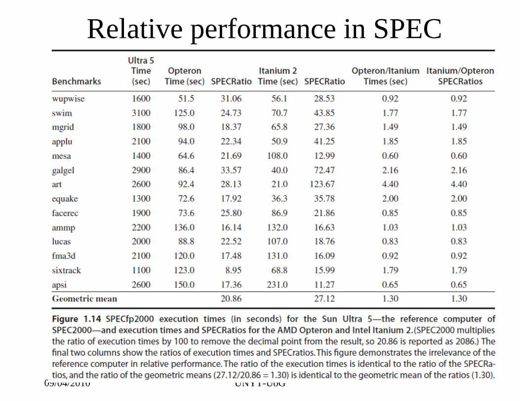
Reference Computer• Rather than pick weights, we could normalize execution times to a

reference computer by dividing the time on the reference computer by the time on the computer being rated, yielding a ratio proportional to performance. – SPEC uses this approach, calling the ratio the SPECRatio.

• For example, suppose that the SPECRatio of computer A on a benchmark was 1.25 times higher than computer B; then you would know

• Notice that the execution times on the reference computer drop out and the choice of the reference computer is irrelevant when the comparisons are made as a ratio, which is the approach we consistently use.

09/04/2010 UNYT-UoG

Geometric Mean• Because a SPECRatio is a ratio rather than an absolute execution time, the

mean must be computed using the geometric mean. (Since SPECRatioshave no units, comparing SPECRatios arithmetically is meaningless.) The formula is:

• In the case of SPEC, samplei is the SPECRatio for program i. Using the geometric mean ensures two important properties:1. The geometric mean of the ratios is the same as the ratio of the

geometric means.2. The ratio of the geometric means is equal to the geometric mean of the

performance ratios, which implies that the choice of the reference computer is irrelevant.

• Hence, the motivations to use the geometric mean are substantial, especially when we use performance ratios to make comparisons.

09/04/2010 UNYT-UoG

Relative performance in SPEC

09/04/2010 UNYT-UoG




09/04/2010 UNYT-UoG

Quantitative Principles of Computer Design

• Now that we have seen how to define, measure, and summarize performance, cost, dependability, and power, we can explore guidelines and principles that are useful in the design and analysis of computers.

• This section introduces important observations about design, as well as two equations to evaluate alternatives.

09/04/2010 UNYT-UoG

Take Advantage of Parallelism: System Level

• Taking advantage of parallelism is one of the most important methods for improving performance..

• The first example is the use of parallelism at the system level.

• To improve the throughput performance on a typical server benchmark, such as SPECWeb or TPC-C, multiple processors and multiple disks can be used.

• The workload of handling requests can then be spread among the processors and disks, resulting in improved throughput.

• Being able to expand memory and the number of processors and disks is called scalability, and it is a valuable asset for servers.

09/04/2010 UNYT-UoG

Processor Level• At the level of an individual processor, taking

advantage of parallelism among instructions is critical to achieving high performance.

• One of the simplest ways to do this is through pipelining. – The basic idea behind pipelining, is to overlap instruction

execution to reduce the total time to complete an instruction sequence.

• A key insight that allows pipelining to work is that not every instruction depends on its immediate predecessor, and thus, executing the instructions completely or partially in parallel may be possible.

09/04/2010 UNYT-UoG

Principle of Locality• Important fundamental observations have come from

properties of programs. • The most important program property that we regularly

exploit is the principle of locality: Programs tend to reuse data and instructions they have used recently.

• A widely held rule of thumb is that a program spends 90% of its execution time in only 10% of the code.

• An implication of locality is that we can predict with reasonable accuracy what instructions and data a program will use in the near future based on its accesses in the recent past.

• The principle of locality also applies to data accesses, though not as strongly as to code accesses.

09/04/2010 UNYT-UoG

Types of Locality• Two different types of locality have been observed.

– Temporal locality states that recently accessed items are likely to be accessed in the near future.

– Spatial locality says that items whose addresses are near one another tend to be referenced close together in time.

09/04/2010 UNYT-UoG

Focus on the Common Case• Perhaps the most important and pervasive principle of computer

design is to focus on the common case: – In making a design trade-off, favor the frequent case over the

infrequent case.• This principle applies when determining how to spend resources,

since the impact of the improvement is higher if the occurrence is frequent.

• In addition, the frequent case is often simpler and can be done faster than the infrequent case. – For example, when adding two numbers in the processor, we can

expect overflow to be a rare circumstance and can therefore improve performance by optimizing the more common case of no overflow.

– This may slow down the case when overflow occurs, but if that israre, then overall performance will be improved by optimizing for the normal case.

09/04/2010 UNYT-UoG

Amdahl’s Law• The performance gain that can be obtained by

improving some portion of a computer can be calculated using Amdahl’s Law.

• Amdahl’s Law states that: the performance improvement to be gained from using some faster mode of execution is limited by the fraction of the time the faster mode can be used.

• Amdahl’s Law defines the speedup that can be gained by using a particular feature.

09/04/2010 UNYT-UoG

Amdahl’s Law• What is speedup? Suppose that we can make an

enhancement to a computer that will improve performance when it is used. Speedup is the ratio:

Or alternatively:

• Speedup tells us how much faster a task will run using the computer with the enhancement as opposed to the original computer.

09/04/2010 UNYT-UoG

Amdahl’s Law• Amdahl’s Law gives us a quick way to find the speedup

from some enhancement, which depends on two factors:1. The fraction of the computation time in the original

computer that can be converted to take advantage of the enhancement — For example, if 20 seconds of the execution time of a program that takes 60 seconds in total can use an enhancement, the fraction is 20/60. This value, which we will call Fractionenhanced, is always less than or equal to 1.

09/04/2010 UNYT-UoG

Amdahl’s Law• The improvement gained by the enhanced execution

mode; that is, how much faster the task would run if the enhanced mode were used for the entire program.

• This value is the time of the original mode over the time of the enhanced mode. If the enhanced mode takes, say, 2 seconds for a portion of the program, while it is 5 seconds in the original mode, the improvement is 5/2. We will call this value, which is always greater than 1, Speedupenhanced.

09/04/2010 UNYT-UoG

Amdahl’s Law• The execution time using the original computer with the

enhanced mode will be the time spent using the unenhancedportion of the computer plus the time spent using the enhancement:

• The overall speedup is the ratio of the execution times:

09/04/2010 UNYT-UoG

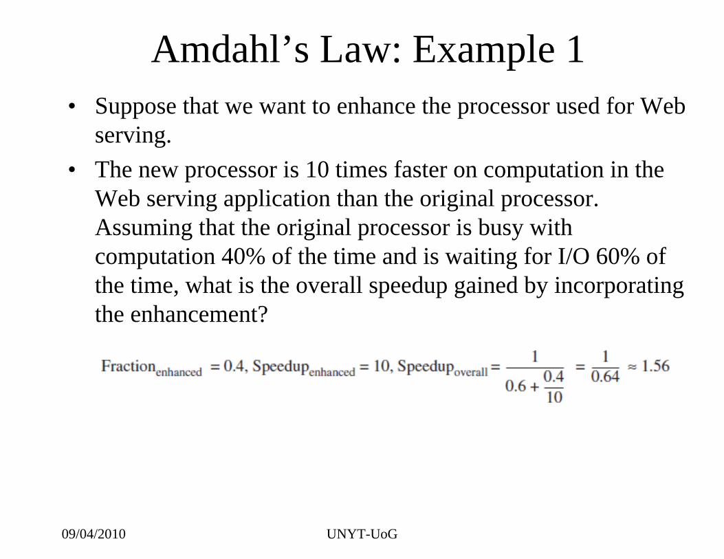
Amdahl’s Law: Example 1• Suppose that we want to enhance the processor used for Web

serving. • The new processor is 10 times faster on computation in the

Web serving application than the original processor. Assuming that the original processor is busy with computation 40% of the time and is waiting for I/O 60% of the time, what is the overall speedup gained by incorporating the enhancement?

09/04/2010 UNYT-UoG

Amdahl’s Law: Example 2• A common transformation required in graphics processors is square

root. Implementations of floating-point (FP) square root vary significantly in performance, especially among processors designed for graphics.

• Suppose FP square root (FPSQR) is responsible for 20% of the execution time of a critical graphics benchmark. – One proposal is to enhance the FPSQR hardware and speed up

this operation by a factor of 10. – The other alternative is just to try to make all FP instructions in

the graphics processor run faster by a factor of 1.6; FP instructions are responsible for half of the execution time for the application.

• The design team believes that they can make all FP instructions run 1.6 times faster with the same effort as required for the fast square root.

• Compare these two design alternatives!!!

09/04/2010 UNYT-UoG

Amdahl’s Law: Example 2• We can compare these two alternatives by

comparing the speedups:

• Improving the performance of the FP operations overall is slightly better because of the higher frequency.

09/04/2010 UNYT-UoG

The Processor Performance Equation• Essentially all computers are constructed using a clock running at

a constant rate.• These discrete time events are called ticks, clock ticks, clock

periods, clocks, cycles, or clock cycles.• Computer designers refer to the time of a clock period by its

duration (e.g., 1 ns) or by its rate, cycles per second, (e.g., 1 GHz).

• CPU time for a program can then be expressed two ways:

CPU time = CPU clock cycles for a program × Clock cycle time

Or alternatively:

09/04/2010 UNYT-UoG

Clock cycles per instruction• In addition to the number of clock cycles needed to execute

a program, we can also count the number of instructions executed — the instruction path length or instruction count (IC).

• If we know the number of clock cycles and the instruction count, we can calculate the average number of clock cycles per instruction (CPI).

• Because it is easier to work with we use CPI. • Designers sometimes also use instructions per clock (IPC),

which is the inverse of CPI.• CPI is computed as:

09/04/2010 UNYT-UoG

CPU Time• By transposing instruction count in the above formula, clock cycles can

be defined as IC × CPI. This allows us to use CPI in the execution time formula:

CPU time = Instruction count × Cycles per instruction × Clock cycle time• Expanding the first formula into the units of measurement shows how

the pieces fit together:

• As this formula demonstrates, processor performance is dependent upon three characteristics: clock cycle (or rate), clock cycles per instruction, and instruction count.

• Furthermore, CPU time is equally dependent on these three characteristics:– A 10% improvement in any one of them leads to a 10%

improvement in CPU time.

09/04/2010 UNYT-UoG

Improving CPU performance• Unfortunately, it is difficult to change one parameter in

complete isolation from others because the basic technologies involved in changing each characteristic are interdependent:– Clock cycle time — Hardware technology and

organization– CPI — Organization and instruction set architecture– Instruction count — Instruction set architecture and

compiler technology• Luckily, many potential performance improvement

techniques primarily improve one component of processor performance with small or predictable impacts on the other two.

09/04/2010 UNYT-UoG

Total CPU cycles• Sometimes it is useful in designing the processor to calculate the number

of total processor clock cycles as:

where ICi represents number of times instruction i is executed in a program and CPIi represents the average number of clocks per instruction for instruction i.

• This form can be used to express CPU time as

and overall CPI as

09/04/2010 UNYT-UoG

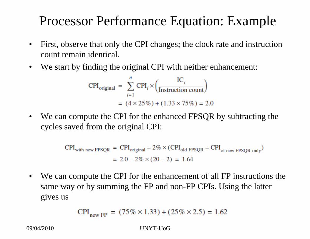
Processor Performance Equation: Example

• Consider again the example of the FPSQR.• Suppose we have made the following measurements:

– Frequency of FP operations = 25%– Average CPI of FP operations = 4.0– Average CPI of other instructions = 1.33– Frequency of FPSQR= 2%– CPI of FPSQR = 20

• Assume that the two design alternatives are to decrease the CPI of FPSQR to 2 or to decrease the average CPI of all FP operations to 2.5.

• Compare these two design alternatives using the processor performance equation.

09/04/2010 UNYT-UoG

Processor Performance Equation: Example• First, observe that only the CPI changes; the clock rate and instruction

count remain identical. • We start by finding the original CPI with neither enhancement:

• We can compute the CPI for the enhanced FPSQR by subtracting thecycles saved from the original CPI:

• We can compute the CPI for the enhancement of all FP instructions the same way or by summing the FP and non-FP CPIs. Using the latter gives us

09/04/2010 UNYT-UoG

Processor Performance Equation: Example

• Since the CPI of the overall FP enhancement is slightly lower, its performance will be marginally better.

• Specifically, the speedup for the overall FP enhancement is:

• We obtained this same speedup using Amdahl’s Law.

09/04/2010 UNYT-UoG




09/04/2010 UNYT-UoG

Performance and Price-Performance for Desktop andRack-Mountable Systems

• Although there are many benchmark suites for desktop systems, a majority of them are OS or architecture specific.

• In this section we examine the processor performance and price-performance of a variety of desktop systems using the SPEC CPU2000 integer and floating-point suites.

• SPEC CPU2000 summarizes processor performance using a geometric mean normalized to a Sun Ultra 5, with larger numbers indicating higher performance.

09/04/2010 UNYT-UoG

Systems

09/04/2010 UNYT-UoG

Comparing PerformanceThe Itanium 2–based design has the highest floating-point performance but also the highest cost, and hence has the lowest performance per thousand dollars,being off a factor of 1.1–1.6 in floating-point and 1.8–2.5 in integer performance.While the Dell based on the 3.8 GHz Intel Xeon with a 2 MB L2 cache has the high performance for CINT and second highest for CFP, it also has a much highercost than the Sun product based on the 2.4 GHz AMD Opteron with a 1 MB L2 cache, making the latter the price-performance leader for CINT and CFP.

09/04/2010 UNYT-UoG

Performance and Price-Performance forTransaction-Processing Servers

• One of the largest server markets is online transaction processing (OLTP). – The standard industry benchmark for OLTP is TPC-C, which relies on a

database system to perform queries and updates. Five factors make the performance of TPC-C particularly interesting.

• First, TPC-C is a reasonable approximation to a real OLTP application. Although this is complex and time-consuming, it makes the results reasonably indicative of real performance for OLTP.

• Second, TPC-C measures total system performance, including the hardware, the operating system, the I/O system, and the database system, making the benchmark more predictive of real performance.

• Third, the rules for running the benchmark and reporting execution time are very complete, resulting in numbers that are more comparable.

• Fourth, because of the importance of the benchmark, computer system vendors devote significant effort to making TPC-C run well.

• Fifth, vendors are required to report both performance and price-performance, enabling us to examine both.

• For TPC-C, performance is measured in transactions per minute (TPM),while price-performance is measured in dollars per TPM.

09/04/2010 UNYT-UoG

Systems

09/04/2010 UNYT-UoG

Performance and Price-performance

09/04/2010 UNYT-UoG

Performance and Price-performance• The highest-performing system is a 64-node shared-memory

multiprocessor from IBM, costing a whopping $17 million. – It is about twice as expensive and twice as fast as the

same model half its size, and almost three times faster than the third-place cluster from HP.

• The computers with the best price-performance are all uniprocessors based on Pentium 4 Xeon processors, although the L2 cache size varies.

• Notice that these systems have about three to four times better price-performance than the high-performance systems.

• Although these five computers also average 35–50 disks per processor, they only use 2.5–3 GB of DRAM per processor.

09/04/2010 UNYT-UoG




09/04/2010 UNYT-UoG

Pitfall and Fallacies• The purpose of this section, is to explain some commonly

held misbeliefs or misconceptions that you should avoid. • We call such misbeliefs fallacies.• When discussing a fallacy, we try to give a counterexample.• We also discuss pitfalls — easily made mistakes. • Often pitfalls are generalizations of principles that are true in

a limited context. • The purpose of these sections is to help to avoid making

these errors in computers design.

09/04/2010 UNYT-UoG

Pitfall: Falling prey to Amdahl’s Law

• Virtually every practicing computer architect knows Amdahl’s Law.

• Despite this, we almost all occasionally expend tremendous effort optimizing some feature before we measure its usage.

• Only when the overall speedup is disappointing do we recall that we should have measured first before we spent so much effort enhancing it!

09/04/2010 UNYT-UoG

Pitfall: A single point of failure.• The calculations of reliability improvement using Amdahl’s

Law show that dependability is no stronger than the weakest link in a chain.

• No matter how much more dependable we make the power supplies, as we did in our example, the single fan will limit the reliability of the disk subsystem.

• This Amdahl’s Law observation led to a rule of thumb for fault-tolerant systems to make sure that every component was redundant so that no single component failure could bring down the whole system.

09/04/2010 UNYT-UoG

Fallacy: The cost of the processor dominates the cost of the system.

• Computer science is processor centric, perhaps because processors seem more intellectually interesting than memories or disks and perhaps because algorithms are traditionally measured in number of processor operations.

• This fascination leads us to think that processor utilization isthe most important figure of merit.

• Indeed, the high-performance computing community often evaluates algorithms and architectures by what fraction of peak processor performance is achieved.

• This would make sense if most of the cost were in the processors.– This is not true!

09/04/2010 UNYT-UoG

Breakdown of costs

09/04/2010 UNYT-UoG

Fallacy: Benchmarks remain valid indefinitely

• Several factors influence the usefulness of a benchmark as a predictor of real performance, and some change over time.

• A big factor influencing the usefulness of a benchmark is its ability to resist “cracking,” also known as “benchmark engineering” or “benchmarksmanship.”

• Once a benchmark becomes standardized and popular, there is tremendous pressure to improve performance by targeted optimizations or by aggressive interpretation of the rules for running the benchmark.

• Small kernels or programs that spend their time in a very small number of lines of code are particularly vulnerable.

• Example: next slide

09/04/2010 UNYT-UoG

Benchmarksmanship• For example, despite the best intentions, the initial SPEC89

benchmark suite included a small kernel, called matrix300, which consisted of eight different 300 × 300 matrix multiplications.

• In this kernel, 99% of the execution time was in a single line (see SPEC [1989]).

• When an IBM compiler optimized this inner loop (using an idea called blocking), performance improved by a factor of 9 over a prior version of the compiler!

• This benchmark tested compiler tuning and was not, of course, a good indication of overall performance, nor of the typical value of this particular optimization.

09/04/2010 UNYT-UoG

Fallacy: The rated mean time to failure of disks is 1,200,000 hours or almost 140 years, so disks practically never fail.

• The current marketing practices of disk manufacturers can mislead users.

• How is such an MTTF calculated? Early in the process, manufacturers will put thousands of disks in a room, run them for a few months, and count the number that fail.

• They compute MTTF as the total number of hours that the disks worked cumulatively divided by the number that failed.

• One problem is that this number far exceeds the lifetime of a disk, which is commonly assumed to be 5 years or 43,800 hours.

• For this large MTTF to make some sense, disk manufacturers arguethat the model corresponds to a user who buys a disk, and then keeps replacing the disk every 5 years — the planned lifetime of the disk. – The claim is that if many customers (and their great grandchildren) did

this for the next century, on average they would replace a disk 27 times before a failure, or about 140 years.

09/04/2010 UNYT-UoG


• A more useful measure would be percentage of disks that fail.

• Assume 1000 disks with a 1,000,000-hour MTTF and that the disks are used 24 hours a day.

• If you replaced failed disks with a new one having the same reliability characteristics, the number that would fail in a year (8760 hours) is:

• Stated alternatively, 0.9% would fail per year, or 4.4% over a 5-year lifetime.

09/04/2010 UNYT-UoG


• Moreover, high numbers are quoted assuming limited ranges of temperature and vibration; if they are exceeded, then all bets are off.

• A recent survey of disk drives in real environments [Gray and van Ingen 2005] claims about 3–6% of SCSI drives fail per year, or an MTTF of about 150,000–300,000 hours, and about 3–7% of ATA drives fail per year, or an MTTF of about 125,000–300,000 hours.

• The quoted MTTF of ATA disks is usually 500,000–600,000 hours.

• Hence, according to this report, real-world MTTF is about 2–4 times worse than manufacturer’s MTTF for ATA disks and 4–8 times worse for SCSI disks.

09/04/2010 UNYT-UoG

Fallacy: Peak performance tracks observed performance

• The only universally true definition of peak performance is “the performance level a computer is guaranteed not to exceed.”

• Next slide shows the percentage of peak performance for four programs on four multiprocessors.

• It varies from 5% to 58%. • Since the gap is so large and can vary significantly by

benchmark, peak performance is not generally useful in predicting observed performance.

09/04/2010 UNYT-UoG

Fallacy: Peak performance tracks observed performance

09/04/2010 UNYT-UoG

Pitfall: Fault detection can lower availability• This apparently ironic pitfall is because computer hardware has a

fair amount of state that may not always be critical to proper operation.

• In processors that try to aggressively exploit instruction-level parallelism, not all the operations are needed for correct execution of the program. Mukherjee et al. [2003] found that less than 30% of the operations were potentially on the critical path for the SPEC2000 benchmarks running on an Itanium 2.

• The same observation is true about programs. • If a register is “dead” in a program — that is, the program will

write it before it is read again — then errors do not matter. If you were to crash the program upon detection of a transient fault in a dead register, it would lower availability unnecessarily.

• The pitfall is in detecting faults without providing a mechanism to correct them.

09/04/2010 UNYT-UoG

End of Lecture 1• Readings

– Book: Chapter 1

advanced topics in computer architecture - marenglen … · 09/04/2010 unyt-uog advanced topics in...

Documents