advanced stochastic analysis program for offshore …
TRANSCRIPT
ADVANCED STOCHASTIC ANALYSIS PROGRAMFOR OFFSHORE STRUCTURES
Theoretical outline and the User's Manual ofSAPOS
TU DelftDeIft University of Technology
by
Dr. H. KARADENIZ
Report No.: 25.2.89.1.11
August, 1989
FacUlty of civil EngineeringDMalonof Mechanics and StructuresSection of pplIed Mechanics
TECHNISCHE UNIVER$iiitLaboratolium voor
ScheepshydromechaArchlef
MekeiWeg 2,2628 CD DeiftTol. 015.788813. Faz 015.781858
- SAPOS -
CONTENTS
1- INTRODUCTION 1
2- SPECTRAL ANALYSIS 32.1 - General Concept and Traditional Modal Analysis Technique 3
2.2 - Modified Modal Analysis Technique 62.3 - Transfer functions of Wave Forces 72.4 - Direct Formulation of Stress Transfer-function 92.5 - Calculation of stress statistical characteristics 11
3- STOCHASTIC FATIGUE DAMAGE CALCULATION 13
4- UNCERTAINTY MODELLING AND RELIABILITY CALCULATION 164.1 - Uncertainties in the Fatigue Damage 16
4.1.1 - Structural Category 16Stiffness matrix 16Mass matrix 16Damping matrix 17
4.1.2 - Loading and Environmental Category 18Wave loading 18Modelling, of random wave environment 18
4.1.3 - Fatigue Category 20Stress Concentration Factors 21S-N model 21
c.) Damage Correction Factor 214) Reference Damage . . 22
4.2 - Limit State Function and The Reliability Calculation 22
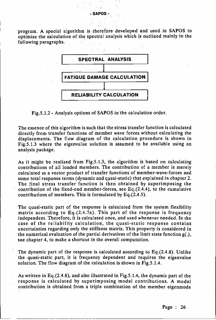
5- PROGRAM OUTLINE AND GENERAL DESCRIPTION 255.1 - Outline of the Program 255.2 - General Description . 29
6- PROGRAM INPUTS . . 326.1 - Indirect Inputs . 32
6.1.1 - INCidences of submerged members 326.1.2 - BOOkkeeping degrees of freedom of submerged joints 33&1.3 -. COOrdinates of submerged joints 346.1.4 - iMSplacements (EIGENMode vectors) of submerged joints 3561.5 MODal (GENeralized) masses 366.1.6 - NATural frequencies (EIGENVa1ues). 366.1.7 - PROpertIes of submerged members 376.1.8 - FLExibility matrix (stored columnwise from diagonal 'terms) 38
'6.2 - Direct Inputs 406.2..1 - DAMping ratios 406.2.2 - MATerial constants 406.2.3 - LOAding properties .. 41
Page : I

- SAPOS -
6.2.4 - WAVe properties F - i directional sea 41L[MULti-] J
6.2.5 - MAIn wave direction r 46.2,6 - GAUss points for frequency integration 43
[sPEctral ] [STAtic 1.627- FATigue analysis ID'am1c I contribution 43
LRELiabiUy J LSTAtic + DYNamicj
[FORCES i6.2.8 - LIST STRESses for the sea state h (and t) 46
[SPECTral moments J
6.2.9 - SEA properties [Jswap]] spectrum, SCA (DIA) 47
6.2.10-UNLoaded members 516.2.11 - STRess (FORce) locations 516.2.12 - LIFe (SERvice) time 526.2.13- ITERation number of the reliability analysis 536.2.14 - DESign variables 53
PROGRAM OUTPUTS 567.1 - Standard Outputs 567.2 User contr011ed Outputs 57
DEMONSTRATION - 58
REFERENCES 71
Page : II

- SAPOS -
ADVANCED STOCHASTIC ANALYSIS PROGRAMFOR OFFSHORE STRUCTURES
Theoretical outline and the User's Manual ofSAPOS
1- INTRODUCTION
This report is intended primarily to describe an update version of the computerprogram, SAPOS [1], as being a user's manual, and secondarily to outline thetheoretical background of the update. SAPOS stands for Stochastic Analysisprogram for Offshore Structures, which is a sophisticated computation-tool forthe spectral, fatigue and fatigue-reliability analyses of offshore structures.Although it is designed for practical applications, it can also be used foreducational .and research purposes., as well as for checking results of otherprogrammes. It accommodates advanced analysis methods tO put them intopractice, giving more confidence in the computation and reliability of results.SAPOS is a talented software for stochastic analysis of offshore structures, whichhas a trend to meet requirements of modern design philosophy. This updateutilizes recent algorithmic developments and improved analysis methodsproviding a better performance and more flexibility in the application. Newfeatures of the program are summarized in the following.
Effect of marine growths on the wave force calculation.JONSWAP sea spectrum as additional to Pierson-Moskowitz (P.M.) seaspectrum.Two parameters modelling of the sea spectrum as Hs (significant wave height)and Tz (mean zero crossing period of waves) with scatter diagram for thelong-term distribution of the sea state.Modification of the modal analysis technique to include the staticcontribution of the response.Con.trbution of the fixed end member forces to the stress calculation. This isdue to the distributed nature of the wave force according to Morison'sequation.Allowing for an endurance in the S-N fatigue model.An efficient modelling of uncertainty contents of fatigue damage in the caseof reliability assessment to reduce the cOmputation time.
Since SAPOS is arranged in a flexible and independent form it can be easilyimplemented into, or run with, an existing structural analysis package. Further, itoffers a very friendly and simple usage of inputs and clarity of utputs as will be
Page 1
- SAPOS -
explained later in the report. Besides its sophisticatiOn it is, however, subjectedto the following restrictions for the time being.
It runs with an analysis package. Thus, it is not completely independent in itsintegrity.Since it has no graphical facilities, direct graphical outputs are not possibleOnly wave forces are considered. Thus, wave-current interactions and otherphenomenal forces are not iÍiludéd.Structure-water interactions are not yet included.A code checking, is not implemented.Only bottom supported structures can be analyzed.FoundatiOn-structure interactions are not allowed, thus, the underlyingfoundation can be represented simply by massless springs.Contribution of shear deformations is not included in the stress analysis
As indicated above, three calculation items can be distinguished in SAPOS,which are spectral analysis, fatigue damage calculation and reliabilityassessment These items will be outlined first in next chapters and then theprogram usage will be presented later in detail.
Page : 2

2- SPECTRAL ANALYSIS
2.1- General Concept and Traditional Modal Analysis Technique
In offshore structural engineering, calculation of fatigue damage and finding asafety margin against a probable fatigue failure are of great interest to designers,to insuring and owning companies Calculation of the fatigue damage in a randomenvironment, such as in offshore, is a difficult subject and requires a stochastictreatment. Formulation of a stochastic fatigue damage can be obtained in termsof spectral moments of the stress process [2] in a structural member, which arecalculated by means of a spectral analysis procedure. It i.s meant from the spóctralanalysis that spectral values of the stress process are to be calculated. In SAPOSsuch an analysis is carried out by using the concept of transfer functions of linearsystems in which it is assumed that there are linear relations between inputs andoutputs. An overall calculation scheme of the stress spectrum is shown inFig.2.1.1.
WAVE ENVIRONMENT
STRUCTURE
¿STRUCTURAL
TRANSFERFUNCTION
- SAPOS -
w
THEORETICALTREATMENT
WAVEFORCE
TRANSFERFUNCTION
ySTRESS
TRANSFERFUNCTION
WAVERECORDS
VSEA
SPECTRUM
STRESSSPECTRUM
Fig.2.i.1 - Flow diagram of the calculation of a stress spectrum.
Page : 3

STRUCTURALTRANSFERFUNCTION
- SAPOS -
Fig.2.1.1 gives an implication of the procedure using the cOncept of transferfunctions. It is described as in the following.
Based on wave records from the wave environment, spectrum of the waveelevation (Sea spectrum) is determined This is usually known in a functionalform, and it constitutes the input spectrum of the analysis.From the theoretical point of view, using the linear wave theory, wave forcetransfer functions are calculated. Theseare dependent on the structuralconfiguration.On the other hand, some structural transfer functions are calculated as beingindependent of wave environment and thus, of wave forces.The stress transfer function is calculated by a suitable combination of thestructural and wave force transfer functions. This is shown in Fig.2.1.2, whenusing the traditjonal calculation procedure.The stress spectrum is calculated from the product of the stress transferfunction and the sea spectrum as indicated in ig.2.1.1.
WAVE FORCETRANSFERFUNCTION
LDISPLACEMENT
TRANSFERFUNCTION
Fig.2.1.2- Calculation of stress transfer functions using the traditional procedure
As it can be realized from above, a great deal of efforts are spent on thecalculation of the stress transfer function which constitutes the hearth of thespectral analysis. In thIs calculation, a special care needs to be given to a correctdetermination of structural tranSfer functions since they may affect thecalculation dramatically These functions can be derived directly from the overalldynamic equilibrium equation of the system [3] written as in the matrix nOtation,
[K] {U} + [C] {Ú} + [M] {Ü} = {F(t)} (2.1.1)
Page : 4
4STRESS
TRANSFERFUNCTION
in which, [K], [C] and [M] are respectively the overall stiffness, damping and massmatrices, {U} and {F(t)} are respectively the overall displacement and appliedforce vectors, a dot (.) denotes a time derivative. Taking the Fourier transform ofboth sides of Eq.(2.1.l), the frequency-domain equation can be written as,
([K] + iw[C] - w2 [M]) {U(w)} = {F(w)} (2.1.2)
where i=V-1, and w denotes the angular frequency. From Eq.(2 1.2) thestructural transfer functions can be stated in the matrix notation as,,
[HUF(w)] ([K] +iw[C] -
Then the displacement vector will be written from Eq.(2.1.2) as,,
{U(w)} = [HUF(w)] {F(w)} (2.1.4)
Here it is worth noting that E4.(2.1.3) is the exact form of the structural transferfunctions. As it might be realized, their evaluations take excessivecomputation-times Therefore, using Eq (2 1 3) is not suitable in practicalapplications. Instead, an approximate formulation is widely used in practice,which is obtained by employiñg the well known modal analysis technique leadingto,
[HUF(w)]
i
hr(CV) {cIr} {(br}' '(2.1.5)
In this statement, q is the total number of natural modes considered, {r}denotes an eigenmode vector,, the superscript (T) indicates a matrix transpositionand hr(w) is a frequency fünction corresponding to 'the natural mode r. Thisfunction is termed here as a modal transfer function and defined by,
i W
kr (Wr2- w2) +2irWrW
- SAPOS -
(2.1.3)
(2.1.6)
where Wr, r are respectively the natural frequency and the damping ratio to thecritical, kr is the generalized stiffness.
This traditional analysis technique was used in the previous version of SAPOS. Aconcept of Spectral Participation Factors (SPF) [4], which is based on thistechnique, was introduced to ease the analysis. Although it was elaborately usedin SAPOS the traditional technique has been known to be inadequate to producesatisfactory results in the stress analysis [5]. Satisfactoty results can only beobtained if a large number of natural modes are included in the analysis in
Page :
h (w)=

- SAPOS -
general. However, it may also depend on the structural cOnfiguration. For highlysensitive structures to dynamic excitations few natural modes may suffice toproduce good results whereas for insensitive structures good results cannot beachieved by considering only few modes. In such a case, the quasi-staticcontribution of the response becomes very important. Even it dominates thewhole response behaviour when the fundamental natural frequency of thestructure is far from the excitation frequency of the forcing phenomenon.Therefore, in this case, it cannot be truncated by using the traditional modalanalysis technique unless a large number of natural modes are included in theanalysis. This latter option is obviously computationally-awkward andunpractical. In order to eliminate this unpleasant situation and to improve theperformance of the modal analysis technique, an alternative procedure, which isused in the update version of SAPOS, is presented below.
2.2- Modified Modal Analysis Technique
As outlined above, the traditional modal analysis technique fails to produce acomplete structural response. The quasi-static part of the response is notsufficiently taken into account in the analysis. Alternatively, a pure quasi-staticanalysis does not include the dynamic contribution. It seems however that ananalysis technique which takes into account both the quasi-static and dynamiccontributions, which is also computationally practical, is likely the most Suitableand desirable in the calculation of spectral response stresses. Starting from thispoint of view of thinking, a structural transfer function matrix can be defined as,
[HUF(w)] [K]' +ar(w) {} {r}T (2.2.1)
where the first term on the right hand side corresponds to the quasi-staticsolution and the second one is included to represent the dynamic contribution. InEq.(2.2.1) the parameter ar(w) is a complex frequency function which determinesthe participation of the natural mode r. This parameter is obtained [6] to be,
ar(w) hr(W) - (2.2.2)
where hr(w) is defined by Eq.(2.1.6) and kr is the generalized stiffness for themode r
This modified modal analysis technique is implemented into SAPOS. It reducescomputation-time considerably and produces accurate results. Additionally, itprovides flexibility in usage as probably to apply a pure quasi-static analysis orthe traditional modal analysis technique. These options are also available inSAPOS, and can be activated by user's command. An efficient calculationalgorithm is developed, to manipulate this advanced technique in the program.The algorithm is based on eliminating the displacement field from thedetermination of stress transfer functions, thus direct relations between applied
Page : 6

- SAPOS -
forces and resulting stresses are constituted. This is a remarkable achievementthat prevents excessive calculations in the spectral analysis. This subjèct will beexplained in section 2.4. First, transfer functions of wave forces are presented inthe following section.
2.3- Transfer functions of Wave Forces
Wave forces acting on offshore structural members are calculated from Morison'sequation. These forces are distributed along member length.s and being normalto member axes as shown in Fig.2.3.1.
J4PLÀ4w.
Wave direCtbO,X
t,
Normal watervelocity
Morison 's
p = CD k
Member axis
equationw +
a) structural system under wave b) wave loading on a member
Fig.2.3.1 A schematic offshore structure and wave loading.
Morisón's equation is Writtén in the time domain as,
p = CD Iwl. w + M' (2.3.1)
where w and * are respectively water velocity and acceleration being normal tothe member, Ci pCdDh/ 2 and CM =JrpcmDh2/ 4 in which p is the mass densityof water, Cd and Cm are respectively the drag and inertia force coefficients, Dhdenotes an increased member diameter due to marine growth. As it is seen fromEq (2 3 1) the drag force term in the Morison's equation is non- linear withrespect to the water velocity w. In order to employ the concept of transferfunctions, this term needs to be linearized somehow In SAPOS, a linearizationtechnique is used assuming that the linearized and non-linear forces produce thesame variance. The linearized Morison's equation can be written in vectorialnotation as,
Page : 7

- SAPOS -
{p} = f(0) CD Ou {w} + CM {''} (2.3.2)
where f(0) is a function of wave direction angle, see Fig.2.3.1 (a), and °u is thestandard deviation of horizontal water velocity in the wave direction Using thelinear wave theOry and Eq.(2.3.2) the wave force vector can be written in thefrequency domain [4] as,
{p(w)} = {H,7(w)} (w) (2.3.3)
where ij(w) denotes water elevation, which is considered as the input of theanalysis, and {Hp,1(w)} denotes transfer function vector of the wave forceaccording to the Morison's equation. This vector can be stated as,
{Hp,7(w)} = (f(0) CD au + i(I) CM) {Hw,1(w)} (2.3.4)
in which {H,7(w)} denotes transfer function vector between the normal watervelocity and the watet elevation. The transfer functiOn vector of the wave force,given by Eq.(2.3.4), is written per unit member length. Its distribution isexponential in vertical direction and harmonic in horizontal direction. Usingprinciples of external work, transfer functions of equivalent wave forces atmember ends will be calculated, assuming that cubic polynomial fui ctions areused to represent member deformations. These transfer functions can. be writtenin vectorial notation as, e.g. fr member i,
{HpL(w)}i tN]i {H(w)} dx (2.3.5)
where [N] denotes shape function matrix ofmember deformations, l denotes themember length and x denotes a variable along the member axis. The subscript (L)in above statement indicates local coordinates. For the assemblage this vectorwill be transformed to the global coordinates, see Fig.2.3.2 for local and globalcoordinates.
z
X
a) Member local coordinates b) Member global coordinates
Fig.2.3.2- Member coordinate systems
Page : 8
- SAPOS -
The transformation is wr1tten as,
{HF,7(w)}i = rT]iT{HFL(w)}i (2.3.6)
where {HF,7(w)}i is the transfer function vector of consistent member forces inglobal coordinates and [T]i is a transformation matrix between member degreesof freedom in two còordinate systems. The subscript i denOtes a member. Havingcalculated transfer functions of member forces, an assembly process will becarried out to obtain transfer functions Of overall wave forces. This process isformulated as,
{HF)} =: {HF(w)}i (2.3.7)
where [B] is a matrix which determines locations of member degrees of freedomin the overall system (its elements are either i or O), n denotes total number ofloaded members. This corresponds to the traditional analysis and may be timeconsuming in the dynamic stress calculation which is largely applied in thisreport. An alternative procedure, which seems to be more efficient andpromising, is used in SAPOS Basic formulations of this attractive procedure ispresented in the following section.
2.4' Direct Formulation of Stress Transfer-function
When the straightforward procedure is applied, the usual way of determining astress transfer fúnction is to calculate displacement transfer-functions first, andthen, transfer functions of member internal forces. In the alternative procedure,it is so formulated that the stress transfer function can be obtained directly fromthose of applied forces This is achieved by eliminating displacements from thecalculation of the stress. The formulation of this powerful procedure is actuallyderived from the traditional procedure, and therefore, it is presented first.
Similar to Eq.(2.1.4), transfer functions of system displacements can be writtenin matrix notation as,
{Hu,7(w)} [HuF(w)] {HF7J(w)} (2.4.1)
in which [HuF(w)] and {HF,(a)} are calculated respectively from Eqs.(2.2.1)and (2.3.7). Transfer functions of member displacements will now be extractedfrom Eq.(24.1). This extraction is formulated as, e.g. for a stress member j,
{Hu,7(w)}j [BlT {Hu,7(w)} (2.4.2)
Page : 9
-SAPOS-
where [B] is the same matrix as in Eq.(2.3.7.), but this time it is for the stressmember j. The vector given by Eq.(2.4.2) will be transformed to member localcoordinates first, and then, transfer-functions óf member internal forces will becalculated from,
{Ho,7(w)} = [KL]j {HuL(w)}j - {HFL,7(w)}j (2.4.3)
where the subscript L denotes local coordinates, {Ho(w)}j is the vector oftransfer functions òf the member internal forces, [KL]j is the member stiffnessmatrix, {HUL(w)}j is the transfer function vector of member displacements inlocal coordinates, and {HFL,7(w)}j is calculated from Eq.(2.3.5), for the stressmember j, which represents the contribution of fixed-end member-forces.Transfer function of a stress at a given location can now be calculated using thelinear relation between internal forces and the stress. This is formulated as,
H7(co)J {L}j' {H(w)} (2.4.4)
where {L} is a vector containing member properties (cross- sectional area andinertia moments), and H,7(w) is the stress transfer function we would like tocalculate.
The alternative procedure is formulated by introducing transfer functions ofdisplacements, given by Eqs.(2.4.1) and (2.4.2), into Eq.(2.4.3), and by makinguse of Eqs.(2.3.7) and (2.2.1). In this procedure, contributions of transferfunctions of member wave forces to the stress transfer function are calculatedfirst. Then, the total stress transfer function is obtained by superimposingindividual contributions of member forces, which is written as,
Hs(w)j {Z(w)} {HFL)}i - {L}jT{HFL(w)}j (4.5)
where n denotes the number of loaded members. In Eq.(2.4.5), the vector,{Z(w)}, determines the participation of a loaded member in thestress transferfunction, the vectors {HFL,7(w)}i and {HFL,7(w)}j are respectively transferfunction vectors of consistent forces of a loaded member i and the stress memberj. These vectors will be calculated from Eq.(2.3.5). The participation vector,{Z(w)}, is obtained to be,
{Z(w)} = + {V(w)}ji (2.4.6)
where the vectors {U}i and {V(w)} represent respectively the quasi-static anddynamic parts of the response. As it might be realized from Eq.(2.4.6) thequasi-static part is a frequency independent vector unlike the dynamic part whichis a function of the frequency, but independent of the wave loading. The quasi-static part is formulated as,
Page 10

-SAPOS.
[T]i [A]Ji[T]jT [KL]j {L} (2.4.7a)
where the matrix [A]ï determines the participation of a loaded member inquasi-static displacements of the stress member j This matrix is defined as,
[BIIT [K]4 [B]j (2.4.7b)
in which [K]' is the system flexibility matrix. The dynamic part in Eq.(2.4.6) issimply calculated from,
q
{V(w)} =) (ar(W) sjr) {bLr}i (2.4.8)
r=1where Sjr is a modal stress corresponding to the eigenmode r, ar(w) is as definedby Eq.(2.2.2), and {Lr}i is the eigenmode vector of a loaded member in localcoordinates.
Calculation of the quasi-static part of the response from Eq.(2.4.7) looks likecomplicated. As a matter of fact, it is very simple and needs to be calculated oncefor all frequency variations Although the calculation of the matrix [A]JL from
E.(2.4.7b) seems to require matrix multiplications, in fàct, it is a matter ofextraction from the system flexibility matrix.
2.5- Calculation of stress statistical characteùistics
As it will be explained in the next chapter, a cumulative fatigue damage isformulated depén4ently on some stress statistical characteristics which arecalculated in terms of spectral moments of the stress. In this calculation, anarrow-band stationary Gaussian process is assumed for the stress variation.Stress spectral moments are calculated from the frequency integration,
00
mn Jwn' Sss(co) dw (2.5.1)
where n shows the degree of the moment and Sss(w) is the stress spectrum. Inpractice,, the frequently used. spectral moments (zero, second and fourth degrees)are obtained by using n 0, 2 and 4. The stress spectrum is calculated in termsof the stress transfer function and a sea spectrum as written by, for a stressmember j,
S(w) = Hs.*,l(w)j H,7(w) S,7(w) (2.5.2)
where H,(w) is the stress transfer function calculated from Eq.(2.4.5), the (*)denotes a complex conjugate, and S,7(w) is an assumed sea spectrum. If,
Page: 11.
SAPOS
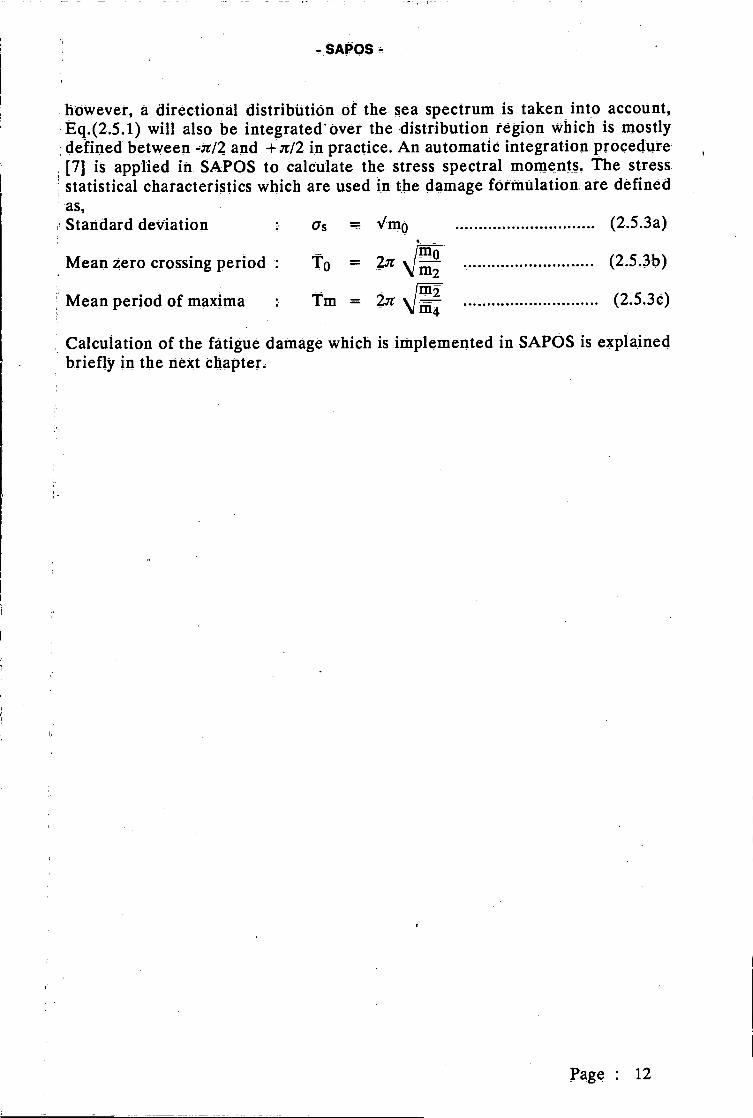
however, a directional distribütiön of the sea spectrum is taken into account,Eq (2 5 1) will also be integrated over the distribution region which is mostlydefined between -r/2 and +r/2 in practice An automatic integration procedure[7] is applied in SAPOS to calculate the stress spectral moments The stressstatistical characteristics which are used in. the damage förmulation. are definedas,Standard deviation (m0 (2.5.3a)
Mean zero crossing period : T0 = 2r \1iii. (2.5.3b)
Mean period of maxima Ïm = 2.ir (2.5.3c)
Calculation of the ftigue damage which is implemented in SAPOS is explainedbriefly in the next chapter
Page : 12
SAPOS -
3- STOCHASTIC FATIGUE DAMAGE CALCULATION
Calculation of the stochastic fatigue damage is carried ou in SAPOS assumingthat,
an experimentally determined S-N fatigue model is known,the stress process is a narrow-band stationary Gaussian,the well known Palmgren-Miner's rule is applied.
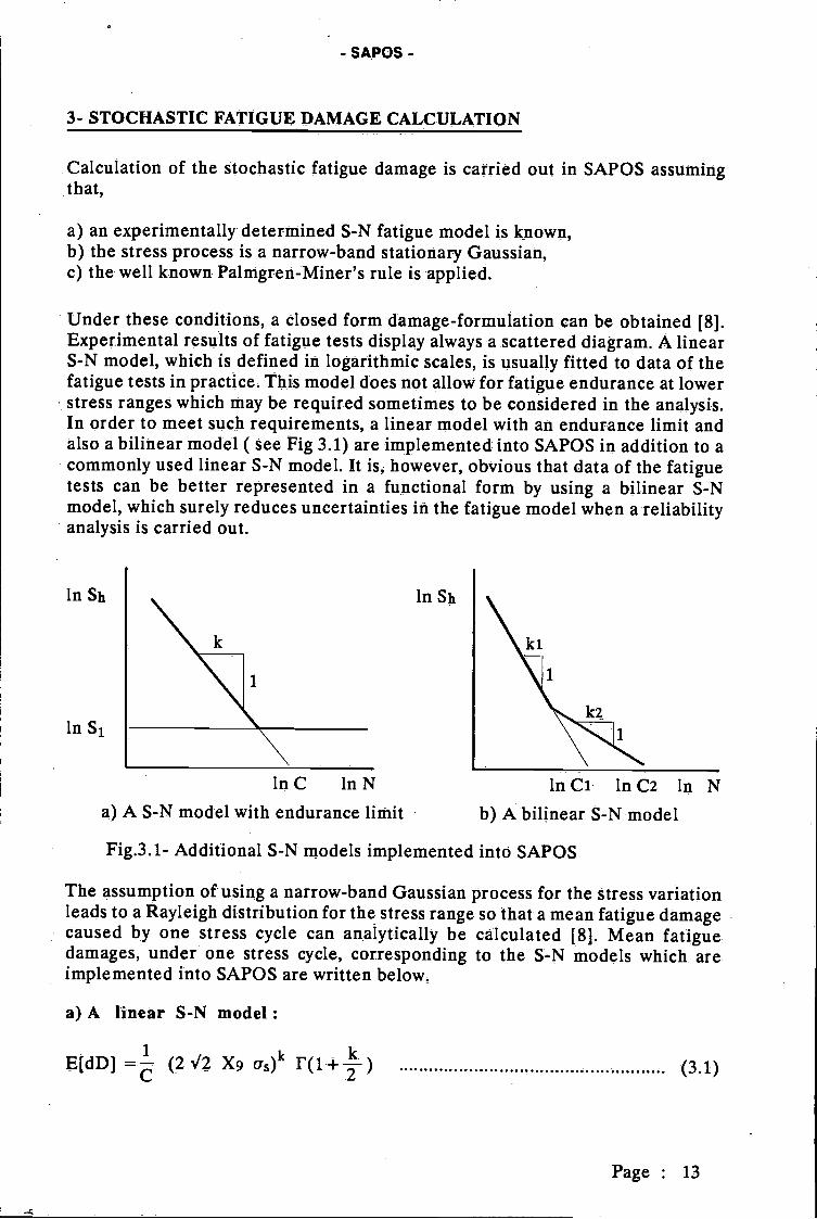
Under these conditions, a closed form damage-formulation can be obtained [8].Experimental results of fatigue tests display always a scattered diagram A linearS-N model, which is defined in logarithmic scales, is usually fitted to data of thefatigue tests in practice. This model dòes not allow for fàtigue endurance at lowerstress ranges which may be required sometimes to be considered in the analysis.In order to meet such requirements, a linear model with an endurance limit andalso a bilinear model ( See Fig 3.1) are implemented into SAPOS in addition to acommonly used linear S-N model. It is, however, obvious that data of the fatiguetests can be better represented in a functional form by using a bilinear S-Nmodel, which surely reduces uncertainties in the fatigue model when a reliabilityanalysis is carried out.
in Sb
in S
ln Sb
inC inN mCi lnC2 in Na) A S-N model With endurance limit b) A bilinear S-N model
Fig.3.1- Additional S-N models implemented intò SAPOS
The assumption of using a narrow-band Gaussian process for the Stress variationleads to a Rayleigh distribution for the stress range so that a mean fatigue damagecaused by one stress cycle can analytically be calculated [8]. Mean fatiguedamages, under one stress cycle, corresponding to the S-N models which areimplemented into SAPOS are written below,
a) A linear S-N model:
E[dD] = (2v'2 X9 us)k r(1±--) (3.1)
Page : 13

where C and k are the fatigue parameters, X9 is a random variable with u(X9) = irepresenting uncertainties in the stress concentration factors (SCF) of thenormal force and bending moments, as is the standard deviation of the stress at ahot- spot, and r(.) denotes the Gamma function.
b) A linear S-N model With an endurance limit:
E[dD]=c
(2V2X9Os)kF(l+ y)
where T(.,.) denotes the incomplete Gamma function [9], and the parameter y isdefined as,
i S Z
X9U
in which Si is the endurance limit shown as in Fig.3.1.a.
e) A bilinear S-N model:
i k1 kl-k2. k2 k2E[dD] = - (2V2X9as)kl(T(1±_,y)+y 2 (I'(l+ --)-F(1+ ,y))) (3.3a)
C1 2 2
where Ci and ki, C2 and k2 are the parameters of the bilinear S-N model, seeFig.3.lb. The parameter, y, is defined as,
C2 2/k2-kP -2y (-) ' (2v'2 X9 as) (3.3b)Ci
The damage caused by one stress cycle will be accumulated during a sea state andin a long-term period The cumulative damage is simply calculated bysuperimposing the damages of one cycle in an assumed period of time Since seastates in the long-term are usually described to be probabilistic, the mean of thecumulative damage in. the long-term can be stated as,
Dtot T JJ E[dD] fHs,Tz(h,t) dh dt (3.4)
where T is an assumed life-time, To is the mean zero-crossing period calculatedfrom Eq.(2.5.3), and fHs,Tz(h,t) is a joint probability density function of H andT which represent the sea state in the long-term If, however, the sea state isrepresented by H5 only, the density function fHs,Tz(h,t) will be replaced by themarginal density function of H and this will be denoted by, fHs(h) Theparameter, ..%, in Eq.(3.4) is a damage correctiOn factor due to the fact that thedamage is formulated by using a narrow-band stress process But, in practice, thestress process iS usually non narrow-banded and displays a bimódal spectral
Page : 14
- SAPOS -
(3.2a)
(3. 2b)

- SAPOS -
shape so that the damage due to the ñarrow-band stress process is corrected bythe parameter, . This parameter is a function of the spectral bandwidth of thestress process as well as slope(s) of the S-N fatigue model used.
As it will be. explained later, a cOntinuous joint density function of H and Tzwhich is based on a provided scatter diagram. is also implçmented into SAPOS, inaddition to using a discrete scatter diagram If the sea state is represented by Hs,in the long-term, a three parameters Weibull and a log-normal probabilityfunctions are provided in .the program fr the marginal distribution of H. If,however, multiple main-wave directions are to be considered, Eq (3 4) will alsobe integrated over O23r, assuming that the main-wave direction is uniformlydistributed in O-2x..
n the above equatiOns of the àtigue damage there are some inevitableuncertainties that must be taken into account when a reliability analysis is carriedout These uncertainties and the reliability calculation, which are treated inSAPOS, are explained in the following chapter.
Page : 15

- SAPOS -
4- UNCERTAINTY MODELLING AND RELIABILITY CALCULATION
4.1- Uncertainties in the Fatigue Damage
Uncertainties in the cumulative fatigue damage presented by Eq.(3.4), may be.classified in three categories as:
structural,loading and environméntal,fatigue related.
These uncertainty groups are. discussed below separately.
4.1.1- Structural Category
Uncertainties reflected in the system stiffness, mass and damping matrices areconsidered in this category as explained in the following.
Stiffness matrix : Member thicknesses and foundation parameters may beconsidered as major uncertainty origins. The total stiffness matrix can be statedin the uncertainty space as,
Xk 4u([K]) = Xt 4u([Kt]) + Xg 4u([Kg]) (4.1.1.1)
where Xk, Xt and Xg are respectively uncertainty parameters in the system,structural and foundation stiffness matrices, p([K]), 4u([Kt]) and 1u([Kg]) are thecorresponding mean matrices. As it may be realized from Eq.(4.1.1.1) the meanvalues of the uncertainty parameters are all equal to 1. In SAPOS, Xk is used torepresent the total uncertainty related to the system stiffness matrix. Asmentioned, its mean value equals 1. Its variance can be estimated from,
Xk = Xt (r + Xg (-)r (4.1.1.2)
where k, kt and kg are the generalized stiffnesses calculated respectively by usingthe matrices 1u([K]), 4u([Kt]) and 4u([Kg]), the subscript r denotes an eigenmodeIt is likely that Eq.(4.1.1.2) produces different values of Xk for differenteigenmodes in which case an average value of the variance can be used.
Mass matrix : Added masses due to structure-water interactions, the mass ofthe deck and structural masses due to member thicknesses are considered to besubstantial uncertainty origins. Similar to the stiffness matrix, the total massmatrix can be stated in the uncertainty space as,
Xm u([M]) = .Xt /«[Mt]) + Xa ¿u([Ma]) + Xd u([Md]) + [M] (4.1.1.3)
Page : 16

SAPOS -
where Xm, Xt (same as in thé stiffness matrix), Xa, and Xd are respectivelyuncertainty parameters of the system, structural, added, and deck mass matrices,u([M]), u([Mt]), i«[Ma]) and u([Md]) are the corresponding mean matrices. Thematrix [Mw] in Eq.(4.1.Í.3) is a deterministic matrix due to water included inmembers. Mean values of these uncertainty parameters are all eqúal to 1. Theparameter Xm is used in SAPOS to represent all uncertainties related to thesystem mass matrix. Given statistical characteristics of Xt, Xa and Xd, thevariance of Xm can be calculated from,
Xrn = X ( )r + Xa ( -)r + Xd ( -)r +( (4.1.1.4)
where m, mt, ma, m and mw are the mean generalized masses. Since thethickness parameter,, Xt, is defined in both the stiffness and mass matrices incommon, Xk and Xm Will be correlated variables to some degree. Thé correlationcoefficient can be obtained by using Eqs.(4.1.1.2) and (4.1.1.4). Then, these twodependent variables Will be made independent by an orthogonal transformation[4]. The independent variables, which are denoted by Xi and X2, are used in thereliability calculation as to be basic random variables.
c) Damping matrix : Because the modal analysis technique is used in SAPOS,critical damping ratios are considered to be uncertain. A full correlation isassumed between thése ratios. Thus, it can bé written that,
= X3 4U(r) (4.1.1.5)
where X3 is the uncertainty variable and 4u(4r) denotes the mean of the criticaldamping ratio for the eigenmode r.
It is Worth noting here that, since uncertainties in the system stiffness and massmatrices are represented by single random variables, eigenmode vectors will beindependent of the idealized uncertainty variables. This results in a considerableshortcut in the total computation-time since the eigenvalue solution will becarried out once for all reliability iterations. This can be verified from theeigenvalue equation written in the uncertainty space as,
Xk i«[K]) Xm u([M]) {} (4.1.1.6)
where {1} denotes an eigenmode vector. From this equation, it may be seen thatnatural frequencies are well dependent on the uncertainty variables Xk and Xmunlike eigenmode shapes. They are calculated from,
Wr2 () u(Wr2) (4.1.1.7)
where U(Wr) corresponds to the mean natural frequency for the eigenmode r.
Page :. 17
- SAPOS -
4.1.2- Loading and Environmental Category
Uncertainties arising from, wave loading and modelling of random waveenvironment are considered in this category as outlined below.
Wave loading: Wave loading is calculated according to the Morison's equationgiven by Eqs.(2.3.1) and (2.3.2). The parameters of the drag and inertia fOrceterms are defined by,
CD p cd Dh/ 2 (4.1.2.la)
CM = 2rp Cm Dh2 /4 (4.1.2. lb)
in which c and Cm are respectively drag and inertia force coefficients, and Dh isthe increased member diameter due to marine growths. Uncertainties in the waveloading are substantially introduced by cd, Cm and the marine growth inctementson members.. However, there are also some other uncertainties introduced by thestochastic linearization of the drag force term. These uncertainties are telated tothe sea spectrum and will be outlined later in this section.
The increased member diameter can be written as,
Dh= D + 2 X4 (hm) (4.1.2.2)
where D is the structural diameter of the member, u(hm) is the mean thicknessof the marine growths on the member, and X4 is an uncertainty variable. Here, itis assumed that marine growths on all members are fully correlated so that X4represents all uncertainties related to the marine growths. The mean value of thisvariable is given as u(X4) = 1, and its variance will be estimated on the basis ofobservations in the field. In a similar way, the inertia and drag force terms can bestated as,
Cm = Xi /i(Cm) (4J.2.3a)
Cd = Xg 4u(cd) (4.l.2.3a)
where X7 and X8 are random variables with 1u(Xi) = i and u(X8) = 1, u(cm) andu(cd) are the mean inertia and drag force coefficients.. Eqs.(4.1.2.2) and (4.1.2.3)will be used in Eq.(.4.i.2.1) to idealize the uncertainties in the wave loading.
Modelling of random wave environment : In practice, the wave elevation, 'i, isused to idealize the random wave environment. It is assumed that this parameteris a stationary Gaussian process with zero mean, for each short term sea state.This random sea is reasonably characterized by a spectral function of ,j, which isbased on observations that always contains uncertainties. In SAPOS the
Page : 18

a,1g2
Wp
42r H2Tz4
4 i14 2.tTz
5 W,4 exp(-
= exp(-- m--) "
- SAPOS -
:pjerson..Moskowjtz (P.M.) and JONSWAP [10] spectral fUnctions areimplemented. These are the most commonly used sea spectra in practice.Uncertainties in these spectral functions are separately discussed below.
I-) The P.M. sea spectrum : This spectrum is defined as,
ag2 w4S,7(w) = -- exp(- j- - ) (4.1.2.4)
where a, is the shape parameter obtained from data, g is the gravitationalacceleratión, and Wp is the peak wave-frequency.
When the severity of the sea state is represented by H, the peak frequency canbe stated in terms of a and i{ assuming that a narrowband process is used forthe wavê elevation. The pak frequency is calculated from,
Wp4a,
(4.1.2.5)
As it can be seen from Eqs.(4.1.2.4) .and (4.1.2.5), the only uncertain parameterin this spectral function for a given H value is a, which is assumed to representuncertainties arising from the idealization of the random wave phenomenon Thisuncertain parameter is represented by X5 in the program.
If, however, the severity of the sea state is represented by both H and Tz, theparameters of the sea spectrum can be obtained in terms of H and T as writtenby,
(4.1.2.6a)
(4. 1.2.6b)
In the light of these statements it can be said that fr a given sea state, i.e. forknown H and T values, the spectral function is fully detetmined, and thus, nouncertainty is introduced.
II-) The JONSWAP sea spectrum : This spectrum is defined as,
( cu-w,)22a2w2 (4.L27)
where y is a peak enhancement factOr and a is defined as a = cia if w <Wp, anda=ai, if W>Wp This spectral function is a generalized form of the PM spectrumwhich is obtained by using y = 1 in Eq.(4.1.2.7). The mean values of the
Page : 19
- SAPOS -
parameters y, Ga, and ob of the peak enhancement functïon are reported to bey = 3.3, Ga = 0.07, and ai, = 0.09, see e.g. Ref.[10]. Since the peak enhancementfunction is defined in a narrow frequency-band around the peak frequency w1,, itis assumed that variations in Ga and ab do not affect the fatigue damageconsiderably. Besidés, théir uncertainties may be included in y. Therefore, thesetwo parameters are considered as being deterministic in SAPOS. Using theirmean values written above, the following relations can be obtained.
a,7g242
(i-0.286 ln y) f2(y) (4.1.2.8a)
wp2 =(;) .98255(4.1.2.8b)
in which thé function f(y) is defined as,
- i - 0, 13763587 in(4.1.2.8c)
If the severity of the sea state is represented by H only, the peak frequency wpcan be written in terms of H, a and y, from above equations. For a given H, theparameters a and y are considered to be uncertain variables. In SAPOS, thesevariables are assumed to be correlated. The independent variables obtained froman orthogonal transformation are shown by Xs and X6 which are used in theprogram as being basic variables.
If, howevér, the severity of the sea state is represented by both H and T, theparameters a,7 and cop can be stated in terms of y as written above in Eqs.(4.2.1.8)so that the parameter y is assumed to represent inherent uncertainties. In thiscase, the random variable y is denoted by X5 in the program as a basic variable.
The uncertainties outlined above correspond to the short-term description of thesea state. In the long-term, the probability distribution of the sea state is used inthe damage formulation, see Eq.(3.4), so that there may be some extrauncertainties introduced by the modelling of the probability distributions. Fromnumerical experiences [1], it is revealed that these uncertainties have minorcontributions to the reliability format. This fact can also be verified analytically.Based on this reason, no extra uncertainties related to the idealization of thelong-term probability distribution of the sea state are implemented in the updateof SAPOS.
4.1.3- Fatigue Category
Uncertainties in stress concentration factors (SCF), S-N model, damagecorrection factor (A.), and in reference damage (damage level at which failure
Page : 20

- SAPOS -
occurs, mostly taken as unity) are considered in this category. Uncertainties ineach item is outlined below.
Stress Concentration Factors : Fatigue damage is formulated in terms of thenormal stress at a hot-spot. The hot-spot stress is usually calculated from thenominal normal-stress in practice, using stress concentration factors (SCF) whichare often obtained from some semi-empirical expressions. Therefore, thesefactors always include uncertainties. Since the normal stress is calculated fromthe axial (normal) force and the bending moments, a different SCF is likely to usefor each term of the stress components. It is assumed here however thatuncertainties in the hot-spot stress due to SCF are represented by a singlevariable, denoted by X9, see also chapter 3. It means that SCF for all stress termsare fully correlated. The random hot-spot stress can now be written as,
Sh = X9 4u(Sh) (4.1.3.1)
where 4u(Sh) is the mean value of the hot-spot stress. As it can be realized fromEq.(4.1.3.1) the mean value of the random variable X9 is unity, i.e. 4u(X9) = 1.
S-N model : Three SN models are implemented into SAPOS as to be a linearmodel, a linear model with an endurance limit, and finally a bilinear model.Uncertainties in the S-N model, to be used in practice, are introduced byexperimental data obtained from laboratory setups which cannot exactlyrepresent the real situation wherein the loading case, structural jointconfigurations and environmental conditions are much more complicated thanthose simulated in a laboratory. The experimental data are also widely scatteredso that a large deviation from an idealized model, which is mostly a line, cannotbe avoided. The uncertainties in a fatigue model can be best represented by theparameters, lnC and k, see section 3. In the case of using a linear S-N model, lnCand k are assumed to be correlated random variables. The independent basicvariables are denoted by Xio and Xii. If a linear S-N model with an endurancelimit is used, the endurance limit Si, see Fig.3.la, is also taken as a randomvariable and denoted by X12. If, however, a bilinear S-N model is used, it isassumed that the lines of the S-N model are statistically independent from eachother. The inherent uncertainties are represented by (mCi, ki) and (lnC2, k2)respectively for each line, see Fig.3.lb for definitions. These parameters of eachline are assumed to be correlated. The independent basic variables are denotedby (Xio, Xii) for the first line, and (X12, Xi3) for the second line.
e) Damage Correction Factor : The fatigue damage is formulated on the basis ofa narrow-band stress process. However, in practice, it proves that the stressprocess is not exactly narrow banded [8]. Usually, it displays a bimodal spectralshape. The fatigue damage under a non-narrow-band stress process can beobtained by modifying the damage due to the narrow band assumption by afactor, see Eq.(3.4). The correction factor, A., is very complicated since it dependson not only the stress spectral shape but also the S-N model used. Anapproximate formulation for practical purposes can be stated as[81,
Page : 21

- SAPOS -
A = i - X14 ( - 1) (4.1.3.2)
where T0 and Tm are respectively periods Of zero-crossings and maxima of thestress process given by E4s.(2.5.3b) and (2.5.3c). X14 is a random variablerepresenting inherent uncertainties. The mean value of this variable isdetermined dependently on the slope of the S-N line (k). In the program, thisrandom variable is treated as to be independent.
Reference Damage : As a criterion it is assumed that failure occurs when thecumulative fatigue damage Dtot, see Eq.(3.2), reaches a level, say Df. This limitvalue of the damage is termed here as the reference damage, and displays a largevariation in practice. Therefore, it is treated as an uncertain variable in SAPOS.The corresponding basic variable is denoted by Xi5. A mean value which equalsunity, i.e. 4u(Xis) = 1, is commonly accepted in practicç.
4.2- Limit State Function and The Reliability Calculation
Uncertainties modelled in above sections are incorporated in a reliabilitycalculation to determine a safety, or conversely a failure, probability for anassumed life-time The reliability calculation is carried out On the basis of a limitstate function, g(X), which is defined jn the uncertainty space, where X denotesa vector of basic variables representing the uncertainties. As outlined in abovesections, a number of fifteen basic variables (Xi to X15) are introduced intoSAPOS. It is assumed that if g(X) O, a failure domain, and if g(X) > O, a safedomain are defined. These two domains are separated by the limit state surfacedefined as g(X) O. Satisfying these conditions, the limit state function, g(.), isdefined on a logarithmic basis as,
g(X) = ln X15 - in Dtt (4.2.1)
where X15 represents the reference damage as outlined above and Dtot is thecumulative damage in the uncertainty space containing the basic variables Xi toX14.
In SAPOS, the reliability calculation is performed by using First Order SecondMoment (FOSM) reliability techniques, see e.g. RefS. [11], [12] and [13]. Thebasic principles of FOSM are
Transformation of dependent non-Normal basic variables into independentNormal form, see e.g. Ref.[14]Linearization of the g(.) function in the independent Normal variables space.Calculation of the design point on the limit state surface.
This calculation requires an iterative procedure. The point on the limit statesurface corresponds to the highest probability that is intented to find out. Inother words, the design point on the transformed limit state surface, in general,
Page : 22

i=1
where u(Xj) and UXj are the mean and standard deviation of the design variableX1 Since the go function is linearized in the independent Normal variablesspace, its probability distribution will also be Normal. Then, the failureprobability will be calculated from,
r°PF[ZOJ
= J
fz(z) dz. . (2.4.5)-
where fz(z) denotes the normal density of the linearized g(.) function. ThIsstatement can be written in terms of the standard normal distribution function as,
PF = (-ß) (2.4.6)
where fi is the well known reliability index defined by,
fi=z/az . (2.4.7)
The statistical measùres of the g(.) function, uz and oz, will be calculated fromEqs (4 2 3) and (4 2 4) respectively at the design point on the limit state surface,i.e. when g(X ) = O. A useful definition in this calculation technique is the
Page : 23
- SAPOS -
is the closest point to the origin. The distance between this point and the origingives the reliability index. In SAPOS, non-Normal variables are treatedaccording to Ref [15J to find out equivalent Normal distributions The principleof finding the equivalent Normal distribution is to use values of probabilitydistributions and denÍty functions of 4ormaL and non-Normal functions atdesign points, i.e. FN(X ) = F(x ) and fN(x ) = f(x ) where the subscript N denotesthe Normal distribution and the superscript denotes a design point. Thelinearized g(.) function is written as,
g(X) = g(X*)+i(Xi- XÏ*) aX) (4.2.2)
i:=1
where the denotes a design point. From here, the mean value and the varianceof the g(.) function Which is also denoted by Z can be written as,
m* 1.
* ag(X)uz = g(X ) (4t(X)- X
.
(4.2.3))
äg(X) 2)* (4.2.4.)
2az=,) (OXi aX
- SAPOS -
sensitivity factor which is,ög(X)
Xi y'aj = (4.2.8)
az
The square of this factor (ai2) determinçs the relative contribution of the designvariable Xi to thé variancé öf the g(.) functiOn, ¿z. This provides a valuableinformation about the importance of an uncertainty field in the reliability termIn this way, dominant uncertainty fields can b.e identified so that further attentionwould be given to a better treatment.
As it can be seen from above equations, the partial derivatjves of the g(.) functionare evaluated at design points These derivatives are calculated numerically inSAPOS by using an éfficient algorithm.
Page : 24
- SAPOS -
S- PROGRAM OUTLINE AND GENERAL DESCRIPTION
5.1- Outline of the Program
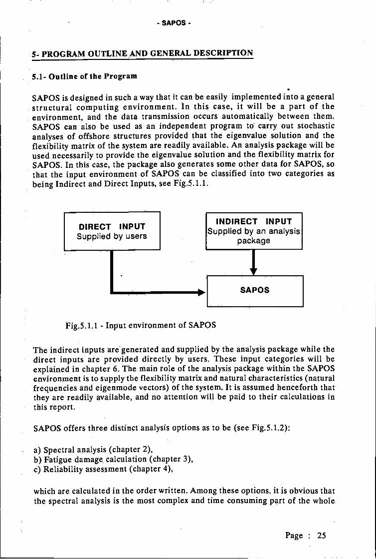
SAPOS is designed in such a way that it can be easily implemented into a generalstructural computing environment. In this case, it will be a part of theenvironment, and the data transmission occurs automatically between them.SAPOS can alsO be used as an independent program W carry out stochasticanalyses of offshore structures provided that the eigenvalue solution and theflexibility matrix of the system are readily available. An analysis package will beused necessarily to provide the eigenvalue solution and the flexibility matrix forSAPOS. In this case, the package also generates some other data for' SAPOS, sothat the input environment of 'SAPOS can be classified into two categories asbeing Indirect and Direct Inputs, see Fig.5.1.1.
DIRECT INPUTSupplied by users
i
Fig.5.11 - Input environment of SAPOS
The indirect inputs are generated and supplied by the analysis package while thedirect inputs are provided directly by users. These input categories will beexplained in chapter 6 The main role of the analysis package within the SAPOSenvironment is to supply the flexibility matrix and natural characteristics (naturalfrequencies and eigenmode vectors) of the system. It is assumed henceforth thatthey are readily available, and no attention will be paid to their calculations inthis report.
SAPOS offers three distinct analysis options as to be (see Fig.5.1.2):
Spectral analysis (chapter 2),Fatigue damage, calculation (chapter 3),Reliability assessment (chapter 4),
Which are calculated in the order written. Among these options, it is obvious thatthe spectral analysis is the most complex and time consuming part of the whole
Page : 25
INDIRECT INPUTSupplied by an analysis
package
SAPOS
- SAPOS -.
program. A special algorithm is .thérefore developed and used. in SAPOS tooptimize the calculation of the spectral analysis which is outlined mainly in thefollowing paragraphs.
SPECTRAL ANALYSIS
FATIGUE DAMAGE CALCULATION
RELIABILITY CALCULATION
Fig.5.1.2 - Analysis options of SAPOS in the calculation order.
The essence of this algorithm is suchthat the stress transfer function is calculateddirectly from transfer functions of member wave fórces without calculating thedisplacements. The flow diagram of the calculation procedure is shown inFig.5.1.3 where the eigenvalue solution is assumed to be available using ananalysis package.
As it might be realized from Fig.5.1.3, the algorithm is based on calculatingcontributions of all loaded members. The contribution of a member is merelycalculated as a vector product of transfer functions of member-wave-forces andsome total response terms (dynamic and quasi-static) that explained in chapter 2.The final stress transfer function is then obtained by superimposing thecontribution of the fixed-end member-forces, see Eq.(2.4.4), to the cumulativecontributions of members. This is formulated by Eq.(2.4.5).
The quasi-static part of the response is calculated from the syste.m flexibilitymatrix according to Eq.(.2.4.7a). This part of the response is frequencyindependent. Therefore, it is calculated once, and used whenever needed. In thecase of the reliability calculation, the quasi-static response containsuncertainties regarding only the stiffness matrix. This property is considered inthe numerical evaluation of the partial derivatives of the limit state function g(),see chapter 4, to make a shortcut in the. overall computation.
The dynamic part of the response is calculated according to Eq.(2.4.8). Unlikethe quasi-static part, it is frequency dependent and requires the eigenvaluesolution. The flow diagram of the calculation is shown in Fig.5.1.4.
As written in Eq.(2.4.8), and also illustrated in Fig.5.1.4, the dynamic part of theresponse is calculated by superimposing modal contributions. A modalcontribution is obtained from a triple combination of the member eigenmode
Page : 26

,vector, a modal stress and the modified modal transfer function given byEq (2 2 2) When the reliability analysis is carried out, the dynamic response isstated in the uncertainty space that concerns only the stiffness, mass and dampingmatrices This fact is also accounted in the numerical calculation of the partialderivatives of the g(.) function.
I-
I
CONTRIBUTION TOSTRESS
TRANSFERFUNCTION
ISTRESS TRANSFER
FUNCTION
MODAL TRANSFERFUNCTION
- SAPOS -
EIG EN VALU E
SOLUTION
4
Fig.5.L3 - Flow diagram for the calcûlation of a stress transfer function.
y
MODALSTRESS
4
MODALCONTRIBUTION
IDYNAMIC
CONTRIBUTION
TRANS FERFUNCTION OF
MEMBER WAVEFORCE
CONTRIBUTION OFFIXED-END MEMBER
FORCES
IMEMBER
EIGENMÖDE
Fig.5. 1.4- Flow diagram for the càlculation of the dynamic part of the response.
Page : 27
fDYNAMIC
CONTRIBUTIONSTATIC
CONTRIBUTIONG)
EG)E-c
'1SUPERPOSITION
a)-co

As the response components are concerned, it is worth noting in this context thatthé total response term (quasi-staticand dynamic), see Eq.(2.4.6), is independentof wave loadings This leads to a shortcut in the computation time when a multi-directional wave climate is taken intO account in the analysis since the totalresponse term remains unchanged by the variation of the wave direction. This isespecially remarkable in the reliability analysis.
Having calculated the stress transfer function, s outlined above, the spectrumand spectral moments of the stress process, the fatigue damage and the reliabilitycalculations are carried out consequently. The flow diagram Of the calculations isshown in Fig.51.5.
STRESS TRANSFERFUNCTION
RELIABILITYCALCULATION
NO
- SAPOS-
STRESS SPECTRUM I SPECtRUM
STRESS SPECTRALMOMENtS
FATIGUE DAMAGE
YES
RELIABILITY INDEX fi
YES
NO
SEA
Fig.5.1.5 - Flow diagram for the fatigue damage and the reliability calculations.
For a given sea spectrum, either P.M. or JONSWAP, the stress spectrum iscalculated using Eq (2 5 2) The stress spectral moments are calculated from thefrequency intégration given by Eq.(2.5.1). Then, the calculation of thecumulative fatigue damage is carried out following the procedure explained in
Page : 28
SAPOS -
chapter 3. If, however, the relIability analysis is concerned , it is carried out usingthe procedure explained in section 4 2 In this case, the calculation is repeateduntil a required convergence is obtained..
5.2- General Description
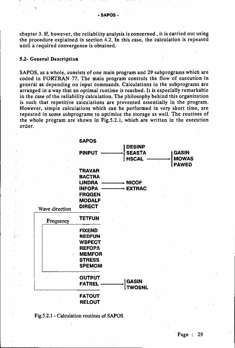
SAPOS, as a whole, consists of one main program and 29 subprograms which arecoded in FORTRAN 77 The main program controls the flow of execution ingeneral as depending on input commands. Calculations in the subprograms arearranged in a way that an optimal runtime is reached It is especially remarkablein the case of the reliability calculation. The philosophy behind this organizationis such that repetiti.ve calculations are prevented essentially in the program.However, simple calculations which. can be performed in very Short time, arerepeated in some subprograms to optimize the storage as well The routines ofthe whole program are shown in Fig 5 2 1, which are written in the executionorder.
Fig.5.2. i - Câlculation routines of SAPOS
Page : 29
SAPOSDESINP
PINPUT SEASTA GASINHSCAL MOWAS
PAWEDTRAVARBACTRALÍNDRA NICOF.
INFOPA 'EXTRAC- -
FROGENMODALF
Wave direction DIRECT
Frequency TETFUN
FIXENDREDFUNWSPECTREFOPAMEMFORSTRESSSPEMÖM
OUTPUTFATREL GASIN
TWOSNL
FATOUTRELOUT

In the program, some simplifications (some precalculated values) are also madeusing SI-UNITS (METER for length, SECOND for time, kg for mass) so that thisunit system must be maintained throughout an analysis option.
Since calculations. in the whole program are .arranged in an optimal way, it is verydifficult to explain specific tasks of the program routines. Nevertheless, theirprinciple duties are shortly described below to give a general idea.
SAPOSPINPUT
DESINP
SEASTAHSCAL
GASINMO WAS
PAWED
MODALF:
DIRECT
TETFUN
- SAPOS -
Main program.Reads input commands and data. Calculates member diameters frommember properties and member direction cosines.It is activated only in the case of the reliability analysis to readinformation about design variables.Reads data of the sea spectrum and the sea state.It is activated only when using a continuous long-term distributionof the sea state. It evaluates H, and also T in the case of a jointdistribution, at integration points in the long-term.Contains abscissa and weight factors of Gauss integrations.Calculates moments of conditional and marginal distributions of I-Isand T from a provided scatter diagram. They are used to find outcontinuous distribution functions for these measures.It is used to calculate the parameters of the Weibull distributiongiven that the mean, variance and the third central moment areknown.It is activated only in the casé of the reliability analysis. Itcalculates independent pairs of the correlated random variables.It is also activated only in the case of the reliability analysis. Itcalculates equivalent normal distributions of non-normal variables,and evàluates original (correlated) variables at the increments of thecorresponding basic variables.Calculates linearized wave force constants of loaded members.Contains coefficients of a special numerical integration process tocalculate variance of the water velocity in the wave direction.Calculates coordinate transformation-matrices of stress members. Italso calculates partly the static part of the response.Extracts coefficient matrices, [A], of member displacements fromthe flexibility matrix, see Eq.(2.4.7b)Generates frequency integration points to be dependent on naturalfrequencies. Here, an automatic generation is applied, whichproduces minimal frequency points resulting in accurateintegrations.Calculates member modal forces (member internal forces undereigenmode configurations), modal transfer functions, and, theproducts of these two items.It is activated oniy in the case of multi-directional sea states. Itcalculates abscissas and weight factors of the numerical integrationin the wave direction.Evaluates wave direction-functions of linearized drag forces of
Page : 30
TRAVAR
BACTRA:
LINDRANICOF
INFOPA
EXTRAC
FRQGEN:
- SAPOS -
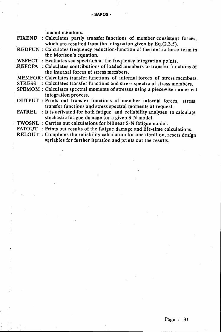
loaded members.FIXEND Calculates partly transfer functions òf member consistent forces,
which are resulted from the integration given by Eq.(2.3.5).REDFUN: Calculates frequency reduction-function f the inertia force-term in
the Morison's equation.WSPECT Evaluates sea spectrum at the freqûency integration points..REFOPA Calculates contributions of loaded members to transfer functions Of
the internal forces of stress members.MEMFOR: Calculates transfer functions of internal forces of stress membersSTRESS Calculates transfer functions and stress spectra of stress members.SPEMOM: Calculates spectral moments of stresses using a piecewise numerical
integration process.OUTPUT: Prints out transfer functions of member internal forces, stress
transfer functions and stress spectral moments at request.FATREL It is activated fOr both fatigue and reliability analyses to calculate
stochastic fatigue damage for a given S-N model.TWO SNL Carries out calculations for bilinear SN fatigue model.FATOUT Prints out results of the fatigue damage and life-time calculationsRELOUT: Completes the reliability calculation for one iteration, resets design
variables for further iteration and prints out the results.
Page : 31
- SAPOS -
6- PROGRAM. INPUTS
As mentioned in the previous chapter, SAPOS is used in co-operation with ananalysis package which provides mainly eigenvalue solution and the systemflexibility matrix. Although it may improve the runtime efficiency,implementation of SAPOS into an analysis package is not essentially needed. Inthis case, SAPOS receives some commands and data from a file which will beproduced by the package used. This kind of input to SAPOS is named here asIndirect Inputs, because they are generated by another program. However, someextra inputs, which are needed for the stochastic analysis, must also be supplieddirectly by users. Such inputs are named here as Direct Inputs. Inputs to theanalysis package are not considered in this manual since they may vary frompackage to package. Here, attention will be paid only to the inputs of SAPOS.Although not necessary, it may be recommended that the same data file is usedfor both the indirect and direct inputs. In this case, the former precedes thelatter, because the program requires the indirect inputs first, then the directinputs. These input items are explained in this chapter in detail.
6.1- Indirect Inputs
As noted above, the indirect inputs are defined to be those generated by ananalysis package. These are not only the results of the eigenvalue solution andthe system flexibility matrix but also some other data concerning submergedmembers and joints, as well as generalized masses. These data and relatedinformation will be written to a data file by the package used. Forms of the dataand information will be explained below in this section in detail. However, it isworth noting in this context that the package to be used must be adapted to meetrequirements of these inputs. In the following, instructions (commands) andforms of data are presented, where the uppercase characters need .to be specifiedwhile the rest with lowercase characters are optional. It is also important that allcommands must be specified starting from first columns of relevant records. Textwritten in brackets, if stated, can also be used as an alternative commandstatement. Data inputs are specified succeeding the command specification.Unless it is stated otherwise, the order of input items (command +. data) can bechanged if re4uired. First characters in all data records must be kept empty(blank). This is especially needed to identify data and command records.Following each input item examples are presented to demonstrate how the inputsare specified.
6.1.1- INCidences of submerged membersmijkwhere,m : an integer denoting a submerged member,i : an integer denoting the number of member ends (i = 2),j : an integer 'denoting the joint number of the first end of the member m,
Page : 32

- SAPOS -
k: an integer denoting the joint number of the second end of themember m.
This command is used to input submerged members. One data record isused for orte member. Data will be repeated for all submergéd members.The format specification is : FORMAT(415).
Example:
INCIDENCES OF SUBMERGED MEMBERS / ELEMENTS
and So on
6.1.2- BOOkkeeping degrees of freedOm of submerged jointsm3 ml m2
where,ml: an integer denoting a joint number,
an integer denoting a local degree of freedom at the joint ml (it isa number between 1 and 6),an integer denoting the global degree of freedom corresponding tom2.
This command is used to keep track of local and global degrees offreedom of submerged joints It provides the list of connections betweenlocal and global degrees of freedom of joints as demonstrated by thefollowing example which corresponds to Fig.6.l.2. Data will be repeatedfor all lOcal degrees of freedom of all submerged joints. The formatspecification is : FORMAT(3I5).
Example:
BOOKKEEPING DEG. OF FREE. OF SUBMERGED JOINTS
Page : 33
72182292310
2
11 2 .5
U 2 613 3 1
14 3 215 3 316 3 417 3 518 3 6
9210910 2 11 1011 2 12 11

-. SAPOS -
6.1.3- COOrdinates olsubmerged jointsn x y z
where,n an integer denoting a joint in water,x : X coordinate of the joint n,y : Y coordinate of the joint n,z : Z coordinate of the joint n, measured from the still water level, and
assumed () in upward direct jon.
This command is used to input global coordinates of submerged joints.Here, X, y and z are floating point constants. One record is used for onejoint Data will be repeated for all submerged Joints The format isFORMAT(15,3F13.3).
Page 34
Local degrees of freedomat a joint
Fig.6.1.2- Demonstration of bookkeeping degrees of freedom of submergedjoints.
m3 ml rn2
7 2 I8 2 29 2 310 2 411 2 512 2 613 3 1
14 3 215 3 316 3 417 3 5.
18 3 6

Example:
COORDINATES OF SUBMERGED JOINTS
and so on
6.1.4- DiSplacements (EIGENMode vectors) of submerged jointsmi ux uy uzj rx ry rz
where,m: an integer denoting an eigenmode,j : an integer denoting a joint in water,ux, uy, uz : floating point constants denoting components of normalized
translational eigenvector in the global X, Y and Z directionsat the jo!ntj,
rx, ry, rz : floating point constants denoting components of normalizedrotational eigenvector in the global X, Y and Z directions atthe joint j,
This command must succeed the command, COORDINATES OFSUBMERGED JOINTS presented in 6.1.3. It is used to input eigenmodevectors of submerged joints, which must be normalized to i. before theyare specified. At a joint, first the translational and then the rotationaleigenmode vectors have tobe specified in two subsequent data records.This process of one eigenmode specification will be repeated until thedata of all submerged joints are input. The same process, as a whole, willalso be repeated until all eigenmode vectors are input in th.e increasingorder. The data are Specified in the free format, but must be floatingpoint. It is important, however, that eigenmode vectors need to bespecified with sufficiently significant digits to obtain accurate modalstresses.
Example:
EIGENMODE VECTORS OF SUBMERGED JOINTS1
- SAPOS -
Page : 35
16 1.852 -1.070 -9.10617 -1.852 -1.070 -9.10618 0.000 2.139 -9.10619 5.373 -3.102 -16.14620 5.373 -3.102 -16.146
9 0.1806886E + 00 0.1029443E +00 -0.8314867E-069 -0.1487340E-01 0.2610410E-01 -0i160778E-0110 0.1272312E +00 0.7246580E-01 -0.8448677E-0610 -0.1277629E-01 0.2242371E-01 -0.1096719E-01
6.1.5 MODal (GENeralized) massesn g
where,n an integer denoting an eigenmode,g a floating point constant denoting the generalized (modal) mass for
the eigenmode n.
This command is used to input generalized masses of the structure. Onerecord is used for one eigenmode Data will be repeated until alleigenmodes, which are taken into accöunt, are specified. The formatspecification is : FORMAT(I5,E15.8).
Example
GENERALIZED MASSESI 0.24017E±062 0.29896E ±06
and so on
6.1.6- NATural frequencies (EIGENVa1ues)n w
where,n : an integer denoting an eigenmode,w :a floating point constant denOting the natural frequency of the mode
n in (rad/sec).
This command is used t input natural frequencies of the structure. Onerecord is defined for one eigenmode. Data will be repeated until allmodes are specified The format specification is FORMAT(15,E15 8)
Example:
NATURAL FREQUENCIES1 3.228632 3.26338andsoon
Page 36
- SAPOS -
2
and so on
9 -0.1179547E±QQ 0.2Ú69789E+00 -0.5567765E-039 -0 2995057E-01 -0 1706761E-01 -0 1379644E-0410 -0.8300674E-01 0.1456519E +00 -0.5443799E-0310 -0 2572156E-01 -0 1465780E-01 -0 1292325E-04
- SAPOS -
6.1.7- PROperties of submerged membersma xy z t
where,m: an integer denoting a submerged member,a : cross-sectional area of the member m,x : Ix, torsional constant Of the member cross-section (polar inertia
moment for circular cross-section),y ly, flexural inertia moment of the member cross- section about the
local Y axis,z : Iz, flexural inertia moment of the member cross section about the
local Z axis,t : average thickness of marine growths on the member in as shown in
fig.6.1.7.
PROPERTIES OF SUBMERGED MEMBERS9 O.2100E+O0 02321E+0O 0.1160E+00
lo 0.2100E+00 0.2321E+00 0.1160E+0011 0.2529E +00 0.2756E +00 0.1378E + 0012 0.2529E +00 0.2756E +00 0.1378E +0013 O.1683E+OO 0A871E+O0 0.9353E-014 0.1683E + 00 0.187 lE + 00 0.9353E-01
and so on
(thickness of marine growth)
Fig.6.1.7 - A tubular member cross-section and the average thickness ofmarine growths
This command is used to input seçtional properties of, submergedmembers, as well as average thicknesses of marine growths on membersÏn the general form written above, a, x, y, z and t aré floating pointconstants. This command and corresponding data are produced by ananalysis package, except thicknesses of the marine growths which mustbe later externally added on the data records. One record is used for onemember so that the number of data records are equal to the number ofsubmerged members. The format specification is : FORMAT(15,5E12.4).
Example:
Page 37
0.1160E + 00 0.200.1160E +00 0.200.1378E + 00 0.200.1378E + OÙ 0.200.9353E-01 0.200.9353E-0 i 0.20
i23456789.
- SAPOS -
X
symmetric
xxxxxX X X. X
X x. x xxx xxx xx x x x x x,x xx X X .X X
x x X X X X Xxxx xxx xx x x x X xX * xx xxx
X
.1.8- FLExibility matrix (stored columnwise from diagonal terms)size of flexibility matrix: ncolumn ml rn2list
where,n : an integer denoting total number of columns, or rows, of the
flexibility matrix,ml an integer referring to a column number of the flexibility matrix,m2 : an integer denoting the band-width (number of data to be read) of
the column ml, see also Fig.6.l.8 below,list : a list of data of the flexibility matrix in column ml, which are equal
to m2.
ml --. 1 2 3 4 5.6 7 8 9 n
m2 8696.. .23. 1
Fig.6.L8 -, Flexibility matrix and definition of input parameters, n, mland m2.
This command is used to input system flexibility matrix (inverse of thestiffness matrix). Succeeding the command- record, Size of the flexibilitymatrix is specified in a separate record. The text i.n this record is optional.If stated, it must precede the size, n, of the matrix. At least one blankcharacter (a space) is required between the text and n. Each column ofthe matrix and the number of contained data must be specified in a recordbefore the data are input. The format of this specification isFORMAT(A6,215). Then, the flexibility matrix is written columnWisestarting from diagonal terms in the free format specification.
Page : 38

- SAPOS -
Example:
FLEXIBILITY MATRIX (STORED COL. FROM DIA. TERMS)SIZE OF FLEXIBILITY MATRIX 174COLUMN 1 174
O 471362E-06 -0 129732E-07 O 203557E-07 O 163327E-110.203543E-07 0.130085E-07 .393349E-06 -0.909128E-07
COLUMN 170 50.554654E-07 -0.127545E-10 0.286413E-13 0.165365E-130.141438E-09
COLUMN 171 40.73333E-O6 0.9203 18E-14 0.250183E-14 959420E-17
COLUMN 172 30.735281E-08 -0.649583E-08 -0.235719E-12
COLUMN 173 2O 148532E-07 -0 136096E-12
COLUMN 174 1
0.378814E-08
Page : 39
6.2- Direct Inputs
In addition to the inputs presented above there are also some extra inputs neededfor a stochastic analysis option to be carried out by SAPOS. These inputs aresupplied directly by users. Therefore, they are called in this report as DirectInputs. Aithough not necessary, it is recommended that the Same data file is usedfor both the indirect and the direct input categories. Since the indirect inputs aregenerated. by computers they precede the direct inputs. Before the input itemsare presented, the following conventions which are used in general are made
The uppercase characters written in command records must be specifiedwhile the lowercase characters are optional.Alternative statements of commands are written in brackets, if. they exist.Commands can be written anywhere in records and, if required, their ordercan be interchanged unless it is noted otherwise.Texts and data, or multiple data, in a record must be separated from eachother by at least one blank character.
Demonstrations of these inputs are presented after each item is explained.
6.2.1- DAMping ratioslist
This command is used to input critical damping ratios. Since dampingratios are required only in the response analysis, they are specified in thiscategory of the inpi.its. The list contains a list of data for the criticaldamping ratios written in the free format specification. The number öfdata are equal to the number of eigenmodes considered.
Example:
DAMPING RATIOS0.01 0.01 0.01
SAPOS -
6.2.2- MATerial constantsEG
This command is used to input the elasticity modulus (E) and the Youngmodulus (G) of the structural material. It is assumed that the samematerial is used for the whole structure since the foundation isrepresented by massless springs. E and G are specified in free format.
Example:
MATERIAL CONSTANTS21.OE+10 8.1E+10
Page 40
6.2.3- LOAding propertiesrw cm cd
where,s
rw : density of water5cm : inertia force coefficient of the Morison's equation,cd : drag force coefficient of the Mörison's equation.
This command is used to input water density and wave forcé coefficients,cm and Cd, in the free format specification. If this command is notspecified, rw = 1024 kg/rn3, cm = 2.0 and cd 1.3 will be used bydefault.
Example:
LOADING PROPERTIES1024.0 1.8 0.9
- SAPOS -
[UNI-6.2.4- WAVe properties
[[MULti-][nm ni ndl
directional sea
where,nm : number of main wave directions,ni : number of individual wave directions,nd : degree of the spreading function.
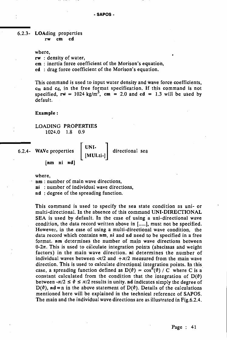
This command is used to specify the sea state condition as uni- ormulti-directional. In the absence of this command UNI-DIRECTIONALSEA is used by default. n the case of using a uni-directional wavecondition, the data récord written abOve in [ ], must not be specified.However, in the case of using a multi-directional wave condition, thedata record which contains nm, ni and nd need to be specified in a freeformat. nm determines the number of main wave directions between0-2r. This is used to cálculate integration points (abscissas and weightfactors) in the main wave direction. ni determines the number ofindividual waves between -r/2 and ±r/2 measured from the main wavedirection This is used to calculate directional integration points In thiscase, a spreading function defined as D(i) = cos() / C where C is aconstant calculated from the condition that the integration of D(t)between -r/2 'r/2 results in unity. nd indicates simply the degrec ofD(i), ndn in the above statement of D(i). Details of the calculationsmentioned here will be explained in the technical reference of SAPOS.The main and the individual wave directions are as illustrated in Fig.6.2.4.
Page : 41
Fig.6.2.4 - Main and individual wave directions
The directional integration with respect to individual waVes is carried outonly if both values of ni and nd are set to be greater than 1. OtherWise, nospreading function is taken into account In this case, only one individualwave condition is considered, which coincide with the main wave Asbeing independent of individual waves, a number of main waves can bespecified if required This command can be used in different ways asdemonstrated below.
Examples:
WAVE PROPERTIES, UNI-DIRECTIONAL
WAVE PROPERTIESUNI-DIRECTIONAL
UNI-DIRECTIONAL SEA.
WAVE PROPERTIES, MULTI-DIRECTIONAL142WAVE PROPERTIESMULTI-DIRECTIONAL210
6 MULTI-DIRECTIONAL SEA461
Page 42
£
- SAPOS -
An individual wave direction
Main wave direction

6.2.5- MAIn wave direction: to
This command is used to specify the direction angle of the main wave.The direction angle of the main wave is measured from the global X axis,see Fig.6.24. Here, to is a floating point constant denoting the value ofthe directión. angle in degrees. It must be specified as the last item in therecord. In the absence of this command to = 0.0 is used by default. In thecase of using multi- directional main waves, this command determines aninitial direction from which the integration domain is defined to be 0-2r.Since the integration domain is a complete cyde, such a directional shiftdoes not affect the results.
Example:
MAIN WAVE DIRECTION TO = 45.0
6.2.6- GAUss points for frequency integration: np
This command is used to specify the number of Gauss points for thenumerical integration in the frequency domain. The frequency domainintegration is carried out to calculate stress spectral moments given byEq.(2.5!1). np is an integer constant denoting the number of Gauss points.It must be defined between 3 np 7. It can be specified anywhere onthe record provided that it begins with the first numçrical character. Ifthis command is not present, it is assumed by default that np =3.
Example:
GAUSS POINTS FOR FREQUENCY INTEGRATION, N = 4
- SAPOS -
This command is used generally to specify the type of the analysis, whichis either spectral, fatigue or reliability, and the type of response which iseither static, dynamic or static + dynamic. Here, STA means only the staticcontribution and DYN means only the dynamic contribution. If both STAand DYN (STA + DYN) are specified, the complete response behaviour istaken into account. The following fOrm of the command can also beaccepted in two or more records instead of one.
SPEctral
FATigue analysis, - - on the first record,RELiability
Page : 43
[SPEctral ] STAtic
6.2.7- FATigue analysis DYNamic contributionRELiabilityJ STAtic + DYNamic
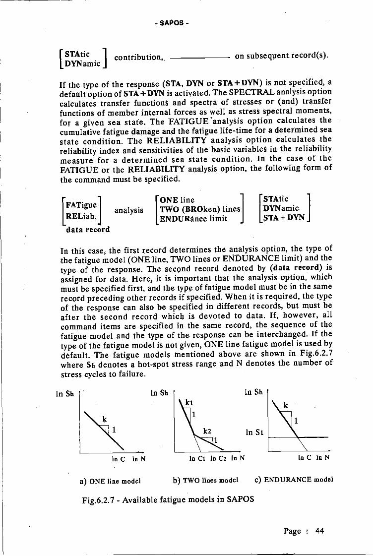
in Sh
I STAtic I contribution, on subsequent record(s).
If the type of the response (STA, DYN or STA +DYN) is not specified, adefault option óf STA + DYN is activated. The SPECTRAL analysis optioncalculates transfer functions and spectra of stresses or (and) transferfunctions of member internal forces as well as stress spectral moments.,for a given sea state. The FATIGUE analysis option calculates thecumulative fatigue damage and the fatigue life-time for a determined seastate condition. The RELIABILITY analysis option calculates thereliability index and Sensitivities of the basic variables in the reliabilitymeasure for a determined sea state condition. In the case of theFATIGUE or the RELIABILITY analysis option, the following form ofthe command must be specified.
DYNamic
In this case, the first record determines the analysis option, the type ofthe fatigue model (ONE line, TWO lines or ENDURANCE limit) and thetype of the response. The second record denoted by (data record) isassigned for data. Here, it is important that the analysis option, whichmust be specified first, and the type of fatigue model must be in the samerecord preceding other records if specified. When it is required, the typeof the response can also be specified in different records, but must beafter the second record which is devoted to data. If, however, allcommand items are specified in the same record, the sequence of thefatigue model and the type of the response can be interchanged. If thetype of the fatigue model is not given, ONE line fatigue model is used bydefault. The fatigue models mentioned above are shown in Fig,6.2.7where Sb denotes a hot-spot stress range and N denotes the number ofstress cycles to failure.
- SAPOS -
In Sb
FATigue[RELiab.
analysisONE lineTWO (BROken) linesENDURance limit
STAticDYNamic.STA+DYN
data record
in C in N In Ci in C2 in N in C in N
a) ONE une modei b) TWO lines modei c) ENDURANCE model
Fig.6.2.1 - Available fatigue models in SAPOS
Page 44
- SAPOS -
The (data record) contains some floating point constants depending onthe type of the fatigue model used. These constants, which are in the freeformat specification,, are presented below for each type.
ONE line fatigue model:inC k b d
TWO lines fatigue model:mCi ki inC2 k2, b
) Fatigue model with ENDURANCE limit:inC k Si b d
where the notations are shown in Fig.6.2.7, except b and d. Hère, bdenotes the mean valué of the basic variable, X14, of the damagecorrection factor given by Eq.(4.1.3.2). This mean value is a function ofthe slope (k) of the S-N line used. For k=3.80, a value of b= 0.15 isobtained. For further information, users should cOnsult Ref.[8]. For anarrow-band process, b = 0.0 will be used, in which case the associateddesign variable is considered to be deterministic. The constant, d, inabove lists denotes the mean value of the reference damage, Df, seesection 4.1.3, which shows considerable variations in practice. When the.cumùlative damage reaches this value, it is said that failure occurs. Forpractical purposes, d= 1.0 is commonly used.
Examples:
1- FATIGUE ANALYSIS, ONE S-N LINE96.05 4.0 0.17 1.0STATIC CONTRIBUTION
FATIGUE ANALYSIS, STATIC CONTRIBUTION96.05 4.0 0.17 1.0
ELIABILITY ANALYSIS, TWO S-N LINES8587 3.8 96.05 4.6 0.0 1.0STATIC CONTRIBUTIONDYNAMIC CONTRIBUTION
RELIAB. ANAL., BROKEN S-N LINE, STA. AND DYN. CONT.85.87 3.8 96.05 4.6 0.0 1.0
Hére, the examples 1 and 2, and 3 and 4 are equivalent. As explainedabove some other combinations of the commands can be made.
Page 45

FORCEs6.2.8- LIST STRESses
SPECTra! moments
- SAPOS -.
for the sea state h (and t)
Where, h and t are floating point constants denoting respectively values ofthe significant wave height and, if applicable, the mean zero crossingperiod of waves in the sea state.
This command is used to activate user controlled output options iñaddition to standard oútputs which will be explained later. The command,FORCES, is used to prInt out complex transfer functions of memberinternal forces. The command, STRESSES, is used to print out modulusof transfer functions and (or) spectral values of hot-spot stresses at .givenlocations while the command, SPECTRAL MOMENTS, is used for theoutput of the stress spectral moments for all sea states involved. Thecommand,, STRESSES, can be used with two options as specified by,
I TRANsfer functions iLIST STRESses
L SPECtral values j for the sea state h (and t)
The command, TRANsfer functions, is used to print out the transferfunctions while the command, SPECtral values, is used for the output ofthe spectra of. stresses. A combination of these two commands is alsopossible. In this case, the transfer functions and the spectral values ofstresses are both printed out. If one of these options is not specified,, it isassumed by defäult that SPECtral values is activated.
The first encountered numerical value in the record is assigned for thesignificant wave height, Hs, and the second one is used for the meanperiod of Waves, T, when a two parameters sea state (sea state with ascatter diagram) is applied. If, however, h (and t) is (are) not specifiedthe values of H=2.O m. and T=5.O sec. are used by default. It isimportant that, in the case of multiple LIST command, the last specifiedh and 't values overwrite préviously defined values. This will be clarifiedby the examples below. In the absence of this command some standardoutputs will be printed out, see chapter 7. When only the spectral analysisis carried out and this command is not provided, then LIST STRESSSPECTRAL VALUES and LIST SPECTRAL MOMENTS will beactivated by default. See section 1.2 for further information aboutoutputs.
Page 46
6.2.9-
Examples:
LIST FORCESLIST STRESSESLIST SPECTRAL MOMENTS
In this example, transfer functions of forces and stresses are printed oUtfor H 2m. and T = 5sec.
LIST FORCES FOR HS 4.0 TZ 8.0LIST STRESSES FOR HS 3.0 TZ 90LIST SPECTRAL MOMENTS
In this example, forces and stresses are printed out for H =3.0 m. and9.0 sec; irrespective of what specified in the first record.
LIST FORCESLIST SPECTRAL MOMENTS 1.50 4.20LIST STRESSES
In this example, forces and stresses are printed out for H = 1.50 rn .andT = 4.20 sec., although they are defined in the command of SPECTRALMOMENTS Spectral moments are printed out in any case for all H andTz values;
- SAPOS -
SEA properties
[y a Ob]{a,7 nh}Info. Ree.list
[P.M.[JONswa
spectrum, SCAtter (DIAgram)
where, y, 0a and Cb are floating point constants denoting parameters ofthe JONSWAP sea spectrum, see Eq.(4.1.2.7). These parameters arespecified in free format, when the JONSWAP spectrum is used If it is so,they must be specified in the secönd record. [...] denotes a record thatused in the case of the JONSWAP spectrum. {...} denotes also anòtherrecOrd that used only if one parameter sea spectrum is applied.Otherwise, it is omitted Herein, a is a floating point constant whichdenotes the shape parameter of the spectrum used, see Eqs.(4;1.2;4) and(4.1.2.7), nh is an integer constant which denotes the number of Hvalues. Both a,7 and nh are specified in free format. he last two items,Info.Rec. and list, must be specified in any case. Info.Rec. is aninformation record and list is a data record which will be explained later.
Page : 47
- SAPOS -
This command is used to specify a random sea condition, where P.M.denotes the Pierson-Moskowitz sea spectrum. It must. be specified afterthe specification of the analysis type, seê item 6.2.7. As it is seen, twospectral forms of the random sea are implemented with, or without, usinga scatter diagram identified by either SCA or DIA. If one of theseidentifiers of a scatter diagram is not included in the command, oneparameter sea spectrum is assumed by default. If the type of the seaspectrUm is not-specified, the P.M. sea spectrum is used by default as well.In the case of using a JONSWAP sea spectrum, the second recordindicated by [....] is assigned for some data of this spectrUm. In the case ofusing a one parameter sea spectrUm the third record indicated by {....}must alsó be specified, The records Info.Rec. and list are explainedseparately in two cases of using either one parameter or two parameterssea spectrum.
a- Using one parameter sea spectrum:
1- If Info.Rec. contains either WEIBu11 or LOGNormal, a continuousprobability density function (Weibull or Lognormal type) is used forthe marginal distribution Of Hs in the 1ngterm. In this case, aGaussian type integration is applied to calculate Eq.(3.4) in the long-term. The number of integration points are determined by nh writtenabove in {....}. The last item, list, contains the following data in a freeformat specification.
A B C for WEIBULL distribution,au C for LOGNORMAL distribution,
where, A, B, C, s and a are all floating point constants denoting theparameters of the corresponding distribution types, which are shownbelow in the functions.
C hA hACWeibull distribution: fHs(h) =j- ( ) exp(- ( ) )
i i lnh-p2Lognormal distrib. : fHs(h) - 2.ir a h
exp a ))
2 If InfO.Rec. does not contain either WElBull or LOGNormal, aWeibull type probability density function is used by default fOr themarginal distribution of iIs in the long- term.. In this case, discretevalues of Hs are used to calculate Eq.(3.4) applying a trapezoidal rule
Page : 48
SAPOS -
for the numerical integration. The list contains the following data infree format specifications.
A B Chi h2 h3 hn
where A, B, and C are floating pOint constants denoting the parametersof the Weibull distribution, which must be specified in the first recordof the list, hi, h2....., hn are also floating point constants denotingvalues of H specified in subsequent records of the list. More that onerecords for H values can be used, and a number of data on one recordcan be arbitrary, but must be between columns 1-80. The total numberof H values must be equal to nh defined above in {...}.
b- Using two parameters sea spectrum:
In this case, SCATTER DIAGRAM must be specified and the recordindicated by {....} must be dropped. If, Info.Rec. contains the followingcommands,
WEIBu11 iI and
I WEIBu11 iTZ [LoGNormalj distributionsHS LOGNOrmalJ
a continuous probability density function is used for the joint distributionof H and T in the long-term. In this case, a Gaussian type numericalintegration is applied to evaluate Eq.(3.4). The density function of thejoint distribution is calculated from,
fHs,Tz(h,t) = fTz(ttHs) fHs(h)
where fTz(t/Hs) is the conditional density function of T given that H isknown, and fHs(h) is the marginal density function of H. The types ofthese density functions are defined above after HS and TZ as being eitherWeibull or Lognormal. The parameters of the distribution functions Willbe calculated automatically from a provided scatter diagram in theprogram. The numbers of the numerical integration points in the H andT domains are respectively set equal to the numbers of H and T givenby the scatter diagram. The continuous formulation of the joint densityfunction is implemented only when the numbers of H and T are bothbetween 2 and 10. This restriction is made due to the fact that Gausspoints more than 10 are not implemented in the program. If the types ofH and T in the Info.Rec. are not completely specified, e.g. one of themis missing, then a discrete joint density function obtained from the scatterdiagram is applied. If it is required, the order of H and T may bechanged in the record. T and H5 values are first specified in the list.Then, numbers of occurrences of sea states (given H5 and T values) are
Page : 49
- SAPOS -
specified as integèr constants. All these data are given in free formatspecifications T and H are respectively input in the order of increasingvalues. The first recOrd in the list contains respectively the total numberof T as an integer and then its values as floating point constantsSimilarly, H is specified in the second record The third record and so onare devoted to data of the sea state occùrrences. These data aré input rowby row (sea state occurrences corresponding to T values for a given Hvalue) in the free format specification. This can be summarized as,
NT, (TZ(i), i 1 to NT) ... in first record of the list,NH, (HS(j), j = 1 to NH) in second record of the list,
(NOC(1,i), i i to NT) ... in súbsequent records...(NÖC(2,i), i = i to NT)
(NOC(NH,i), i =1 to NT)
where NT and NH denote respectively the numbers of Tz and H, TZ(.)and HS(.) arrays containing values of T and H, and NOC(.,.) is an arraywhich contains sea state occurrences, see also example 2 below.
Examples:
SEA STATE JONSWAP SPECTRUM3.3 0.07 0.090.0081 5WEIBULL DISTRIBUTION FOR HS0.60 1.67 1.20
SEA STATE P.M. SPECTRUM, SCATFER DIAGRAMHS AND TZ ARE DISCRETE8 3.50
5.30o04
39168643712
Page : 50
5.50 7.50 9.50 11.50 13.50 15.50 17.503.79 2.73 2.12 1.52 0.91 0.30
1 10 15 4 1 1 1
30 141 iiI 16 12 6 10104 225 89 22 12 6 ii337 358 96 34 17 9 16714 363 93 46 20 11 19982 272 8 51 23 13 17640 109 40 32 12 7 4
6.2.10- UNLoaded members numlist
where,num an integer denoting number of unloaded members,list : a list of integers containing unloaded members.
This command is used to specify unloaded members in water, which mayarise from the modelling of joint configurations in which some membersare. assumed to be unloaded. Although it is not necessary, this commandcan also be used fOr the members above water level. These members are,however, automatically implemented as unloaded members in theprogram. The first encountered numerical characters in the record areassigned for num. If num is not specified it is assumed by default that allsubmerged members are loaded, list contains unloaded members in thefree format specification. The number of data in the list must be equal tonu m.
Example:
UNLOADED MEMBERS 5
16 43 18 22 36
SAPOS -
6.2.11- STRess (FORce) locations nsmin j flSpa Sn sy sz
where nsm, m, j, nsp are integer constants defined as,nsm : number of stress members,m : a stress member,j : external joint number of the stress member m,nsp : number of stress points on the member cross- section,
and a, sn, sy, sz are floating point constants defined as,
direction angle of a stress point on the member cross-section,measured from local Y axis and defined in degrees, see Fig.6.2.11,
Sn : SCF of the normal force,sy : SCF of the bending moment (My) in local Y direction,sz : SCI? of the bending moment (Mz) in lOcal Z direction,
where SCF denotes stress concentration factor. For M and M, seeFig.6.2. 11.
This command is used to specify stress, or force, locations in the system..The first encountered numerical characters in the command record areassigned. for the number of stress, or force, members, nsm. If this is not
Page : 51
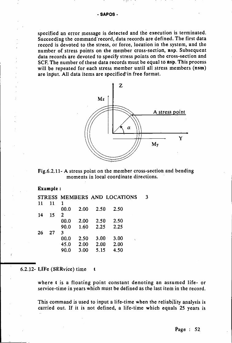
- SAPOS -
specified an error message is detected and the execution is terminatedSucceeding the command recórd, data records are defined. The first datarecord is devoted to the stress, or force, location in the system, and thenumber of stress points on the member cross-section, nsp. Subsequentdata records are devoted to specify stress points on the cross-section andSCF The number of these data records must be equal to nsp This processwill be repeated fOr each stress member until all stress members (nsrn)are input. All data items are speçifiedin free fOrmat.
6.2.12- LIFe (SERvice) time t
where t is a floating point constant denoting an assumed life- orservice-time in years which mUst be défined as the last item in the record.
This command is used to input a life-time when the reliability analysis iscarried out. If it is not defined, a life-time which equals 25 years is
Page 52
Fig.6.2. 11- A stress point on the member cross-section and bendingmoments in local coordinate directions.
Example :
STRESS MEMBERS AND LOCATIONS 311 11 1
00.0 2.00 2.50 2.5014 15 2
00.0 2.00 2.50 2.5090.0 1.60 2.25 2.25
26 27 300.0 2.50 3.00 3.0045.0 2.00 2.00 2MO90.0 3.00 5.15 4.50
- SAPOS -
assumed by default. In the case of the fatigue and spectral analyses, ifdefined, this command is ignored.
Example:
LIFE TIME 50.0
6.2.13- ITERation number of the reliability analysis, n
where n is an integer constant denoting the number of iterations of thereliability analysis, which must be defined as the last item in the record.
This command is used tó specify the number of reliability iterations, seesection 4.2. Thus, it is active only when the reliability analysis is carriedout. ¡fit is not specified 1 iteration (n 1) is performed by default. Thiscommand can be specified either within the command of DESIGNVARIABLES, see 6.2.14, or outside. If it is defined more than once, thelast one will be used as being active. In the fatigue and spectral analyses,if defined, this command will be ignored.
Example:
ITERATION NUMBER OF THE RELIABILITY ANALYSIS 3
6.2.14- DESign variables
This command is used to input coefficients of variations (u/u) anddistribution types of design variables. It is active only when the reliabilityanalysis is carried out. In the spectral and fatigue analysis, if defined, it isignored. This command will be terminated by a (I) as a first character inthe record. M mentioned above the command, ITERATION NUMBER,can also be defined under this command in the same way as presented.The input form of design variables is generally written as,
name y type
where,name : name of the uncertainty field,y : afloating point constant denoting coefficient of variation, u/4u,
of the design variable,type : distribution type of the design variable.
For each design variable the input will be repeated in the form givenabove. The name of the uncertainty field denotes a randóm field whereinuncertainties are represented by a design variable, e.g. the designvariable, Xk, represents uncertainties in the random field named asSTIFFNESS MATRIX, see section 4 11 A complete list of names of thedesign variables is presented below where the uppercase characters must
Page : 53

- SAPOS -
be specified while the lowercase characters are optional. The variablesenclosed by dots (....) are assumed to be correlated.
STIFfness matrix, correlated withMASS matrix
DAMPin g ratiosMARIne growth
ALFA (sea spectrum), correlated withGAMMa (sea spectrum)
INERtia forcesDRAG forcesSTREss concentration factor(FATIgue parameters),
correlatéd withKl
correlated withK2
DAMAge correcticn factor,REFErence damage,ENDUrancé lithit,,
this command is optional.
(see fig.6.2.7b)
(see fig6.2.7b)
see Eq.(4.1.3.2)see section 4.1.3see section 4.1.3
The above names with corresponding data and types can be specified inany Order. The distribution types must alsO be specified by alphabeticalcharacters. The following types, where the uppercase characters arecompulsory while the rest are optional, are implemented iii SAPOS.
De te rminis ticNormalLögnormalGamma
If a design variable is considered as deterministic, it must be declaredeither by D in type or y = O O in data If the type is not specified at all, itis assumed by default that the variable is also deterministic. As notedbefore, a deterministic design variable of the damage correction factor isimplemented, if its mean value is set to zero (narrow-band process).
For the correlated variables, correlation coefficients must be specified inthe form Written below as similar to above forms.
Page : 54
- SAPOS -
(CORRelation coefL), this command is optionalRO STiffness (MAss) matrix rsRO ALfa (GAmma) raRO LNC1 (Ki) rlRO LNC2 K2) r2
where rs, ra, rl and r2 are floating point constants which denotecorresponding correlation coefficients. This input is identified by RO,and then by one of the names of the correlated variables Alternativeidentifiers of names are written above in () Following the identifiers thecorrélation coefficients must be specified as being ast items in records.The correlated variables are assumed to be normally distributed, unlessone of them is declared as to be deterministic. In the analysis, onlyassociated design variables need to be specified as depending on thefatigue model and the sea spectrum used. However, if all variables arespecified, unnecessary variables will be ignored. For the necessary andunnecessary variables, see chapter 4.
Example:
DESIGN VARIABLESSTIFFNESS MATRIX 0.25 NMASS MATRIX 0.20 NDAMPING RATIOS 0.40 LMARINE GROWTHS 0.25 GALFA IN SEA SPECTRUM 0.15 NGAMMA IN JONS WAP SPEcTRUM 0.25 NINERTIA FORCES 0.20 LDRAG FORCES 0.20 GSTRESS CONT. FACTORS 0.45 DFATIGUE PARAMETERS optionalLNC1 0.024 NKl 0.026 NDAMAGE CORRECTION FACT 030 LREFERENCE DAMAGE 0.25 NCORRELATION COEFFICIENTS optionalRO STIFFNESS AND MASS 0.40RO ALFA AND GAMMA 0.94RO LNC1 AND Kl 0.97/ end of design-variables input.
Page : 55
SAPOS offers very friendly and self explained outputs which are very clear andconcise as printed out in tabulated forms. It is designed that the inputs are firstprinted out automatically to check the data, except the stiffness matrix since itrequires a large number of space. The outputs may be considered in twocategories as being Standard and user controlled. Standard outputs are defined asbeing those printed out automatically without user's intervention. Usercontrolled outputs are those printed out only when a LIST command, see 6.2.8 ofthe previous chapter, is specified.
7.1- Standard Outputs
The standard outputs are dependent on the analysis type in general, but incommon, some frequency blocks which are generated in the program for anefficient frequency integration are printed out first. Each frequency block istreated internally as an integration subregion where a Gaussian integrationprocedure is applied, see the input command 6.2.6. Then, the result of totalintegration, is obtained by superimposing individual integrations of thesubregions.
In the case of the spectral analysis, if a LIST command is not provided, spectralvalues and spectral moments of stresses will be printed out by default for aspecified sea state, and for each wave direction if applicable. Spectral values atstress locations on a cross-section of a given stress member will be tabulated foreach location against frequencies. This process is repeated for all stress membersand joints which are specified in the input.
In the case of the fatigue analysis, results of the damage calculation, for T i sec.,are listed for all stress locations and sea states. In the list are also presentedstress concentration factors, mean frequencies of zero-crossings and maxima ofstresses, and cumulative damages. This output list is repeated for all main-wavedirections, if applicable. Then, results of the probabilistic life-time aresummarized in a list for all stress locations. Since all outputs are concise and selfexplained, there is no need to pay further attention here.
In the case of the reliability analysis, the outputs are the same as those of thefatigue analysis as far as the summary list of life-times. This list is replaced byoutputs of results of the reliability calculation for a given life-time. Thereliability outputs include mean and standard deviation of the limit state (failure)function and the reliability index. Then, a list of design variables is presented,which contains mean values, variations of coefficients, derivatives, sensitivityfactors, contributions and new design points. These detailed outputs are repeatedfor all stress locations. Then, a summary list of reliability indices for all stresslocations is presented in a compact form to make an easy comparison. The
Page : 56
SAPOS -
7- PROGRAM OUTPUTS

- SAPOS -
outputs of the reliability analysis, as a whole, are repeated for all reliabilityiterations
7.2- User controlled Outputse
The user controlled outputs are generated by commands beginning with LIST,see the input item 6.2.8, at request. As explained before, these are FORCES,STRESSES and stress SPECTRAL MOMENTS. When LIST STRESSES isspecified without any option, see the input item 62.8, stress spectral values areprinted out. If, however, an option is specified, the corresponding results areprinted out. The outputs are self explained.
When LIST FORCES is specified in the input, real and imaginary parts of thetransfer functions of member-end-forces and moments are printed Out againstfrequencies in a tabulatéd form for a given sea state. These outputs are repeatedfor all specified force-members and, if applicable, for all wave directions. Theoutputs are self explained.
Whén LIST SPECTRAL MOMENTS is specified in the input, spectral momentsof hot-spot stresses are printed out. for all sea states involved, and also fOr allstress locations, in a tabulated form. In the output list stress concentrationfactors are also presented. In the case of multi-directional waves these outputsare repeated for all wave directions.
More than one output options can be specified as explained in the input item,6.2.8. If it is the case, the outputs will be in the order of FORCES, STRESSESand stress SPECTRAL MOMENTS, being irrespective of the order written in theinput. Some illustrations Of outputs will be presented for an example structure inthe following chapter.
Page : 57
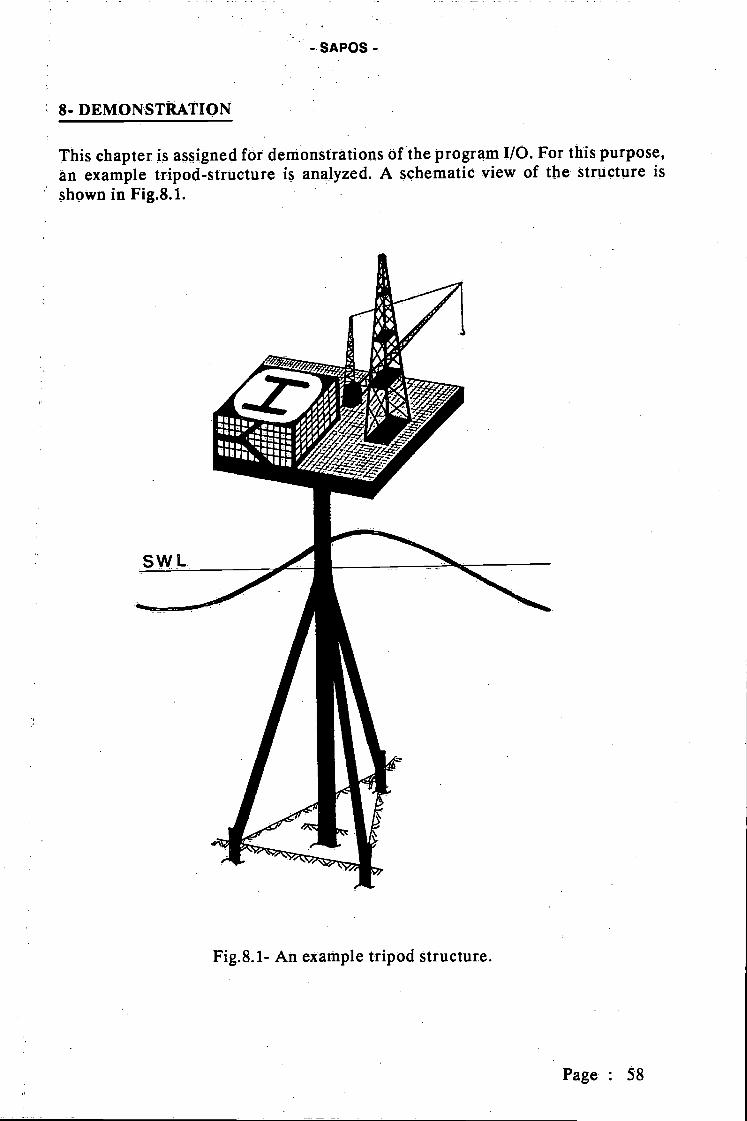
-. SAPOS -
8- DEMONSTRATIQN
This chapter is assigned fr demonstrations óf the program I/O. For this purpose,an example tripod-structure is analyzed A schematic view of the structure isshown in Fig.8.1.
Fig.8.1- An example tripod structure.
Page : 58

- SAPOS -
As it is seen from the figure the structure cOnsists of one central column andthree inclined legs. For the demonstration purposes, the following data are used:
- The topside is 20 m. above the still water level,- The mean water-depth is 50 rn.,- The diameter of the column is 3 m.,- The legs have a diameter of 2 m.,- All wall thicknesses are 100 mm.,- The mass of the deck is 3000 ton,- The added mass coefficient is 0.9,- Marine growth thicknesses on members are 250 mm.
Further, it is assumed that all members are full of water up to the still water level,the column and the legs are clamped at the base since this example is only for thedemonstration of I/O For this reason, a very simple calculation model, shown inFig.8.2, is used.
Fig.8.2- A simple calculation model of the example structure.
Eigenvalue solution of this example is carried out using Delft University ofTechnology (DUT) version of ICES/STRUDL, see Ref [16] The first two lowestnatural frequencies are found to be w1=w2 2.11 rad/sec which correspond toidentical mode-shapes in orthogonal directions. These mode-shapes are obtainedto be flexural. The indirect inputs generated by STRUDL is presented in Tab.8.1
Page : 59
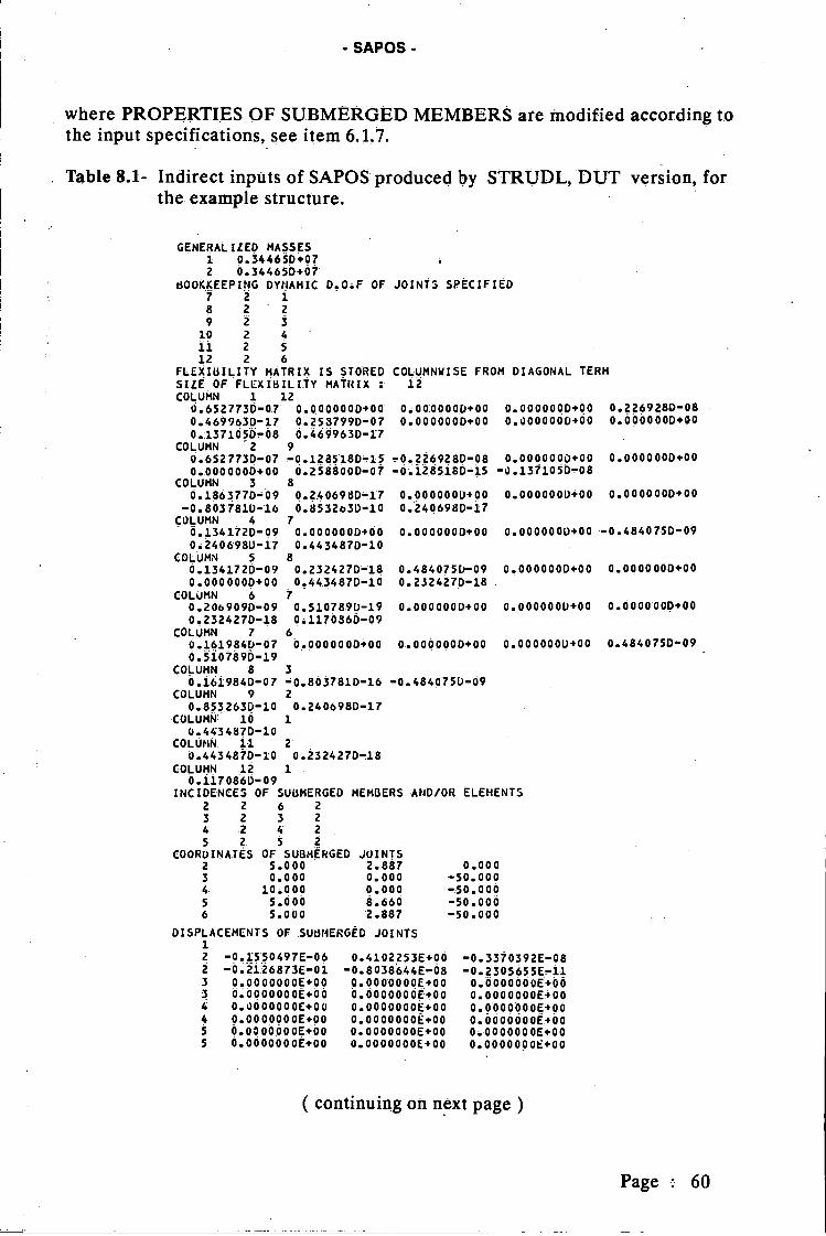
- SAPOS -
where PROPERTIES OF SUBMERGED MEMBERS are modified according tothe input specifications, see item 6.1.7.
Table 8.1- Indirect inputs of SAPOS produced by STRUDL, DUT version, fOrthe example structure.
GENERAL ¡LEO MASSES1 0.34465P+O?2 0.344650+07
BOOKKEEPING DYNAMIC7 2 18 229 2 3
10 2 4
11 2 5
12 2 6FLEXIBILITY MATRIX IS STORED
DoOoF OF JOINTS SPECIFIED
COLUMNWISE FROM DIAGONAL TERM
(continuing on next page)
Page 60
SIZE OF FLEXIBILITY MATRIXCOLUMN i 12
12
0.6527730-07 0.0000000+00 0.0000000+00 0.0000000+00 0.2269280-080.4699o3D-17 0.2587990-07 0.0000000+00 0.0000000+00 0. Ö 000 0 OD +00
0.1371050-08 0.4699630-17COLUMN 2 9
O.652773D-07 -0.1285180-15 -0.??4928P-08 0.0000000+00 0. 00 00 000+00
0.0000000+00 0.2588000-0? -0.1285180-15 -0.1311050-08COLUMN 3 8
0.1863?7Da09 0.240698D-17 0.00 0 00 0 0+ 00 o.0000000+00 0.000000D+00-0.8037810-16 0.8532b30-10 O. 2406980-17
COLUMN 4 7- 0.1341720-09 0.0000000+00 0.0000000+00 0.0000000+00 -0.4840750-09
0.2406980-17 0.4434870-10COLUMN 5 8
O.1341?2D-09 0.2324270-18 0.4840751)-09 0.0000000+00 0.000000D+000.0000000+00 0.4434870-10 0.2324270-18
COLUMN 6 70.ZOo909D-09 0.5107890-19 0. 000 00 00+ 00 0.0000000+00 0.0000000+000.232427018 0a117086D09
COLUMN 7 60.1619861)-07 0.0000000+00 0.0000000+00 0.0000000+00 0.4840750090.5107890-19
COLUMN 8 3
0.1619840-07 0.8037810-16 -0.4840751)-09COLUMN 9 2
0.8532630-10 0.2406980-17COLUMN 10 1
0.4434870-10COLUNÑ 11 2
0.44348?D-I0 0.2324270-18COLUMN 12 1
DISPLACEMENTS OF SUBMERGED JOINTS12 -0.1550497E-06 0.4102253E+00 -0.3370392E-082 -0.2126873E-01 -0.8038644E-08 -0.2305655E-ii3 0.0000000E+O0 0.0000000E+00 0.0000000E+003 0.0000000E+00 0.0000000E+00 0. 0 00 000 OE+006 0.0000000E+OO 0.0000000E+00 0.0000000E+004 O.0000000E+00 0.0000000E+00 0.0000000C+0O5 0.0300000E+00 0.0000000E+00 Oa 0000000E+005 0.0000000E+00 0.0000000E+00 0. 00000Oo+O0
0.1170860-09INCIDENCES OF SUBMERGED MEMBERS AND/OR ELEMENTS
2 2 6 2
3 2 3 2
4 2 4 2
5 2 5 2
COORDINATES OF SUBMERGED JOINTS2 5.000 2.887 0.0003 0.000 0.000 -50.0004 10.000 0.000 -50. 0095 5.000 8.660 -50.0006 5.000 2.887 -50.000
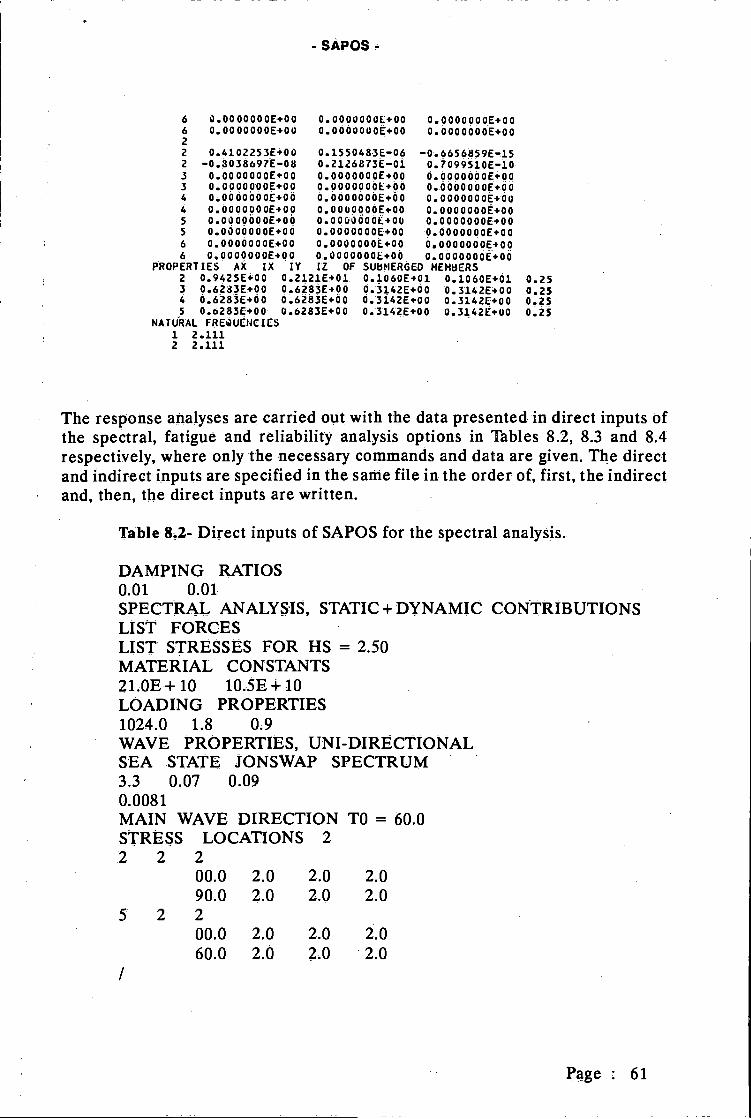
- SAPOS
PROPERTIES AX IX ¡Y IL 0F SUBMERGED H
1 2.1112 2.111
The response analyses are carried out with the data. presented in direct inputs ofthe spectral, fatigue and reliability analysis options in Tables 8.2, 8.3 and 8.4respectively, where only the necessary commands and data are given. The directand indirect inputs are specified in the same file in the order of, first, the indirectand, then, the direct inputs are written.
Table 8.2- Direct inputs of SAPOS for the spectral analysis.
DAMPING RATIOS0.01 0.01.SPECTRAL ANALYSIS, STATIC + DYNAMIC CONTRIBUTIONSLIST FORCESLIST STRESSES FOR HS = 250MATERIAL CONSTANTS21.OE+10 10.5E+iOLOADING PROPERTIES1024.0 1.8 0.9WAVE PROPERTIES, UNI-DIRECTIONALSEA STATE 3ONSWAP SPECTRUM3.3 0.07 0.090.0081MAIN WAVE DIRECTION TO = 60.0STRESS LOCATIONS 22 2 2
00.0 2.0 2.0 2.090.0 2.0 2M 2.0
5 .2 200.0 2.0 2.0 2.060.0 2.0 .0 2.0
/
Page : 61
E MB CR S
6 O.0000000E.00 O.0000000L+O0 o 0000000E. 006 O.0000000E.00 O.0000000E.00 0. 0000000E+O02
2 0.4102253E+Oi) 0.1550483E-06 -0.6656859E-152 -0.8038697E-08 0.2126873E-01 0.7099510E-103 O.0000000E.00 0.0000000E.00 o 0000000E. 003 O.0000000E+O0 0.0000000E+00 o. 00000ó OE.004 Ò.00Ö0000E+OÔ 0.0000000E+00 0. 000000 OEf 004 0.0000000E+00 0.0000000E+OO o. 0000 00 OÉ+ooS O.0000000E+ÓQ O.000000ÒE+O0 0. 000 000 0 E+OO5 0.0000000E+00 0.0000000E+0o 0. 000000 0 E+oo6 0,0000000E+00 0.0000000E+0O 0. 0 00 000 OE+006 0.0000000E+O0 0.0000000E+00 0. 000000 OE+OO
Z O.9425E+00 0.2121E+01, 0.1060E.01 0. 10 60 E+ 01 0.253 0 6283E+00 O 6283E+00 0.3142E+00 0. 314 2E. 00 0.254 0.6283E+O0 0.6283E+00 O.3142E+00 0. 314 ZE+00 0.255 0.6283E+00 0.6283E+00 0.3162E+0O U. 314 ZE+U0 0.25
NATURAL FREUENCICS
- SAPOS -
Table 8.3- Direct inputs of SAPOS for the fatigue analysis.
DAMPING RATIOS0.01 0.01FATIGUE ANALYSIS, STATIC+DYNAMIC CONT, ONE S-N LINE96.053 4.38 0.00 1.0LIST SPECTRAL MOMENTSMATERIAL CONSTANTS21.OE+10 10.5E+10LOADING PROPERTIES1024.0 1.8 0.9WAVE PROPERTIES, UNI-DIRECTIONALSEA STATE JONSWAP SPECTRUM3.3 0.07 0.090.0081 5WEIBULL DÏSTRBUTION FOR HS0.60 1.67 1.20MAIN WAVE DIRECTION TO = 60.0GAUSS POINTS FOR. FREQUENCY INTEGRATION 3
Table 8.4- Direct inputs of SAPOS for the reliability analysis.
DAMPING RATIOS0.01 0.01
RELIABILITY ANALYSIS, STATIC + DYNAMIC CONT, ONE S-N LINE96,053 438 0.00 1.0
LIFE TIME 25.0DESIGN VARIABLES
ITERATION NUMBER 2STIFFNESS MATRIX 0.04 NMASS MATRIX 0.08 NDAMPING RATÏOS 0.20 LMARINE GROWTHS 0.20 LALFA (SEA SPECT.) 0.15 NÖAMMA (SEA SPECT) 0.25 NINERTIA FORCES 0.20 L
(côntinuing on next page)
Page : 62
STRESS LOCATIONS 2
2 2 200.0 2.0 2.0 2.090.0 2.0 2.0 2.0
2 200.0 2.0 2.0 2.060.0 .0 2.0 2.0

SAPOS -
0.000.960.97
The outputs of SAPOS are demonstrated in the following pages throughoutTables 8.5 8.10.
Page 63
DRAG FORCES 0.20STRESS CONT. FAC. 0.12FATIGUE PARAMETERS
LNC1 0.024Kl 0.026 N
DAMAGE CORR. FAC. 0.30 LREFERENCE DAMAGE 0.25 NCORRELATION COEFFICIENTS
RO STIFFNESS AND MASSRO ALFA AND GAMMA (SEA SPECTRUMRO LNC1 AND Kl
/ END OF DESIGN VARIABLES ÏNPUTLIST SPECTRAL MOMENTSMATERIAL CONSTANTS21.OE±10 1O.5E+10LOADING PROPERTIES1024.0 1.8 0.9WAVE PROPERTIES, UNI-DIRETIONALSEA STATE JONSWAP SPECTRUM3.3 0,07 0.090.0Ù81 5WEIBULL DISTRIBUTION FOR HS0.60 1.67 1.20MAIN WAVE DIRECTION TO = 60.0GAUSS POINTS FOR FREQUENCY INTEGRATION 3
STRESS LOCATIONS 22 2200.0 2.0 2.0 2.090.0 2M 2.0 2.05 2200.0 2.0 2.0 2.060.0 2.0 2.0 2.0
/

1 0.12002 0.17523 0.27774 0.46925 0.59726 0.72527 0.85328 19449 1.5944
iO 1.8944Ii. 2.019412 2.095313 2.126714 2.176715 2.251716 2.401717 2.701718 3.101719 3.701720 4.601721 5.801722 6.3330
N.6. : THESE FREQUENCY BLOCKS CORRESPOND TO THE FIRST ITERATIONWHEN THE RELIA5ILITY ANALYSIS IS CARRIED OUT.
- SAPOS
Table 8.5- Output of frequency b1oks
S SSSS SSSS S SS SSS SSSSSS SS SSSSSS SS SS SS
O A
O A
O STOCHASTIC ANALYSIS PROGRAM A
O FOR ÓFFSHORE STRUCTURES A
O SAPOS VERSION 3 - A
O RELEASED BY DUT CAPRIL,198&) A
O A
O /OUTPUT/ A
O A
O AppppppppppppppppppPPPPpppPPPPPPPPPP
FREQUENCY 3LOCKS
NO FREQUENCY
Page 64
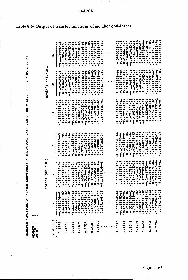
TRANSFER FUNCTIONS OF MEMBER END-FORCES / INDIVIDUAL WAVE DIRECTIOU = 60.000 DEG..
/lIS = 2.500
MEMBER :
2
JOINT
:2
FORCES (REa/IM.)
MOMENTS cRE./IM.)
F E U E NC Y
FX
FY
Fi
MX
MY
Mi
u) o u)
0.1274
-0. 4
71807E+0'2
-0. 163651'E+04
o .944338E+03
-0.196698E+0'l.
-0. 1
0 80 19 E+05
-O.18'7099E+O.5'
0. 42 1110 E+ 02
-0 .301617E+04
O174150E + 04
O1863S7E+
0.0
-0.1
03045E+05
-0. 1.78'521E+05
0.1.502
-0.6
4 49 43 E+ 02
-O1942 52 E.+04
0.11215 1E+04
-0 .230336E+01
-0 .126?69E+O5
-0.2
19 57 8E+05
0. 4960 08'E+ 02
-0 .415383E+04
O 2'39335E+04
O.274510E+00
-0.140 671E+05
-0.243697E+05
0.1699
-0. 8
127 48E'+ 02
-0..221630E+04
0. 12 795 8E+O4
-0.2590'15E+01.
-0.142914E+05
-O .247542E+05
0.561278E+02
-O.527323E+04
O.304466E+04
o .377195'E+00
-0. 17 70 20 E+05
-O.3
066 61E+05
0.1895
-0. 9
94604E+02
-O24994.2E+04
o .144302E+04
-0.286653E+01
-O. 1
5:8921E+ 05
-0. 27 527 OE+05
0.626842E+02
-06 505 9.4 E+,O.4
0. 37 5639 E+04
0.511732E+0O
-0216265E+0.5
-O .3 74 64 3E+05
0.2 322
-0.1
429 62 E+ 03
-0315904E+04
0'.1
82 38 3E
+06
-0'.344147E+01
-0.1.933'80E+05
-Q .334966E+'05
0.771472E+02
-095 4 467E +04
0.551084E+04
O.974639E+00
-0.309393.E+05
-O 53595 8E.+05
o 2681
-0. 182768E+03
-O
3.77953E + 04
O .218202E+04
-O.3'87703E+01
-02'22251E+05
-O.384985E+05
0.897086E+02
-0.124505E+05
O.718856E+04
0.164979E+0]..
-0.3
9 3630 E+05
-0.6
81524E+05
0.305.3
-0. 225649E+O3
-3.4
5'0338E+04
0.2 5 998 8E +04
-O.426600E+0i.
-0. 2
5 2022E+05
-0.
. 4 36 57 6E+.O 5
0'.103180E+03
-0.157391E+05
0.908726E+04
o .277863E+01
-0.482260E+05
-0 835 38 OE+ 05
4.5092
O507634E+02
0. 606 8.29 E+04
-035
036 5E +04
-0.12247 9E'+ 02
0. 1785 93 E+06
0'..309332E+06
-0.103838E+03
0.2432'29E'+04
-0 .140403E+04
-0.61i.262E+01
0.858146E+05
O.148619EI06
4.7521
-0.647125'E+02,
-0.7
5 17 70 E+ 02
O .405710E+04
-0.409215E+04
-0.234223E+04
O236279E+04
-O .7'99432E+01
0.675.293E+01
Ô. 12 4636 E+06
-0. 10 9 072 E+ 06
O .,215862E+06
-0 .188923E+06
5.2361
0. 5 538 53E+ 03.
-0 .447572E+04
0.25 8'612E+04
O .679614E'+Ol
-O .119684E+Oo
-0.20 7298E+06
0. 7470 95 E+ 02
0. 744137E+03
-0 .429602E+03
-0 .42923IE+00
0. 10 16 61E+05
O. 17617 1EO 5
5.6 7.91
0. 3166 44E+02
O 332347E+04
-O .191896E+04
0 .368452E+0].
0..? 89114 E+05
O .136689E+O.6
-0. 501408E+02
0.i.65562E+04
-0 .955856E+O3
-0 .2 3959 8E+ 01
O.484054E+Q'5
33 841.8 E+05
5. 8639
-0. 2.789 84E+02
o Z?3?92E+04
-O .158076E+04
-0 .315126E+01
0..711428E+05
O.123220E+06
-0. 463 867E+02
-0..206837E+.04
O - 11942 7E +04
o .183360E+0'l
-0 .441664E+05
-O .764994E+05
6.0 731
-O. 4732'33E+02
-0 .11 50 07E+0.4
O 664081E + 03'
o .7812.38E+0.0
-0. 206732E+O5
-0. 35'8126E+05
0. 127980 E+02
-0.293142E+04
O .169246E+06
o .307619E+01
-0 .722482E+05
-0.12 5139E+06
6.2754
-0. 6470 36E+00
-0.289291E+06
o .16?034E+04
0. 2 3733 2E+ 0 3.
-0.680231E+05
-O .117820E+06
0. 4471?2E+02
0.2.90967E+03
-0.1680 33E+0'3
'0.776927E-01
0. 102665E+03
O..179535E+03

00 o o -t C'I
(D -t
0. 3855
0. 359970E+06
0. 20 78 56 E+06
0 6.517
0. 423 350 E+06
0.24 4 4 45 E+0 6
(D
0.4853
0. 44 813:7E+ 06
0. 258751E+06
o.0.5.370
0.473912 E+06
0.. 2.73 625E+0.6
0.5842
0.6130
0.6643
0. 482624E+06
0. 480418E+06
0.461492 E+06
0.2 78 65 2 E+0 6
0. 277 374E+06
0. 2 6.64 47E +06
Cd, o.
0.7119
O. 426134È+06
0. 246 03.7E+O:6
(D0.7407
O. 396290E+06.
o .2288,04E+0.6
0.7918
0. 32.7 547E+O6
0.189133E+0.6
0.8397
O. 244448E+06
0.1,4117.2E+O,r6
(D -to.;898i.
0. 118894E+06
0..687530E+0 5
(D cd,
-Cd, (D
3.813.7
0. 176668E+07
0:. 101999E+Ø7
Cd,
4.1760
0.127126E+07
o .733.966E+06
4.. 5092
0. 971125 E+06
0. 560694E+06
4.7521
0. 811746È+06
O.4686,75E+06
5.2361
0. 588719E+06
o .339899E+06
5.6,791
0. 4 537 62 E+ 06
0.261967E+0'6
5.8639
0. 410415E+06
O 23 6.9 5 9E +0.6
6.0731
0. 368329E+06
0.212652E+Ó.6
6. Z7 54
0.333401E106
0. 192 491E +0 6
O 1274
0.731681E+05
0422557E+05
0.1502
0. 928112E+.05
0. 535993E+05
0.
1699
0.1i1507E+0.6
0. 643959E+05
0 .1895
0.. 131538E+06
0.759627E+05
0.2322
O .1788 26 E+ 0,6
0. 1032 68E+06
0.2681
0. 221474E+06
0.12 7893E+06
0.3053
0.2667 OIE+06
0.Ï54008E+06
MODULUS OF HOT-SPOT NORMAL-STRESS TRANSFER; FUNCTIONS / IND:IVIDUAL WAVE DIRECTION= 60.000 DEG. /
liS = 2.500
MEMER :
2
JOINT
Z
FREQUENCY
ALFA
0..0
ALFA
9.0.0

C.
00 00 o o ri,
(D '-1 o (D rl) o o rl) o ri 1 (D Cl)
CI) (D Cl)
22
0.0
2.00
002_
0100
02.
0000
1.15
0O
.360
6E+
.14
0. 1
598E
+1
5O
.7 1
4 3E
+ 1
52
20.
02.
00.0
02.
00:0
0.2.
0000
2.82
8O
4 2
29E
+14
O.1
868E
+15
o .8
332E
+15
2 2 2
2 2 2
0.0
O..O
0.:0
2.00
002.
0000
2.00
00
2.00
002.
0.00
02.
0.00
0
2.00
002.
0000
2.00
00
5.45
29.
Ï38
14.4
31
0.43
84E
+14
0'. 4
529.
E+
14'0
.796
'E+
14
0. 1
92 I
E+
150.
194
8E
+15
0. 1
97 5
E+
15
0.85
62E
+1.
.50.
867
1E+
1'5
0. 8
.779
E.+
15.
2 2 2 2 2
2 2 2 2 2
90.0
90.0
90.0
90.0
90.0
2.00
002.
0000
2.00
002.
0000
2.00
00
2.0.
000
2.00
002:
.000
02.
0000
2.00
00
2.00
.00
2.00
0Ó2.
00:0
02.
0:00
02.
00.0
0
1.15
02.
828
5.45
29.
138
14.4
31,
0._1
202
E+
14O
141
0E +
140.
1461
E+
140
..1 5
10 E
+14
0 .1
599E
+14
0.. 5
3 2
5E +
140.
6226
E+
140.
640
5 E
+14
0.. 6
4.93
E +
140.
6584
E+
14
.0. 2
38
liE +
150.
27
7 7E
+15
0.. 2
85 4
E+
150.
2890
E+
150.
2.9
26E
+15
5a
52
52
S2
52
0.0
0.0
0.0
0.0
0.0
2.00
0:0
2.00
002.
00oO
2.03
002.
00:0
0
2.09
002.
0000
2.00
002.
0000
2.00
00
2.00
:0,0
2.00
002.
0:00
02.
0.00
02.
0000
1.15
02.
828
5.45
29.
138
14.4
31
0. 9
294
E+
140.
1215
E+
150
.143
6E+
150.
.171
6E+
150.
2 16
6E+
15
0. 3
94 4
E+
1.5
0:.,4
,7 3
:2 E
+15
O 4
9.5
6E+
1 S
0.50
97E
+1.
50.
5 24
5E
+15
0. 1
7 17
E+
16
Ô..
2:O
j.E+
jØ
: 208
5E+
160.
2115
E+
16O
..21
44E
+16
5 5 5 5 5
2 2 2 2 2
60.0
60.0
60.0
60.0
.60
.0
2.00
002.
0000
2.00
002.
00.0
.02.
0000
2.00
002.
0000
2.00
002.
0000
2.00
0.0
2.00
002.
0000
2.00
GO
2.00
002.
00:0
0
1.j.5
O2.
828
5.4.
5:2
.9.
138
14.4
31
O .3
213E
+14
0.4
625E
+14
O .6
035E
+14
0.7
861E
+14
0.10
73E
+15
OE
.131
8E+
15O
.162
1E+
15O
. 17
2:8E
415
0.18
02E
+.1
5.0.
.187
9E+
1 5
0.56
29E
+15
0..6
.675
E+
150.
690
7E
+15
o .7
0ZO
E+
1,5
0.71
2 6E
+1
5
SPE
CT
RA
L M
OM
EN
TS
OF
rIO
T-S
POT
NO
RM
AL
ST
RE
SSE
S / I
ND
Iv,I
:DuA
L W
AV
E D
IRE
CT
ION
= 6
0.00
.0 D
EG
o
ME
MB
ER
JOIN
TA
LFA
S.C
FCN
)SC
F(M
Y)
.SC
F(M
i)H
SM
OM
2M
4
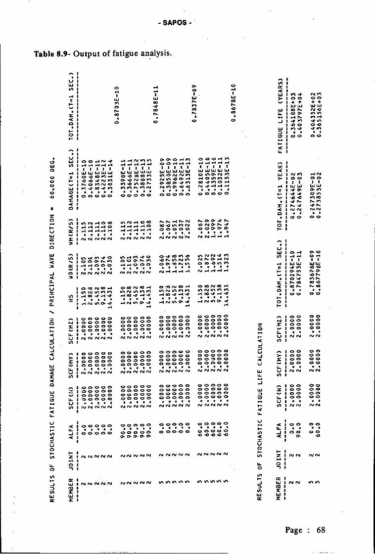
RESULTS OF STOCHASTIC FATIGUE DAMAGE CALCULATION I PRINCIPAL WAVE DIRECTION =
60.000 DEG.
MEM8ER.
JOINT
ALFA
SCF(N)
SCFCMY)
SCFCMZ)
HS
¿2
0.0
2.0000
2.0000
2.0000
1.150
2.105
2.115
22
0.0
2.0000
2.000.0
2.0000
2.828
2.101
2.112
22
0.0
2.0000
2.0000
2.0000
5.652
2.093
2,111
22
0.0
2.0000
2.0000
2.0000
9.138
2.074
2.110
22
0.0
2.0000
2.0000
2.0000
14.431
2.030
2.108
22
90.0
2.0000
2.0000
2.0000
1.1.50
2.105
2.115
22
90.0
2.0000
2.0000
2.0000
2.828
2.101
2.112
22
90.0
2.0000
2.0000
2.0000
5.452
2.093
2.111
22
90.0
2.0000
2.0000
2.0000
9.138
2.074
2.110
22
90.0
2.0000
2.0000
2.0000
14.431
2.030
2.108
52
0..0
2.0000
2.0000
2.0000
1.150
2.060
2.087
52
0.0
2,0000
2.0000
2.0000
2.828
1.974
2.067
52
0.0
2.0000
2.0000
2.0000
5.452
1.858
2.051
52
0..0
2.0000
2.0000
2.0000
9.138
1.723
2.037
52
0.0
2.0000
2.0000
2.0000
14.431
1.556
2.022
52
60.0
2.0000
2.0000
2.0000
1.150
2.025
2.067
52
60.0
2.0000
2.0000
2.0000
2.828
1.872
2.0:29
52
60.0
2.000.0
2.0000
2.0000
5.452
1.692
1.999
52
60.0
2.0000
2.0000
2.0000
9.138
1.514 .
1.974
52
60.0
2.0300
2.000.0
2.0000
14.431
1.323
1.947
WO(R/S)
WM(R/S)
DAMAGE(T=1 SEC.)
TOT.DA'M.(T=I SEC.)
0.3760E-1,0
0.4066E-10
0.8368E-11
0.4223E-12
0.3 031E-14
O .3390E-il
0.3666E-11
0.7528E-12
0.3808E-13
0.2733E-15
0.2925E_09
0.3850E-09
0.9962E-10
0.6492E-11
0.6313E-13
o .2810E-10
0.4405E-10
0.1359E-10
0.1032E-11
0.115,3E-13
0.8703E-10
0.7848E-11
O .7837E-09
0.8678E-10
TOT.DAM.CT=j. YEAR)
FATIGUE LIFE (YEARS)
0.274644E-02
0.. 364108E + 03
0.247649E-03
O 4 037 97E +04
0.247309E-03.
0.40.4352E+02
0.273855E-02
0.365156E+03
RESULTS OF STOCHASTIC FATIGUE LIFE CALCULATION
MEMßER
JOINT
ALFA
SCFCN)
'SCF(MY)
SCF(MZ)
TOT.DAM.C'T=l SEC.)
22
0'..O
2.0000
2.0000
2.00.00
0.870.294E-10
22
90.0
2.0000
2.0000
2.0000
0.786753E-11
52
0.0
2.0000
2.0.000
2.0000
0.783676E-09
52
60.0
2.0000
2.0000
2,0000
0.867796E-10

RESULTS OF FATIGUE RELIABILITY CALCULATION (ITERATION NO':
2)
aSTIFFNESS AND M'SS MATRICES.*
*....(UNCORRELATED PAIR)
*-DAMPING RATIOS
-THICKNESS OF MARINE GROWTHS
*ALF
A A
ND
GA
MM
A. J
OP
IS.W
AP
SE
A*
*SP
EC
TR
UM
,(iJ
NC
OR
RE
LAT
ED
PA
IR.)
*-I
NE
RT
IA F
OR
CE
CO
EF
FIC
IEN
T-DRAG FORCE COEFFIC.IENT.a...,u
-STRESS CONCENTRATION FACTORS
*PARAÑETÈRS UF THE S-H LI.NE...*
a..... CUÑCORRELAÏED PAIR)
.. ...
*-DAMAGE CORRECTION FACTOR
-REFERENCE DAMAGE TO FAILURE
N.B.
:IN THIS LIST STATI:STICAL VALUES CORRESPOND TO THE EQUIVALENT NORMAL OISTRIBUTION.
(con
tinui
ng o
n ne
xt p
age)
0.40
00E
-01
O ..8737E+01
0. 25 26E. 00
O .0
.638
30.9960'OE+'0O
0.8000E-01.
- .3909E+01.
-.22
61E
+O
00.05110
0. 1
0 07
2E
+01
O ..l937E+0O
0.2036E+0].
0.27
96E
+00
0.07
817
O .9
5931
.E+
00O
20 09E
+ 0
0-.
1312
E+
Oi.
-.,1
868E
+00
0. 03 489
0.99505E+O0
-.2500E+00
o.2
969E
+00
0.17
71'
E+
0 O
0.03
135
-..33579E+01
-.1167E00
o.2
304E
,+03
0.70
45E
-01
0.0
0496
-.36366E-02
0.2078E+00
-.41
81E
,+01
.-.
.615
3E+
000.
3.7
856
0. 102 91E+01
0.0000E+0O
-.33
53E
-01
0.0000E+00
0.00000
0. 10 00 OE+01
0. 12 00 E +0 0
-.42
5.5E
+01
-.3691E+O0
0..1
362.
70.
.101
75'E
+01
-.2400E-01
-.14
68E
+00
-.2449E+00
0,. 0.5996
-.95
929E
+02
-.1241E+00
-.1
.78
3E+
0:2
-.35
65E
+0O
0.12
7 06
-.2Ï
9.O
IE+
O0
0. 300 OE+ 00
o.3
966E
-01.
0.00
00E
+00
O .000 0:0
0. 000 OOE+00
0..2
5:0
0 E
+00
O .1
018E
+01
0.18
4 0.
E+
000.03386
0.98
179E
+00
MEMBER
:5
JOINT
2ALFA
0.,0
TOTAL FATIGUE DAMAGE
(1=
1. S
EC
...)
:0.
.124
141E
-08
FAILURE FUÑCT. (1= 25.00 YEARS)
:0.31070IE-02
MEAN OF FAILURE FUNCTION :
O.54772.OE+O0
STAND.DEV. 0E FÀIL,.FUNC.
:0.138322E+O1
RELIABILITY INDEX (BETA)
:O.395975E+0O
DESIGNATION OF VARIABLES
NO
ME
AN
VA
LUE
VAR.COEFF.
DERIVATIVE
SENS. FACT.
CONTRIBUT ION
DE
SIG
N P
O:IN
T
Xl
0.l00:OE+01
0. io o
ox
X3
0.98 03 E+0O
X'
0. 9 805E
'O O
X5
-.33OOE+Oi
X6
-.3625E-02
X 7
0..9
795 E+ O O
X8
0.I000E+O1
X9
0.10
OO
E+
O1
X10
-.9615E+02
Xli.
-.2229E+00
X14
O 0
0 00
E+
0.0
X15
0. 1
00,O
E+
01

SUMMARY OF THE FAT1GUE RELIABILITY CALCULATION FOR
125.00 YEARS
(ITERATION NO: 2
)
MEMBER
JOINT
ALFA
FAIL.F.UNC.
22
0.0
22
90.0
52
0'.o
52
60..O
O .2 17 8E+ 01
0.45 8.OE+01
0.3107E-02,
0..2216E0i
Z MEAN
0.2739E+Oi.
0.;5145E+01
0. 547 7E+O0
0.27 53E+O1
STAND.. DEy.
0.,1425E+01
0. 14 38E.+ 0].
0.138 3E+ 01
0,. 136 9.E+01
REL. INDEX
0. 19 22 E+ 01
0. 35 78E+ 01
0. 39 60E+00
0.201 IE+ 01
N.B.
CALCULATION
ILL BE RESUMED WITH NEW DESIGN VALUES ASSOCiATED WITH
THE STUESS POI WT Ai1D THE MINIMUM RELIABILITY IÍNDEX
(BETA),
MEIIBER
:5
JOINT
:2.
'ALFA
:0..00
BETA
:0.396
- SAPOS -
REFERENCES
[1] Karadeniz, H., Stochastic Analysis Program for Offshore Structures(SAPOS), Report, Dept. of Civil Engg., Delft University of Technology,Delft, May, 1985.Karadeniz, H., et al. "Probabilistic Reliability Analysis for the Fatigue limitstate of Gravity and Jacket-type Structures", Third InternationalConference on Behaviour of Offshore Structures, BOSS'82, Vol.2,pp.147-165, Hemisphere Pub. Corporation, New York, 1983.Cloiigh, R.W. and Penzien, J., Dynamics of Structures, McGraw- Hill, 1975.Karadeniz, H., Spectral analysis and stochastic fatigue reliability calculationof offshore steel structures, Report, Dept. of Civil Engg., Deift UniversityofTechnology, Deift, April, 1983.Vugts, S. H. and Hines, I. M. "Modal Superposition y Direct SolutionTechnique in the dynamic analysis of Offshore Structures", SecondInternational Conference on Behaviour of Offshore Structures, BOSS'79,London, 1979.Karadeniz, H. "An implicit calculation procedure for spectral responsestresses in offshore structural members", Proceedings of the Eighth JointInternational Conference on Offshore Mechanics and Polar Engineering(OMAE), The Hague, The Netherlands, March 19-23,1989.Karadeniz, H., An integration procedure to calculate response spectralmoments of offshore structures, Report, Dept. of Civil Engg., DeiftUniversity of Technology, Deift, April, 1980.Karadeniz, H., Probabilistic Fatigue Damage calculation of Offshorestructures under narrow- and broad-band stress processes, Report, Dept. ofCivil Engg., Delft University of Technology, Deift, October, 1987.Abramowitz, M. and Stegun, I. A., Handbook of Mathematical Functions,Dover Publications Inc., Academic Press, New York, 1972.
[101 Brebbia, C.A. and Walker, S., Dynamic Analysis of Offshore Structures,Butterworth & Co. (Publishers) Ltd., London, 1979.Thoft-Christensen, P. and Baker, M.J., Structural Reliability Theory and ItsApplications, Springer-Verlag, Berlin,1982.Madsen, H.O., Krenk, S. and Lind, N. C., Methods of Structural Safety,Prentice Hall Inc., Englewood Cliffs, 1986.Hallam, M.G., Heaf, N.J. and Wooton, L.R., Rationalisation of Safety andServiceability Factors in Structural Codes, CIRIA, Report No.63, 6 Storey'sGate, London, 1976.Hohenbichler, M. and Rackwitz, R. "Non-Normal Dependent Vectors inStructural Safety", Journal of the Engineering Mechanics Division, ASCE,Vol.107, pp.1227-1238, 1981.Rackwitz, R. and Fiessler, B. "Structural Reliability under CombinedRandom Load Sequences", Computers and Structures, Vol.9, pp.484-494.,1978.Kok,A.W.M., Vrijman, C.F. and Boer, A., ICES I STRUDL Users Manual,Part i and 3, Calculation of Framework and Dynamic Analysis, Report,Dept. of Civil Engg., Deift University of Technology, Delft, October, 1984.
Page 71