advanced research version of the weather research and ...(wrf-arw), with atmospheric observations....
TRANSCRIPT

ARL-TR-8803 ● SEP 2019
Advanced Research Version of the Weather Research and Forecasting (WRF-ARW) Model Runs at Jornada Experimental Range by Jeffrey E Passner Approved for public release; distribution is unlimited.

NOTICES
Disclaimers
The findings in this report are not to be construed as an official Department of the Army position unless so designated by other authorized documents. Citation of manufacturer’s or trade names does not constitute an official endorsement or approval of the use thereof. Destroy this report when it is no longer needed. Do not return it to the originator.
ARL-TR-8803 ● SEP 2019
Advanced Research Version of the Weather Research and Forecasting (WRF-ARW) Model Runs at Jornada Experimental Range Jeffrey E Passner Computational and Information Sciences Directorate, CCDC Army Research Laboratory
Approved for public release; distribution is unlimited.

ii
REPORT DOCUMENTATION PAGE Form Approved OMB No. 0704-0188
Public reporting burden for this collection of information is estimated to average 1 hour per response, including the time for reviewing instructions, searching existing data sources, gathering and maintaining the data needed, and completing and reviewing the collection information. Send comments regarding this burden estimate or any other aspect of this collection of information, including suggestions for reducing the burden, to Department of Defense, Washington Headquarters Services, Directorate for Information Operations and Reports (0704-0188), 1215 Jefferson Davis Highway, Suite 1204, Arlington, VA 22202-4302. Respondents should be aware that notwithstanding any other provision of law, no person shall be subject to any penalty for failing to comply with a collection of information if it does not display a currently valid OMB control number. PLEASE DO NOT RETURN YOUR FORM TO THE ABOVE ADDRESS.
1. REPORT DATE (DD-MM-YYYY)
September 2019 2. REPORT TYPE
Technical Report 3. DATES COVERED (From - To)
January 2015–August 2019 4. TITLE AND SUBTITLE
Advanced Research Version of the Weather Research and Forecasting (WRF-ARW) Model Runs at Jornada Experimental Range
5a. CONTRACT NUMBER
5b. GRANT NUMBER
5c. PROGRAM ELEMENT NUMBER
6. AUTHOR(S)
Jeffrey E Passner 5d. PROJECT NUMBER
5e. TASK NUMBER
5f. WORK UNIT NUMBER
7. PERFORMING ORGANIZATION NAME(S) AND ADDRESS(ES)
CCDC Army Research Laboratory* ATTN: FCDD-RLC-EM White Sands Missile Range, NM 88002-5001
8. PERFORMING ORGANIZATION REPORT NUMBER
ARL-TR-8803
9. SPONSORING/MONITORING AGENCY NAME(S) AND ADDRESS(ES)
10. SPONSOR/MONITOR'S ACRONYM(S)
11. SPONSOR/MONITOR'S REPORT NUMBER(S)
12. DISTRIBUTION/AVAILABILITY STATEMENT
Approved for public release; distribution is unlimited. 13. SUPPLEMENTARY NOTES *As of February 2019, the US Army Research Laboratory has been renamed the US Army Combat Capabilities Development Command Army Research Laboratory (CCDC ARL). 14. ABSTRACT
The CCDC Army Research Laboratory (ARL) is interested in high spatial and temporal resolution weather output with an emphasis on products that assist Warfighter decision aids and applications in battlefield environments. A model study was performed in support of the short-range Army tactical analysis/nowcasting system called the Weather Running Estimate-Nowcast, as well as longer-range forecasting support. The model used to investigate fine-scale weather processes, the advanced research Weather Research and Forecasting model (WRF-ARW), was run with a triple nest of 9-, 3-, and 1-km grids over a 24-h period. One of the long-term intriguing areas of study is investigating model performance in complex terrain, such as the Jornada Experimental Range and White Sands Missile Range in New Mexico. Model performance and validation are highly dependent on available initial data and data input. In many areas, weather observations remain inadequate to optimally run and evaluate high-resolution models such as the WRF-ARW. ARL developed the Meteorological Sensor Array (MSA), an agile, finely spaced grid of surface meteorological sensors to assist atmospheric models. This report is focused on model runs in complex terrain and how the MSA can help improve data assimilation and model performance. 15. SUBJECT TERMS
mesoscale, weather research and forecasting model, WRF-ARW, wind, Jornada Experimental Range
16. SECURITY CLASSIFICATION OF: 17. LIMITATION OF ABSTRACT
UU
18. NUMBER OF PAGES
47
19a. NAME OF RESPONSIBLE PERSON
Jeffrey E Passner a. REPORT
Unclassified b. ABSTRACT
Unclassified
c. THIS PAGE
Unclassified
19b. TELEPHONE NUMBER (Include area code)
(575) 678-3193 Standard Form 298 (Rev. 8/98)
Prescribed by ANSI Std. Z39.18

iii
Contents
List of Figures iv
List of Tables v
1. Introduction 1
2. Weather Research and Forecasting (WRF) 1
3. Meteorological Sensor Array (MSA) 3
4. Fundamentals of Flow in Complex Terrain 7
5. Examples of Wind Flow at JER 9
5.1 12 Jan 2016: Light Wind Case 9
5.2 10 Apr 2019: Strong Wind Case 23
6. Discussion 29
7. Conclusion 36
8. References 37
List of Symbols, Abbreviations, and Acronyms 39
Distribution List 40
iv
List of Figures
Fig. 1 Three domains for the WRF model runs............................................... 2
Fig. 2 JER northeast of Las Cruces, New Mexico .......................................... 4
Fig. 3 Proposed and current locations of the MSA sensors at JER and WSMR............................................................................................ 5
Fig. 4 MSA Tower #4 at WSMR, New Mexico.............................................. 5
Fig. 5 10-m tower (Climatronics Corp 2014). Used with permission from David W Gilmore, Met One Instruments, Inc., Climatronics Division. 6
Fig. 6 General valley/slope flows during the night (left) and day (right) ....... 7
Fig. 7 500 hPa upper-air chart at 1200 UTC 12 Jan 2016 ............................. 10
Fig. 8 1200 UTC upper-air sounding at Santa Teresa, New Mexico, (EPZ) on 12 Jan 2016 .................................................................................... 10
Fig. 9 Surface weather chart at 1200 UTC (0600 local daylight time [LDT]) 12 Jan 2016 ......................................................................................... 11
Fig. 10 Surface winds and speeds (m/s) on at 1300 UTC 12 Jan 2016 ........... 12
Fig. 11 Surface temperatures (°C) at 1300 UTC 12 Jan 2016 ........................ 13
Fig. 12 Vertical temperature profile (°C) over JER headquarters at 1400 UTC 12 Jan 2016 ......................................................................................... 14
Fig. 13 Surface winds and speeds (m/s) at 1600 UTC 12 Jan 2016 ................ 15
Fig. 14 Vertical temperature profile (°C) over JER headquarters at 1600 UTC 12 Jan 2016 ......................................................................................... 16
Fig. 15 Surface winds and speeds (m/s) at 2100 UTC 12 Jan 2016 ................ 17
Fig. 16 Vertical temperature profile (°C) over JER headquarters at 2100 UTC 12 Jan 2016 ......................................................................................... 18
Fig. 17 Surface temperatures (°C) at 2200 UTC 12 Jan 2016 ........................ 19
Fig. 18 Surface temperatures (°C) at 0000 UTC 13 Jan 2016 ........................ 20
Fig. 19 Surface winds and speeds (m/s) at 0600 UTC 13 Jan 2016 ................ 20
Fig. 20 Surface winds and speeds (m/s) at 1100 UTC 13 Jan 2016 ................ 21
Fig. 21 Vertical temperature profile (°C) over JER headquarters at 1200 UTC 13 Jan 2016 ......................................................................................... 22
Fig. 22 500-hPa upper-air chart at 1200 UTC 10 Apr 2019 ........................... 24
Fig. 23 1200 UTC upper-air sounding at EPZ on 10 Apr 2019 ...................... 24
Fig. 24 Surface weather chart at 1200 UTC (0600 LDT) 10 Apr 2019 .......... 25
Fig. 25 Forecasted surface temperature and wind direction at 1200 UTC 10 Apr 2019 ............................................................................................. 26

v
Fig. 26 Forecasted low-level temperature profile (°C) at 1200 UTC 10 Apr 2019 ........................................................................................ 27
Fig. 27 Forecasted wind speed (m/s) and direction at 1400 UTC 10 Apr 2019............................................................................................................. 28
Fig. 28 Forecasted wind speed (m/s) and direction at 2100 UTC 10 Apr 2019............................................................................................................. 28
Fig. 29 Forecasted wind speed (m/s) and direction at 1200 UTC 11 Apr 2019............................................................................................................. 29
Fig. 30 Gap flows forecasted between the mountain peaks at 1300 UTC 9 Apr 2015 .......................................................................................... 30
Fig. 31 Forecasted transitional flow over JER at 1200 UTC 2 Nov 2015 ...... 31
Fig. 32 Weak drainage flow predicted on the west slope converges with down-valley flow over JER at 1300 UTC 28 Jan 2016 ...................... 31
Fig. 33 Forecasted temperatures (℃) for southern New Mexico at 1300 UTC 13 Oct 2015 ......................................................................................... 32
Fig. 34 Verified temperatures from 1300 UTC 13 Oct 2015 over southern New Mexico using https://mesowest.utah.edu ............................................ 32
Fig. 35 Forecasted wind flow over the JER area at 2300 UTC 25 Apr 2015 . 33
Fig. 36 Forecasted wind flow over the JER area at 1800 UTC 15 May 2015 34
Fig. 37 Flow over the JER area at 2300 UTC 12 Apr 2018 ............................ 35
Fig. 38 Forecasted flow over the JER at 0000 UTC 13 Apr 2018 .................. 35
List of Tables
Table 1 Sounding at 1200 UTC 13 Jan 2016 from surface to 700 hPa at Santa Teresa, New Mexico (EPZ) ................................................................ 23
1
1. Introduction
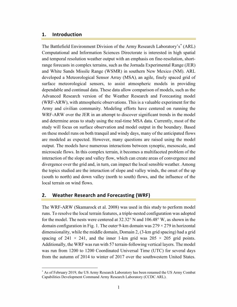
The Battlefield Environment Division of the Army Research Laboratory’s* (ARL) Computational and Information Sciences Directorate is interested in high spatial and temporal resolution weather output with an emphasis on fine-resolution, short-range forecasts in complex terrains, such as the Jornada Experimental Range (JER) and White Sands Missile Range (WSMR) in southern New Mexico (NM). ARL developed a Meteorological Sensor Array (MSA), an agile, finely spaced grid of surface meteorological sensors, to assist atmospheric models in providing dependable and continual data. These data allow comparison of models, such as the Advanced Research version of the Weather Research and Forecasting model (WRF-ARW), with atmospheric observations. This is a valuable experiment for the Army and civilian community. Modeling efforts have centered on running the WRF-ARW over the JER in an attempt to discover significant trends in the model and determine areas to study using the real-time MSA data. Currently, most of the study will focus on surface observation and model output in the boundary. Based on these model runs on both tranquil and windy days, many of the anticipated flows are modeled as expected. However, many questions are raised using the model output. The models have numerous interactions between synoptic, mesoscale, and microscale flows. In this complex terrain, it becomes a multifaceted problem of the interaction of the slope and valley flow, which can create areas of convergence and divergence over the grid and, in turn, can impact the local sensible weather. Among the topics studied are the interaction of slope and valley winds, the onset of the up (south to north) and down valley (north to south) flows, and the influence of the local terrain on wind flows.
2. Weather Research and Forecasting (WRF)
The WRF-ARW (Skamarock et al. 2008) was used in this study to perform model runs. To resolve the local terrain features, a triple-nested configuration was adopted for the model. The nests were centered at 32.32° N and 106.48° W, as shown in the domain configuration in Fig. 1. The outer 9-km domain was 279 × 279 in horizontal dimensionality, while the middle domain, Domain 2, (3-km grid spacing) had a grid spacing of 241 × 241, and the inner 1-km grid was 205 × 205 grid points. Additionally, the WRF was run with 57 terrain-following vertical layers. The model was run from 1200 to 1200 Coordinated Universal Time (UTC) for several days from the autumn of 2014 to winter of 2017 over the southwestern United States.
* As of February 2019, the US Army Research Laboratory has been renamed the US Army Combat Capabilities Development Command Army Research Laboratory (CCDC ARL).

2
The case days were selected to include days with “quiet” weather and days with synoptically dominated or more active weather. The observation nudging capability of WRF (Deng et al. 2009) is used to incorporate observations in some of the cases into the model via a preforecast (6 h starting at 0600 UTC); however, for this initial part of this study, using the southern New Mexico study area, the model was run without using observational nudging in the forecast on all but three of the days.
Fig. 1 Three domains for the WRF model runs
The North American Mesoscale Model (NAM) 12-km horizontal resolution output was used to create initial conditions and boundary conditions for the WRF, although some of the cases used Global Forecast System (GFS) data for initial and boundary conditions. The Mellor-Yamada-Janjić scheme (MYJ; Janjić 2001) was used to parameterize the atmospheric boundary layer (ABL). As in Lee et al. (2012), the background turbulent kinetic energy (TKE) is decreased to better simulate conditions with low TKE and the ABL-depth diagnosis is altered. In preliminary experiments for this study, the standard MYJ scheme resulted in noisy TKE fields and thus noisy ABL-depth fields over the water. These were resolved using the altered version of MYJ. The other parameterizations used included the Thompson microphysics parameterization, the Kain-Fritsch cumulus parameterization (for Domain 1 only), the Rapid Radiative Transfer Model for longwave radiation, and

3
the Dudhia scheme for shortwave radiation. The Noah Land Surface Model is used to represent land surface processes (Passner 2014).
3. Meteorological Sensor Array (MSA)
Most of ARL’s efforts have focused on models with 1-km horizontal grid spacing, although there have been some experiments when the WRF was run with less than 1-km grid spacing. Locating meteorological observations to validate these high-resolution atmospheric models is a challenge. Many field studies such as the Terrain-induced Rotor Experiment, Mountain Terrain Atmospheric Modeling and Observations, and PERDIGAO projects have studied high-resolution models in complex terrain during limited observation periods. Most weather observations are insufficient to determine forecast skills at numerous temporal and spatial scales.
ARL has responded to this model and observation weakness by proposing an observational data resource specifically designed to address the “Army-scale”, high-resolution atmospheric model validation and verification issues. The idea of the MSA is to improve Army decisions by improving and using high-resolution atmospheric models. The MSA is intended to provide dependable and continual data, which will allow modelers to compare models such as the WRF-ARW with atmospheric observations (Vaucher et al. 2014).
The JER covers 783 km2 on the Jornada del Muerto Plain in the northern part of the Chihuahuan Desert (Fig. 2). It is located between the Rio Grande floodplain (elevation 1186 m) to the west of the San Andres Mountains (2833 m) (Havstad et al. 2000). The JER provides an opportunity to use remote sensing techniques to study arid rangeland and responses of vegetation to changing hydrologic fluxes. Long-term studies at JER have provided ground data on vegetation characteristics, ecosystem dynamics, and vegetation response to changing physical and biological conditions. To complement the programs, a campaign called “JORNada Experiment” began in 1995 to collect remotely sensed data from aircraft and satellite platforms to provide spatial and temporal data on physical and biological states of the Jornada rangeland. A wide range of ground, aircraft, and satellite data were collected on the physical, vegetative, thermal, and radiometric properties of three ecosystems: grass, grass/shrub transition, and shrub.

4
Fig. 2 JER northeast of Las Cruces, New Mexico
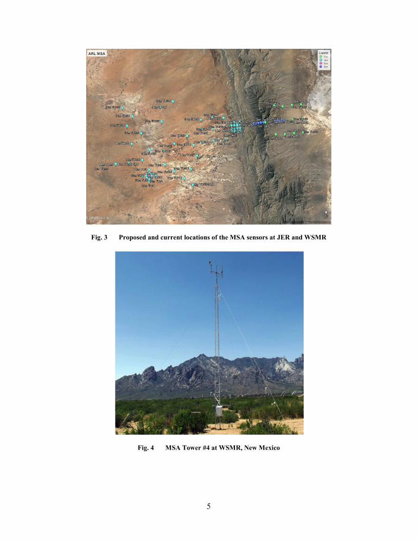
The multiphase program was initiated with a “proof of concept”, which included five equally spaced meteorological towers at WSMR. Today there are 62 towers over the complex terrain of WSMR and in the flatter terrain of the JER. Figure 3 shows the locations of the towers, although these towers can be moved or adjusted based on the mission involved. The blue marks in Fig. 3 show the current location of the towers, while the purple and green marks show where future towers will be built.
The MSA tower design (Fig. 4) included a portable, lightweight aluminum tower with sensors mounted on the 2- and 10-m levels. The data acquisition systems (DAS) were divided into two categories: thermodynamic and dynamic DAS. A Campbell Scientific (Logan, Utah) CR23X Micrologger assimilated the thermodynamic 1-min averaged data. The variables consisted of pressure, temperature (2- and 10-m above ground level [AGL]), relative humidity (2-m AGL), and insolation (2-m AGL). As seen in Fig. 5, the dynamic data originated from two RM Young (Traverse City, Michigan) 81000 Ultrasonic anemometers (2- and 10-m AGL) sampling at 20 Hz. The variables acquired were wind speed, wind direction, u-component, v-component, w-component, speed of sound, and sonic temperature. The raw dynamic data were preserved in files on a laptop computer, then reduced to 1-min averages. The dynamic and thermodynamic 1-min averages were merged with the thermodynamic data. A Digi International (Hopkins, Minnesota) Edgeport RS-232 multiport adapter bridged the two data resources. A system clock on each tower was synchronized using the Network Time Protocol.
5
Fig. 3 Proposed and current locations of the MSA sensors at JER and WSMR
Fig. 4 MSA Tower #4 at WSMR, New Mexico

6
Fig. 5 10-m tower (Climatronics Corp 2014). Used with permission from David W Gilmore, Met One Instruments, Inc., Climatronics Division.
Electrical power for the remotely located towers came from a photovoltaic panel, charge controller, and battery storage unit, specifically tailored to support the temporary Phase I tower configuration. The direct current electronics received a direct feed from the battery, whereas, the alternating current requirements of the computer and wireless adapters (communications) used an inverter.
The initial data flow required a daily download of data from each tower, manual maintenance and monitoring of each tower, and a constant time synchronization check. Once the wireless technology could be installed, these three functions were done through a remote access.
Data processing began with the averaging and merging of thermodynamic and dynamic data. Plots of the time series of each sensor were created and reviewed daily.
7
4. Fundamentals of Flow in Complex Terrain
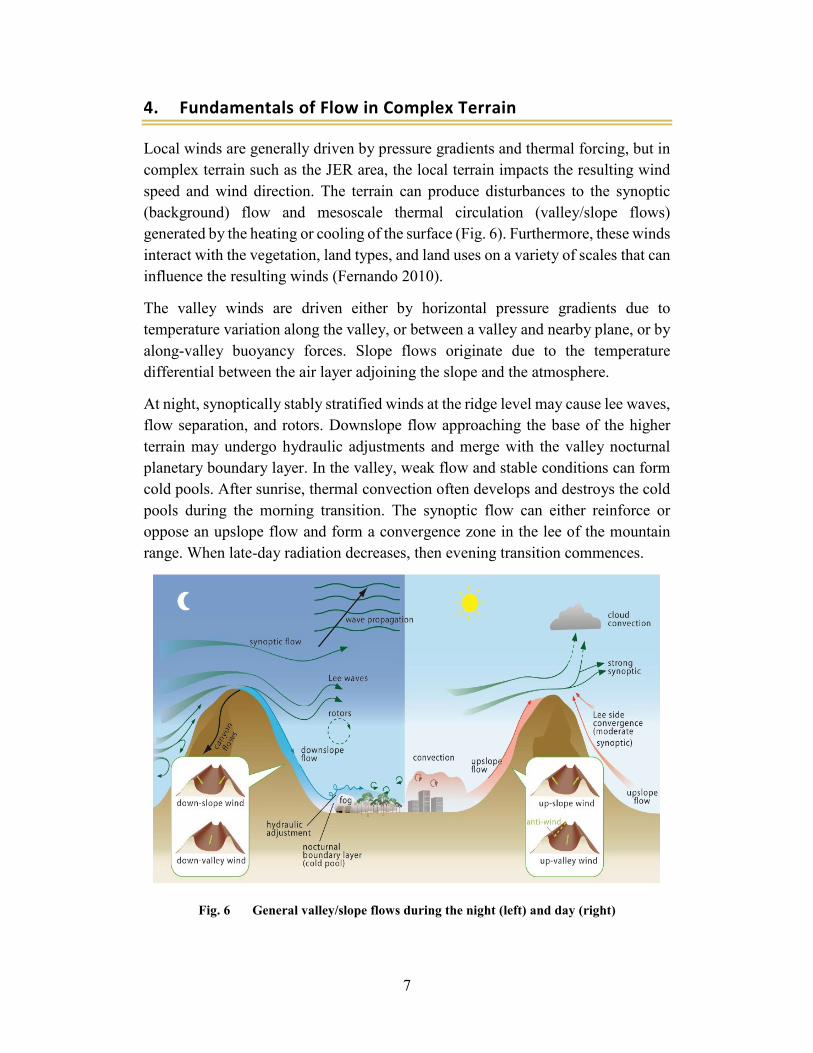
Local winds are generally driven by pressure gradients and thermal forcing, but in complex terrain such as the JER area, the local terrain impacts the resulting wind speed and wind direction. The terrain can produce disturbances to the synoptic (background) flow and mesoscale thermal circulation (valley/slope flows) generated by the heating or cooling of the surface (Fig. 6). Furthermore, these winds interact with the vegetation, land types, and land uses on a variety of scales that can influence the resulting winds (Fernando 2010).
The valley winds are driven either by horizontal pressure gradients due to temperature variation along the valley, or between a valley and nearby plane, or by along-valley buoyancy forces. Slope flows originate due to the temperature differential between the air layer adjoining the slope and the atmosphere.
At night, synoptically stably stratified winds at the ridge level may cause lee waves, flow separation, and rotors. Downslope flow approaching the base of the higher terrain may undergo hydraulic adjustments and merge with the valley nocturnal planetary boundary layer. In the valley, weak flow and stable conditions can form cold pools. After sunrise, thermal convection often develops and destroys the cold pools during the morning transition. The synoptic flow can either reinforce or oppose an upslope flow and form a convergence zone in the lee of the mountain range. When late-day radiation decreases, then evening transition commences.
Fig. 6 General valley/slope flows during the night (left) and day (right)
8
The thermal circulation is dominant in areas of weak synoptic forcing (Whiteman 2000). Downslope winds are stably stratified and are devoid of significant turbulence levels, effective turbulence and heat/mass transport mechanism, and mixing is weak. Meanwhile, during upslope flow the turbulence is intense, vertical transport is strong, and a thick flow layer is formed. However, in cases of stronger synoptic flow surface, winds can increase when air flows over a high mountain ridge with a steep lee slope. These winds most often occur at many locations in the middle latitudes. The downslope winds refer to winds generated as a deeper layer of air is forced over topography. Typically, the downslope wind event is accompanied by an increase in the surface temperature and a drop in surface dew point. The dynamics governing the development of strong downslope winds are analogous to those governing the rapid increase in speed when water goes from a slow velocity upstream to a layer of high-velocity fluid on the downstream face. In such cases, a turbulent hydraulic jump develops downstream where high-speed flow decelerates back to the ambient velocity of the fluid.
During fair-weather conditions, mountain slopes often exhibit upslope flows of air during the day (Atkinson 1981). During the day, an air parcel right above the slope’s surface has a higher potential temperature and therefore, lower density than an air parcel at the same height further away from the heated surface. The result is a combination of two forces acting upon the air parcel above the mountain slope: a pressure gradient force pushing the column of air toward the slope, and a buoyancy force driving the air parcel upward. The sum of both forces results in air being moved parallel to the slope and replaced by air coming from the plain.
An explanation of the upslope–downslope flow transition is given by Villagrasa et al. (2013) where they point out that the transition is driven by the change in sign of the sensible heat flux on the sidewalls/slopes as they become shaded from direct solar radiation. Typically, this precedes the up-valley–down-valley transition. Beginning with an existing upslope flow, Hunt et al. (2003) developed a simplified theoretical model to describe the upslope-to-downslope transition over a gentle slope. The transition occurs via the formulation of a stagnant frontal region at a certain distance upslope. This distance depends on the initial buoyancy, the cooling time scale, and former upslope velocity. The transition front may move up or down the slope based the direction of the shadow. Fernando et al. (2013) showed multiple fronts from different slopes during the evening transition before the downslope ensued. The flow transition for slopes on the valley sidewalls is embedded in the larger-scale along-valley circulations. During the day, the upslope wind is modulated by its interaction with the convective boundary layer evolution within the valley atmosphere (Seradin and Zardi 2010). At night, the downslope current is affected either by the growth of a cold pool at the base of the slope (Cuxart et al.

9
2007) or interaction with the down-valley current. Onset of drainage is produced after the reversal of sensible heat flux.
Work done by Wang et al. (1995) noted on occasion, in certain environments, a nocturnal low-level jet (LLJ) developed. In this case, the higher terrain was to the west and a southerly LLJ developed. After sunset there is a wind peak with a maximum at least 2 m/s greater than the wind before sunset. Duration was no more than one or two hours. The layer of the peak speed was shallow and wind speeds very low above the layer.
5. Examples of Wind Flow at JER
From November 2014 to February 2017, 32 model runs centered on the headquarters of JER were completed. A variety of weather types and conditions were tested to study the wind flows at JER. This included 14 days listed as “windy” days with traditional spring winds over JER and the area. Eleven days were quiescent days with generally fair skies and light winds. Five days featured thunderstorms, severe weather, and well-developed gust fronts. Two days were run during the southwest summer monsoon. Three cases were run with four-dimensional data assimilation (FDDA) and non-FDDA included. These days were all selected because they presented the WRF with certain “challenges” that were desirable to study over the local area.
5.1 12 Jan 2016: Light Wind Case
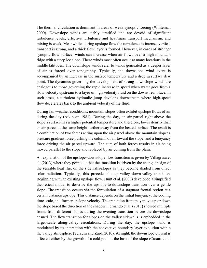
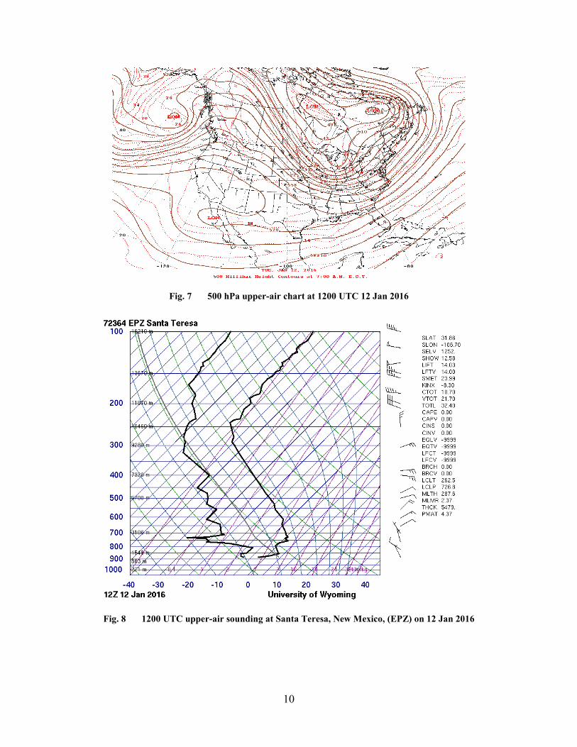
The 500-hPa upper-air map at 1200 UTC (Fig. 7) shows a deep trough of lower heights over the upper Midwest with a strong upper air high over the southwest United States with only a weak undercutting upper low in northern Mexico. New Mexico and the JER area are under subsiding air with light winds. The upper-air observation at 1200 UTC (Fig. 8) at nearby Santa Teresa, New Mexico, (EPZ) shows a dry profile with light winds variable in direction, below 400 hPa. There is a strong but shallow inversion noted near the surface with another inversion layer between 780 and 750 hPa. In Fig. 9, the surface map shows high pressure with precipitation-free weather over the western United States, including New Mexico.
10
Fig. 7 500 hPa upper-air chart at 1200 UTC 12 Jan 2016
Fig. 8 1200 UTC upper-air sounding at Santa Teresa, New Mexico, (EPZ) on 12 Jan 2016

11
Fig. 9 Surface weather chart at 1200 UTC (0600 local daylight time [LDT]) 12 Jan 2016
The model run began at 1200 UTC for a 24-h duration over the JER area, which included much of WSMR. Pressure gradients were light, which meant the flow was dependent on the temperature field and topographic effects. The JER headquarters are located at the center of the grid in Fig. 10. At 1300 UTC, the forecasted wind speeds were under 4 m/s over much of JER. There are slightly higher winds to the south while the strongest winds are over the higher peaks of Picacho and the Dona Ana mountains. There are light, down-valley winds noted over much of the grid. During the night, cold air flows down the slope and collects in the valley, which results in a pressure increase in the valley causing a cold pool with light winds on the valley floor. This agrees with the work of McNider and Pielke (1984).

12
Fig. 10 Surface winds and speeds (m/s) on at 1300 UTC 12 Jan 2016
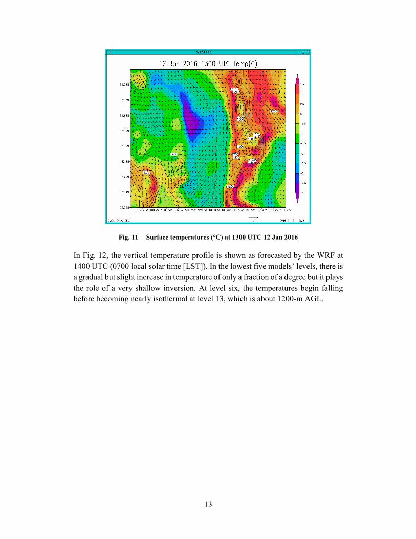
In Fig. 11, the temperatures in degrees Celsius are displayed on the surface at 1300 UTC along with the wind barbs. There is a distinct cold pool in the central valley of JER with lowest temperatures around –4 °C. Meanwhile, in areas of downslope winds there are higher temperatures (1.5 °C) along both the east and west slopes of the north–south San Andres Mountains. Given the predominant down-valley flow, the winds over the higher terrain run from the north to south over the Dona Ana Mountains with resulting higher temperatures. An interesting feature in Fig. 11 is seen on the east side of the cold pool on the foothills or lower slope of the mountain range. To the south of the cold pool, winds are light (1 to 2 m/s) from a general southerly direction. This follows the trend of the down-valley wind, perhaps influenced by the drainage winds off the terrain. Meanwhile, north and east of the cold pool the winds at the base of the mountain wall are from the south. Perhaps the cold pool, located in a localized valley, acts to deflect the wind, or it could be influenced by the vegetation differences in the immediate area.
13
Fig. 11 Surface temperatures (°C) at 1300 UTC 12 Jan 2016
In Fig. 12, the vertical temperature profile is shown as forecasted by the WRF at 1400 UTC (0700 local solar time [LST]). In the lowest five models’ levels, there is a gradual but slight increase in temperature of only a fraction of a degree but it plays the role of a very shallow inversion. At level six, the temperatures begin falling before becoming nearly isothermal at level 13, which is about 1200-m AGL.

14
Fig. 12 Vertical temperature profile (°C) over JER headquarters at 1400 UTC 12 Jan 2016
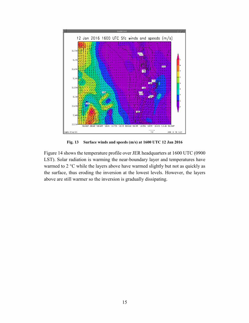
By 1600 UTC (0900 LST), as seen in Fig. 13, the winds are gradually shifting to an upslope direction, especially on the east slope of the San Andres Mountains. The winds are light and variable on the west side of the mountain range.
15
Fig. 13 Surface winds and speeds (m/s) at 1600 UTC 12 Jan 2016
Figure 14 shows the temperature profile over JER headquarters at 1600 UTC (0900 LST). Solar radiation is warming the near-boundary layer and temperatures have warmed to 2 °C while the layers above have warmed slightly but not as quickly as the surface, thus eroding the inversion at the lowest levels. However, the layers above are still warmer so the inversion is gradually dissipating.

16
Fig. 14 Vertical temperature profile (°C) over JER headquarters at 1600 UTC 12 Jan 2016
By afternoon, at 2100 UTC (1400 LST), as shown in Fig. 15, winds over the southern part of JER are light and variable, while there still is a down-valley wind to the west along with weak upslope winds on both the east and west sides of the San Andres Mountain range. An interesting feature is seen on the northern area of the plot (32.75° N and –106.75° W) where an area of light winds (1 to 1.5 m/s) are surrounded by stronger winds from different directions, with south winds (up valley) to the east side and north winds (down valley) on the west side of the area.

17
Fig. 15 Surface winds and speeds (m/s) at 2100 UTC 12 Jan 2016
Meanwhile, the vertical profile is shown at 2100 UTC (1400 LST) over JER headquarters in Fig. 16. The surface has warmed to 5.5 °C and the layers above have not warmed as quickly, thus totally eroding the morning inversion, as would be expected.

18
Fig. 16 Vertical temperature profile (°C) over JER headquarters at 2100 UTC 12 Jan 2016
Figure 17 displays the temperature field and wind plot over the JER area at 2200 UTC (1500 LST). Again, there is an apparent “eddy” in the flow where the warmest temperatures are near 32.70 °N and 106.7 °W. There is a general phasing of the upslope flow and the up-valley flow on the east side of JER as it slopes toward the mountains. Surprisingly, the flow is still from north to south on the west side of the plot, still a down-valley wind.
19
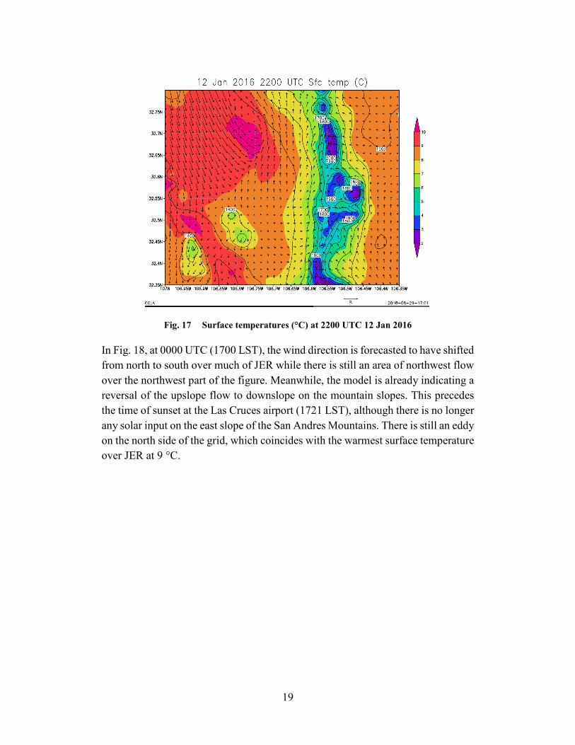
Fig. 17 Surface temperatures (°C) at 2200 UTC 12 Jan 2016
In Fig. 18, at 0000 UTC (1700 LST), the wind direction is forecasted to have shifted from north to south over much of JER while there is still an area of northwest flow over the northwest part of the figure. Meanwhile, the model is already indicating a reversal of the upslope flow to downslope on the mountain slopes. This precedes the time of sunset at the Las Cruces airport (1721 LST), although there is no longer any solar input on the east slope of the San Andres Mountains. There is still an eddy on the north side of the grid, which coincides with the warmest surface temperature over JER at 9 °C.
20
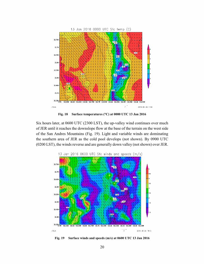
Fig. 18 Surface temperatures (°C) at 0000 UTC 13 Jan 2016
Six hours later, at 0600 UTC (2300 LST), the up-valley wind continues over much of JER until it reaches the downslope flow at the base of the terrain on the west side of the San Andres Mountains (Fig. 19). Light and variable winds are dominating the southern area of JER as the cold pool develops (not shown). By 0900 UTC (0200 LST), the winds reverse and are generally down valley (not shown) over JER.
Fig. 19 Surface winds and speeds (m/s) at 0600 UTC 13 Jan 2016
21
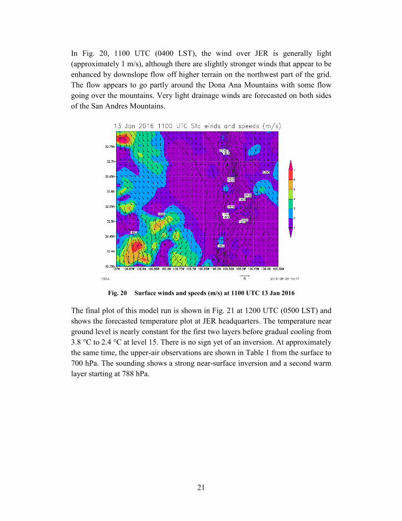
In Fig. 20, 1100 UTC (0400 LST), the wind over JER is generally light (approximately 1 m/s), although there are slightly stronger winds that appear to be enhanced by downslope flow off higher terrain on the northwest part of the grid. The flow appears to go partly around the Dona Ana Mountains with some flow going over the mountains. Very light drainage winds are forecasted on both sides of the San Andres Mountains.
Fig. 20 Surface winds and speeds (m/s) at 1100 UTC 13 Jan 2016
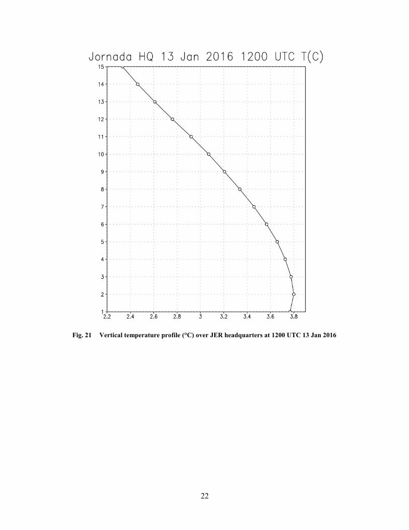
The final plot of this model run is shown in Fig. 21 at 1200 UTC (0500 LST) and shows the forecasted temperature plot at JER headquarters. The temperature near ground level is nearly constant for the first two layers before gradual cooling from 3.8 °C to 2.4 °C at level 15. There is no sign yet of an inversion. At approximately the same time, the upper-air observations are shown in Table 1 from the surface to 700 hPa. The sounding shows a strong near-surface inversion and a second warm layer starting at 788 hPa.
22
Fig. 21 Vertical temperature profile (°C) over JER headquarters at 1200 UTC 13 Jan 2016

23
Table 1 Sounding at 1200 UTC 13 Jan 2016 from surface to 700 hPa at Santa Teresa, New Mexico (EPZ)
PRES (hPA)
HGHT (m)
TEMP (°C)
DWPT (°C)
RELH (%)
MIXR (g/kg)
DRCT (deg)
SKNT (knot)
THTA (K)
THTE (K)
THTV (K)
1000.0 196 … … … … … … … … …
925.0 841 … … … … … … … … …
879.0 1252 –2.1 –6.3 73 2.73 25 4 281.2 289.1 281.7
876.0 1280 1.2 –7.8 51 2.44 20 4 284.9 292.2 285.4
871.0 1327 3.2 –6.8 48 2.65 13 4 287.5 295.4 287.9
864.0 1394 4.2 –4.8 52 3.11 2 5 289.2 298.4 289.7
850.0 1530 4.2 –5.8 48 2.93 340 5 290.5 299.3 291.1
841.0 1616 3.6 –5.4 52 3.05 334 5 290.8 300.0 291.3
821.0 1812 3.0 –11.0 35 2.02 321 5 292.2 298.4 292.5
819.2 1829 2.9 –11.2 35 2.00 320 5 292.2 298.4 292.6
800.0 2021 2.0 –13.0 32 1.77 232 4 293.3 298.8 293.6
788.9 2134 3.9 –21.4 14 0.89 180 3 296.4 299.4 296.6
787.0 2153 4.2 –22.8 12 0.78 181 3 297.0 299.6 297.1
772.0 2310 4.4 –24.6 10 0.68 189 4 298.9 301.1 299.0
759.9 2438 4.0 –23.9 11 0.73 195 5 299.7 302.2 299.9
731.8 2743 2.9 –22.3 14 0.88 20 3 301.8 304.7 301.9
730.0 2763 2.8 –22.2 14 0.89 18 3 301.9 304.9 302.1
700.0 3101 0.6 –33.4 6 0.33 345 7 303.1 304.3 303.2
5.2 10 Apr 2019: Strong Wind Case
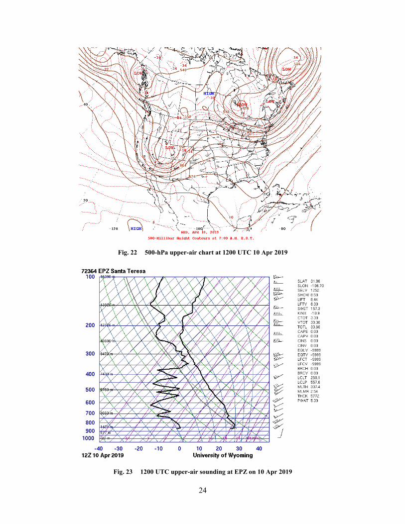
The 1200 UTC upper-air map on 10 April 2019 indicated a deep, upper low over central Utah with a 5520-m center and a 500-hPa cold core of –26 °C over the Nevada/Utah border (Fig. 22). This upper low was being kicked out of a shortwave over British Columbia. There was a ridge of high heights over the central United States that enhanced the southwesterly flow over New Mexico. The 1200 UTC upper-air sounding at EPZ, as displayed in Fig. 23, shows this deep southwesterly to westerly flow with 53 kts of wind at 700 hPA, 56 kts at 500 hPa, and 82 kts at 250 hPa. The sounding is very typical for windy spring days in the southwest United States.
24
Fig. 22 500-hPa upper-air chart at 1200 UTC 10 Apr 2019
Fig. 23 1200 UTC upper-air sounding at EPZ on 10 Apr 2019

25
The main features on the surface weather map (Fig. 24) at 1200 UTC 10 April 2019 shows a deep low pressure over Colorado to a secondary low over northwest New Mexico with a cold front across western New Mexico.
Fig. 24 Surface weather chart at 1200 UTC (0600 LDT) 10 Apr 2019
At 1200 UTC, as seen in Fig. 25, the prevailing forecasted wind direction is from the southwest across most of the domain, but winds are from the south over the JER in response to the pressure gradient force due to the lower pressure over Colorado. The strongest predicted winds are over the highest terrain with wind speeds of 19 m/s on the downslope side of the mountains to the east. The temperature forecast is typical of a strong wind event over the region with the warmest temperatures on the downslope side of the mountains and the coldest temperatures over the mountain peaks. There is no evidence of a cold pool in the usual area of the JER due to the strong winds and mixing.

26
Fig. 25 Forecasted surface temperature and wind direction at 1200 UTC 10 Apr 2019
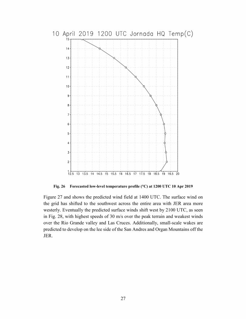
The forecasted upper-air temperature profile in Fig. 26 shows a slight inversion near the surface, then an isothermal layer to model level 7 before cooling significantly to model level 15 (4500 AGL). This agrees favorably with the observed upper-air temperature field as seen in Fig. 23.
27
Fig. 26 Forecasted low-level temperature profile (°C) at 1200 UTC 10 Apr 2019
Figure 27 and shows the predicted wind field at 1400 UTC. The surface wind on the grid has shifted to the southwest across the entire area with JER area more westerly. Eventually the predicted surface winds shift west by 2100 UTC, as seen in Fig. 28, with highest speeds of 30 m/s over the peak terrain and weakest winds over the Rio Grande valley and Las Cruces. Additionally, small-scale wakes are predicted to develop on the lee side of the San Andres and Organ Mountains off the JER.

28
Fig. 27 Forecasted wind speed (m/s) and direction at 1400 UTC 10 Apr 2019
Fig. 28 Forecasted wind speed (m/s) and direction at 2100 UTC 10 Apr 2019
In Fig. 29, at 1200 UTC 11 April 2019, the winds over JER are forecasted to be from the south and have decreased to under 4 m/s. The general trend of a windy day sequence is a quick turn to southwest winds and a gradual increase of afternoon wind speeds with peak winds generally in the middle-to-late afternoon. The wind direction remains from the southwest or west through the evening hours, but toward sunrise the wind direction will switch to the south or north based on the resulting pressure gradient.

29
Fig. 29 Forecasted wind speed (m/s) and direction at 1200 UTC 11 Apr 2019
6. Discussion
While the previous cases are “traditional” cases for light wind days and stronger wind days, there are very complicated processes going on at many different temporal and spatial scales. These interactions make for intriguing studies over the JER and provide much motivation for using the MSA to validate and improve the model as well as gain a better understanding of all these interactions.
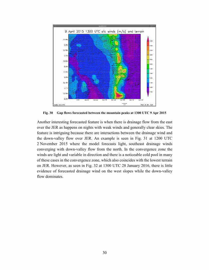
The WRF does capture many of these complex flows as already seen in this report. In Fig. 30, at 1300 UTC 9 April 2015 the forecast is for light down-valley morning flow as well as downslope flow coming off the higher terrain. However, the model shows gap flow in the lower elevations of the mountains.
30
Fig. 30 Gap flows forecasted between the mountain peaks at 1300 UTC 9 Apr 2015
Another interesting forecasted feature is when there is drainage flow from the east over the JER as happens on nights with weak winds and generally clear skies. The feature is intriguing because there are interactions between the drainage wind and the down-valley flow over JER. An example is seen in Fig. 31 at 1200 UTC 2 November 2015 where the model forecasts light, southeast drainage winds converging with down-valley flow from the north. In the convergence zone the winds are light and variable in direction and there is a noticeable cold pool in many of these cases in the convergence zone, which also coincides with the lowest terrain on JER. However, as seen in Fig. 32 at 1300 UTC 28 January 2016, there is little evidence of forecasted drainage wind on the west slopes while the down-valley flow dominates.

31
Fig. 31 Forecasted transitional flow over JER at 1200 UTC 2 Nov 2015
Fig. 32 Weak drainage flow predicted on the west slope converges with down-valley flow over JER at 1300 UTC 28 Jan 2016
Another feature of the region is the variable morning temperature pattern that is highly based on the terrain and the wind flow at night during quiescent weather patterns. An example is shown in Fig. 33 where forecasted temperature ranges at 1300 UTC 13 October 2015 range from 20 ℃ on the downslope western slopes to as cold as 11 ℃ in the valley locations of JER (Fig. 34). Verification at that time

32
using https://mesowest.utah.edu indicates agreement on most of the trends with JER headquarters reporting a temperature of 10 ℃ and Organ, New Mexico, at 19 ℃. The model wind field also shows accuracy with northeast drainage wind to the southwest of JER and slight southeast drainage winds over Organ, New Mexico.
Fig. 33 Forecasted temperatures (℃) for southern New Mexico at 1300 UTC 13 Oct 2015
Fig. 34 Verified temperatures from 1300 UTC 13 Oct 2015 over southern New Mexico using https://mesowest.utah.edu
33
Further studies can also focus on the up-valley and down-valley flows, especially the timing involved. As shown earlier for the 12 January 2016 case, the morning down-valley flow is forecasted to persist through much of the day as displayed in the sequence of Fig. 10 (1300 UTC), Fig. 15 (2100 UTC), and Fig. 18 (0000 UTC) on 13 January 2016 where the up-valley flow finally is forecasted to occur. The same thing occurs at night as seen in the sequence in Fig. 19 (0600 UTC) and Fig. 21 (1100) when eventually a down-valley flow becomes pronounced. In other studies, such as Stewart et al. (2002) in Utah, the morning transition can start as early as 0600 local or as late as 1100 local time and the evening transition has been found to occur quicker than the morning transition at Salt Lake City, Utah. In a study in Idaho, it was found the upslope/downslope transition takes 1–2 h, but the up-valley and down-valley transition may take 5–6 h to commence.
Perhaps one of the more complex wind structure issues are the winds near the Dona Ana Mountains to the west of JER and the influence of the mountains over the JER.
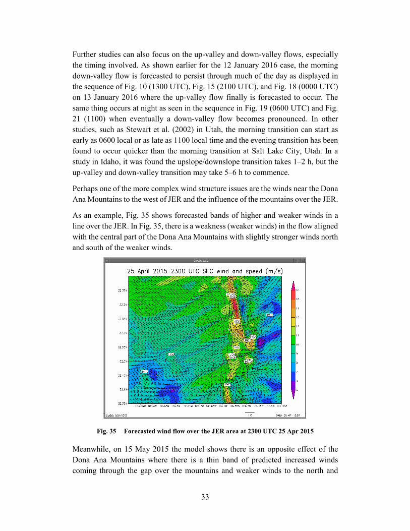
As an example, Fig. 35 shows forecasted bands of higher and weaker winds in a line over the JER. In Fig. 35, there is a weakness (weaker winds) in the flow aligned with the central part of the Dona Ana Mountains with slightly stronger winds north and south of the weaker winds.
Fig. 35 Forecasted wind flow over the JER area at 2300 UTC 25 Apr 2015
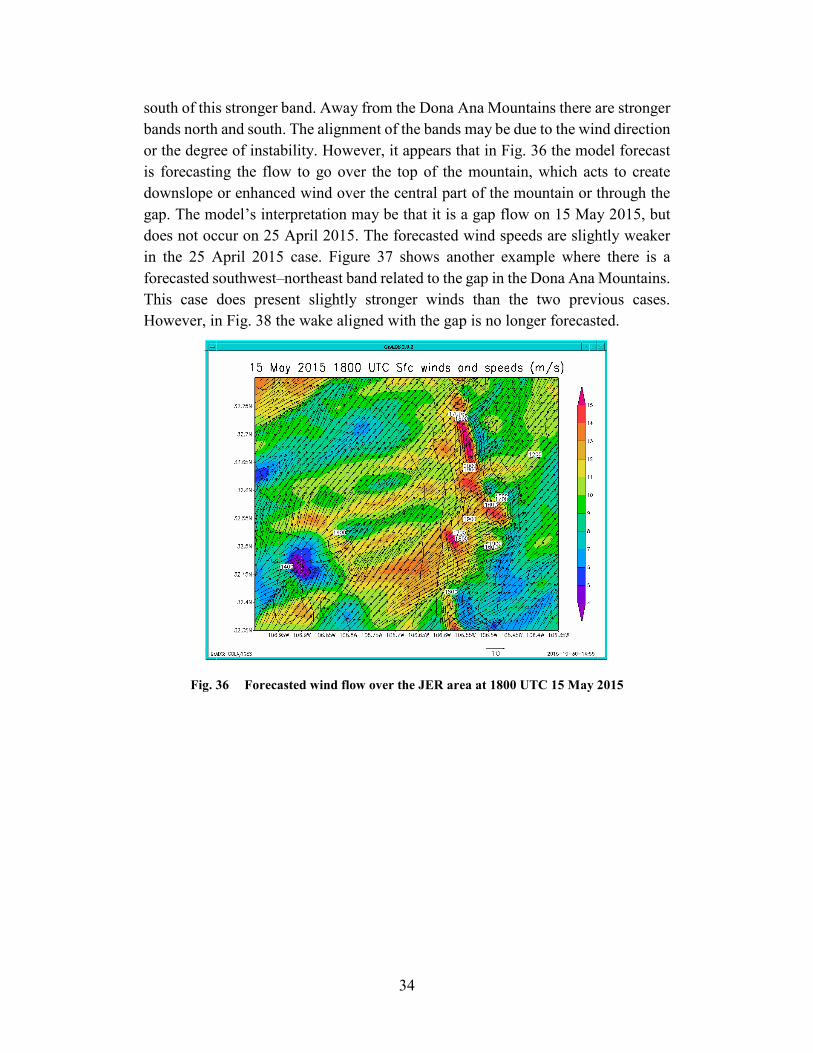
Meanwhile, on 15 May 2015 the model shows there is an opposite effect of the Dona Ana Mountains where there is a thin band of predicted increased winds coming through the gap over the mountains and weaker winds to the north and
34
south of this stronger band. Away from the Dona Ana Mountains there are stronger bands north and south. The alignment of the bands may be due to the wind direction or the degree of instability. However, it appears that in Fig. 36 the model forecast is forecasting the flow to go over the top of the mountain, which acts to create downslope or enhanced wind over the central part of the mountain or through the gap. The model’s interpretation may be that it is a gap flow on 15 May 2015, but does not occur on 25 April 2015. The forecasted wind speeds are slightly weaker in the 25 April 2015 case. Figure 37 shows another example where there is a forecasted southwest–northeast band related to the gap in the Dona Ana Mountains. This case does present slightly stronger winds than the two previous cases. However, in Fig. 38 the wake aligned with the gap is no longer forecasted.
Fig. 36 Forecasted wind flow over the JER area at 1800 UTC 15 May 2015

35
Fig. 37 Flow over the JER area at 2300 UTC 12 Apr 2018
Fig. 38 Forecasted flow over the JER at 0000 UTC 13 Apr 2018
In all three of these cases the predicted wind direction is nearly identical, although there are only marginal differences in the wind speed. According to Whiteman (2000), the factors that affect terrain-forced flows are the stability of the air

36
approaching the mountain, the speed of the air flow, and topographic characteristics of the terrain. Unstable air can more easily be carried over a mountain barrier while stable air is more resistant to being lifted so it might flow around the barrier, go through gaps, or be blocked. Additionally, the height and length of the mountain barrier helps determine whether the air goes over or around the barrier while the shape of the mountains affects the wind flow also. It then becomes a question as to what wind speed and stability are needed or responsible for different actions of the wind with respect to the terrain.
7. Conclusion
ARL has responded to an observation weakness by building an observational data resource specifically designed to address the “Army-scale”, high-resolution atmospheric model validation and verification issues. This new effort is called the MSA. The role of the MSA is to improve high-resolution atmospheric models for Army decision making. The MSA will provide continual data, which allows scientists to compare output of the WRF-ARW with real-time observations. Modeling efforts have centered on running the WRF over the JER in an attempt to discover significant trends in the model and determine areas to study using the real-time MSA data. Currently, most of the study is focused on surface observation and model output in the boundary layer. Based on these model runs on both tranquil and windy days, many questions are raised using the model output. The models have numerous interactions between synoptic, mesoscale, and microscale flows and in this complex terrain it becomes an intricate problem of the interaction of the slope and valley flow that can create areas of convergence and divergence over the grid, which in turn can impact the local sensible weather. Using a large number of model runs, the wind and temperature fields were studied in anticipation of comparing these model runs to real-time MSA data. Among the topics studied are the interaction of slope and valley winds, the onset of the up-valley and down-valley flows, and the influence of the local terrain on wind flows. Currently, sub-kilometer models of JER are being run so subject matter such as boundary fluxes, wind channeling, and soil and land use will be better understood. Supplementary studies of dust raised, fires, and the summer monsoonal patterns will afford a better understanding of the processes affecting the local area as well as areas of concern to the Army.

37
8. References
Atkinson BW. Mesoscale atmospheric circulations. London (England): Academic Press; 1981.
Cuxart J, Jiménez MA, Martinez D. Nocturnal meso-beta and katabatic flows on a midlatitude island. Mon Weather Rev. 2007;135(3):918–932.
Deng A, Stauffer D, Gaudet B, Dudhia J, Hacker J, Bruyere C, Wu W, Vandenberghe F, Liu Y, Bourgeois A. Update on WRF-ARW end-to-end multi-scale FDDA system. In: 10th Annual WRF Users' Workshop, NCAR, 1.9; 2009 June 23–26; Boulder, CO [accessed 2019 Sep 5]. http://www.mmm.ucar.edu/wrf/users/workshops/WS2009/abstracts/1-09.pdf.
Fernando HJS. Fluid dynamics of urban atmospheres in complex terrain. Annu Rev Fluid Mech. 2010;42:365–389.
Fernando HJS, Verhoef B, Di Sabatino S, Leo LS, Park S. The phoenix evening transition flow experiment (TRANSFLEX). Bound-Lay Meteorol. 2013;147(3):443–468.
Havstad KM, Kustas WP, Rango A, Ritchie JC, Schmugge TJ. Jornada experimental range: a unique arid land location for experiments to validate satellite systems. Remote Sens Environ. 2000;74(1):13–25.
Hunt JCR, Fernando HJS, Princevac M. Unsteady thermally driven flows on gentle slopes. J Atmos Sci. 2003;60:2169–2182.
Janjić Z. Nonsingular implantation of the Mellor-Yamada level 2.5 scheme in the NCEP meso model. College Park (MD): National Centers for Environmental Prediction; 2001. Report No.: 437. http://www.lib.ncep.noaa.gov/ ncepofficenotes/files/on437.pdf.
Lee JA, Kolczynski WC, McCandless T, Haupt SE. An objective methodology for configuring and down-selecting an NWP ensemble for low-level wind prediction. Mon Weather Rev. 2012;140(7):2270–2286.
McNider RT, Pielke RA. Numerical simulation of slope and mountain flows. J Clim Appl Meteorol. 1984;23(10):1441–1453.
Passner JE. Low-level turbulence from fine-scale models. White Sands Missile Range (NM): Army Research Laboratory (US); 2014. Report No.: ARL-TR-6847.
38
Seradin S, Zardi D. Structure of the atmospheric boundary layer in the vicinity of a developing upslope flow system: a numerical model study. J Atmos Sci. 2010;67:1171–1185.
Skamarock WC, Klemp JB, Dudhia J, Gill DO, Barker DM, Duda MG, Huang X-Y, Wang W, Powers JG. A description of the advanced research WRF version 3. Boulder (CO); National Center for Atmospheric Research; 2008. NCAR Technical Note. Report No.: 475 [accessed 2019 August 2]. http://www2.mmm.ucar.edu/wrf/users/ docs/ arw_v3.pdf.
Stewart JQ, Whiteman CD, Steenburgh WJ, Bian X. A climatological study of thermally driven wind systems of the U.S. Intermountain West. B Am Meteorol Soc. 2002;83:699–708.
Whiteman CD. Mountain meteorology: fundamentals and applications. New York (NY): Oxford University Press; 2000.
Vaucher G, Swanson J, Raby J, Foley T, Harrison S, Brice R, D’Arcy S, Creegan E. Meteorological sensor array (MSA)—phase 1, volume 1 (“proof of concept” overview). White Sands Missile Range (NM): Army Research Laboratory (US); 2014. Report No.: ARL-TR-7058.
Villagrasa DM, Lehner M, Whiteman CD, Hoch SW, Cuxart J. The upslope-downslope flow transition on a basin sidewall. J Appl Meteorol Clim. 2013;52:2715–2734.
Wang Q, Zhu P, Wang B, Jiang R. Analysis of nighttime drainage wind in the HEIFE region. J Meteorol Soc Japan. 1995;73(6):1285–1291.

39
List of Symbols, Abbreviations, and Acronyms
ABL atmospheric boundary layer
AGL above ground level
ARL US Army Research Laboratory
DAS data acquisition systems
EPZ Santa Teresa, NM
FDDA four-dimensional data assimilation
GFS Global Forecast System
hPa hectopascal
JER Jornada Experimental Range
LDT local daylight time
LLJ low-level jet
LST local solar time
MSA Meteorological Sensor Array
MYJ Mellor-Yamada-Janjić
NAM North American Mesoscale Model
TKE turbulent kinetic energy
UTC Coordinated Universal Time
WRF Weather Research and Forecasting
WRF-ARW Advanced Research version of the Weather Research and Forecasting model
WSMR White Sands Missile Range

40
1 DEFENSE TECHNICAL (PDF) INFORMATION CTR DTIC OCA 1 CCDC ARL (PDF) FCDD RLD CL TECH LIB 1 GOVT PRINTG OFC (PDF) A MALHOTRA 1 CCDC ARL (PDF) FCDD RLC EM J PASSNER