advanced quantum information theorycsxam/teaching/aqit2016/lecture... · the eld of quantum...
TRANSCRIPT

CDT in Quantum Engineering Spring 2016
ADVANCED QUANTUM INFORMATION THEORY
Lecture notes
Ashley Montanaro, University of [email protected]
Contents
1 Introduction 2
2 Classical and quantum computational complexity 4
3 Grover’s algorithm 10
4 The Quantum Fourier Transform and periodicity 17
5 Integer factorisation 22
6 Phase estimation 28
7 Hamiltonian simulation 31
8 Quantum walk 35
9 Noise and the framework of quantum channels 45
10 Quantum error-correction 50
11 Quantum state discrimination and tomography 57
Health warning: There are likely to be changes and corrections to these notes throughout the unit.For updates, see http://www.maths.bris.ac.uk/~csxam/aqit2016/.
Version 1.5 (February 26, 2016).
1
1 Introduction
The field of quantum information theory studies the remarkable ways in which quantum information– and the processing thereof – differs from information stored in classical systems. Nowhere isthis difference more pronounced than the dramatic speedups obtained by quantum computationover classical computation. These notes aim to cover (some of) the theoretical topics which anyself-respecting quantum information theorist, or experimentalist working in the field of quantuminformation processing, should know. These include the famous algorithms of Shor and Grover, andthe simulation of quantum systems; the more recent topic of quantum walk algorithms; decoherenceand quantum error-correction.
1.1 Complementary reading
These lecture notes have benefited significantly from the expositions in the following lecture courses,which may be of interest for background reading:
• Quantum Computation, Richard Jozsa, University of Cambridgehttp://www.qi.damtp.cam.ac.uk/node/261
The material here on the QFT and Shor’s algorithm follows this exposition closely.
• Quantum Algorithms, Andrew Childs, University of Marylandhttp://cs.umd.edu/~amchilds/qa/
A combination of lecture notes for three graduate courses. The material here on quantumwalk algorithms is based on the exposition in these notes.
• Theory of Quantum Information, John Watrous, University of Waterloohttps://cs.uwaterloo.ca/~watrous/LectureNotes.html
A particularly useful resource for the theory of quantum channels.
The following books and survey papers may also be useful:
• Quantum Computation and Quantum Information, Nielsen and ChuangCambridge University Press, 2001The Bible of quantum computing.
• Classical and Quantum Computation, Kitaev, Shen and VyalyiAmerican Mathematical Society, 2002A more concise introduction to many important topics in quantum computation.
• Quantum algorithms for algebraic problems, Childs and van DamReviews of Modern Physics, 82:1, 2010; http://arxiv.org/pdf/0812.0380.pdfCovers many other quantum algorithms than those discussed here.
1.2 Notation
We write [n] := 1, . . . , n for the integers between 1 and n. dxe, bxc and bxe denote the smallestinteger y such that y ≥ x, the largest integer z such that z ≤ x, and the closest integer to x,respectively. We use
(nk
)for the binomial coefficient “n choose k”, n!/(k!(n − k)!). Finally, when
we say “bounded-error”, we mean with failure probability upper-bounded by some constant below1/2.
2

We use standard “computer science style” notation relating to asymptotic complexity:
• f(n) = O(g(n)) if there exist real c > 0 and integer n0 ≥ 0 such that for all n ≥ n0,f(n) ≤ c g(n).
• f(n) = Ω(g(n)) if there exist real c > 0 and integer n0 ≥ 0 such that for all n ≥ n0,f(n) ≥ c g(n). Clearly, f(n) = O(g(n)) if and only if g(n) = Ω(f(n)).
• f(n) = Θ(g(n)) if f(n) = O(g(n)) and f(n) = Ω(g(n)).
O, Ω and Θ can be viewed as asymptotic, approximate versions of ≤, ≥ and =.
Box 1: Big-O notation
1.3 Change log
• v1.0: first version covering first part of the 2016 unit.
• v1.1: addition of material on the QFT, periodicity and Shor’s algorithm.
• v1.2: addition of material on phase estimation and Hamiltonian simulation.
• v1.3: addition of material covering the remainder of the unit.
• v1.4: update tomography section to mention recent results.
• v1.5: correct typos in stabilizer quantum error-correction section.
3
2 Classical and quantum computational complexity
Computational complexity theory aims to classify different problems in terms of their difficulty, orin other words the resources required in order to solve them. Two of the most important types ofresources one might study are time (the number of computational steps used by an algorithm solvinga problem) and space (the amount of additional work space used by the algorithm). Classically,the formal model underpinning the notion of an “algorithm” is the Turing machine. We will notgo into details about this here, instead taking the informal approach that the number of steps usedby an algorithm corresponds to the number of lines of code executed when running the algorithm,and the space usage is the amount of memory used by the algorithm. For much more on the topic,see the book Computational Complexity by Papadimitriou, for example.
Rather than looking at the complexity of algorithms for solving one particular instance of aproblem, the theory considers asymptotics: given a family of problems, parametrised by an instancesize (usually denoted n), we study the resources used by the best possible algorithm for solving thatfamily of problems. The term “problem” is used henceforth as shorthand for “family of problems”.A dividing line between efficient and inefficient algorithms is provided by the notion of polynomial-time computation. An algorithm running in time polynomial in n, i.e. O(nc) for some fixed c, isconsidered efficient. For example, consider the following two problems:
• Primality testing: given an integer N expressed as n binary digits, is it a prime number?
• Factorisation: given an integer N expressed as n binary digits, output the prime factors ofN .
As the input is of size n, we would like to solve these problems using an algorithm which runs intime poly(n) (not poly(N)!). No such classical algorithm is known for the factorisation problem;as we will see later, the situation is different for quantum algorithms. However, surprisingly, thereis a polynomial-time classical algorithm for the tantalisingly similar problem of primality testing.
An important class of problems is known as decision problems; these are problems that have ayes-no answer. The first of the above problems is a decision problem, while the second is not. Butit can be made into a decision problem without changing its underlying complexity significantly:
• Factorisation (decision variant): given integers N and K expressed as n binary digits each,does N have a prime factor smaller than K?
It is clear that, if we can solve the usual “search” variant of the factorisation problem, solving thedecision variant is easy. Further, solving the decision variant allows us to solve the search variantof the problem using binary search. Given an integer N whose prime factors we would like todetermine, and an algorithm which solves the decision variant of the factorisation problem, we canuse O(logN) = O(n) evaluations of this algorithm with different values of K to find the smallestprime factor M of N . The other factors can be found by dividing N by M and repeating. This isa simple example of a reduction: conversion of one problem into another.
A natural way to compare the complexity of problems is via the notion of complexity classes,where a complexity class is simply a set of problems. Some important classical complexity classesare:
• P: the class of decision problems which can be solved in polynomial time by a classicalcomputer.
4
• NP: the class of decision problems such that, if the answer is “yes”, there is a proof of thisfact which can be verified in polynomial time by a classical computer.
• PSPACE: the class of decision problems which can be solved in polynomial space by a classicalcomputer.
Primality testing is in P, although this was shown for the first time only in 2002. The decisionvariant of factorisation is in NP, because given a claimed prime factor of N smaller than K, it canbe easily checked whether the claim is correct. However, factorisation is not known to be in P. Everyproblem in P is automatically in NP, because the verifier can simply ignore any claimed proof andsolve the problem directly. In addition, any problem in NP is automatically in PSPACE, becauseone can loop over all polynomial-length proofs in polynomial space in order to determine whetherthe answer to a problem instance should be “yes” or “no”. Thus we have P⊆NP⊆PSPACE.
A problem is said to be NP-complete if it is in NP, and every other problem in NP reduces to itin polynomial time. So NP-complete problems are, informally, the “hardest” problems in NP. Theseinclude many problems of practical importance in areas such as timetabling, resource allocation,and optimisation. One simple example is the Subset Sum problem. An instance of this problem isa sequence of integers x1, . . . , xn; our task, given such a sequence, is to determine whether there isa subset of the integers which sums to 0. Given such a subset, we can easily check that it sums to0; however, finding such a subset seems to require checking exponentially many subsets.
NP stands for “nondeterministic polynomial-time”, not “non-polynomial time”. In fact, it iscurrently unknown whether every problem in NP can be solved in polynomial time. This is thefamous P vs. NP question; resolving it would win you a prize of $1M from the Clay MathematicsInstitute.
2.1 Quantum computational complexity
How are we to measure resource usage by a quantum algorithm running on a quantum computer?One framework within which to do this is the quantum circuit model. A quantum computationrunning for T steps and using space S corresponds to a unitary operation on S qubits (i.e. operating
on C2S ) expressed as a product of T elementary operations picked from some family F . Eachelementary operation is assumed to take time O(1) and act on O(1) qubits. We assume that theinitial state of the quantum computer is |0〉⊗S and the computation finishes with a measurementof some of the qubits in the computational basis, which gives the output of the computation. Ifwe prefer, we can allow intermediate measurements during the circuit; this turns out not to changethe power of the model.
The set F of allowed elementary operations will depend on our physical architecture. However,it turns out that most “reasonable” sets of operations on O(1) qubits – called quantum gates, byanalogy with logic gates in classical circuits – are universal, in the sense that any unitary matrixon S qubits can be decomposed as a product of these basic operations.
A quantum circuit can be drawn as follows. For convenience, in the diagram we have drawnmulti-qubit gates as only acting on nearest-neighbour qubits, but this is not an essential restriction
5

of the model.
|0〉 HU
Z
W
H
|0〉U
Y H
|0〉V
HU
|0〉 X H
Beware that a circuit is read left to right, with the starting input state on the far left, but thecorresponding unitary operators act right to left! For example, the circuit
HU
VX
corresponds to the unitary operator (I ⊗ V )(U ⊗ I)(H ⊗ I ⊗X) on 3 qubits. For any gate G, thecorresponding “controlled-G” gate CG uses an extra qubit to control whether the gate is appliedor not. That is,
CG|0〉|ψ〉 = |0〉|ψ〉, CG|1〉|ψ〉 = |1〉G|ψ〉.
In a circuit diagram, this is denoted using a filled circle on the control line:
•G
A particularly useful such gate is controlled-NOT (CNOT), denoted•
. Written as a matrix
with respect to the computational basis,
CNOT =
1 0 0 00 1 0 00 0 0 10 0 1 0
.
For any fixed gate set F , some large unitary matrices cannot be decomposed efficiently in terms ofgates from F , in the sense that to write them as a product of gates from F requires exponentiallymany such gates. For a rough way of seeing this, consider the problem of producing an arbitraryquantum state of n qubits
∑x∈0,1n αx|x〉, where each coefficient αx ∈ ±1/2n/2. There are 22n
such states. Any circuit on n qubits made up of T gates, each acting on k qubits, picked from agate set of size G can be described by one of(
G
(n
k
))T= O
((Gnk)T
)= O
(2T log(Gnk)
)different sequences of gates, so for k,G = O(1) we need T log n = Ω(2n) to be able to produce2Ω(2n) different unitary operators, and hence 22n different states. A similar argument still works ifwe allow approximate computation or continuous gate sets.
In general, just as in the classical world, we look for efficient quantum circuits which use poly(n)qubits and poly(n) gates to solve a problem on an input of size n. The class of problems which
6
can be solved by a quantum computer, in time polynomial in the input size, with probability offailure at most 1/3, is known as BQP (“bounded-error quantum polynomial-time”). This classencapsulates the notion of efficient quantum computation. Observe that in the quantum circuitpicture we can perform multiple operations in parallel, so we in fact have two possible ways tomeasure “time” complexity: circuit size (number of gates) and circuit depth (number of time stepsto execute all the gates). But these can only differ by a factor of O(S), where S is the number ofqubits.
2.2 Classical and reversible circuits
Any classical computation which maps a bit-string to another bit-string can be broken down intoa sequence of logical operations, each of which acts on a small number of bits (e.g. AND, ORand NOT gates). Such a sequence is called a (classical) circuit. We would like to show that anyclassical circuit can be implemented as a quantum circuit. But there is a difficulty: in quantummechanics, if we wish the state of our system to remain pure, the evolution that we apply hasto be unitary, and hence reversible. Some classical logical operations (such as AND, written ∧)are not reversible. However, reversible variants of these can be developed using the followingtrick. If we wish to compute an arbitrary classical operation f : 0, 1n → 0, 1m, we attachan “ancilla” register of m bits, each orignally set to 0, and modify f to give a new operationf ′ : 0, 1n × 0, 1m → 0, 1n × 0, 1m which performs the map
f ′(x, y) = (x, y ⊕ f(x)),
where ⊕ is bitwise XOR. Then if we input y = 0m, we get (x, f(x)), from which we can extractour desired output f(x). If we perform f ′ twice, we get (x, y ⊕ f(x) ⊕ f(x)) = (x, y). So fis reversible. And any reversible function that maps bit-strings to bit-strings corresponds to apermutation matrix, which is unitary, so can be implemented as a sequence of quantum gates. Ifwe combine many gates of this form to compute a function f : 0, 1n → 0, 1, say, we will finishwith an output of the form (junk, x, f(x)). If we wish to remove the junk, we can simply copy theoutput f(x) onto a fresh ancilla bit in state 0, and then repeat all the previous gates in reverse. Aseach is its own inverse, the final state of the computation is (0, x, f(x)).
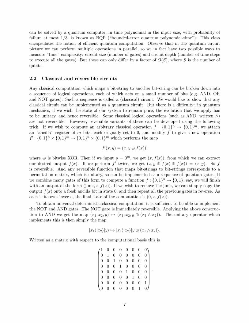
To obtain universal deterministic classical computation, it is sufficient to be able to implementthe NOT and AND gates. The NOT gate is immediately reversible. Applying the above construc-tion to AND we get the map (x1, x2, y) 7→ (x1, x2, y ⊕ (x1 ∧ x2)). The unitary operator whichimplements this is then simply the map
|x1〉|x2〉|y〉 7→ |x1〉|x2〉|y ⊕ (x1 ∧ x2)〉.
Written as a matrix with respect to the computational basis this is
1 0 0 0 0 0 0 00 1 0 0 0 0 0 00 0 1 0 0 0 0 00 0 0 1 0 0 0 00 0 0 0 1 0 0 00 0 0 0 0 1 0 00 0 0 0 0 0 0 10 0 0 0 0 0 1 0
,
7

an operation known as the Toffoli gate. In a circuit diagram, the Toffoli gate is written as“controlled-controlled-NOT”, i.e.
••
It is known that the Toffoli gate, together with the Hadamard gate, are even sufficient for universalquantum computation. Another representative universal set of quantum gates is H,X,CNOT, T,where T =
(1 00 eiπ/4
).
Randomised classical computation can also be embedded in a quantum circuit. Imagine wehave a classical computation which makes use of some random bits, each of which is 0 or 1 withequal probability. We can simulate this by applying a Hadamard gate to |0〉 to produce the state
1√2(|0〉 + |1〉). Then we can either measure this qubit immediately to obtain a uniformly random
bit, or if we prefer, apply classical gates to it and then measure it at the end of the computation;the result is the same.
2.3 Query complexity
While time complexity is a practically important measure of the complexity of algorithms, it suffersfrom the difficulty that it is very hard to prove lower bounds on it, and that technical details cansometimes obscure the key features of an algorithm. One way to sidestep this is to use a model whichis less realistic, but cleaner and more mathematically tractable: the model of query complexity.
In this model, we assume we have access to an oracle, or “black box”, to which we can passqueries, and which returns answers to our queries. Our goal is to determine some property of theoracle using the minimal number of queries. On a classical computer, we can think of the oracle asa function f : 0, 1n → 0, 1m. We pass in inputs x ∈ 0, 1n, and receive outputs f(x) ∈ 0, 1m.How does this fit into physical reality? We imagine we are given access to the oracle either as aphysical device which we cannot open and look inside, or as a circuit which we can see, but forwhich it might be difficult to compute some property of the circuit. For example, even given adescription of a circuit computing some function f : 0, 1n → 0, 1, it might be hard to find aninput x such that f(x) = 1. Sometimes it is more natural to think of an oracle function f as amemory storing n strings of m bits each, where we can retrieve an arbitrary string at the cost ofone query.
We can give a quantum computer access to a oracle using the standard reversible computationconstruction discussed in the previous section. That is, instead of having a function f : 0, 1n →0, 1m, we produce a unitary operator Of which performs the map
Of |x〉|y〉 = |x〉|y ⊕ f(x)〉.
If m = 1, so f returns one bit, it would also make sense to consider an oracle Uf which does notuse an ancilla, but instead flips the phase of an input state |x〉 by applying the map
Uf |x〉 = (−1)f(x)|x〉.
This variant is thus sometimes known as the phase oracle. Given access to a bit oracle, we cansimulate a phase oracle by attaching an ancilla qubit in the state 1√
2(|0〉 − |1〉):
Of |x〉1√2
(|0〉 − |1〉) =1√2
(|x〉|f(x)〉 − |x〉|f(x)⊕ 1〉) = (−1)f(x)|x〉 1√2
(|0〉 − |1〉).
8

Note that the ancilla qubit is left unchanged by this operation, which is called the phase kickbacktrick. Also note that the effect of the phase oracle is not observable if we apply it to just one basisstate |x〉, but only if we apply it to a superposition:∑
x∈0,1nαx|x〉 7→
∑x∈0,1n
(−1)f(x)αx|x〉.
Importantly, note that to implement the oracles Of and Uf we do not need to understand anymore about the inner workings of f than we do classically. That is, if we are given a classicalcircuit computing f , we can follow a purely mechanical construction to create quantum circuitsimplementing Of and Uf .
9

3 Grover’s algorithm
A simple example of a problem that fits into the query complexity model is unstructured search ona set of N elements (Box 2).
In the unstructured search problem, we are given access to a function f : [N ] → 0, 1with the promise that f(x0) = 1 for a unique element x0. Our task is to output x0.
Box 2: Unstructured search for a unique marked element
It is intuitively clear that the unstructured search problem should require about N queries tobe solved (classically!). We can formalise this as the following proposition:
Proposition 3.1. Let A be a classical algorithm which solves the unstructured search problem on aset of N elements with failure probability δ < 1/2. Then A makes Ω(N) queries in the worst case.
Proof sketch. We can think of any classical algorithm A as choosing in advance, either determinis-tically or randomly, a sequence S of distinct indices x1, . . . , xN to query, and then querying themone by one. Imagine an adversary chooses the marked element x0 uniformly at random. Then,on average, x0 will appear at position N/2 in the sequence S. As for a random choice of x0 thealgorithm makes Ω(N) queries on average, the average number of queries made in the worst casemust also be Ω(N).
In the quantum setting, we will see that the unstructured search problem can be solved withsignificantly fewer queries.
Theorem 3.2 (Grover ’97). There is a quantum algorithm which solves the unstructured searchproblem using O(
√N) queries.
For simplicity, assume that N = 2n for some integer n (this is not an essential restriction).Then Grover’s algorithm is described in Box 3.
We are given access to f : 0, 1n → 0, 1 with the promise that f(x0) = 1 for a uniqueelement x0. We use a quantum circuit on n qubits with initial state |0〉⊗n. Let H denotethe Hadamard gate, and let U0 denote the n-qubit operation which inverts the phase of|0〉: U0|0〉 = −|0〉, U0|x〉 = |x〉 for x 6= 0.
1. Apply H⊗n.
2. Repeat the following operations T times, where T = bπ4√Nc:
(a) Apply Uf .
(b) Apply D := −H⊗nU0H⊗n.
3. Measure all the qubits and output the result.
Box 3: Grover’s algorithm
The overall unitary operation performed is thus (−H⊗nU0H⊗nUf )TH⊗n, where T = bπ4
√Nc.
(Incidentally, note that the minus sign in front of D can actually be omitted without affecting the
10

correctness of the algorithm, but it is helpful for the analysis.) In circuit diagram form, Grover’salgorithm looks like this:
|0〉 H
Uf D Uf
. . .
D|0〉 H . . .
......
|0〉 H . . .
It may be far from clear initially why this algorithm works, or indeed whether it does work. Todescribe the algorithm, we introduce unitary operators I|ψ〉 and R|ψ〉, where |ψ〉 is an arbitrarystate. These are defined as follows:
I|ψ〉 := I − 2|ψ〉〈ψ|, R|ψ〉 := −I|ψ〉 = 2|ψ〉〈ψ| − I,
where I is the identity. I|ψ〉 can be seen as an “inversion about |ψ〉” operation, while R|ψ〉 can beseen as an “reflection about |ψ〉” operation. An arbitrary state |φ〉 can be expanded as
|φ〉 = α|ψ〉+ β|ψ⊥〉
for some α and β, and some state |ψ⊥〉 such that 〈ψ|ψ⊥〉 = 0. Then
I|ψ〉|φ〉 = −α|ψ〉+ β|ψ⊥〉,
so I|ψ〉 has flipped the phase of the component corresponding to |ψ〉, and left the componentorthogonal to |ψ〉 unchanged. R|ψ〉 has the opposite effect. Observe that, in the unstructuredsearch problem with marked element x0, Uf = I|x0〉. Further observe that
H⊗nU0H⊗n = H⊗n(I − 2|0〉〈0|)H⊗n = I − 2|+〉〈+| = I|+〉,
where |+〉 = 1√2n
∑x∈0,1n |x〉, so D = −I|+〉. By moving the minus sign, the algorithm can equally
well be thought of as alternating the operations −I|x0〉 and I|+〉, or equivalently R|x0〉 and −R|+〉.We have the following claims:
1. For any states |ψ〉, |φ〉, and any state |ξ〉 in the 2d plane spanned by |ψ〉 and |φ〉, the statesR|ψ〉|ξ〉 and R|φ〉|ξ〉 remain in this 2d plane.
This is immediate from geometric arguments, but one can also calculate explicitly:
R|ψ〉(α|ψ〉+ β|φ〉) = R|ψ〉(α|ψ〉+ β(γ|ψ〉+ δ|ψ⊥〉)) = (α+ βγ)|ψ〉 − βδ|ψ⊥〉= (α+ 2βγ)|ψ〉 − β(γ|ψ〉+ δ|ψ⊥〉) = (α+ 2βγ)|ψ〉 − β|φ〉.
2. Within the 2d plane spanned by orthogonal states |ψ〉, |ψ⊥〉, I|ψ〉 = −R|ψ〉 = R|ψ⊥〉 .
Again, one can calculate explicitly that
−R|ψ〉(α|ψ〉+ β|ψ⊥〉) = −α|ψ〉+ β|ψ⊥〉 = R|ψ⊥〉(α|ψ〉+ β|ψ⊥〉).
3. If |ξ〉 is within the 2d plane spanned by |ψ〉, |ψ⊥〉,
R|ψ〉|ξ〉 = 〈ψ|ξ〉|ψ〉 − 〈ψ⊥|ξ〉|ψ⊥〉.
This is just a straightforward calculation.
11

Combining these claims, we see that each step of Grover’s algorithm consists of two reflectionsin the plane spanned by |+〉, |x0〉: a reflection about |x0〉 followed by a reflection about |+⊥〉,a state orthogonal to |+〉 within this plane. We can illustrate this with the following diagram,demonstrating the effect of these operations on an arbitrary state |ξ〉 within this 2d plane:
|+〉
|x0〉|+⊥〉|ξ〉 R|x0〉 R|+⊥〉
|+〉
|x0〉|+⊥〉
|ξ〉
|+〉
|x0〉|+⊥〉|ξ〉
We see that |ξ〉 has moved closer to |x0〉. In fact, geometrically speaking, the composition oftwo reflections is a rotation! If the angle between |ξ〉 and |x0〉 is θ, and the angle between |x0〉and |+⊥〉 is γ, composing these two reflections rotates |ξ〉 in the direction of |+⊥〉 by an angle of2θ − 2(θ − γ) = 2γ. This is proven by picture in the following diagram but could also be shownusing the representation of rotations and reflections by 2d matrices.
|+〉
|x0〉|+⊥〉|ξ〉
θ
γR|x0〉 R|+⊥〉
|+〉
|x0〉|+⊥〉
|ξ〉θγ
|+〉
|x0〉|+⊥〉|ξ〉θ − 2γ
Repeating the Grover iteration continues to rotate |ξ〉 within this plane by angle 2γ. We stopwhen we are as close to |x0〉 as possible. We start with |ξ〉 = |+〉, so the initial angle between|ξ〉 and |x0〉 is π/2 − γ. We can calculate what γ is by using the formula cos γ = 〈x0|+⊥〉, sosin γ = 〈x0|+〉 = 1/
√N . As sinx ≈ x for small x, we expect the number of iterations required to
move from an angle of π/2−γ down to an angle of 0 to be about (π/4)√N . One can calculate this
more precisely: after T iterations, the angle between |ξ〉 and |x0〉 is
γT := π/2− (2T + 1) arcsin(1/√N),
so the probability of obtaining the outcome x0 when we measure is precisely
|〈ξ|x0〉|2 = cos2(γT ) = sin2((2T + 1) arcsin(1/√N)). (1)
Maximising this by taking T to be the integer nearest to
π
4 arcsin(1/√N)− 1
2=π
4
√N − 1
2−O
(1
N
),
we learn x0 with probability 1 − O(1/N) using O(√N) queries. (The above expression uses
arcsinx = x + O(x3) for small x.) Figure 4 illustrates the success probabilities for N = 100.
12

T
Success probability
1
10 20 30 40 50
Figure 4: Success probabilities of Grover’s algorithm for N = 100.
We see that, as the number of uses of the Grover iterate increases past (π/4)√N , the success
probability starts to decrease. This is sometimes referred to as the “souffle” property of Grover’salgorithm: if we open the oven too early, or too late, the souffle falls.
A particularly nice case, where we can determine an exact solution, is N = 4. Here we havearcsin(1/2) = π/6, so if we plug in T = 1 to Eqn. (1), the probability of getting the outcome x0 issin2(π/2) = 1; so we get the right answer with certainty after only one query.
We have calculated the query complexity of Grover’s algorithm; what is the time complexity?As well as the calls to Uf , we need to implement the operation D. But this can be done efficiently:D consists of two layers of n Hadamard gates and an operation which flips the phase if the inputis not all 0’s. This operation – which is based on computing the bitwise OR of n bits – can beimplented using O(log n) layers of classical gates. So the overhead is O(n) gates per iteration, anddepth only O(log n). This is minor compared with the number of iterations, which is Θ(2n/2).
3.1 Multiple marked elements
Grover’s algorithm can also be used when there are M > 1 marked elements. In this setting, theoperator Uf inverts the phase of input elements x ∈ S, for some unknown subset S ⊆ [N ], where|S| = M . Uf is still related to an inversion operator, but now an inversion about an M -dimensionalsubspace:
Uf = I − 2ΠS ,
where ΠS =∑
x∈S |x〉〈x|. If we define the state |S〉 := 1√M
∑x∈S |x〉, we see that
I|S〉|+〉 = (I − 2|S〉〈S|)|+〉 = |+〉 − 2
1
M
∑x,y∈S
|x〉〈y|
1√N
∑x∈0,1n
|x〉
= |+〉 − 2√
N
∑x∈S|x〉 = (I − 2ΠS)|+〉 = Uf |+〉
and similarlyI|S〉|S〉 = −|S〉 = (I − 2ΠS)|S〉 = Uf |S〉.
That is, the Uf operation behaves like an inversion-about-|S〉 operator for any states in the subspacespanned by |+〉 and |S〉. The whole of the previous analysis goes through, except that now theangle γ moved at each step satisfies sin γ = 〈S|+〉 =
√M/N . Thus after T iterations we have
|〈ξ|S〉|2 = cos2(γT ) = sin2((2T + 1) arcsin(√M/N)).
13

By a similar argument to before we can pick T ≈ (π/4)√N/M to obtain overlap with |S〉 close
to 1. When we measure at the end of the algorithm, we get an element of the subset S (and infact a uniformly random such element) with probability |〈ξ|S〉|2. In particular, observe that whenM = N/4, we again measure an element of S with certainty using only one query.
What if we do not know the number of marked elements in advance? The following simple trickcan deal with this. First run the algorithm assuming there is 1 marked element; if it fails, try againassuming there are 2 marked elements; then 4, 8, etc. The total number of queries used is roughly
log2N∑k=0
π
4
√N
2k=π
4
√N
logN∑k=0
2−k/2 = O(√N).
If the number of marked elements is M , at least one of the iterations must choose a value of T whichis within a factor of 2 of the optimal value T ′ ≈ (π/4)
√N/M . Then, as (2T ′+1) arcsin(
√M/N) =
π/2 +O(M/N),
sin2((2T + 1) arcsin(√M/N)) = sin2
(2T + 1
2T ′ + 1(2T ′ + 1) arcsin(
√M/N)
)= sin2
(2T + 1
2T ′ + 1(π/2 +O(M/N))
),
which is lower-bounded by a strictly positive constant if M is small with respect to N . Repeatingthe whole algorithm O(1) times allows us to achieve an arbitrarily high success probability.
This algorithm might still have a high probability of failing in the case where M = Ω(N). Tofind a marked element in this case we can just sample O(1) random values of f(x) classically; wewill find a marked element with high probability.
3.2 Problems in NP and “database search”
Grover’s algorithm is often presented as a way of searching an unstructured database, or a databasewhich is not structured in a way that is useful to us; for example, trying to search by phone numberin a phone book ordered by name. However, the primary use of Grover’s algorithm (at least initially)is likely not to be searching physical databases, but instead searching for solutions to computationalproblems.
Grover’s algorithm gives a quadratic quantum speedup over classical exhaustive search for anyproblem in NP. This is because we can choose the oracle operation f to be the classical checkingcircuit which takes an input a claimed solution, and outputs 1 if the solution is correct, and 0otherwise. If there are N possible solutions to the problem, Grover’s algorithm lets us find asolution using only O(
√N) checks. Note that this does not immediately imply that Grover’s
algorithm is better than any classical algorithm; in some cases, there could be a more efficientclassical algorithm based on using the structure of the problem.
But could we also use Grover’s algorithm to search a real database? This would rely on the useof a “quantum RAM” which allowed elements of the memory to be efficiently queried in superpo-sition. In principle, there do not seem any fundamental reasons why such a memory could not beconstructed. However, in practice building a quantum RAM is likely to be challenging.
14

3.3 Amplitude amplification
The basic idea behind Grover’s algorithm can be generalised remarkably far, to an algorithmfor finding solutions to any problem using a heuristic. This algorithm is known as amplitudeamplification.
Imagine we have N possible solutions, of which a subset S are “good”, and we would like to finda good solution. As well as having access to a “checking” algorithm f as before, where f(x) = 1if and only if x is marked, we now have access to a “guessing” algorithm A, which has the job ofproducing potential solutions to the problem. It performs the map
A|0〉 =N−1∑x=0
αx|x〉
for some coefficients αx. So, if we were to apply A and then measure, the probability that wewould obtain a good solution is
p :=∑x∈S|αx|2;
we think of A as a heuristic which tries to output a good solution. We can use f to check whethera claimed solution is actually good. If we repeated Algorithm A until we got a good solution, theexpected number of trials we would need is Θ(1/p).
We now describe the amplitude amplification algorithm.
We are given access to A and Uf as above.
1. Apply A to the starting state |0〉.
2. Repeat the following operations T times, for some T to be determined:
(a) Apply Uf .
(b) Apply −AI0A−1.
3. Measure all the qubits and output the result.
Box 5: Amplitude amplification
Note that this is exactly the same as Grover’s algorithm, except that we have replaced the H⊗n
operations with A or A−1. Write
|ψ〉 = A|0〉, |G〉 =ΠS |ψ〉‖ΠS |ψ〉‖
,
where again ΠS =∑
x∈S |x〉〈x|. We now repeat the analysis of the previous section, except thatwe replace |+〉 with |ψ〉 and |S〉 with |G〉. We observe that everything goes through just as before!The first operation applied is equivalent to I|G〉, and the second is equivalent to −I|ψ〉. We startwith the state |ψ〉 and rotate towards |G〉. The angle γ moved at each step now satisfies
sin γ = 〈ψ|G〉 = ‖ΠS |ψ〉‖ =√p,
so the number of iterations required to move from |ψ〉 to |G〉 is O(1/√p) – a quadratic improvement.
15

Finally observe that we can generalise one step further, by replacing the algorithm Uf withinversion about an arbitrary subspace, rather than a subspace defined in terms of computationalbasis vectors. This allows us to use amplitude amplification to drive amplitude towards an arbitrarysubspace, or indeed to create an arbitrary quantum state, given the ability to reflect about thatstate.
16
7 3 4 2 9 7 3 4 2 9 7 3 4 2 9 7 3 4 2 9
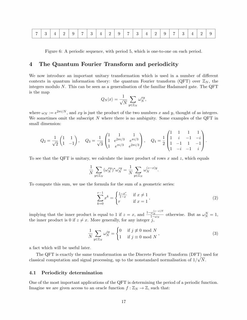
Figure 6: A periodic sequence, with period 5, which is one-to-one on each period.
4 The Quantum Fourier Transform and periodicity
We now introduce an important unitary transformation which is used in a number of differentcontexts in quantum information theory: the quantum Fourier transform (QFT) over ZN , theintegers modulo N . This can be seen as a generalisation of the familiar Hadamard gate. The QFTis the map
QN |x〉 =1√N
∑y∈ZN
ωxyN ,
where ωN := e2πi/N , and xy is just the product of the two numbers x and y, thought of as integers.We sometimes omit the subscript N where there is no ambiguity. Some examples of the QFT insmall dimension:
Q2 =1√2
(1 11 −1
), Q3 =
1√3
1 1 1
1 e2πi/3 eπi/3
1 eπi/3 e2πi/3
, Q4 =1
2
1 1 1 11 i −1 −i1 −1 1 −11 −i −1 i
.
To see that the QFT is unitary, we calculate the inner product of rows x and z, which equals
1
N
∑y∈ZN
(ωxyN )∗ωzyN =1
N
∑y∈ZN
ω(z−x)yN .
To compute this sum, we use the formula for the sum of a geometric series:
r−1∑k=0
xk =
1−xr1−x if x 6= 1
r if x = 1, (2)
implying that the inner product is equal to 1 if z = x, and1−ω(z−x)N
N1−ωN otherwise. But as ωNN = 1,
the inner product is 0 if z 6= x. More generally, for any integer j,
1
N
∑y∈ZN
ωjyN =
0 if j 6≡ 0 mod N
1 if j ≡ 0 mod N, (3)
a fact which will be useful later.
The QFT is exactly the same transformation as the Discrete Fourier Transform (DFT) used forclassical computation and signal processing, up to the nonstandard normalisation of 1/
√N .
4.1 Periodicity determination
One of the most important applications of the QFT is determining the period of a periodic function.Imagine we are given access to an oracle function f : ZN → Z, such that:
17

• f is periodic: there exists r such that r divides N and f(x+ r) = f(x) for all x ∈ ZN ;
• f is one-to-one on each period: for all pairs (x, y) such that |x− y| < r, f(x) 6= f(y).
Our task is to determine r.
The periodicity determination algorithm is presented in Box 7.
We are given access to a periodic function f with period r, which is one-to-one on eachperiod. We start with the state |0〉|0〉.
1. Apply QN to the first register.
2. Apply Of to the two registers.
3. Measure the second register.
4. Apply QN to the first register.
5. Measure the first register; let the answer be k.
6. Simplify the fraction k/N as far as possible and return the denominator.
Box 7: Periodicity determination
The initial sequence of operations which occur during the algorithm is:
|0〉|0〉 17→ 1√N
∑x∈ZN
|x〉|0〉 27→ 1√N
∑x∈ZN
|x〉|f(x)〉.
When the second register is measured, we receive an answer, say z. By the periodic and one-to-oneproperties of f , all input values x ∈ ZN for which f(x) = z are of the form x0 + jr for some x0 andinteger j. The state therefore collapses to something of the form√
r
N
N/r−1∑j=0
|x0 + jr〉.
After we apply the QFT, we get the state
√r
N
N/r−1∑j=0
∑y∈ZN
ωy(x0+jr)N |y〉
=
√r
N
∑y∈ZN
ωyx0
N/r−1∑j=0
ωjryN
|y〉.Observe that, as r divides N , ωrN = e2πi(r/N) = ωN/r. This state is thus equivalent to
√r
N
∑y∈ZN
ωyx0
N/r−1∑j=0
ωjyN/r
|y〉.By Eqn. (3), the sum over j is 0 unless y ≡ 0 mod N/r, or in other words if y = `N/r for someinteger `. So we can rewrite this state as
1√r
r−1∑`=0
ω`x0N/r|`N/r〉.
18

0 2 4 6 8 10 12 14 16 18
0.25
0 2 4 6 8 10 12 14 16 18
0.25
Figure 8: Periodicity determination as above with N = 20, r = 5. First diagram illustrates theprobabilities of measurement outcomes after step 3 (for one possible measurement result for thesecond register), second diagram illustrates probabilities after step 5.
When we perform the final measurement, we receive an outcome k = `0N/r, for some `0 pickeduniformly at random from 0, . . . , r − 1. We know that
k =`0N
r, so
k
N=`0r.
In this equation, we know N and k and would like to determine r. If it happened that `0 werecoprime to r, we could cancel the fraction on the left-hand side and output the denominator. Whatis the probability that we are lucky in this way?
Fact 4.1. Fix an positive integer a and pick b uniformly at random from the integers between 0and a. Then the probability that b is coprime to a is Ω(1/ log log a).
Thus, if we repeat the whole procedure O(log log r) = O(log logN) times, we are quite likely tofind the period r. Why? If we have a probabilistic procedure which succeeds with probability p,the probability that it fails every time over R repetitions is exactly
(1− p)R ≤ e−pR,
so it suffices to take R = O(1/p) to achieve, say, 99% success probability. Each time the algorithmreturns a claimed period, we can check whether it is really a period of the function using twoadditional queries. Each use of the quantum algorithm therefore makes 3 queries, so the wholealgorithm makes O(log logN) queries in total. In terms of time complexity, the most complicatedclassical processing required is the elementary arithmetic in step 6, which can be implemented (viaEuclid’s algorithm) using poly(logN) arithmetic operations. However, we have not yet shown thatwe can implement the QFT QN efficiently.
4.2 Efficient implementation of the QFT
We will show here how to implement QN efficiently – i.e. using a circuit of size O(poly logN) –in the case where N is a power of 2. (In fact, the QFT can also be implemented (approximately)efficiently when N is not a power of 2.) The efficient implementation is based on the same ideasas the classical Fast Fourier Transform (FFT). To begin with, we observe that the output of theQFT, when applied to a computational basis state, has an efficient description as a product state.
Assume that N = 2n for some integer n, and represent each y ∈ ZN by the n-bit string
19

(y0, y1, . . . , yn−1), where y = y0 + 2y1 + 4y2 + · · ·+ 2n−1yn−1. Then
QN |x〉 =1
2n/2
∑y∈Z2n
ωxy2n |y〉
=1
2n/2
∑y∈0,1n
ωx(
∑n−1j=0 2jyj)
2n |yn−1〉|yn−2〉 . . . |y0〉
=
1√2
∑yn−1∈0,1
ω2n−1xyn−1
2n |yn−1〉
1√2
∑yn−2∈0,1
ω2n−2xyn−2
2n |yn−2〉
. . .
1√2
∑y0∈0,1
ωxy02n |y0〉
=
n⊗j=1
1√2
∑yn−j∈0,1
ωxyn−j2j
|yn−j〉
.
Because xyn−j ≡ 0 mod 2j when x is an integer multiple of 2j , we see that the j’th qubit of theoutput only depends on the j bits x0, . . . , xj−1. We can write this another way, as
QN |x〉 =1
2n/2
(|0〉+ e2πi(.x0)|1〉
)(|0〉+ e2πi(.x1x0)|1〉
). . .(|0〉+ e2πi(.xn−1...x0)|1〉
),
where the notation (.xj . . . x0) is used for the binary fraction
xj2
+xj−1
4+ . . .
x0
2j−1.
So we see that the first qubit of the output depends on only the last qubit of the input, the secondqubit depends on the last two, etc. We can utilise this structure by building up the output statein reverse order. The last stage of the circuit creates the correct state for the first qubit, which isthen not used again; the last but one stage creates the correct state for the second qubit, etc. Toproduce the correct state for each qubit, we can use the gates H and Rd, where
H =1√2
(1 11 −1
), Rd =
(1 0
0 eπi/2d
).
Here we are assuming that we have access to Rd gates for arbitrary d; as briefly discussed in Section2, this is not essential as any universal gate set will allow us to approximately implement thesegates. Observe that the Hadamard gate can be written as the map
H|x〉 =1√2
(|0〉+ e2πi(.x)|1〉
)for x ∈ 0, 1. We can use this to start building up a binary fraction in the phase of the basisstate |1〉. Applying a Rd gate to this state will add 1/2d+1 to this binary fraction. To apply Rdconditional on the bits of x, we will use controlled-Rd gates.
The easiest way to illustrate this process is with an example. The overall circuit for the QFTon 4 qubits can be depicted as
|x3〉 H R1 R2 R3 |y0〉
|x2〉 • H R1 R2 |y1〉
|x1〉 • • H R1 |y2〉
|x0〉 • • • H |y3〉
20

Observe that the output state is backwards, i.e. the qubits appear in reverse order. They can bereturned to the original order, if desired, using swap gates. How many gates in total are used inthe circuit? The j’th stage of the circuit, for j = 1, . . . , n, uses one Hadamard gate and n − j Rdgates. Thus the overall number of gates used is O(n2); n(n−1)/2 Rd gates and n Hadamard gates,then n additional swap gates, if used. This is O(log2N), so we have indeed obtained an efficientcircuit.
This complexity can be improved further, to O(n log n), if we are content with an approximateversion of the QFT. The observation which implies this is that many of the operations in the circuitare Rd gates for large values of d, which do not affect the output significantly. Indeed, it turns outthat there is a constant C such that if we omit the gates Rd with d ≥ C log n, for any input state|x〉 the output is close to the input up to an error of at most 1/poly(n). The modified circuit usesO(log n) gates at each stage, so O(n log n) in total.
21

5 Integer factorisation
The main application of periodicity determination is Shor’s quantum algorithm for integer factori-sation. Given an n-digit integer N as input, this algorithm outputs a non-trivial factor of N (or thatN is prime, if this is the case) with success probability 1− ε, for any ε > 0, in time O(n3). The best
classical algorithm known (the general number field sieve) runs in time eO(n1/3 log2/3 n). In fact, thisis a heuristic bound and this algorithm’s worst-case runtime has not been rigorously determined;the best proven bound is somewhat higher. Shor’s algorithm thus achieves a super-polynomialimprovement. This result might appear only of mathematical interest, were it not for the fact thatthe widely-used RSA public-key cryptosystem relies on the hardness of integer factorisation. Shor’sefficient factorisation algorithm implies that this cryptosystem is insecure against attack by a largequantum computer.
Unfortunately (?), proving correctness of Shor’s algorithm requires going through a number oftechnical details. First we need to show that factoring reduces to a periodicity problem – though inthis case an approximate periodicity problem. This part uses only classical number theory. Then weneed to show that periodicity can still be determined even in the setting where the input functionis only approximately periodic. This part uses the theory of continued fractions.
5.1 From factoring to periodicity
The basic skeleton of the quantum factorisation algorithm is given in Box 9. It is based on two“magic” subroutines. The first is a classical algorithm for computing the greatest common divisor(gcd) of two integers. This can be achieved efficiently using Euclid’s algorithm. The second ingre-dient is an algorithm for computing the order of an integer a modulo N , i.e. the smallest integer rsuch that ar ≡ 1 mod N ; this is where we will use periodicity determination. As long as a and Nare coprime, such an integer p exists:
Fact 5.1 (Euler’s theorem). If a and N are coprime then there exists p such that ar ≡ 1 mod N .
Let N denote the integer to be factorised. Assume that N is not even or a power of aprime.
1. Choose 1 < a < N uniformly at random.
2. Compute b = gcd(a,N). If b > 1 output b and stop.
3. Determine the order r of a modulo N . If r is odd, the algorithm has failed; termi-nate.
4. Compute s = gcd(ar/2 − 1, N). If s = 1, the algorithm has failed; terminate.
5. Output s.
Box 9: Integer factorisation algorithm (overview)
We start by showing that this algorithm does work, assuming that the subroutines used allwork correctly. If a is coprime to N , there exists r such that ar ≡ 1 mod N . If, further, such an ris even, we can factor
ar − 1 = (ar/2 + 1)(ar/2 − 1) ≡ 0 mod N.
22

So N divides the product (ar/2 + 1)(ar/2− 1). Because r is the smallest integer x such that ax ≡ 1mod N , we know that ar/2− 1 is not divisible by N . Then, if in addition s = gcd(ar/2− 1, N) 6= 1,s would be a nontrivial factor of N . This condition would hold if ar/2 + 1 is not divisible by N .This, and r being even, turn out to occur with quite high probability:
Fact 5.2. Let N be odd and not a power of a prime. If 1 < a < N is chosen uniformly at randomwith gcd(a,N) = 1, then Pr[r is even and ar/2 6≡ −1 mod N ] ≥ 1/2.
The algorithm thus succeeds with probability at least 1/2. If it fails, we simply repeat thewhole process. After K repetitions, we achieve a failure probability of at most 1/2K . Even if theorder-finding procedure has some small probability of error (which will turn out to be the case),we can check whether the algorithm’s output s is correct by attempting to divide N by s.
We assumed throughout that N is not even or a power of a prime. If N is even, we simplyoutput 2 as a factor. To deal with the case that N = p` for some prime p and some integer ` > 0,we observe that we can efficiently compute the roots N1/k, for k = 2, . . . , log2N . If any of these isan integer, we have found a factor of N . Finally, what about if N is itself prime? In this case thealgorithm will fail every time. We can therefore output “prime” after a suitable number of failures.
Example 5.3. Consider N = 15. Imagine we choose a = 7 at random. Then gcd(7, 15) = 1.The function f(x) = 7x mod 15 takes values 1, 7, 4, 13, 1, . . . for x ≥ 0. So r = 4 and we have(72 + 1)(72 − 1) ≡ 0 mod 15. The greatest common divisor of 72 − 1 = 48 and 15 is 3, which isindeed a factor of 15.
It remains to show how to implement step 3. Consider the function f : Z→ ZN defined by
f(x) = ax mod N.
We have f(x + y) = f(x)f(y) and, by Euler’s theorem, f(r) = 1. So f(x + r) = f(x)f(r) = f(x)for all x, i.e. f is periodic with period r. Since r is the smallest integer such that f(r) = 1, we alsohave that f is one-to-one on each period. However, although this function is periodic on the wholedomain Z, we will need to truncate it to a finite size. If we knew what the period was, we couldchoose this size to make the function periodic again, but of course we do not know this in advance.This will lead to the function becoming no longer exactly periodic, but just approximately periodic.
5.2 Approximate periodicity
We restrict the function f(x) = ax mod N to the set x ∈ 0, . . . ,M − 1, where M = 2m is thesmallest power of 2 greater than N2 (we will see the reasons behind this choice later). WriteM = Br + b for 0 ≤ b < r, where B = bM/rc. That is, the function is periodic up to the lastperiod, which is truncated and contains only b elements, rather than r. We apply the steps of theperiodicity-determination algorithm to f as in Section 4.1. That is, we first construct the state
1√M
M−1∑x=0
|x〉|f(x)〉,
then measure the second register to receive an answer z = f(x0) for some x0. The state of the firstregister then becomes
|ψ〉 =1√A
A−1∑j=0
|x0 + jr〉,
23

0 2 4 6 8 10 12 14 16 18 20 22 24 26 28 30
0.2
Figure 10: The probabilities of different measurement outcomes for a function with period 5, withM = 32. Note the peaks around multiples of 32/5 = 6.4.
where A = B + 1 if x0 < b, and A = B if x0 ≥ b. Write
QM |ψ〉 =
M−1∑y=0
αy|y〉
for the resulting state when we apply the QFT to |ψ〉. By direct calculation we have
αy =1√MA
A−1∑j=0
ωy(x0+jr)M =
ωyx0M√MA
A−1∑j=0
(ωyrM)j.
Using the formula (2) for the sum of a geometric series, the sum evaluates to
1− ωyrAM
1− ωyrM
if yr 6≡ 0 mod M , and evaluates to A otherwise. Previously, in the case of exact periodicitydetermination, we had A = B = M/r, so the numerator was 0 unless yr 6≡ 0 mod M , or in otherwords y is a multiple of M/r. Now we aim to show that, when we measure, we get an outcome ywhich is close to a multiple of the non-integer value M/r with high probability. This situation isillustrated in Figure 10.
When we measure, the probability of obtaining outcome y is
Pr[y] =1
MA
∣∣∣∣∣1− ωyrAM
1− ωyrM
∣∣∣∣∣2
=1
MA
∣∣∣∣∣1− e2πiyrA/M
1− e2πiyr/M
∣∣∣∣∣2
=sin2(πyrA/M)
MA sin2(πyr/M).
To see the third equality, note that |1 − eiθ| = |eiθ/2 − e−iθ/2| = 2| sin(θ/2)| for any real θ. Nowconsider values y of the form y = b`M/re for some integer `. We can write any such integer asy = `M/r + ε for some small ε such that |ε| ≤ 1/2. Indeed, we have the slightly stronger bound(which we will need) that |ε| ≤ 1/2− 1/r. This holds because (a) `M/r is an integer divided by r,so the distance from the closest integer is an multiple of 1/r; (b) r < N and M > N2 is a powerof 2, so any factors of 2 in the denominator of the fraction `M/r can be cancelled and we cannothave |ε| = 1/2.
Then
Pr[y] =sin2(π(`M/r + ε)rA/M)
MA sin2(π(`M/r + ε)r/M)=
sin2(`Aπ + εrAπ/M)
MA sin2(`π + εrπ/M)=
sin2(εrAπ/M)
MA sin2(εrπ/M)
24

by periodicity of the function | sin θ|. We now claim (see (4) in Box 11) that the following pair ofinequalities hold for any θ in the range 0 ≤ θ ≤ π/2:
(2/π)θ ≤ sin θ ≤ θ.
Assuming these inequalities, we have
Pr[y] ≥ (2εrA/M)2
MA(εrπ/M)2=
4A
π2M≥ 4
π2M
(M
r− 1
)=
4
π2r−O(1/N2).
Note that the lower bound on the numerator is valid because |ε|rAπ/M ≤ π/2, which was aconsequence of |ε| ≤ 1/2− 1/r:
|ε|rAπM
≤(
12 −
1r
)r(Mr + 1
)π
M=π
2
(1− 2
r
)(1 +
r
M
)≤ π
2
(1− 2
r
)(1 +
2
r
)=π
2
(1− 4
r2
)<π
2,
where the second inequality holds because r2 ≤ N2 ≤ 2M . Therefore, as there are r “good” integersy of the form b`M/rc, the probability of obtaining at least one of them is at least 4/π2 −O(1/N).
The following trigonometric inequalities will be useful for the analysis of various quantumalgorithms. We state them without proof, instead referring to the figure below.
(2/π)θ ≤ sin θ ≤ θ for 0 ≤ θ ≤ π/2; (4)
cos θ ≥ 1− θ2/2 for all θ. (5)
sin θ
(2/π)θ
θπ/2
π/4
π/2π/4
cos θ
1− θ2/2
1
0.5
π/2π/4
Box 11: Trigonometric inequalities
5.3 Learning r from an approximate period
It remains to extract r from an integer y of the form y = b`M/re. Divide y by M to obtain arational number z such that ∣∣∣∣ `r − z
∣∣∣∣ < 1
2M<
1
2N2.
We would like to find the fraction `/r from z. We first claim that there is at most one fraction ofthe form `′/r′ with r′ < N satisfying the above bound. To prove this, imagine there were two suchfractions `′/r′, `′′/r′′. Then ∣∣∣∣ `′r′ − `′′
r′′
∣∣∣∣ =|`′r′′ − r′`′′|
r′r′′≥ 1
r′r′′>
1
N2.
But, as `′/r′, `′′/r′′ are each within 1/(2N2) of z, they must be at most distance 1/N2 apart, sowe have a contradiction.
25

We have seen that it suffices to find any fraction `′/r′ such that r′ < N to learn `/r. To dothis, we use the theory of continued fractions. The continued fraction expansion (CFE) of z is anexpression of the form
z =1
a1 + 1a2+ 1
a3+...
,
where the ai are positive integers. To find the integers ai, we start by writing
z =1
z′,
where z′ = a1 + b for some integer a1 and some b < 1; then repeating this process on b. Notethat, for any rational z, this expansion must terminate after some number of iterations C. One canshow that in fact, for any rational z = s/t where s and t are m-bit integers, C = O(m). Once wehave calculated this expansion, if we truncate it after some smaller number of steps, we obtain anapproximation to z. These approximations are called convergents of the CFE.
Example 5.4. The continued fraction expansion of z = 31/64 is
31
64=
1
2 + 115+ 1
2
.
The convergents are1
2,
1
2 + 115
=15
31.
Fact 5.5. Any fraction p/q with |p/q − z| < 1/(2q2) will appear as one of the convergents of theCFE of z.
Therefore, if we carry out the continued fraction expansion of z, we are guaranteed to find `/r,as the unique fraction close enough to z.
Example 5.6. Imagine we want to factor N = 21. We set M = 512 > 212 and choose a = 10 atrandom. The order of a mod 21 is 6. So we would expect the measurement outcomes we receiveto be close to multiples of 512/6 = 851
3 . Imagine we receive a measurement result of 427. This isa “good” result, as the closest integer to 5× (512/6) = 4262
3 . The continued fraction expansion ofz = 427/512 is
427
512=
1
1 + 15+ 1
42+12
.
From this we obtain the sequence of convergents
1,1
1 + 15
=5
6,
1
1 + 15+ 1
42
=211
253.
Only the second of these has a denominator smaller than N and is within 1/(2N2) of z. Therefore,we have `/r = 5/6. We output the denominator, 6, as our guess for the period r. . . which is correct!
26

5.4 Complexity analysis
How complex is the final, overall algorithm? Recall that N is n bits in length. We have seen thatthe QFT on ZM can be implemented in time O(log2M) = O(n2). To implement the modularexponentiation operation f(x) = ax mod N efficiently, we can use repeated squaring to producef(2k) for any integer k in k squaring operations. Multiplying the different values f(2k) togetherfor each k such that the k’th bit of a is nonzero produces f(x). So we require O(n) multiplicationsof n-bit integers to compute f(x). Multiplying two n-bit numbers can be achieved classically usingstandard long multiplication in time O(n2), so we get an overall complexity of O(n3).
It turns out (though we will not show it here) that the classical processing of the measurementresults based on Euclid’s algorithm and the continued fractions algorithm can also be done in timeO(n3). Thus the overall time complexity of the whole algorithm is O(n3), whereas the best knownclassical algorithm runs in time exponential in n1/3. The asymptotic quantum complexity can infact be improved a bit further, to O(n2 poly log n), by using more advanced multiplication anddivision algorithms with runtime O(n poly log n). However, these algorithms only become moreefficient in practice for very large values of n.
27

6 Phase estimation
We now discuss an important primitive used in quantum algorithms called phase estimation, whichprovides a different and unifying perspective on the quantum algorithms which you have just seen.Phase estimation is once again based on the QFT over ZN , where N = 2n.
Imagine we are given a unitary operator U . U may either be written down as a quantum circuit,or we may be given access to a black box which allows us to apply a controlled-U j operation forinteger values of j. We are also given a state |ψ〉 which is an eigenvector of U : U |ψ〉 = e2πiφ|ψ〉 forsome real φ such that 0 ≤ φ < 1. We would like to determine φ to n bits of precision, for somearbitrary n.
To do so, we prepend an n qubit register to |ψ〉, initially in the state |0〉, and create the state
1√N
N−1∑x=0
|x〉|ψ〉
by applying Hadamards to each qubit in the first register. We then apply the unitary operator
U ′ =N−1∑x=0
|x〉〈x| ⊗ Ux.
This operator can be described as: if the first register contains x, apply U x times to the secondregister. We are left with the state
1√N
N−1∑x=0
e2πiφx|x〉|ψ〉;
note that the second register is left unchanged by this operation. We now apply the operator Q−1
to the first register and then measure it, receiving outcome x (say). We output the binary fraction
0.x1x2 . . . xn =x1
2+x2
4+ · · ·+ xn
2n
as our guess for φ. The following is an explicit circuit for the above algorithm.
|0〉 H . . . •
Q−1
......
|0〉 H • . . .
|0〉 H • . . .
|ψ〉 U20 U21 . . . U2n−1
Why does this algorithm work? When we perform the final measurement, the probability of gettingthe outcome x is
1
N2
∣∣∣∣∣∣N−1∑y=0
e2πiφy−2iπxy/N
∣∣∣∣∣∣2
=1
N2
∣∣∣∣∣∣N−1∑y=0
e2πiy(φ−x/N)
∣∣∣∣∣∣2
.
28

First imagine that the binary expansion of φ is at most n bits long, or in other words φ = z/N forsome 0 ≤ z ≤ N − 1. In this case we have
1
N2
∣∣∣∣∣∣N−1∑y=0
e2πiy(φ−x/N)
∣∣∣∣∣∣2
=1
N2
∣∣∣∣∣∣N−1∑y=0
e2πiy(z−x)/N
∣∣∣∣∣∣2
= δxz
by the unitarity of the QFT, so the measurement outcome is guaranteed to be z, implying thatthe algorithm outputs φ with certainty. If the binary expansion of φ is longer than n bits, we nowshow that we still get the best possible answer with probability Ω(1), and indeed are very likelyto get an answer close to φ. The proof turns out to be very similar to that of correctness of theperiodicity determination algorithm in the approximate case.
Theorem 6.1. The probability that the above algorithm outputs the real number with n binarydigits which is closest to φ is at least 4/π2. Further, the probability that the algorithm outputs θsuch that |θ − φ| ≥ ε is at most O(1/(Nε)).
Proof. If the binary expansion of φ has n binary digits or fewer, we are done by the argumentabove. So, assuming it does not, let φ be the closest approximation to φ that has n binary digits,and write φ = a/N for some integer 0 ≤ a ≤ N−1. For any z, define δ(z) := φ−z/N and note that0 < |δ(a)| ≤ 1/(2N). For any φ, the probability of getting outcome z from the final measurementis
Pr[z] =1
N2
∣∣∣∣∣∣N−1∑y=0
e2πiy(φ−z/N)
∣∣∣∣∣∣2
=1
N2
∣∣∣∣∣∣N−1∑y=0
e2πiyδ(z)
∣∣∣∣∣∣2
=1
N2
∣∣∣∣∣1− e2πiNδ(z)
1− e2πiδ(z)
∣∣∣∣∣2
=sin2(πNδ(z))
N2 sin2(πδ(z)),
(6)where we evaluate the sum using the formula for a geometric series. This quantity should befamiliar from the proof of correctness of the periodicity determination algorithm.
We first lower bound this expression for z = a to prove the first part of the lemma. As|δ(a)| ≤ 1/(2N), we have Nπδ(a) ≤ π/2. Then
Pr[a] =sin2(πNδ(a))
N2 sin2(πδ(a))≥ (2Nδ(a))2
N2(πδ(a))2=
4
π2
using the trigonometric inequalities (4).
In order to prove the second part of the theorem, we now find an upper bound on expression(6). First, it is clear that sin2(πNδ(z)) ≤ 1 always. For the denominator, by the same argumentto above we have sin(πδ(z)) ≥ 2δ(z) and hence, for all z,
Pr[get outcome z] ≤ 1
N2
(1
2δ(z)
)2
=1
4N2δ(z)2.
We now sum this expression over all z such that |δ(z)| ≥ ε. The sum is symmetric about δ(z) = 0,and as z is an integer, the terms in this sum corresponding to δ(z) > 0 are δ0, δ0 + 1/N, . . . , forsome δ0 ≥ ε. The sum will be maximised when δ0 = ε, when we obtain
Pr[get outcome z with |δ(z)| ≥ ε] ≤ 1
4N2
∞∑k=0
1
(ε+ k/N)2≤ 1
4
∫ ∞0
1
(Nε+ k)2dk
=1
4
∫ ∞Nε
1
k2dk = O
(1
Nε
).
29
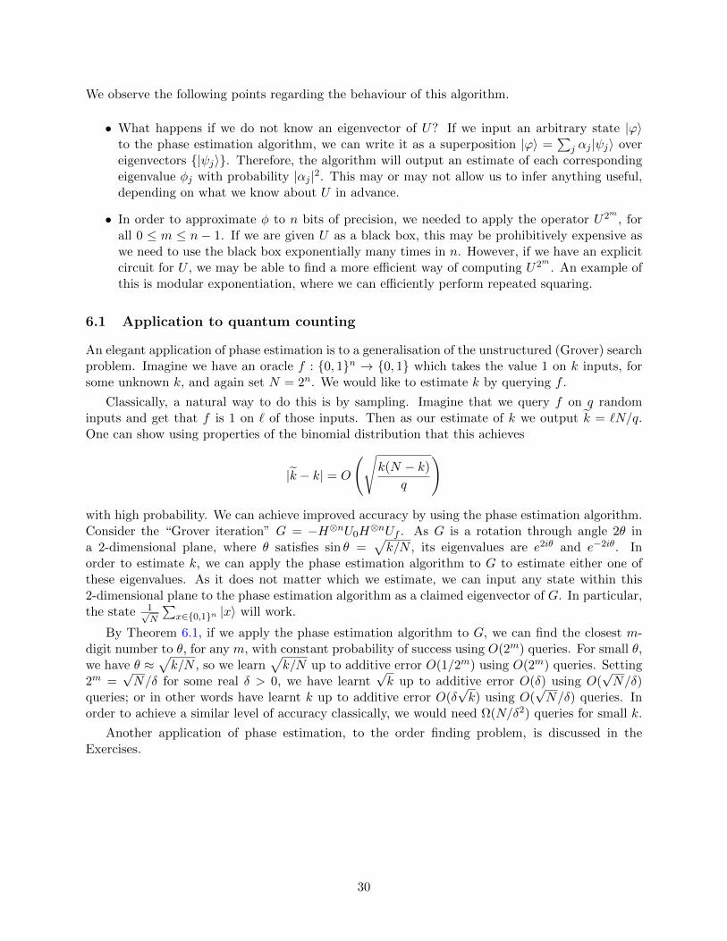
We observe the following points regarding the behaviour of this algorithm.
• What happens if we do not know an eigenvector of U? If we input an arbitrary state |ϕ〉to the phase estimation algorithm, we can write it as a superposition |ϕ〉 =
∑j αj |ψj〉 over
eigenvectors |ψj〉. Therefore, the algorithm will output an estimate of each correspondingeigenvalue φj with probability |αj |2. This may or may not allow us to infer anything useful,depending on what we know about U in advance.
• In order to approximate φ to n bits of precision, we needed to apply the operator U2m , forall 0 ≤ m ≤ n− 1. If we are given U as a black box, this may be prohibitively expensive aswe need to use the black box exponentially many times in n. However, if we have an explicitcircuit for U , we may be able to find a more efficient way of computing U2m . An example ofthis is modular exponentiation, where we can efficiently perform repeated squaring.
6.1 Application to quantum counting
An elegant application of phase estimation is to a generalisation of the unstructured (Grover) searchproblem. Imagine we have an oracle f : 0, 1n → 0, 1 which takes the value 1 on k inputs, forsome unknown k, and again set N = 2n. We would like to estimate k by querying f .
Classically, a natural way to do this is by sampling. Imagine that we query f on q randominputs and get that f is 1 on ` of those inputs. Then as our estimate of k we output k = `N/q.One can show using properties of the binomial distribution that this achieves
|k − k| = O
(√k(N − k)
q
)
with high probability. We can achieve improved accuracy by using the phase estimation algorithm.Consider the “Grover iteration” G = −H⊗nU0H
⊗nUf . As G is a rotation through angle 2θ ina 2-dimensional plane, where θ satisfies sin θ =
√k/N , its eigenvalues are e2iθ and e−2iθ. In
order to estimate k, we can apply the phase estimation algorithm to G to estimate either one ofthese eigenvalues. As it does not matter which we estimate, we can input any state within this2-dimensional plane to the phase estimation algorithm as a claimed eigenvector of G. In particular,the state 1√
N
∑x∈0,1n |x〉 will work.
By Theorem 6.1, if we apply the phase estimation algorithm to G, we can find the closest m-digit number to θ, for any m, with constant probability of success using O(2m) queries. For small θ,we have θ ≈
√k/N , so we learn
√k/N up to additive error O(1/2m) using O(2m) queries. Setting
2m =√N/δ for some real δ > 0, we have learnt
√k up to additive error O(δ) using O(
√N/δ)
queries; or in other words have learnt k up to additive error O(δ√k) using O(
√N/δ) queries. In
order to achieve a similar level of accuracy classically, we would need Ω(N/δ2) queries for small k.
Another application of phase estimation, to the order finding problem, is discussed in theExercises.
30
7 Hamiltonian simulation
One of the earliest – and most important – applications of a quantum computer is likely to bethe simulation of quantum mechanical systems. There are quantum systems for which no efficientclassical simulation is known, but which we can simulate on a universal quantum computer. Whatdoes it mean to “simulate” a physical system? According to the OED, simulation is “the techniqueof imitating the behaviour of some situation or process (whether economic, military, mechanical,etc.) by means of a suitably analogous situation or apparatus”. What we will take simulation tomean here is approximating the dynamics of a physical system. Rather than tailoring our simulatorto simulate only one type of physical system (which is sometimes called analogue simulation), weseek a general simulation algorithm which can simulate many different types of system (sometimescalled digital simulation).
According to the laws of quantum mechanics, time evolution of the state |ψ〉 of a quantumsystem is governed by Schrodinger’s equation:
i~d
dt|ψ(t)〉 = H(t)|ψ(t)〉,
where H(t) is the Hamiltonian of the system (for convenience, we will henceforth absorb ~ intoH(t)). An important special case on which we will focus is the time-independent setting whereH(t) = H is constant. In this case the solution of this equation is
|ψ(t)〉 = e−iHt|ψ(0)〉.
Given a physical system specified by some Hamiltonian H, we would like to simulate the evolutionof the system on an arbitrary initial state for a certain amount of time t. In other words, given H,we would like to implement a unitary operator which approximates
U(t) = e−iHt.
What does it mean to approximate a unitary? The “gold standard” of approximation is approxi-mation in the operator norm (aka spectral norm)
‖A‖ := max|ψ〉6=0
‖A|ψ〉‖‖|ψ〉‖
,
where ‖|ψ〉‖ =√〈ψ|ψ〉 is the usual Euclidean norm of |ψ〉. Note that this is indeed a norm, and
in particular satisfies the triangle inequality ‖A+ B‖ ≤ ‖A‖+ ‖B‖. We say that U approximatesU to within ε if
‖U − U‖ ≤ ε.
This is a natural definition of approximation because it implies that, for any state |ψ〉, U |ψ〉 andU |ψ〉 are only distance at most ε apart.
7.1 Simulation of k-local Hamiltonians
For simplicity, assume that H is a Hamiltonian of n two-level systems (qubits). In order for ourquantum simulation of H to be efficient, we need U = e−iHt to be approximable by a quantumcircuit containing poly(n) gates. A fairly straightforward counting argument shows that not all
31
Hamiltonians H can be simulated efficiently. However, it turns out that several important phys-ically motivated classes can indeed be simulated. Perhaps the most important of these is k-localHamiltonians.
A Hamiltonian H of n qubits is said to be k-local if it can be written as a sum
H =m∑j=1
Hj
for some m, where each Hj is a Hermitian matrix which acts non-trivially on at most k qubits. Thatis, Hj is the tensor product of a matrix H ′j on k qubits, and the identity matrix on the remainingn− k qubits. For example, the operator on 3 qubits
H = X ⊗ I ⊗ I − 2I ⊗ Z ⊗ Y
is 2-local. Many interesting physical systems are k-local for small k (say k ≤ 3), some of which youmay have heard of. Simple examples include the two-dimensional Ising model on a n × n squarelattice,
H = Jn∑
i,j=1
Z(i,j)Z(i,j+1) + Z(i,j)Z(i+1,j)
and the Heisenberg model on a line,
H =
n∑i=1
JxX(i)X(i+1) + JyY
(i)Y (i+1) + JzZ(i)Z(i+1),
both of which are used in the study of magnetism (in the above, M (j) denotes a single qubit operatoracting on the j’th qubit, and J, Jx, Jy, Jz are constants).
Note that, if H is k-local, we can assume that m ≤(nk
)= O(nk). We usually assume that
k is constant, in which case m is polynomial in n. We first show that each of the individual Hj
operators can be simulated efficiently, which will be immediate from the following theorem, whichformalises a claim made at the start of the course.
Theorem 7.1 (Solovay-Kitaev theorem). Let U be a unitary operator which acts non-triviallyon k = O(1) qubits, and let S be an arbitrary universal set of quantum gates. Then U can beapproximated in the operator norm to within ε using O(logc(1/ε)) gates from S, for some c < 4.
Proof. Sadly beyond the scope of this course. For a readable explanation, see Andrew Childs’lecture notes.
As each e−iHjt acts non-trivially on only at most k qubits, it follows from the Solovay-Kitaev the-orem that we can approximate each of these operators individually to within ε in timeO(polylog(1/ε)).In the special case where all of the Hj operators commute, we have
e−iHt = e−i(∑mj=1Hj)t =
m∏j=1
e−iHjt.
Thus a natural way to find a unitary operator approximating e−iHt is to take the product of ourapproximations of e−iH1t, . . . , e−iHmt. Although each of these approximates e−iHjt to within ε, thisdoes not imply that their product approximates e−iHt to within ε. However, we now show that theapproximation error only scales linearly.
32

Lemma 7.2. Let (Ui), (Vi) be sequences of m unitary operators satisfying ‖Ui − Vi‖ ≤ ε for all1 ≤ i ≤ m. Then ‖Um . . . U1 − Vm . . . V1‖ ≤ mε.
Proof. The proof is by induction on m. The claim trivially holds for m = 1. Assuming that itholds for a given m, we have
‖Um+1Um . . . U1 − Vm+1Vm . . . V1‖= ‖Um+1Um . . . U1 − Um+1Vm . . . V1 + Um+1Vm . . . V1 − Vm+1Vm . . . V1‖≤ ‖Um+1Um . . . U1 − Um+1Vm . . . V1‖+ ‖Um+1Vm . . . V1 − Vm+1Vm . . . V1‖= ‖Um+1(Um . . . U1 − Vm . . . V1)‖+ ‖(Um+1 − Vm+1)Vm . . . V1‖= ‖Um . . . U1 − Vm . . . V1‖+ ‖Um+1 − Vm+1‖≤ (m+ 1)ε.
Thus, in order to approximate∏mj=1 e
−iHjt to within ε, it suffices to approximate each of theHj to within ε/m. We formalise this as the following proposition.
Proposition 7.3. Let H be a Hamiltonian which can be written as the sum of m commuting termsHj, each acting non-trivially on k = O(1) qubits. Then, for any t, there exists a quantum circuitwhich approximates the operator e−iHt to within ε in time O(m polylog(m/ε)).
7.2 The non-commuting case
Unfortunately, this simulation technique does not necessarily work for non-commuting Hj . The rea-son is that if A and B are non-commuting operators, it need not hold that e−i(A+B)t = e−iAte−iBt.However, we can simulate non-commuting Hamiltonians via an observation known as the Lie-Trotterproduct formula.
In what follows, the notation X +O(ε), for a matrix X, is used as shorthand for X +E, whereE is a matrix satisfying ‖E‖ ≤ Cε, for some universal constant C (not depending on X or ε).
Lemma 7.4 (Lie-Trotter product formula). Let A and B be Hermitian matrices such that ‖A‖ ≤ Kand ‖B‖ ≤ K, for some real K ≤ 1. Then
e−iAe−iB = e−i(A+B) +O(K2).
Proof. From the Taylor series for ex, for any matrix A such that ‖A‖ = K ≤ 1, we have
e−iA = I − iA+
∞∑k=2
(−iA)k
k!= I − iA+ (−iA)2
∞∑k=0
(−iA)k
(k + 2)!= I − iA+O(K2).
Hence
e−iAe−iB =(I − iA+O(K2)
) (I − iB +O(K2)
)= I − iA− iB +O(K2) = e−i(A+B) +O(K2).
33

Applying this formula multiple times, for any Hermitian matrices H1, . . . ,Hm satisfying ‖Hj‖ ≤K ≤ 1 for all j,
e−iH1e−iH2 . . . e−iHm =(e−i(H1+H2) +O(K2)
)e−iH3 . . . e−iHm
=(e−i(H1+H2+H3) +O((2K)2)
)e−iH4 . . . e−iHm +O(K2)
= e−i(H1+···+Hm) +O(K2) +O((2K)2) + · · ·+O(((m− 1)K)2)
= e−i(H1+···+Hm) +O(m3K2).
Therefore, there is a universal constant C such that if n ≥ Cm3(Kt)2/ε,∥∥∥e−iH1t/ne−iH2t/n . . . e−iHmt/n − e−i(H1+···+Hm)t/n∥∥∥ ≤ ε/n.
By Lemma 7.2, for any such n∥∥∥(e−iH1t/ne−iH2t/n . . . e−iHmt/n)n− e−i(H1+···+Hm)t
∥∥∥ ≤ ε.Given this result, we can simulate a k-local Hamiltonian simply by simulating the evolution ofeach term for time t/n to high enough accuracy and concatenating the individual simulations. Weformalise this as the following theorem.
Theorem 7.5. Let H be a Hamiltonian which can be written as the sum of m terms Hj, each actingnon-trivially on k = O(1) qubits and satisfying ‖Hj‖ ≤ K for some K. Then, for any t, there existsa quantum circuit which approximates the operator e−iHt to within ε in time O(m3(Kt)2/ε), up topolylogarithmic factors.
It seems somewhat undesirable that, in order to simulate a Hamiltonian for time t, this algorithmhas dependence on t which is O(t2). In fact, using more complicated simulation techniques, theoverall complexity in Theorem 7.5 can be improved to time O(mKt), up to polylogarithmic factors.
34
8 Quantum walk
We now discuss a quantum generalisation of the classical concept of random walk. Classically,random walks are an important algorithmic tool, and the same has proven to be true for quantumwalks. We begin by introducing the most basic variant of quantum walk, walk on the line.
8.1 Quantum walk on the line
Classically, the simple random walk on the line is defined as follows. A particle (“walker”) is placedon an infinite line at position 0. At each time step, the walker flips an unbiased coin. If the result isheads, it moves left by 1; otherwise, it moves right by 1. The probability of being found at positionx after t steps is exactly
1
2t
(tt+x
2
),
where we define(tr
)= 0 for non-integer r. (This is easily derived as follows: there are 2t different
paths of n steps that could be taken; the paths which end up at x are exactly those with (t+ x)/2right-moving steps; and there are
(t
(t+x)/2
)such paths.) We can see from this that the probability
decays quickly for |x| outside the range O(√t), and indeed one can calculate the variance of the
position p as
E[p2] = E
( t∑i=1
Zi
)2 =
t∑i,j=1
E[ZiZj ] =
t∑i=1
E[Z2i ] = t,
where the Zi ∈ ±1 are random variables determining whether the i’th step is to the left or theright. We look for a quantum generalisation of this simple process.
One natural generalisation is as follows. Consider a quantum system with two registers |x〉|c〉,where the first holds an integer position1 x and the second holds a coin state c ∈ L,R. As in theclassical case, at each step our quantum walk will flip a coin and then decide in which direction tomove. These two operations will be unitary: a coin operator C, and a shift operator S. The coinoperator acts solely on the coin register, and consists of a Hadamard operation:
C|L〉 =1√2
(|L〉+ |R〉) , C|R〉 =1√2
(|L〉 − |R〉) .
The shift operator acts on both registers, and simply moves the walker in the direction indicatedby the coin state:
S|x〉|L〉 = |x− 1〉|L〉, S|x〉|R〉 = |x+ 1〉|R〉.
Then a quantum walk on the line for t steps consists of applying the unitary operator (S(I⊗C))t tosome initial state. Remarkably, these simple dynamics can lead to some fairly complicated results.Consider the first few steps of a quantum walk with initial state |0〉|L〉 (position 0, facing left).
1The reader might object to a register that stores an arbitrary integer. In this case, consider it to store an integermod m for some large m.
35

One can calculate that the state evolves as follows.
|0〉|L〉 7→ 1√2
(|−1〉|L〉+ |1〉|R〉)
7→ 1
2(|−2〉|L〉+ |0〉|R〉+ |0〉|L〉 − |2〉|R〉)
7→ 1
2√
2(|−3〉|L〉+ |−1〉|R〉+ 2|−1〉|L〉 − |1〉|L〉+ |3〉|R〉)
7→ . . .
Consider the result of measuring the position register after the third step. Positions −3, 1 and 3are obtained with probability 1/8 each, and position −1 is obtained with probability 5/8. In otherwords, the most likely position for the particle to be found in is −1. By contrast, the classicalrandom walk is symmetric about 0 (and in fact is found in position −3 or 3 with probability 1/8each, and −1 and 1 with probability 3/8 each). The bias of the quantum walk is an effect ofinterference. If the quantum walk is run for more steps before measuring the position, we obtainthe pattern illustrated in Figure 12.
-100 -90 -80 -70 -60 -50 -40 -30 -20 -10 0 10 20 30 40 50 60 70 80 90 1000
0.02
0.04
0.06
0.08
0.10
0.12
0.14
Figure 12: The distribution of positions following a quantum walk on the line for 100 steps usingthe Hadamard coin. Only even positions are shown as the amplitude at odd positions is 0.
Note that, unlike the classical walk, the quantum walk is not symmetric about 0. Intuitively,this is caused by the Hadamard coin treating the L and R directions differently: only the |R〉state gets mapped to a state containing a negative amplitude, leading to destructive interferencein this direction. This asymmetry can be removed by changing the initial state of the coin registerto 1√
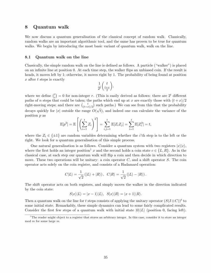
2|0〉(|L〉 + i|R〉), or alternatively by using a different coin operator. Figure 13 compares the
distribution of probabilities obtained for classical and (symmetric) quantum walks.
The quantum walk seems to spread out from the origin faster than the classical walk. Indeed,it can be shown that the variance is Ω(t2), noticeably faster than the classical O(t). Unlike thestraightforward analysis of the classical random walk, the effect of interference means that it is quiteinvolved to prove this, so we will not do so here. This difference between quantum and classicalwalks will become more pronounced when we consider more general graphs.
36
-100 -90 -80 -70 -60 -50 -40 -30 -20 -10 0 10 20 30 40 50 60 70 80 90 1000
0.01
0.02
0.03
0.04
0.05
0.06
0.07
0.08
Figure 13: Quantum walk on the line for 100 steps with starting coin state 1√2|0〉(|L〉 + i|R〉),
compared with classical walk for 100 steps (red dashed line). Only even positions are shown as theamplitude at odd positions is 0.
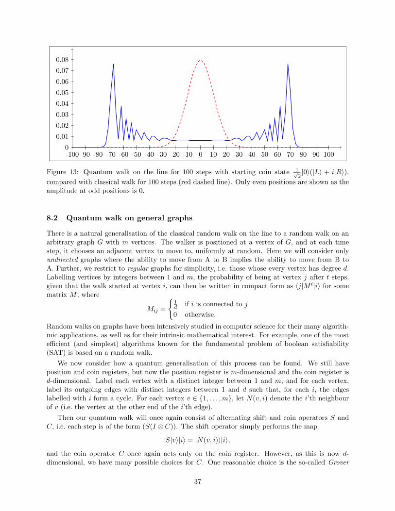
8.2 Quantum walk on general graphs
There is a natural generalisation of the classical random walk on the line to a random walk on anarbitrary graph G with m vertices. The walker is positioned at a vertex of G, and at each timestep, it chooses an adjacent vertex to move to, uniformly at random. Here we will consider onlyundirected graphs where the ability to move from A to B implies the ability to move from B toA. Further, we restrict to regular graphs for simplicity, i.e. those whose every vertex has degree d.Labelling vertices by integers between 1 and m, the probability of being at vertex j after t steps,given that the walk started at vertex i, can then be written in compact form as 〈j|M t|i〉 for somematrix M , where
Mij =
1d if i is connected to j
0 otherwise.
Random walks on graphs have been intensively studied in computer science for their many algorith-mic applications, as well as for their intrinsic mathematical interest. For example, one of the mostefficient (and simplest) algorithms known for the fundamental problem of boolean satisfiability(SAT) is based on a random walk.
We now consider how a quantum generalisation of this process can be found. We still haveposition and coin registers, but now the position register is m-dimensional and the coin register isd-dimensional. Label each vertex with a distinct integer between 1 and m, and for each vertex,label its outgoing edges with distinct integers between 1 and d such that, for each i, the edgeslabelled with i form a cycle. For each vertex v ∈ 1, . . . ,m, let N(v, i) denote the i’th neighbourof v (i.e. the vertex at the other end of the i’th edge).
Then our quantum walk will once again consist of alternating shift and coin operators S andC, i.e. each step is of the form (S(I ⊗ C)). The shift operator simply performs the map
S|v〉|i〉 = |N(v, i)〉|i〉,
and the coin operator C once again acts only on the coin register. However, as this is now d-dimensional, we have many possible choices for C. One reasonable choice is the so-called Grover
37
coin,
C =
2d − 1 2
d . . . 2d
2d
2d − 1 . . . 2
d...
.... . .
...2d
2d . . . 2
d − 1
.
This is just the iteration used in Grover’s algorithm. This operator is an appealing choice because itis permutation-symmetric (i.e. treats all edges equally), and it is far away from the identity matrix(i.e. has a large mixing effect). If d = 2, we would get C = ( 0 1
1 0 ), so in this case the coins usedearlier for the walk on the line lead to more interesting behaviour.
8.3 Exponentially faster hitting on the hypercube
We now focus on one particularly interesting graph: the n-dimensional hypercube (aka the Cayleygraph of the group Zn2 ). This is the graph whose vertices are n-bit strings which are adjacent ifthey differ in exactly one bit. Each edge x ↔ y of this graph is naturally labelled by the indexof the single bit where x and y differ. We will be interested in the expected time it takes for arandom walk on this graph to travel from the “all zeroes” string 0n to the “all ones” string 1n, i.e.to traverse the graph from one extremity to the other, which is known as the hitting time from 0n
to 1n.
Classically, this time can be analysed by mapping the walk to a (biased) random walk on theline. Imagine the walker is currently at a vertex with Hamming weight k. The probability ofmoving to a vertex with Hamming weight (k− 1) is k/n, and the probability of moving to a vertexwith Hamming weight (k + 1) is 1 − k/n. Observe that, as k increases, the probability of a stepleading to the Hamming weight increasing decreases, so intuitively the walker becomes “stuck” inthe “middle” of the graph (i.e. near Hamming weight n/2).
More rigorously, we have the following proposition.
Proposition 8.1. The hitting time from 0n to 1n is at least 2n − 1.
Proof. Let h(k) be the expected number of steps until the walk hits 1n, given that it starts withHamming weight k. We have the recurrence
h(k) =k
nh(k − 1) +
(1− k
n
)h(k + 1) + 1,
with the boundary case h(n) = 0. Writing δ(k) = h(k)− h(k + 1), this can be simplified to
δ(k) =
(n
k + 1− 1
)δ(k + 1)− n
k + 1
and the recurrence solved to give
δ(k) =1(n−1k
) k∑j=0
(n
j
), and hence h(0) =
n−1∑k=0
δ(n) =
n−1∑k=0
1(n−1k
) k∑j=0
(n
j
).
Thus h(0) can be lower bounded by rearranging the sum to give
h(0) =
n−1∑j=0
(n
j
) n−1∑k=j
1(n−1k
) ≥ n−1∑j=0
(n
j
)= 2n − 1.
38

We thus see that the expected time to reach the 1n vertex is exponential in n. However, forquantum walks the situation is very different, and we have the following result.
Theorem 8.2. If a quantum walk on the hypercube is performed for T ≈ π2n steps starting in
position 0n, and the position register is measured, the outcome 1n is obtained with probability1−O(polylog(n)/n).
Once again, the proof of this result is too technical to include here. However, we can give asketch of the first part of one proof strategy, which is analogous to the classical case, and consists ofsimplifying to a walk on the line. Define a set of 2n states |υk, L〉, |υk, R〉 indexed by an integerk = 0, . . . , n as follows:
|υk, L〉 :=1√k(nk
) ∑x,|x|=k
∑i,xi=1
|x〉|i〉, |υk, R〉 :=1√
(n− k)(nk
) ∑x,|x|=k
∑i,xi=0
|x〉|i〉,
with the exception of the special cases |υ0, L〉 and |υn, R〉, which will not be used and are undefined.Now observe that the quantum walk on the hypercube preserves tbe subspace spanned by this setof states:
S|υk, L〉 =1√k(nk
) ∑x,|x|=k
∑i,xi=1
|x⊕ ei〉|i〉 =1√k(nk
) ∑x,|x|=k−1
∑i,xi=0
|x〉|i〉 = |υk−1, R〉,
and similarly S|υk, R〉 = |υk+1, L〉. In the case of the coin operator, it turns out that
(I ⊗ C)|υk, L〉 =
(2k
n− 1
)|υk, L〉+
2√k(n− k)
n|υk, R〉
and (I ⊗ C)|υk, R〉 =2√k(n− k)
n|υk, L〉+
(1− 2k
n
)|υk, R〉.
This behaviour is similar to the quantum walk on the line, with two differences: first, the directionin which the walker is moving flips with each shift, and second, the coin is different at each position(i.e. depends on k). Based on this reduction, it is easy to plot the behaviour of this quantum walknumerically for small n, as shown in Figure 14.
8.4 A general approach for quantising Markov chains
The method described in the previous section, suitably generalised, allows us to define a quantumwalk on any undirected graph. However, we now describe a different approach, due to Szegedy,which simultaneously allows us to handle directed graphs, and allows us to analyse the propertiesof the quantum walk produced.
In the most general setting, a random walk on a directed graph G with n vertices is describedby an N ×N matrix P with non-negative entries such that
∑Ni=1 Pij = 1 for all j (such matrices
are called stochastic). Pij is the probability of moving to vertex i from vertex j. The quantum walkcorresponding to P is a unitary operation WP on CN ⊗ CN . We can think of this as operating ona space spanned by edges of the graph G. To define WP , we first introduce states
|ψj〉 :=N∑i=1
√Pij |j〉|i〉
39

0 2 4 6 8 10 12 14 16 18 20 22 24 26 28 30 32 34 36 38 40 42 44 46 48 500
0.05
0.1
0.15
0.2
0.25
0.3
0.35
Figure 14: Quantum walk on a 50-dimensional hypercube for 60 steps starting in state |υ0, R〉,compared with classical walk for 1000 steps (red dashed line). Graph plots probability of being ata point with Hamming weight k. Only even positions are shown as the amplitude at odd positionsis 0.
for j = 1, . . . , N . As P is stochastic, these are all normalised states. Write
Π :=N∑j=1
|ψj〉〈ψj |
for the projector onto the subspace spanned by |ψj〉, and let S =∑N
i,j=1 |ij〉〈ji| be the operatorthat swaps the two registers. Then a step of the quantum walk is the unitary operator
WP = S(2Π− I).
2Π−I is a reflection about the subspace spanned by |ψj〉. If P is a random walk on a regular graphwith uniform probability of moving to each neighbour, following this procedure gives a quantumwalk as described in the previous section using the Grover coin. We now analyse the eigenvaluesof WP .
Theorem 8.3. For any N ×N stochastic matrix P , let D be the matrix defined by Dij =√PijPji.
Then, for each eigenvalue λ of D, WP has eigenvalues λ ± i√
1− λ2 = e±i arccosλ. WP also haseigenvalues ±1.
Proof. Set T :=∑N
j=1 |ψj〉〈j|, and for each eigenvector |λ〉 of D, let |λ〉 = T |λ〉. T is an isometry:
T †T =N∑
j,k=1
|j〉〈ψj |ψk〉〈k| =N∑
j,k,`,m=1
√P`jPmk〈j|k〉〈`|m〉|j〉〈k| =
N∑j,`=1
P`j |j〉〈j| = I.
On the other hand,
TT † =
N∑j,k=1
|ψj〉〈j|k〉〈ψk| =N∑j=1
|ψj〉〈ψj | = Π
and finally
T †ST =
N∑j,k=1
|j〉〈ψj |S|ψk〉〈k| =N∑
j,k,`,m=1
√P`jPmk〈j, `|S|k,m〉|j〉〈k| =
N∑j,k=1
√PjkPkj |j〉〈k| = D.
40

If we apply WP to |λ〉, we get
WP |λ〉 = S(2Π− I)|λ〉 = S(2TT † − I)T |λ〉 = S(2T − T )|λ〉 = S|λ〉,
and if we apply WP again we get
WPS|λ〉 = S(2TT † − I)ST |λ〉 = (2STD − T )|λ〉 = (2λS − I)|λ〉.
So WP preserves the subspace spanned by |λ〉, S|λ〉, implying that there is an eigenvector of WP
within this subspace. Let|µ〉 = |λ〉 − νS|λ〉
for some µ ∈ C chosen such that |µ〉 is indeed an eigenvector of WP . Then
WP |µ〉 = S|λ〉 − µ(2λS − I)|λ〉 = µ|λ〉+ (1− 2λµ)S|λ〉,
so for |µ〉 to be an eigenvector we must have
(1− 2λµ) = µ(−µ), so µ2 − 2λµ+ 1 = 0
and hence µ = λ± i√
1− λ2. Finally, for any vector orthogonal to all the states |ψj〉, WP simplyacts as −S, which has eigenvalues ±1.
The matrix D occurring in this theorem is like a “symmetrised” version of P . If P is alreadysymmetric, D = P .
8.5 Search by quantum walk
A natural use for random, or quantum walks, on graphs is search. Imagine that a set S of k verticesare marked. A natural approach to find a marked vertex is to start with some arbitrary vertex,then perform a random walk according to P until we find a marked vertex, when we stop. Thisprocess can be modelled by modifying the initial matrix P to produce a new matrix P ′ where
P ′ij =
1 if i = j and j ∈ S0 if i 6= j and j ∈ SPij otherwise.
Assume that P is symmetric and let PS be the matrix obtained by deleting all the rows and columnsof P corresponding to vertices in S. P ’s largest eigenvalue is 1; let the second largest, in absolutevalue, be 1− δ. δ is known as the spectral gap of P .
We first calculate a bound on the largest eigenvalue of PS .
Lemma 8.4. If the second largest eigenvalue of P , in absolute value, is at most 1− δ and k = εN ,then ‖PS‖ ≤ 1− δε.
Proof. Consider the principal eigenvector |v〉 ∈ RN−k of PS , and let |w〉 ∈ RN be the vectorproduced by adding zeroes at positions corresponding to the marked vertices. We perform theeigendecomposition of P ,
P =N∑i=1
λi|λi〉〈λi|
41
where λ1 = 1, and compute
〈v|PS |v〉 = 〈w|P |w〉 =
N∑i=1
λi|〈λi|w〉|2 = |〈λ1|w〉|2 +
N∑i=2
λi|〈λi|w〉|2
≤ |〈λ1|w〉|2 + (1− δ)N∑i=2
|〈λi|w〉|2
= 1− δN∑i=2
|〈λi|w〉|2
= 1− δ(1− |〈λ1|w〉|2).
Observe that, as P is symmetric, |λ1〉must actually be the uniform superposition |λ1〉 = 1√N
∑Ni=1 |i〉.
Then, if we expand |w〉 =∑
i/∈S αi|i〉, we have
|〈λ1|w〉|2 =1
N
∣∣∣∣∣∑i/∈S
αi
∣∣∣∣∣2
≤ N − |S|N
(∑i/∈S
|αi|2)
=N − kN
= 1− ε,
where the inequality is Cauchy-Schwarz. Hence ‖PS‖ ≤ 1− δε as claimed.
We now describe an algorithm which uses a quantum walk to solve the more restricted problemof distinguishing between the case where there are no marked vertices, and the case where there areεN marked vertices. The algorithm applies phase estimation to the operator WP ′ using as inputthe state
|ψ〉 =1√
N − k
∑j /∈S
|ψj〉,
the uniform superposition over non-marked vertices. This state can be prepared by starting withthe uniform superposition over all vertices, then applying the isometry T , and measuring whetherthe first register corresponds to a marked vertex. If so, we are done; if not, we have prepared|ψ〉. Assuming without loss of generality that the last k elements of [N ] are marked, the matrix Dcorresponding to the walk P ′ is
D =
(PS 00 I
),
so by Theorem 8.3 the eigenvalues of WP ′ are ±1 and e±i arccosλ for each eigenvalue λ of PS . IfS = ∅, then PS = P ′ = P and |ψ〉 is an eigenvector of WP with eigenvalue 1. So phase estimationwill return a phase of 0. On the other hand, if S 6= ∅, |ψ〉 is contained entirely within the subspacecorresponding to the PS block, in which WP ′ has eigenvalues e±i arccosλ. We have
cos θ ≥ 1− θ2/2
for any θ, so arccosλ ≥√
2(1− λ). By Lemma 8.4, the phase of each eigenvalue is at least√
2δεin absolute value.
So, using phase estimation, it suffices to make O(1/√δε) steps of the quantum walk to distin-
guish between the two cases that (a) there are no marked elements, and (b) there are k = εNmarked elements. One might wonder what the point of all this work was, when Grover’s algo-rithm solves the unstructured search problem with an ε fraction of marked elements using O(1/
√ε)
queries, which is faster. The point is that, unlike Grover’s algorithm, the quantum walk algorithm
42
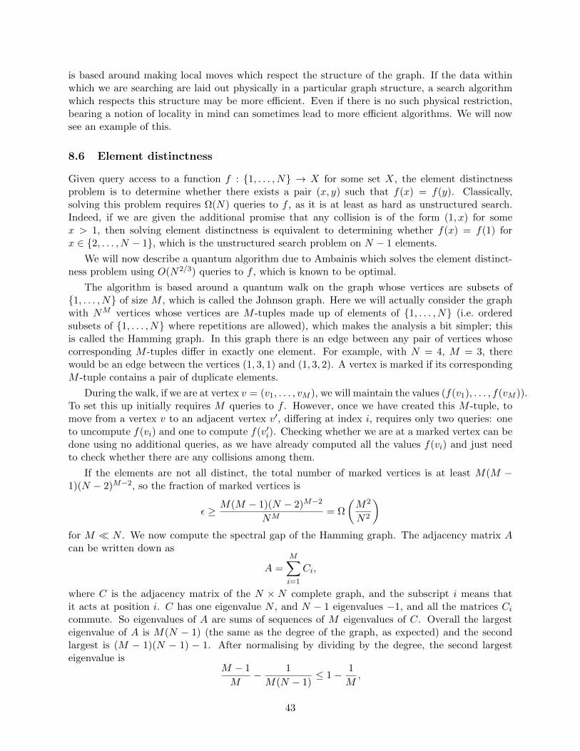
is based around making local moves which respect the structure of the graph. If the data withinwhich we are searching are laid out physically in a particular graph structure, a search algorithmwhich respects this structure may be more efficient. Even if there is no such physical restriction,bearing a notion of locality in mind can sometimes lead to more efficient algorithms. We will nowsee an example of this.
8.6 Element distinctness
Given query access to a function f : 1, . . . , N → X for some set X, the element distinctnessproblem is to determine whether there exists a pair (x, y) such that f(x) = f(y). Classically,solving this problem requires Ω(N) queries to f , as it is at least as hard as unstructured search.Indeed, if we are given the additional promise that any collision is of the form (1, x) for somex > 1, then solving element distinctness is equivalent to determining whether f(x) = f(1) forx ∈ 2, . . . , N − 1, which is the unstructured search problem on N − 1 elements.
We will now describe a quantum algorithm due to Ambainis which solves the element distinct-ness problem using O(N2/3) queries to f , which is known to be optimal.
The algorithm is based around a quantum walk on the graph whose vertices are subsets of1, . . . , N of size M , which is called the Johnson graph. Here we will actually consider the graphwith NM vertices whose vertices are M -tuples made up of elements of 1, . . . , N (i.e. orderedsubsets of 1, . . . , N where repetitions are allowed), which makes the analysis a bit simpler; thisis called the Hamming graph. In this graph there is an edge between any pair of vertices whosecorresponding M -tuples differ in exactly one element. For example, with N = 4, M = 3, therewould be an edge between the vertices (1, 3, 1) and (1, 3, 2). A vertex is marked if its correspondingM -tuple contains a pair of duplicate elements.
During the walk, if we are at vertex v = (v1, . . . , vM ), we will maintain the values (f(v1), . . . , f(vM )).To set this up initially requires M queries to f . However, once we have created this M -tuple, tomove from a vertex v to an adjacent vertex v′, differing at index i, requires only two queries: oneto uncompute f(vi) and one to compute f(v′i). Checking whether we are at a marked vertex can bedone using no additional queries, as we have already computed all the values f(vi) and just needto check whether there are any collisions among them.
If the elements are not all distinct, the total number of marked vertices is at least M(M −1)(N − 2)M−2, so the fraction of marked vertices is
ε ≥ M(M − 1)(N − 2)M−2
NM= Ω
(M2
N2
)for M N . We now compute the spectral gap of the Hamming graph. The adjacency matrix Acan be written down as
A =
M∑i=1
Ci,
where C is the adjacency matrix of the N × N complete graph, and the subscript i means thatit acts at position i. C has one eigenvalue N , and N − 1 eigenvalues −1, and all the matrices Cicommute. So eigenvalues of A are sums of sequences of M eigenvalues of C. Overall the largesteigenvalue of A is M(N − 1) (the same as the degree of the graph, as expected) and the secondlargest is (M − 1)(N − 1) − 1. After normalising by dividing by the degree, the second largesteigenvalue is
M − 1
M− 1
M(N − 1)≤ 1− 1
M,
43
so the spectral gap δ = Ω(1/M). So a marked vertex (i.e. pair of equal elements) can be foundusing
M +O
(1√δε
)= M +O
(N√M
)queries. To minimise this, we set M = Θ(N2/3) to achieve an overall complexity of O(N2/3) queries,as claimed.
44

9 Noise and the framework of quantum channels
Not all processes which occur in quantum mechanics are reversible. As a very simple example,consider the operation of throwing away the input state and replacing it with the state |0〉:
|ψ〉 7→ |0〉
for all |ψ〉. This clearly cannot be implemented as a unitary operator. Just as mixed statesgeneralise pure states, we can generalise unitary operations to so-called completely positive trace-preserving (CPTP) maps, also known as quantum channels. These occur throughout quantuminformation theory and are particularly useful for describing noisy operations and decoherence, thebane of quantum computers.
Recall that a mixed state ρ of n qubits, which describes a probabilistic mixture of pure states |ψ〉,is a Hermitian 2n × 2n matrix which is positive semidefinite (all its eigenvalues are non-negative)and has trace 1. What axioms would we like a physically reasonable map (“superoperator”) E ,which takes mixed states to mixed states, to satisfy?
1. E should be linear: E(pρ+ qσ) = p E(ρ) + q E(σ) for all real p, q.
2. E should be trace-preserving: tr E(ρ) = tr ρ.
3. E should preserve positivity: if ρ ≥ 0, then E(ρ) ≥ 0. But there is a further constraint: ifwe apply E to part of an entangled quantum state, the whole state should remain positivesemidefinite. That is, (E ⊗ I)(ρ) ≥ 0 for ρ ≥ 0, where I is the identity map on an arbitrarilylarge ancilla system. This constraint is called complete positivity.
A completely positive, trace-preserving linear map is called a quantum channel.
9.1 Representations of quantum channels
There are a number of ways in which quantum channels can be represented. We describe two here.
We first consider the Kraus (aka “operator-sum”) representation. Here a channel E with inputdimension din and output dimension dout is described by a sequence of dout × din matrices Ek suchthat ∑
k
E†kEk = I.
The effect of E on a state ρ is then
E(ρ) =∑k
EkρE†k.
A trivial example of a channel in Kraus form is the identity channel I(ρ) = ρ, which has one Krausoperator E1 = I. For a product channel E = E1 ⊗ E2, where
E1(ρ) =∑k
E(1)k ρ(E
(1)k )†, E2(σ) =
∑k
E(2)k σ(E
(2)k )†
we have
E(ρ⊗ σ) = E1(ρ)⊗ E2(σ) =
(∑k
E(1)k ρ(E
(1)k )†
)⊗
(∑`
E(2)` σ(E
(2)` )†
)=
∑k,`
(E(1)k ⊗ E
(2)` )(ρ⊗ σ)((E
(1)k )† ⊗ (E
(2)` )†,
45
so E must have Kraus operators which are tensor products of each pair of those of E1 and E2.
We claim that any superoperator in Kraus form obeys our three axioms:
1. E is linear: for any X and Y ,
E(X + Y ) =∑k
Ek(X + Y )E†k =∑k
EkXE†k +
∑k
EkY E†k = E(X) + E(Y ).
2. E is trace-preserving:
tr E(ρ) = tr
(∑k
EkρE†k
)=∑k
tr(EkρE
†k
)=∑k
tr(ρE†kEk
)= tr
(ρ∑k
E†kEk
)= tr ρ,
where in the second and fourth equalities we use linearity of trace, and in the third we useits invariance under cyclic shifts.
3. E is completely positive. Here it is sufficient to show that E ⊗ I maps positive operatorsto positive operators. Let ρ be an arbitrary positive operator on the extended system (withancilla). Then
(E ⊗ I)(ρ) =∑k
(Ek ⊗ I)ρ(E†k ⊗ I).
For this to be positive semidefinite, it is sufficient that for any positive semidefinite ρ and anymatrix M , MρM † is positive semidefinite. This holds because we can expand ρ as a convexcombination of pure states |ψi〉, and
M |ψi〉〈ψi|M † = |ψ′i〉〈ψ′i|
for some (unnormalised) vector |ψ′i〉, which is positive semidefinite.
In fact, it turns out that the equivalence goes the other way too: every quantum channel can bewritten in Kraus form. We omit the proof (see Nielsen & Chuang, Theorem 8.1).
The Kraus representation is not unique. For example, the channels described by pairs of Krausoperators
E1 =1√2
(1 00 1
), E2 =
1√2
(1 00 −1
), and F1 =
(1 00 0
), F2 =
(0 00 1
)have different representations, but are actually the same channel. This can be seen by writingF1 = (E1 + E2)/
√2, F2 = (E1 − E2)/
√2, and calculating
F1ρF†1 + F2ρF
†2 =
(E1 + E2)ρ(E†1 + E†2) + (E1 − E2)ρ(E†1 − E†2)
2= E1ρE
†1 + E2ρE
†2.
Second, we describe the Stinespring representation. In this representation, a channel E fromsystem A to system B, E : B(CdA) → B(CdB ), is described by an isometry from A to the pair ofsystems B and E, V : CdA → CdB ⊗ CdE , such that
E(ρ) = trE(V ρV †).
That is, the channel consists of applying an isometry to ρ, mapping it into a larger-dimensionalspace, then tracing out part of the space. We can think of this picture as modelling the dynamics
46

of an open quantum system, where ρ interacts with the outside environment E, then to calculatethe final state of the system we discard the environment.
Given a Kraus representation of a channel with operators Ek, we can write down a Stinespringrepresentation in a straightforward way:
V =∑k
Ek ⊗ |k〉. (7)
ThenV †V =
∑k,`
E†kE`〈k|`〉 =∑k
E†kEk = I,
so V is indeed an isometry. Further, for any ρ,
trE(V ρV †) =∑k,`
trE [(Ek ⊗ |k〉)ρ(E†` ⊗ 〈`|)] =∑k,`
trE [(Ekρ⊗ |k〉)(E†` ⊗ 〈`|)]
=∑k,`
(EkρE†` )〈`|k〉 =
∑k
EkρE†k,
so this faithfully represents the original channel. Also observe that any isometry V can be decom-posed as in Eqn. (7), so the equivalence goes both ways. As we can think of any isometry as aunitary operator on a larger space, this correspondence implies that any quantum channel can bethought of as unitary evolution of a larger system, followed by tracing out a subsystem.
9.2 Examples of quantum channels
• Unitary evolution is a quantum channel described by one Kraus operator: ρ 7→ UρU †.
• Discarding ρ and replacing it with some state |ψ〉 is a quantum channel. If ρ is d-dimensional,we have d Kraus operators |ψ〉〈k|, k = 1, . . . , d. Then, for any state ρ,
d∑k=1
|ψ〉〈k|ρ|k〉〈ψ| = |ψ〉
(d∑
k=1
〈k|ρ|k〉
)〈ψ| = (tr ρ)|ψ〉〈ψ| = |ψ〉〈ψ|.
• The qubit depolarising channel replaces the input state ρ with the maximally mixed stateI/2, with probability p; with probability 1− p, the input state is unchanged. That is,
ED(ρ) = pI
2+ (1− p)ρ.
This represents a simple form of noise: with probability p, our knowledge of the qubit is com-pletely randomised, and with probability 1−p the qubit is unharmed. The qubit depolarisingchannel has Kraus operators
E1 =√
1− 3p/4I, E2 = (√p/2)X, E3 = (
√p/2)Y, E4 = (
√p/2)Z.
This can be generalised to d dimensions, where we have
ED(ρ) = pI
d+ (1− p)ρ.
47

• The amplitude damping channel models a scenario in quantum optics where a photonmay be lost, with some probability. We imagine that we have a basis |0〉, |1〉 where 0represents “no photon” and 1 represents “photon” (so this is a very simple example of Fockspace). Then the Kraus operators of the amplitude damping channel EAD are
E0 =
(1 00√
1− γ
), E1 =
(0√γ
0 0
)for some γ, which corresponds to the probability of losing a photon. So
EAD(|0〉〈0|) = |0〉〈0|, EAD(|1〉〈1|) = γ|0〉〈0|+ (1− γ)|1〉〈1|
as expected.
• Every measurement is a quantum channel. Imagine we have a projective measurement, i.e.a set of orthogonal projectors Pk such that
∑k Pk = I. Then the probability that we get
outcome k when we perform this measurement on state ρ is trPkρ, and the resulting state ifthis occurs is
ρ′k :=PkρPktr(Pkρ)
.
The Kraus operators of this channel are just the projectors Pk. This is correct because∑k
PkρPk =∑k
tr(Pkρ)PkρPktr(Pkρ)
;
the output state is a probabilistic mixture of the states ρ′k with the correct probabilities.
If we think of a qubit as a point in R3 using the Bloch ball representation, any channel mapping aqubit to a qubit can be thought of as an affine map on this space. That is, if
ρ =I
2+ αxX + αyY + αzZ,
a channel corresponds to an affine map acting on the 3-dimensional vector v = (αx, αy, αz)T , i.e. a
map of the formv 7→ Av + b
for some 3× 3 matrix A and 3-dimensional vector b.
9.3 Master equations
We remark that it is frequently physically reasonable to think of noise as being a continuous processparametrised by a time t. This leads to the concept of Markovian quantum channels (aka “Markovprocesses”). A Markovian channel is a member of a family Et such that
Es+t = Es Et
for all times s, t. This implies thatEt = etL
48

for some superoperator L. If we write ρ(t) = Et(ρ(0)), ddtρ(t) = L(ρ(t)). If we demand that Et is
completely positive for all times t, it can be shown that L satisfies the master equation
L(ρ) = i[ρ,H] +∑α,β
Gα,β(FαρF†β −
1
2F †βFα, ρ+),
where H is a Hamiltonian, G and Fα are matrices defining a decoherence process, and [., .] and., . denote the commutator and anticommutator, respectively (with the subscript + denoting thepositive part of this operator).
The qubit depolarising and amplitude damping channels, for example, are Markovian. However,not all quantum channels are Markovian.
49

10 Quantum error-correction
Modern computer hardware is extremely reliable. Indeed, it can usually be assumed to be error-freefor all intents and purposes1. However, early quantum computing hardware is likely to be far fromreliable. Even worse, efficient quantum algorithms rely on delicate quantum effects (superpositionand entanglement) which must be preserved in the presence of errors. Luckily, it turns out thaterrors can be fought using the notion of quantum error-correcting codes. To understand thesecodes, it is helpful to first consider a basic classical notion of error correction.
Imagine we have a single bit x which we would like to store in a noisy storage device. A naturalmodel for this noise is that each bit stored in the device gets flipped with probability p, for some0 ≤ p ≤ 1, and is left the same with probability 1−p. So if we store x in the device and then read itback later, we get the wrong answer with probability p. One way to improve this works as follows.Instead of just storing x, store the string xxx, i.e. repeat x three times. Then read out each of thebits of the (potentially corrupted) string to get y := y1y2y3, and output 0 if the majority of thebits of y are 0, and 1 otherwise.
What is the probability of failing to output x if this strategy is followed? The wrong answer willbe returned if two or more of the bits of y are flipped by noise, which will occur with probability3p2(1− p) + p3 = p2(3− 2p) = O(p2). Thus, if p is small, this strategy has improved our resistanceto noise. Indeed, for any p such that 0 < p < 1/2, we have
p2(3− 2p) < p,
so the probability of error has been reduced. Another way of looking at this situation is that wehave stored a bit in such a way that it is impervious to an error affecting a single bit in the storagedevice. The map x 7→ xxx is a very simple example of an error correcting code known as the binaryrepetition code of length 3.
10.1 Quantum errors and error-correction
We would like to find a quantum analogue of this notion of error correction. Rather than preservingclassical bits x, our quantum error correcting code should preserve a qubit |ψ〉 under some notionof error. For the time being, we pretend that an error affecting one or more qubits is simply anarbitrary and unknown unitary operator N applied to those qubits. The classical bit-flip errordiscussed above is an example of this, as it can be seen as simply applying the operator X toa qubit in a computational basis state (recall that X|0〉 = |1〉 and X|1〉 = |0〉). The process ofcorrecting errors in a qubit state |ψ〉 can be written diagrammatically as
|ψ〉E N D
|ψ′〉|0n〉
for some unitary encoding operation E, noise operation N , and decoding operation D. In otherwords, we encode some qubit state |ψ〉 as a larger state |E(ψ)〉 using some ancilla qubits (initiallyin the state |0n〉), some noise is applied, and later we decode the noisy encoded state to produce astate |ψ′〉. The goal is that after this process |ψ′〉 ≈ |ψ〉 for some set of correctable noise operationsN .
There are two obvious ways in which the classical repetition code could be translated to thequantum regime, both of which unfortunately do not work. First, we could measure |ψ〉 in the
1Software, of course, is another matter.
50

computational basis to obtain a bit 0 or 1, then just encode this with the classical repetition code.This is not suitable for quantum error correction because it does not preserve quantum coherence:if |ψ〉 is in a superposition of 0 and 1 and will be used as input to a subsequent quantum algorithm,it is necessary to preserve this superposition to see any interesting quantum effects. A second idea isthat we could map |ψ〉 7→ |ψ〉|ψ〉|ψ〉, by analogy with the classical code. However, this is impossible(for general |ψ〉) by the no-cloning theorem.
We therefore have to take a different approach, which will be split into two steps. In the firststep, we try encoding |ψ〉 = α|0〉+β|1〉 as |E(ψ)〉 = α|000〉+β|111〉. Note that this is not the sameas the “cloning” map discussed previously. Indeed, the map α|0〉+ β|1〉 7→ α|000〉+ β|111〉 can beimplemented via the following simple quantum circuit.
α|0〉+ β|1〉 • •|0〉|0〉
Our decoding algorithm for this code will be based on the following quantum circuit.
|x1〉 • •|x2〉 •|x3〉 •|0〉|0〉
Call the first three qubits the input qubits and the last two the output qubits. Following thiscircuit, for any basis state input |x1x2x3〉, the first of the two output qubits contains x1 ⊕ x2, andthe second contains x1 ⊕ x3. Each of these quantities is invariant under the operation of flippingall the bits of x. Thus, for any input superposition of the form α|x1x2x3〉 + β|x1x2x3 ⊕ 111〉, thecircuit performs the map
(α|x1x2x3〉+ β|x1x2x3 ⊕ 111〉)|0〉|0〉 7→ (α|x1x2x3〉+ β|x1x2x3 ⊕ 111〉)|x1 ⊕ x2〉|x1 ⊕ x3〉.
This implies that, if we measure the two output qubits, we learn both x1⊕ x2 and x1⊕ x3 withoutdisturbing the input quantum state. Now observe that the encoded state of |ψ〉 is always of thisform, even after arbitrary bit-flip errors are applied to |E(ψ)〉:
|E(ψ)〉 = α|000〉+ β|111〉,(X ⊗ I ⊗ I)|E(ψ)〉 = α|100〉+ β|011〉,
(X ⊗X ⊗X)|E(ψ)〉 = α|111〉+ β|000〉, etc.
The result of measuring the output qubits is known as the syndrome. We now consider the differentsyndromes we get when different noise operators N are applied to |E(ψ)〉. First, if N = I (so therehas been no error applied to |E(ψ)〉), we always measure 00. On the other hand, if N = X ⊗ I ⊗ I(i.e. a bit-flip error on the first qubit) we obtain 11 with certainty. We can write all the possible
51

outcomes in a table as follows.N Syndrome
I ⊗ I ⊗ I 00I ⊗ I ⊗X 01I ⊗X ⊗ I 10I ⊗X ⊗X 11X ⊗ I ⊗ I 11X ⊗ I ⊗X 10X ⊗X ⊗ I 01X ⊗X ⊗X 00
Observe that the syndromes corresponding to no error, and to bit flips on single qubits (i.e. I⊗I⊗I,I ⊗ I ⊗X, I ⊗X ⊗ I and X ⊗ I ⊗ I) are all distinct. This means that, if one of these four errorsoccurs, we can detect it. After we detect a bit-flip error on a given qubit, we can simply apply thesame bit-flip operation to that qubit to restore the original encoded state α|000〉 + β|111〉, whichcan easily then be mapped to α|0〉+ β|1〉 by reversing the original encoding circuit. On the otherhand, if bit-flip errors occur on more than one qubit, we do not detect them (and indeed this “errorcorrection” process can make matters worse!).
While this code is sufficient to protect against single bit-flip errors, there are other, less classical,errors acting on single qubits which it does not protect against. For example, consider the effectof a Z (“phase”) error acting on the first qubit of the encoded state |E(ψ)〉, which maps it toα|000〉 − β|111〉 (recall that Z =
(1 00 −1
)). It is easy to see that the syndrome measurement still
returns 00, so the error correction operation does nothing and the Z error is not corrected.
However, these Z errors can be detected using a different code. Observe that Z = HXH, whereH is the Hadamard gate. Thus Z acts in the same way as X, up to a change of basis. If we usethe same code as before, but perform this change of basis for each qubit, we obtain a code whichcorrects against Z errors. In other words, we now encode |ψ〉 as α|+ + +〉 + β|− − −〉. Our newencoding circuit is simply
α|0〉+ β|1〉 • • H
|0〉 H
|0〉 H
and our decoding circuit is|x1〉 H • •
|x2〉 H •
|x3〉 H •
|0〉
|0〉The analysis for the previous code goes through without change to show that this code protectsagainst Z errors on an individual qubit. However, it is easy to see that the new code no longerprotects against X errors! Can we protect against both errors simultaneously? The answer isyes, by concatenating these two codes. We first encode |ψ〉 = α|0〉+ β|1〉 using the code protectingagainst phase flips, and then encode each of the resulting qubits using the code that protects against
52

bit flips. In other words, we perform the map
α|0〉+ β|1〉 7→ 1
2√
2(α(|0〉+ |1〉)(|0〉+ |1〉)(|0〉+ |1〉) + β(|0〉 − |1〉)(|0〉 − |1〉)(|0〉 − |1〉))
7→ 1
2√
2(α(|000〉+ |111〉)(|000〉+ |111〉)(|000〉+ |111〉)
+ β(|000〉 − |111〉)(|000〉 − |111〉)(|000〉 − |111〉)).
The single qubit |ψ〉 is now encoded using 9 qubits. These qubits can naturally be split into threeblocks, each of which encodes one qubit of the state α|+ + +〉+β|− − −〉. To decode this encodedstate, first the decoding circuit for the bit-flip code is applied to each block. Assuming at most onebit-flip error has occurred in each block, the result will be the state α|+ + +〉+ β|− − −〉, perhapswith a Z error applied to one of the qubits. This state can then be mapped back to α|0〉 + β|1〉using the decoding algorithm for the phase-flip code.
Example. Imagine a ZX error occurs on the fourth qubit of the encoded state. The input tothe decoding algorithm is thus the state
1
2√
2(α(|000〉+ |111〉)(|100〉− |011〉)(|000〉+ |111〉) + β(|000〉− |111〉)(|100〉+ |011〉)(|000〉− |111〉)).
We apply the bit-flip decoding algorithm to each of the three blocks of three qubits, and getsyndromes of 00, 11, 00 (“no error”, “error on first qubit”, “no error”). So we perform an Xoperation on the fourth qubit to correct this, and then the map |000〉 7→ |0〉, |111〉 7→ |1〉 on eachblock of three qubits. The result is the state
α|+−+〉+ β|−+−〉.
Applying the phase-flip decoding algorithm to this state gives α|0〉+ β|1〉 as required.
We now have a code that can protect against X or Z errors acting on an arbitrary qubit. Itmay seem that this is only the beginning of the gargantuan task of protecting against every one ofthe infinitely many possible errors that can occur. In fact, it turns out that we have already donethis! The key observation is that the matrices I,X, Y, Z, where Y = ZX, form a basis for thecomplex vector space of all 2× 2 matrices, so an arbitrary error operation acting on a single qubitcan be written as a linear combination of these matrices.
To be more precise, if we have a quantum channel N representing some noise process, definedby
N (ρ) =∑k
NkρN†k ,
observe that to protect |ψ〉 against N it is sufficient to produce an encoded state |E(ψ)〉 such that,after the decoding operation, Nk|E(ψ)〉 is mapped to a vector proportional to |ψ〉, for all k. IfN represents noise acting on at most one qubit, we can expand the nontrivial part of each Nk asNk = αkI + βkX + γkY + δkZ. If our code protects against (say) an X error on the first qubit, weknow that (X ⊗ I ⊗ · · · ⊗ I)|E(ψ)〉 is decoded to |ψ〉. The same applies to all other single-qubiterrors. By linearity, this implies that N (|E(ψ)〉〈E(ψ)|) is decoded to |ψ〉〈ψ|, so our code in factcan correct an arbitrary error on an individual qubit.
The following general statement about when quantum error-correction is possible is known, butwe will not prove it here.
53

Theorem 10.1 (Quantum error correction criterion). Assume we have a code subspace with basis|ψi〉. A necessary and sufficient condition for the set of errors Ea to be correctable is
〈ψi|E†aEb|ψj〉 = Cabδij
for all a, b, i and j.
10.2 The stabilizer formalism
We now describe an elegant way of describing quantum states which is particularly useful in thesetting of quantum error-correction, but is also an important tool elsewhere in quantum informationtheory: the stabilizer formalism. This provides a concise way of describing states of n qubits whichcan be highly entangled.
The starting point is the Pauli matrices on n qubits: the set of n-qubit matrices of the form
M = M1 ⊗M2 ⊗ · · · ⊗Mn,
where for each i, Mi ∈ I,X, Y, Z. If we multiply by a global phase from the set 1, i,−1,−i,this set becomes a group under multiplication, called the Pauli group. Every pair of Pauli matriceseither commutes or anticommutes. Consider a set M of k Pauli matrices on n qubits, such thatall pairs of matrices in the set commute. We can write down such a set as an k × n matrix whoseentries are picked from the set I,X, Y, Z, where the i’th row specifies an n-qubit Pauli matrixM (i). For example: (
X XZ Z
),
I X ZY Y XX Z X
,
(I X Z IX Y X Z
).
We say that |ψ〉 is stabilized by M (i) if
M (i)|ψ〉 = |ψ〉.
Observe that if M (i) and M (j) stabilize |ψ〉, so does M (i)M (j). Assume that all the matrices M (i)
are independent; that is, none of them can be expressed as the product of any of the others (evenup to a phase), and consider the set S of all n-qubit states stabilized by all of these matrices, i.e.the set of states |ψ〉 such that
M (i)|ψ〉 = |ψ〉for all i = 1, . . . , k. S is a subspace of C2n . As all the matrices commute, the projector onto S, ΠS ,is the product of the projectors onto all the +1 eigenspaces of the matrices M (i):
ΠS =1
2k
k∏i=1
(I +M (i)).
We have
tr ΠS =1
2ktr
k∏i=1
(I +M (i)) =1
2k
∑T⊆[k]
tr∏i∈T
M (i) = 2n−k.
The final equality holds because∏i∈T M
(i) 6= ±I for all T 6= ∅, by our assumption that the matricesare all independent. If the product is not proportional to the identity, it must be a Pauli matrixwith trace 0.
Therefore, the subspace S has dimension 2n−k. If k = n, there is a unique state stabilized byall the matrices; such a state is known as a stabilizer state.
54
Example 10.2. |1〉 and 1√2(|00〉 + |11〉) are both stabilizer states. |1〉 is stabilized by −Z, and
1√2(|00〉+ |11〉) is stabilized by XX,ZZ.
A stabilizer state can thus be described by the pair of an n×n matrix whose entries are pickedfrom I,X, Y, Z, and n signs ±1; this is significantly more concise than the 2n complex numbersrequired to describe a generic quantum state. As well as this static description, we can efficientlydescribe some dynamics using this picture. Consider a unitary operation U that preserves the Pauligroup under conjugation: UPU † = P ′ for some Pauli matrix P . Then, if P stabilizes |ψ〉, we have
P ′(U |ψ〉) = UPU †U |ψ〉 = UP |ψ〉 = U |ψ〉,
so P ′ stabilizes U |ψ〉. The set of operations which preserve the Pauli group in this way is a grouptoo, called the Clifford group. All of the following gates are in the Clifford group:
C = X, ( 1 00 i ) , H,CNOT,
and in fact it turns out that the Clifford group is generated by the above set. This is the basis ofthe following result:
Theorem 10.3 (Gottesman-Knill Theorem). Any quantum circuit consisting of gates picked fromC and single-qubit measurements can be simulated efficiently classically.
On the other hand, if we have a set M of k < n commuting Pauli matrices, we can view thesubspace S stabilized by all of these matrices as encoding n− k qubits. One reason for doing thisis that such a subspace may have good error-correction properties. Imagine the state |ψ〉 which wewould like to preserve is contained in S and let E be a Pauli error. Then, if E ∈ M, E|ψ〉 = |ψ〉,so |ψ〉 is unaffected by the error E. On the other hand, if E anticommutes with some elementM ∈M, we have
ME|ψ〉 = −EM |ψ〉 = −E|ψ〉,
so if we measure M and get the answer −1, we will detect that an error has occurred.
We claim that the quantum error-correction condition (Theorem 10.1) will be satisfied if foreach pair of error operations Ea, Eb, either:
1. E†aEb ∈M, or
2. There exists M ∈M that anticommutes with E†aEb.
In case (1),〈ψi|E†aEb|ψj〉 = 〈ψi|ψj〉 = δij ;
in case (2),〈ψi|E†aEb|ψj〉 = 〈ψi|E†aEbM |ψj〉 = −〈ψi|ME†aEb|ψj〉,
so we must have 〈ψi|E†aEb|ψj〉 = 0. In either case, the condition of Theorem 10.1 is satisfied.
A stabilizer code has distance d if each Pauli error matrix E = E†aEb of weight strictly less thand satisfies conditions (1) and (2), but there exists such a matrix E of weight d that fails to satisfythese conditions. A code correcting errors on up to t qubits must have d ≥ 2t+ 1. That is, for allE of weight < d,
E ∈ S, or there exists M ∈M that anticommutes with E.
55

Imagine we have a unitary matrix N such that N commutes with everything in the stabilizer,but is not contained within it. These are precisely the errors which we cannot correct. Looked atanother way, such matrices allow us to perform logical operations on data encoded in a stabilizercode, by moving around the code space. In particular, if we can find two such matrices N1, N2
such that N1 and N2 anticommute, this lets us make logical X and Z operations.
Shor’s 9 qubit code is a stabilizer code, with the following stabilizer:
Z Z I I I I I I IZ I Z I I I I I II I I Z Z I I I II I I Z I Z I I II I I I I I Z Z II I I I I I Z I ZX X X X X X I I IX X X I I I X X X
It can be verified from this representation that the code has distance 3 and encodes one qubit.In addition, the operators X⊗9 and Z⊗9 commute with everything in the stabilizer but are notcontained within it. These therefore function as our logical X and Z operators. A smaller code (infact, the smallest that can encode a qubit) is the five qubit code
X Z Z X II X Z Z XX I X Z ZZ X I X Z
.
This code also has distance 3 and encodes one qubit. Another beautiful example of a stabilizercode, but one which is just beyond the scope of this course, is the toric code due to Kitaev.
56

11 Quantum state discrimination and tomography
It is a fundamental feature of quantum mechanics that nonorthogonal states cannot be distinguishedwith certainty. But just how well can they be distinguished? This question is addressed by thefield of quantum state discrimination. A prototypical problem studied here is: given a quantumstate |ψ〉, promised to be picked from a known set of states |ψ1〉, . . . , |ψn〉 uniformly at random,determine which of the states |ψ〉 is, with optimal success probability. As well as being a usefulsubroutine in the design of quantum algorithms, this problem occurs in many other quantuminformation processing tasks.
To study this problem, we first need to define what a quantum measurement is in full generality.There are measurements that occur in quantum mechanics which go beyond the simple computa-tional basis measurements we have seen so far. The most general measurements we can perform areknown as positive operator-valued measures (POVMs), sometimes also referred to as probabilityoperator measures (POMs). A POVM is described by a sequence of positive semidefinite operatorsµk such that
∑k µk = I. The probability of getting outcome k when the measurement is applied
to state ρ is tr(µkρ). This makes sense because
∑k
tr(µkρ) = tr
((∑k
µk
)ρ
)= tr ρ = 1,
so the total probability of getting one or other of the measurement outcomes is equal to 1. Acomputational basis measurement of n qubits, for example, fits into this picture: here the operatorsare the orthogonal rank 1 projectors |x〉〈x|, x ∈ 0, 1n.
An arbitrary POVM can in fact be expressed as a combination of a unitary operation on abigger space, followed by a computational basis measurement. This result is known as (a specialcase of) Neumark’s Theorem, and can ultimately be seen as a consequence of the Stinespringdilation discussed previously. For a POVM with measurement operators µk, define correspondingoperators Mk such that M †kMk = µk. Such operators can always be found by non-negativity of theoperators µk. Then define an isometry
V =∑k
Mk ⊗ |k〉
from the original system into a system-plus-ancilla space. V is indeed an isometry because
V †V =∑k,`
M †kM`〈k|`〉 =∑k
M †kMk =∑k
µk = I.
The desired POVM can be implemented by applying V to the input state ρ, then measuring theancilla system in the computational basis. The probability of obtaining outcome i is
tr((I ⊗ |i〉〈i|)(V ρV †)) = tr
(I ⊗ |i〉〈i|)∑j,k
(MjρM†k)⊗ |j〉〈k|
= trMiρM†i = trµiρ
as desired, using cyclicity of the trace. Unlike the projective measurements you have seen so far,note that the post-measurement state depends on how the POVM is implemented in terms ofoperators Mk. Assuming we receive measurement outcome i, the resulting state is
MiρM†i
trµiρ.
57
11.1 Optimal discrimination of two quantum states
In the case where we have only two states to discriminate, the optimal success probability can becharacterised exactly, via a result known as the Holevo-Helstrom theorem. Assume we are givenone copy of a state promised to be either ρ0 or ρ1. The probability the state is ρ0 is p, and theprobability the state is ρ1 is 1− p. Then we have the following theorem.
Theorem 11.1. The optimal probability of success of deciding whether we are given ρ0 or ρ1 isprecisely
1
2+
1
2‖pρ0 − (1− p)ρ1‖1, (8)
where ‖ · ‖1 is the trace norm ‖M‖1 =∑
i |λi(M)|, with λi being the i’th eigenvalue of M .
Proof sketch. We first show that (8) is an upper bound on the success probability, and then that itcan be achieved. Let µ0, µ1 be an arbitrary POVM with two measurement outcomes. Then theaverage success probability achieved by this POVM is
p tr(µ0ρ0) + (1− p) tr(µ1ρ1).
Using some algebraic manipulations and µ0 + µ1 = I, the following equality holds:
p tr(µ0ρ0) + (1− p) tr(µ1ρ1) =1
2+
1
2tr ((µ0 − µ1)(pρ0 − (1− p)ρ1)) .
As µ0 − µ1 = 2µ0 − I, and the eigenvalues of µ0 are bounded between 0 and 1, the eigenvalues ofµ0 − µ1 are bounded between ±1, i.e. ‖µ0 − µ1‖ ≤ 1. By Holder’s inequality for Schatten p-norms(which we will not prove here, but should be plausible. . . ),
tr ((µ0 − µ1)(pρ0 − (1− p)ρ1)) ≤ ‖µ0 − µ1‖‖pρ0 − (1− p)ρ1)‖1 ≤ ‖pρ0 − (1− p)ρ1)‖1.
This completes the proof of the upper bound. To see that it can be achieved, consider the POVMwith two elements µ0, µ1, where µ0 is the projector onto the non-negative part of pρ0− (1− p)ρ1
(the subspace spanned by eigenvectors with non-negative eigenvalues), and µ1 is the projector ontothe negative part of this operator. Then
tr ((µ0 − µ1)(pρ0 − (1− p)ρ1)) = ‖pρ0 − (1− p)ρ1)‖1as desired.
In the case where ρ0 and ρ1 are pure states, the expression (8) can be simplified using thefollowing lemma.
Lemma 11.2. For states |ψ〉, |φ〉,
‖p|ψ〉〈ψ| − (1− p)|φ〉〈φ|‖1 =√
1− 4p(1− p)|〈ψ|φ〉|2.
Proof. We can apply an arbitrary unitary operation to both of |ψ〉, |φ〉 without changing the left-hand side. So map
√p|ψ〉 to
√p|0〉, and map
√1− p|φ〉 to
√1− pα|0〉 +
√1− p
√1− α|1〉 for
α, β ∈ R. Then |〈ψ|φ〉|2 = α2. We can now explicitly compute
‖p|ψ〉〈ψ| − (1− p)|φ〉〈φ|‖1 =
∥∥∥∥( p− (1− p)α2 −(1− p)α√
1− α−(1− p)α
√1− α −(1− p)(1− α2)
)∥∥∥∥1
=√
1− 4p(1− p)α2.
In the case where we wish to optimally discriminate between n > 2 quantum states, unfortu-nately no concise expression like (8) is known.
58
11.2 Quantum state tomography
What if we don’t have the prior information that ρ is picked from a known set of states, butinstead are asked to determine an input state ρ which is completely unknown? In this setting it isintuitively obvious that we can learn no useful information from only one copy of ρ. However, ifwe are given n copies of ρ, for some large n, we can attempt to characterise ρ using measurementstatistics. This procedure is known as quantum state tomography.
Assume that we are given an n-qubit state ρ that we wish to determine. The simplest quantumstate tomography procedure is based around measuring observables corresponding to n-qubit Paulimatrices. This relies on the fact that any n-qubit state can be expressed in terms of Pauli matrices.Indeed, for any state ρ we can write
ρ =∑
s∈I,X,Y,Znρ(s)s1 ⊗ s2 ⊗ · · · ⊗ sn
for some real coefficients ρ(s), which have the nice characterisation
ρ(s) =1
2ntr(ρ(s1 ⊗ s2 ⊗ · · · ⊗ sn)).
Therefore, if we can learn all the coefficients ρ(s), we can learn ρ. To estimate an individualcoefficient ρ(s), we measure a number of copies of ρ in the eigenbasis of the n-qubit Pauli matrixcorresponding to s. Each such matrix has eigenvalues ±1 corresponding to eigenspaces projectedonto by projectors P+, P−, so
tr(ρ(s1 ⊗ s2 ⊗ · · · ⊗ sn)) = tr(ρ(P+ − P−)) = Pr[get outcome +1]− Pr[get outcome −1].
So, if we can estimate these probabilities, we can estimate ρ. Measuring in the eigenbasis of ann-qubit Pauli matrix M = M1⊗M2⊗· · ·⊗Mn is easy. For each qubit i such that Mi = X we applya Hadamard gate; for each qubit i such that Mi = Y we apply 1√
2
(i 1−i 1
); and for each qubit i such
that Mi = Z, we do nothing. We then measure each qubit in the computational basis, associating0 with 1, and 1 with −1; and finally take the product of the results. If we take the average of manysamples, we will get something approximating ρ(s).
Given a list of estimates ˜ρ(s), we need to combine these to produce an overall estimate of ρ.This is not a trivial task; for example, given our noisy measurement results we should attempt tooutput a guess ρ which is actually a quantum state, i.e. positive semidefinite with trace 1. Goodstrategies for achieving this are currently an active topic of research.
Note that this process is fundamentally inefficient: to characterise an n-qubit state we neededto estimate the probabilities of 4n different measurement outcomes. This was inevitable as amixed quantum state of n qubits depends on roughly 4n parameters. Surprisingly, tight bounds onthe complexity of quantum state tomography were only obtained very recently. It was shown byO’Donnell and Wright that an arbitrary d-dimensional state ρ can be learnt up to accuracy ε inthe trace norm with O(d2/ε2) copies of ρ (an independent result of Haah et al. achieves a similarbound, with slightly worse parameters but a shorter proof). These results use a different protocolto that described here.
11.3 Limits on quantum data compression
As we have just discussed, a quantum state of n qubits can be seen as having exponential complexityin terms of n. However, here we finish by describing a way in which an n-qubit state can be seen as
59

only “really” encoding n bits of information. This is surprising given the many ways, some of whichhave been discussed in this course, that quantum computation seems to exponentially outperformclassical computation.
Imagine we want to encode n bits of information in an m-qubit quantum state, for some m ≤ n.We do this by associating a state ρx with each input bit-string x ∈ 0, 1n. To extract theinformation, we apply a POVM described by measurement operators µy, and output the bit-string corresponding to the measurement outcome. Assuming that each bit-string x is equallylikely, the probability that we output the correct answer is
1
2n
∑x∈0,1n
tr(µxρx) ≤ 1
2n
∑x∈0,1n
‖µx‖1‖ρx‖ ≤1
2n
∑x∈0,1n
‖µx‖1 =1
2n
∑x∈0,1n
trµx = 2m−n.
Here the first inequality is Holder’s inequality for Schatten p-norms; the second inequality is thefact that a density matrix’s eigenvalues are bounded between 0 and 1; the first equality holdsbecause µx is positive semidefinite; and the second equality is
∑x∈0,1n µx = I. Therefore, even
for m = n/2 (for example), the probability of successfully decoding x goes down exponentially withn. In particular, we cannot learn x with certainty unless m ≥ n.
This bound, a variant of which is originally due to Nayak but has since been rediscoveredmultiple times, can be seen as a “toy version” of a famous result called Holevo’s Theorem. Roughlyspeaking, this result states that the amount of accessible information in an n-qubit quantum stateis upper bounded by n bits.
60