Advanced process modelling with multivariate curve resolution

Anna de Juan1,(*) and Romà Tauler2.

1. Chemometrics group. Universitat de Barcelona. Diagonal, 647. 08028 Barcelona. anna.dejuan@ub.edu

2. Dept. of Environmental Chemistry. IIQAB-CSIC. Barcelona.

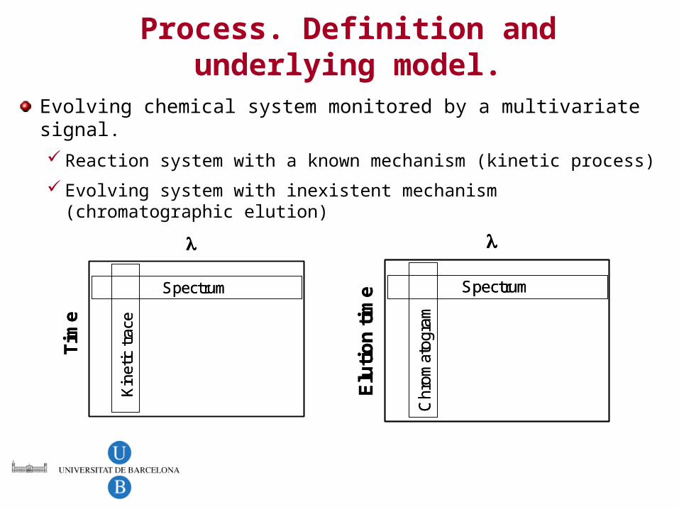
Process. Definition and underlying model.

Evolving chemical system monitored by a multivariate signal.

Reaction system with a known mechanism (kinetic process)

Evolving system with inexistent mechanism (chromatographic elution)

Tim

e

Spectrum

Kin

etic

tra

ce

Tim

e

Spectrum

Kin

etic

tra

ce

Elu

tio

nti

me

Spectrum

Chr

omat

ogra

m

Elu

tio

nti

me

Spectrum

Chr

omat

ogra

m

D DA DB

= +

DADB

D

= +

s A

cB

s B

cA

A cB

sA

c

sB

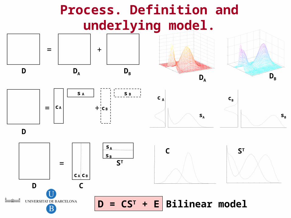
Process. Definition and underlying model.

D

=

C

ST

sB

sA

cBcA

C ST

D = CST + E Bilinear model

Known mechanism

Hard-modeling (HM)No mechanism

Soft-modeling (SM)

Process. Definition and underlying model.

=

D

Tim

e

A B C

CST

A B C

Wavelength

Ab

so

rba

nc

e

Time

Co

nc

en

tra

tio

n

Wavelength

Ab

so

rpti

vit

ies

Wavelength

Ab

so

rba

nc

e

Wavelength

Ab

so

rba

nc

e

Time

Co

nc

en

tra

tio

n

Time

Co

nc

en

tra

tio

n

Wavelength

Ab

so

rpti

vit

ies

Wavelength

Ab

so

rpti

vit

ies

WavelengthsRetention times WavelengthsWavelengthsRetention timesRetention times

Ordered evolving concentration pattern

Process soft-modeling(Multivariate Curve Resolution, MCR)

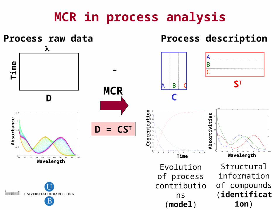
MCR in process analysis

D

Tim

e

0 10 20 30 40 50 60 70 80 90 1000

0.5

1

1.5

2

2.5

Wavelength

Ab

so

rba

nc

e

Process raw data

=

A B C

C

ST

A B C

0 1 2 3 4 5 6 7 8 9 100

0.1

0.2

0.3

0.4

0.5

0.6

0.7

0.8

0.9

1

Time

Co

nc

en

tra

tio

n0 10 20 30 40 50 60 70 80 90 100

0

0.5

1

1.5

2

2.5

3x 10

4

Wavelength

Ab

so

rtiv

itie

s

D = CST

Process description

MCR

Evolution of process

contributions(model)

Structural information of compounds

(identification)

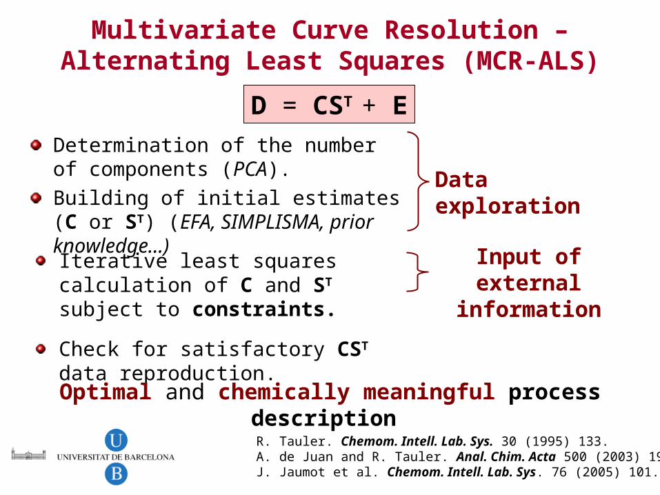
Multivariate Curve Resolution – Alternating Least Squares (MCR-ALS)

Determination of the number of components (PCA).

Building of initial estimates (C or ST) (EFA, SIMPLISMA, prior knowledge...)

Iterative least squares calculation of C and ST subject to constraints.

Check for satisfactory CST data reproduction.

Data exploration

Input of external information

Optimal and chemically meaningful process description

D = CST + E

R. Tauler. Chemom. Intell. Lab. Sys. 30 (1995) 133. A. de Juan and R. Tauler. Anal. Chim. Acta 500 (2003) 195.J. Jaumot et al. Chemom. Intell. Lab. Sys. 76 (2005) 101.

Constraints

DefinitionAny property systematically present in the profiles of the compounds in our data set.

Chemical origin Mathematical properties.

ApplicationC and S can be constrained differently.

The profiles within C and ST can be constrained differently.

Reflect the inherent order in a process

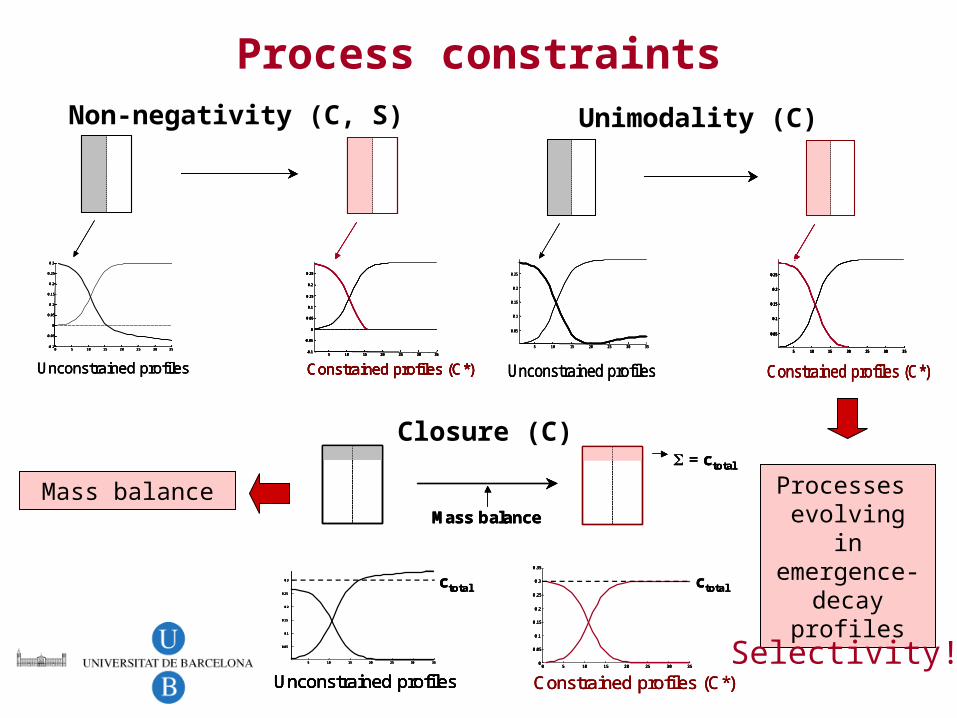
Process constraints

Unconstrained profiles

0 5 10 15 20 25 30 35-0.1

-0.05

0

0.05

0.1

0.15

0.2

0.25

0.3

Constrained profiles (C*)5 10 15 20 25 30 35

-0.1

-0.05

0

0.05

0.1

0.15

0.2

0.25

Unconstrained profiles

0 5 10 15 20 25 30 35-0.1

-0.05

0

0.05

0.1

0.15

0.2

0.25

0.3

Unconstrained profiles

0 5 10 15 20 25 30 35-0.1

-0.05

0

0.05

0.1

0.15

0.2

0.25

0.3

0 5 10 15 20 25 30 35-0.1

-0.05

0

0.05

0.1

0.15

0.2

0.25

0.3

Constrained profiles (C*)5 10 15 20 25 30 35

-0.1

-0.05

0

0.05

0.1

0.15

0.2

0.25

Constrained profiles (C*)5 10 15 20 25 30 35

-0.1

-0.05

0

0.05

0.1

0.15

0.2

0.25

Constrained profiles (C*)5 10 15 20 25 30 35

-0.1

-0.05

0

0.05

0.1

0.15

0.2

0.25

Constrained profiles (C*)5 10 15 20 25 30 35

-0.1

-0.05

0

0.05

0.1

0.15

0.2

0.25

5 10 15 20 25 30 35-0.1

-0.05

0

0.05

0.1

0.15

0.2

0.25

Non-negativity (C, S)

Unconstrained profiles

5 10 15 20 25 30 35

0.05

0.1

0.15

0.2

0.25

Constrained profiles (C*)

5 10 15 20 25 30 35

0.05

0.1

0.15

0.2

0.25

Unconstrained profiles

5 10 15 20 25 30 35

0.05

0.1

0.15

0.2

0.25

Unconstrained profiles

5 10 15 20 25 30 35

0.05

0.1

0.15

0.2

0.25

5 10 15 20 25 30 35

0.05

0.1

0.15

0.2

0.25

Constrained profiles (C*)

5 10 15 20 25 30 35

0.05

0.1

0.15

0.2

0.25

Constrained profiles (C*)

5 10 15 20 25 30 35

0.05

0.1

0.15

0.2

0.25

Constrained profiles (C*)

5 10 15 20 25 30 35

0.05

0.1

0.15

0.2

0.25

5 10 15 20 25 30 35

0.05

0.1

0.15

0.2

0.25

5 10 15 20 25 30 35

0.05

0.1

0.15

0.2

0.25

5 10 15 20 25 30 35

0.05

0.1

0.15

0.2

0.25

Unimodality (C)

Processes evolving in

emergence-decay profilesctotal

Unconstrained profiles5 10 15 20 25 30 35

0.05

0.1

0.15

0.2

0.25

0.3

Mass balance

= ctotal

ctotal

Constrained profiles (C*)0 5 10 15 20 25 30 35

0

0.05

0.1

0.15

0.2

0.25

0.3

0.35

ctotal

Unconstrained profiles5 10 15 20 25 30 35

0.05

0.1

0.15

0.2

0.25

0.3 ctotal

Unconstrained profiles5 10 15 20 25 30 35

0.05

0.1

0.15

0.2

0.25

0.3

Unconstrained profiles5 10 15 20 25 30 35

0.05

0.1

0.15

0.2

0.25

0.3

5 10 15 20 25 30 35

0.05

0.1

0.15

0.2

0.25

0.3

Mass balanceMass balance

= ctotal

ctotal

Constrained profiles (C*)0 5 10 15 20 25 30 35

0

0.05

0.1

0.15

0.2

0.25

0.3

0.35

= ctotal

ctotal

Constrained profiles (C*)0 5 10 15 20 25 30 35

0

0.05

0.1

0.15

0.2

0.25

0.3

0.35

0 5 10 15 20 25 30 350

0.05

0.1

0.15

0.2

0.25

0.3

0.35

Closure (C)

Mass balance

Selectivity!!

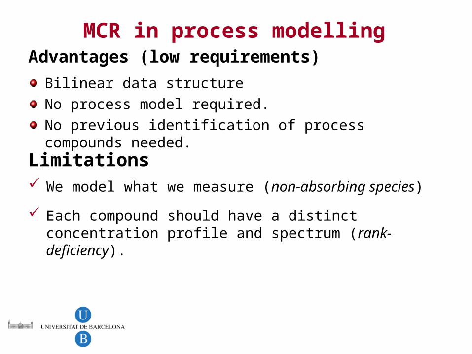
MCR in process modellingAdvantages (low requirements)

Bilinear data structure

No process model required.

No previous identification of process compounds needed.

Limitations We model what we measure (non-absorbing species)

Each compound should have a distinct concentration profile and spectrum (rank-deficiency).

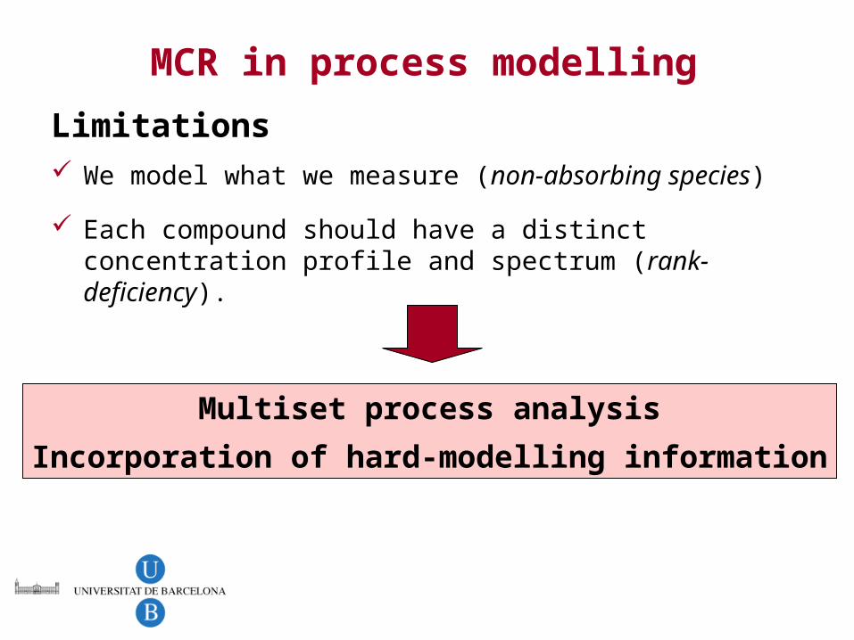
MCR in process modelling

Limitations We model what we measure (non-absorbing species)

Each compound should have a distinct concentration profile and spectrum (rank-deficiency).

Multiset process analysis

Incorporation of hard-modelling information

Advanced process modelingMultiset analysis

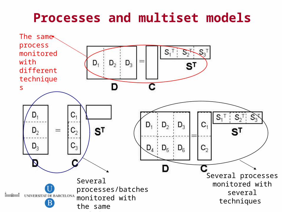
Processes and multiset modelsThe same process monitored with different techniques

Several processes/batches monitored with the same technique

Several processes monitored with several

techniques

Multiset arrangements. Advantages.

The chemometric reasons Rotational ambiguity decreases/is suppressed. Rank-deficiency problems are solved. Noise effect is minimized

The chemical reasons More information introduced in the process modelling. More robustness in the process description. Better characterization of process compounds

(multitechnique analysis). More global description of process evolution and of effect of

inducing agents. (multiexperiment analysis).

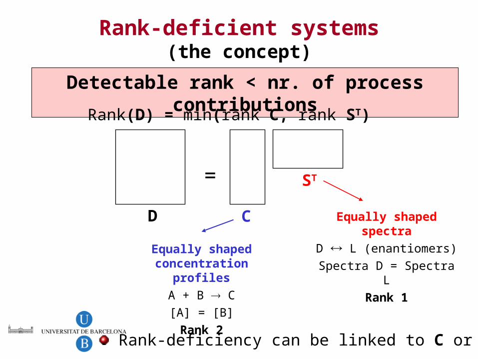
Rank-deficient systems(the concept)

Detectable rank < nr. of process contributions

=

D C

ST

Rank(D) = min(rank C, rank ST)

Equally shaped concentration profiles

A + B C

[A] = [B]

Rank 2

Equally shaped spectra

D L (enantiomers)

Spectra D = Spectra L

Rank 1

Rank-deficiency can be linked to C or to ST

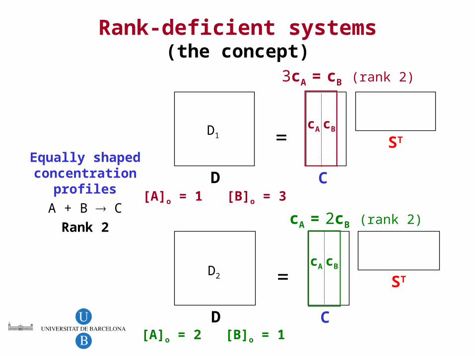
Rank-deficient systems(the concept)

Equally shaped concentration profiles

A + B C

Rank 2

=

D C

ST

cBcA

[A]o = 1 [B]o = 3

3cA = cB (rank 2)

D1

=

D C

ST

[A]o = 2 [B]o = 1

cBcA

cA = 2cB (rank 2)

D2

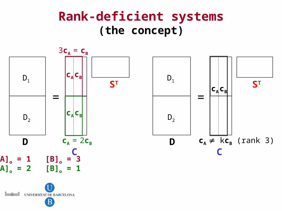
Rank-deficient systems(the concept)

[A]o = 1 [B]o = 3[A]o = 2 [B]o = 1

3cA = cB

=ST

cBcAD1

DC

cBcA

cA = 2cB

D2

=ST

D1

DC

cBcA

cA kcB (rank 3)

D2

Breaking rank-deficiency(multiset data)

=

C

SUVT

sA = ksB

sB

sA

SCDT

sA ksB

sB

sA

DUV

D

DCD

=

C

ST

sB

sA

DUV

D

DCD

sA ksB

(rank 2)

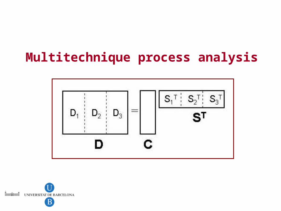
Multitechnique process analysis

Multitechnique data analysis

Only the concentration direction is shared by all experiments. Completely different techniques can be treated together

Higher spectral discrimination power among compounds.

The augmented response contains complementary information of all techniques (‘superspectrum’).

The single matrix of process profiles provides cleaner process profiles and a more robust description of the process.

Process profiles are not affected by specific noise patterns of particular techniques.

Process description should be valid for all measurements collected.

Multiset multi-way

ON

FeON

Fe

pH-induced transitions in hemoglobin

Spectroscopic monitoring between pH 1.5 and 10.5 Changes in secondary structure

UV (350-650 nm), far-UV CD (200-250 nm) Changes in tertiary structure

UV, near-UV CD (250-350 nm), fluorescence (300-450 nm)

Binding of heme group

UV, Soret CD (380-430 nm)

Evolution of protein conformations Global process: many events at different structural levels. No mechanism defined.

Muñoz, G.; de Juan, A. Anal. Chim. Acta 2007, 595, 198.

pH-induced transitions in hemoglobin(single technique resolution)

D1pH D2

pH D3pH D4

pH D5pH

UVFar-UV CD

200 210 220 230 240 250

-15

-10

-5

0

5

10

15

20

D1

300 350 400 4500

0.02

0.04

0.06

0.08

0.1

0.12

0.14

0.16

0.18

D4

350 450 550 6500

0.2

0.4

0.6

0.8

1

D5

Fluorescence

250 275 300 325 350-4

-2

0

2

4

6

8

10

D3

Near-UV CD

Wavelengths (nm)

Soret CD

380 390 400 410 420 430-10

-5

0

5

10

15

20

D2

Wavelengths (nm)Wavelengths (nm) Wavelengths (nm) Wavelengths (nm)

pH1.5 10.5

2ary structure 3ary structureHeme binding Global

pH-induced transitions in hemoglobin(single technique resolution)

Technique Chemical eventNr. of

process contributions

pH transition values

Explained variance (%)

Far-UV CD Changes 2ary structure 2 4.0 99.75

Near-UV CD Changes 3ary structure 2 4.5 93.83

Fluorescence Changes 3ary structure 3 4.2 / 8.7 99.96

Soret CD Heme binding 2 7.8 99.77

UV-visible Global process 4 2.8 / 3.9 / 8.5 99.75

Some chemical events are simpler than the global process.

Non absorbing species are not modelled.

Too similar spectral contributions may not be distinguished.

Multitechnique analysis is needed to complete the puzzle.

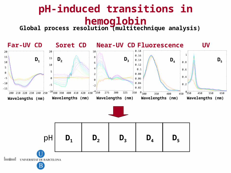
pH-induced transitions in hemoglobinGlobal process resolution (multitechnique analysis)

D1 D2 D3 D4 D5pH

UVFar-UV CD

200 210 220 230 240 250

-15

-10

-5

0

5

10

15

20

D1

300 350 400 4500

0.02

0.04

0.06

0.08

0.1

0.12

0.14

0.16

0.18

D4

350 450 550 6500

0.2

0.4

0.6

0.8

1

D5

FluorescenceNear-UV CD

250 275 300 325 350-4

-2

0

2

4

6

8

10

D3

Wavelengths (nm)

Soret CD

380 390 400 410 420 430-10

-5

0

5

10

15

20

D2

Wavelengths (nm)Wavelengths (nm) Wavelengths (nm) Wavelengths (nm)

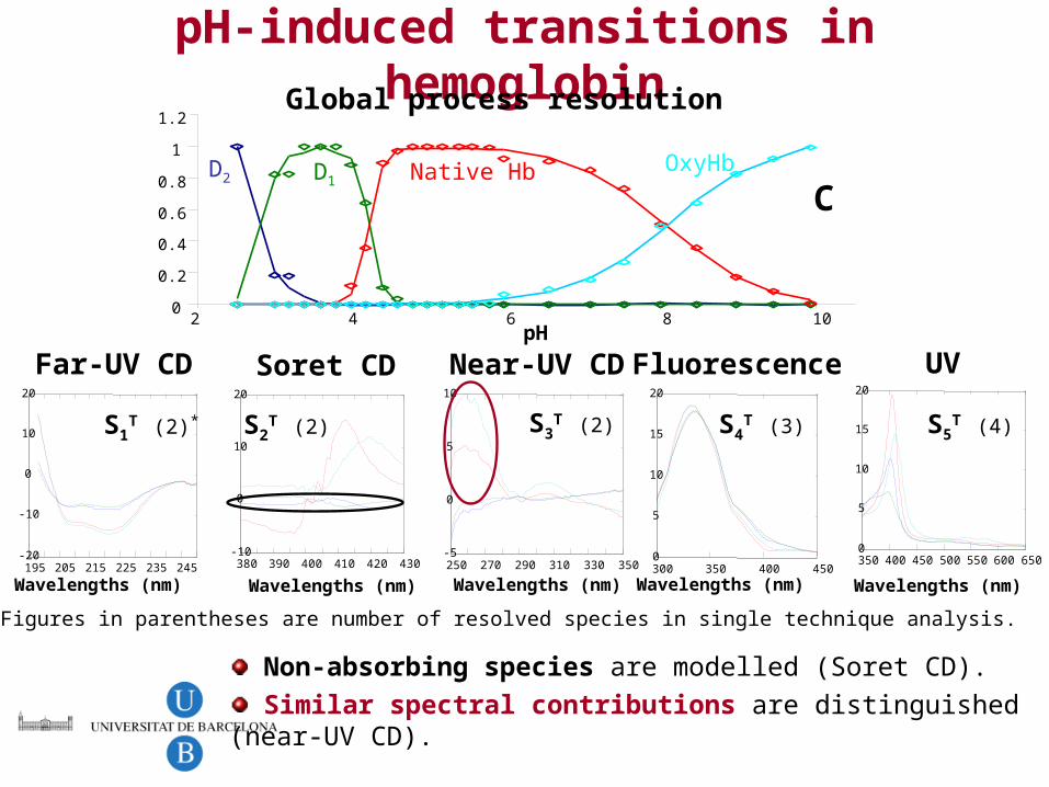
pH-induced transitions in hemoglobinGlobal process resolution

300 350 400 4500

5

10

15

20

Fluorescence

Wavelengths (nm)195 205 215 225 235 245

-20

-10

0

10

20

Far-UV CD

Wavelengths (nm)

350 400 450 500 550 600 6500

5

10

15

20

UV

Wavelengths (nm)250 270 290 310 330 350-5

0

5

10

Near-UV CD

Wavelengths (nm)380 390 400 410 420 430

-10

0

10

20

Soret CD

Wavelengths (nm)

pH0

0.2

0.4

0.6

0.8

1

1.2

2 4 6 8 10

Non-absorbing species are modelled (Soret CD).

Similar spectral contributions are distinguished (near-UV CD).

C

S1T (2)* S3

T (2)S2T (2) S4

T (3) S5T (4)

* Figures in parentheses are number of resolved species in single technique analysis.

Native HbD1OxyHbD2

Multiexperiment process analysis

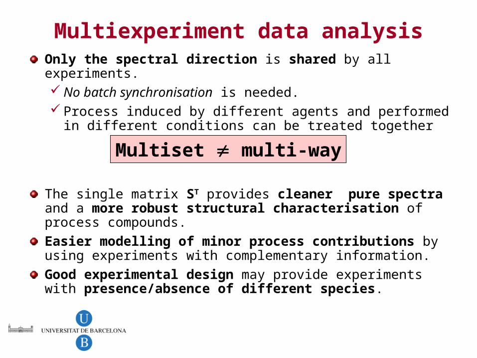
Multiexperiment data analysisOnly the spectral direction is shared by all experiments. No batch synchronisation is needed. Process induced by different agents and performed in

different conditions can be treated together

The single matrix ST provides cleaner pure spectra and a more robust structural characterisation of process compounds.

Easier modelling of minor process contributions by using experiments with complementary information.

Good experimental design may provide experiments with presence/absence of different species.

Multiset multi-way

Protein-drug interaction

Dominant at low [ligand:protein] ratio

and low [ligand].

Meso-tetrakis(p-sulf onatephenyl )porphyrin (TSPP)

Loop E-FGlu89

cavity

-lactoglobulin Meso-tetrakis(p-sulf onatephenyl )porphyrin (TSPP)

Loop E-FGlu89

cavity

Loop E-FGlu89

cavity

Loop E-FGlu89

cavity

Loop E-FGlu89

cavity

-lactoglobulin Meso-tetrakis(p-sulf onatephenyl )porphyrin (TSPP)

Loop E-FGlu89

cavity

Loop E-FGlu89

cavity

Loop E-FGlu89

cavity

Loop E-FGlu89

cavity

-lactoglobulin Meso-tetrakis(p-sulf onatephenyl )porphyrin (TSPP)

Loop E-FGlu89

cavity

Loop E-FGlu89

cavity

Loop E-FGlu89

cavity

Loop E-FGlu89

cavity

Loop E-FGlu89

cavity

Loop E-FGlu89

cavity

Loop E-FGlu89

cavity

-lactoglobulin

Protein + TSPP [Protein-TSPP]complex TSPPaggregate

Dominant at high [ligand:protein] ratio and

high [ligand].

Multiexperiment analysis of experiments enhancing low and high [protein:ligand] ratios help in the definition of all species involved.

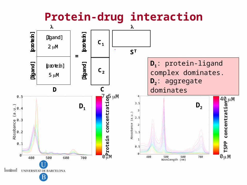
Protein-drug interaction

D1: protein-ligand complex dominates.D2: aggregate dominates

=

[ligand]

2 M

[protein]

5 M

[p

rote

in]

[lig

and

]

C

ST.

C1

C2

D

[pro

tein

][l

igan

d]

=

[ligand]

2 M

[protein]

5 M

[p

rote

in]

[lig

and

]

C

ST.

C1

C2

D

[pro

tein

][l

igan

d]

400 500 600 7000

0.1

0.2

0.3

0.4

0.5

Abso

ban

ce (

a.u

.)

0 M

7.5 M

Pro

tein

con

cen

trati

on

D1

400 500 600 7000

0.5

1

1.5

2

2.5

3

3.5

4

Wavelength (nm)

Ab

sorb

ance

(a.u

.)

0 M

40 M

TS

PP

con

cen

trati

on

D2

Protein-drug interaction

350 400 450 500 550 600 650 700 7500

0.05

0.1

0.15

0.2

0.25

0.3

0.35

Wavelength (nm)

Ab

sorb

ance

(a.u

.)

ST

0 5 10 15 20 25 30 35 400

5

10

15

20

25

TSPP concentration ( M)

Con

cent

rati

on (

a.u.

)

TSPPProtein-TSPP

TSPPaggregate

C2

TSPPProtein-TSPP

C1

0 1 2 3 4 5 6 70

2

4

6

8

10

12

Protein concentration (M)

Con

cent

rati

on (

a.u.

)

0 5 10 15 20 25 30 35 400

5

10

15

20

25

TSPP concentration ( M)TSPP concentration ( M)

Con

cent

rati

on (

a.u.

)

TSPPProtein-TSPP

TSPPaggregate

C2

TSPPProtein-TSPP

C1

0 1 2 3 4 5 6 70

2

4

6

8

10

12

Protein concentration (M)

Con

cent

rati

on (

a.u.

)

TSPPProtein-TSPP

C1

0 1 2 3 4 5 6 70

2

4

6

8

10

12

Protein concentration (M)Protein concentration (M)

Con

cent

rati

on (

a.u.

)

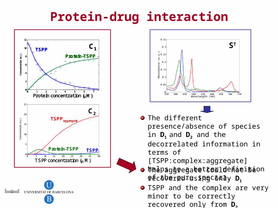
The aggregate could not be recovered using only D1

TSPP and the complex are very minor to be correctly recovered only from D2

The different presence/absence of species in D1 and D2 and the decorrelated information in terms of [TSPP:complex:aggregate] helps to a better definition of the pure spectra.

Advanced process modeling(Incorporating hard models)

Process modelling

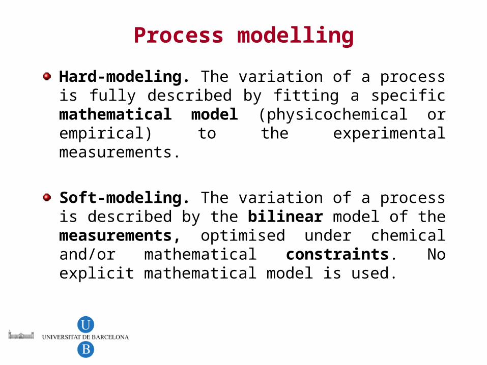
Hard-modeling. The variation of a process is fully described by fitting a specific mathematical model (physicochemical or empirical) to the experimental measurements.

Soft-modeling. The variation of a process is described by the bilinear model of the measurements, optimised under chemical and/or mathematical constraints. No explicit mathematical model is used.

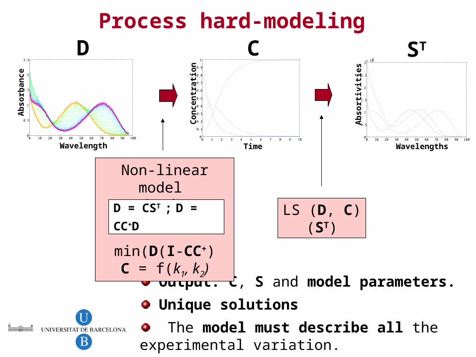
Process hard-modeling

0 10 20 30 40 50 60 70 80 90 1000

0.5

1

1.5

2

2.5

3x 104

Wavelengths

Ab

so

rtiv

itie

s

LS (D, C)(ST)

ST

Output: C, S and model parameters.

Unique solutions

The model must describe all the experimental variation.

0 10 20 30 40 50 60 70 80 90 1000

0.5

1

1.5

2

2.5

Wavelength

Ab

so

rba

nc

e

0 1 2 3 4 5 6 7 8 9 100

0.1

0.2

0.3

0.4

0.5

0.6

0.7

0.8

0.9

1

Time

Co

nc

en

tra

tio

n

D C

Non-linear model Fitting

min(D(I-CC+)C = f(k1, k2)

D = CST ; D = CC+D

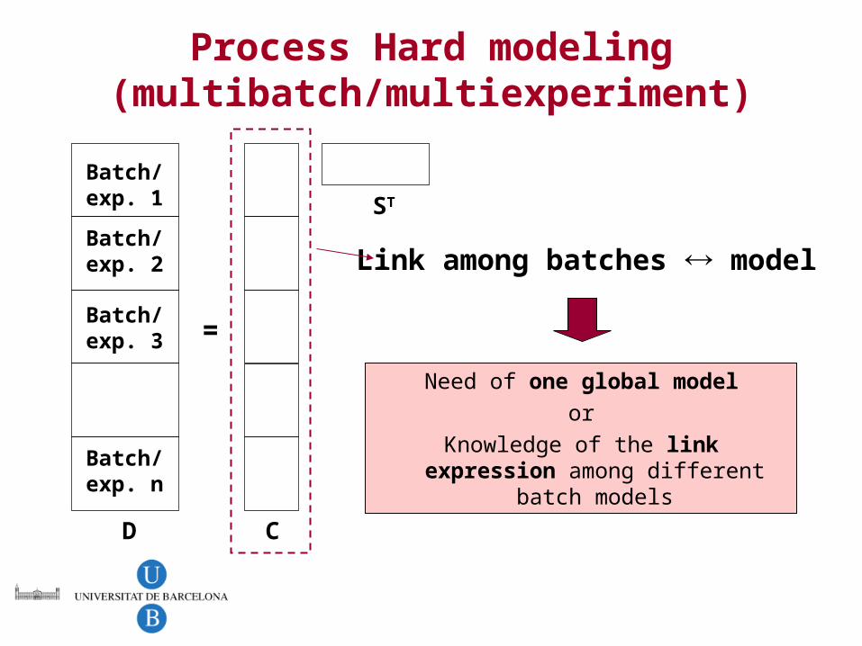
Process Hard modeling (multibatch/multiexperiment)

Need of one global model

or

Knowledge of the link expression among different batch models

Batch/exp. 1

D C

ST

=

Batch/exp. 2

Batch/exp. 3

Batch/exp. n

Link among batches model

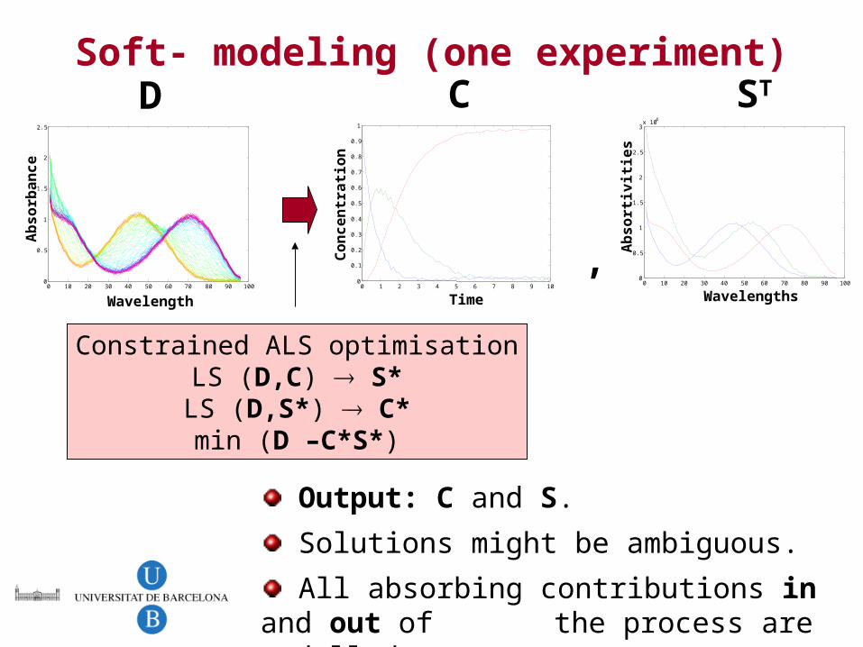
Soft- modeling (one experiment)

0 10 20 30 40 50 60 70 80 90 1000

0.5

1

1.5

2

2.5

3x 104

Wavelengths

Ab

so

rtiv

itie

s

ST

0 10 20 30 40 50 60 70 80 90 1000

0.5

1

1.5

2

2.5

Wavelength

Ab

so

rba

nc

e

D C

Constrained ALS optimisationLS (D,C) S*LS (D,S*) C*min (D –C*S*)

,

Output: C and S.

Solutions might be ambiguous.

All absorbing contributions in and out of the process are modelled.

0 1 2 3 4 5 6 7 8 9 100

0.1

0.2

0.3

0.4

0.5

0.6

0.7

0.8

0.9

1

Time

Co

nc

en

tra

tio

n

Soft-modeling (multibatch/multiexperiment)

Batch/exp. 1

D C

ST

=

Batch/exp. 2

Batch/exp. 3

Batch/exp. n

Different experiments can be analysed together

Experimental conditions, link among batches may be unknown.

Link among batches pure spectra

Incorporating hard-modeling in MCR

All or some of the concentration profiles can be constrained.

All or some of the batches can be constrained.

A B C X

C C

0 1 2 3 4 5 6 7 8 9 100

0.1

0.2

0.3

0.4

0.5

0.6

0.7

0.8

0.9

1

Time

Con

cent

ratio

n (a

.u.)

A

B

C

X

0 1 2 3 4 5 6 7 8 9 100

0.1

0.2

0.3

0.4

0.5

0.6

0.7

0.8

0.9

1

Time

Con

cent

ratio

n (a

.u.)

A B C XA

B

C

X

CSM CHM

Non-linear model fitting

min(CHM - CSM)CHM = f(k1, k2)

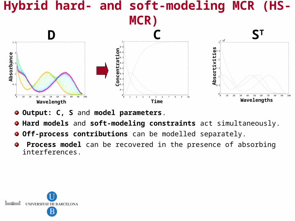
Hybrid hard- and soft-modeling MCR (HS-MCR)

Output: C, S and model parameters.

Hard models and soft-modeling constraints act simultaneously.

Off-process contributions can be modelled separately.

Process model can be recovered in the presence of absorbing interferences.

0 10 20 30 40 50 60 70 80 90 1000

0.5

1

1.5

2

2.5

3x 104

Wavelengths

Ab

so

rtiv

itie

s

ST

0 10 20 30 40 50 60 70 80 90 1000

0.5

1

1.5

2

2.5

Wavelength

Ab

so

rba

nc

e

D C

0 1 2 3 4 5 6 7 8 9 100

0.1

0.2

0.3

0.4

0.5

0.6

0.7

0.8

0.9

1

Time

Co

nc

en

tra

tio

n

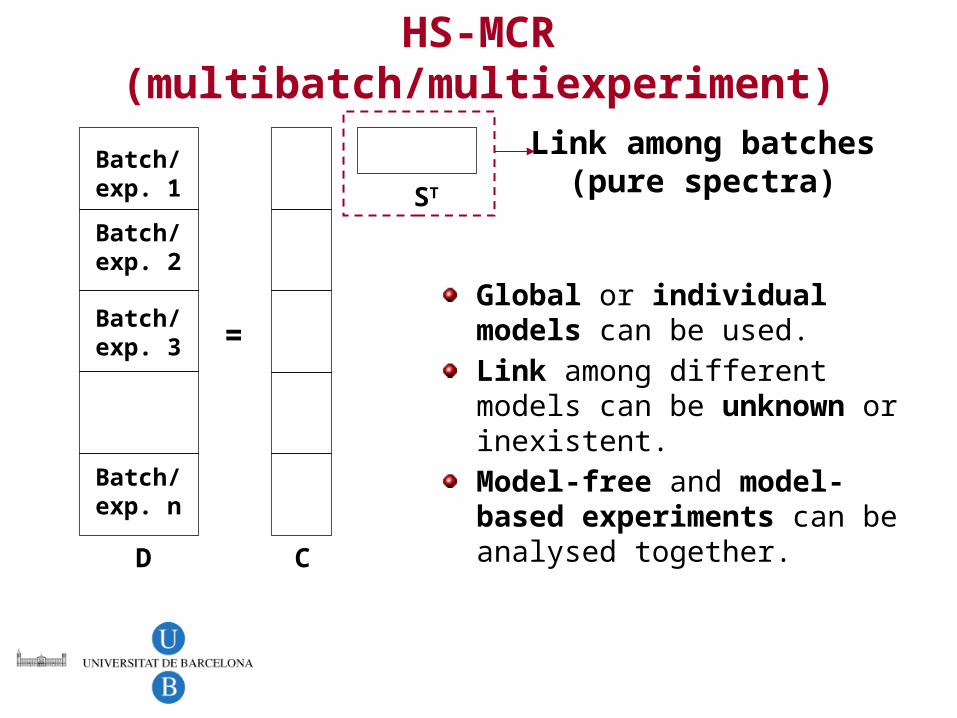
HS-MCR (multibatch/multiexperiment)

Batch/exp. 1

D C

ST

=

Batch/exp. 2

Batch/exp. 3

Batch/exp. n

Link among batches (pure spectra)

Global or individual models can be used.Link among different models can be unknown or inexistent.Model-free and model-based experiments can be analysed together.

Myoglobin denaturation

Mechanism

Steady-state process

Native (N) Intermediate (Is) Denatured (D)

Kinetic transient (It)

Kinetic process

Steady-state processUV spectra, pH range 7.0-2.0

N Is ? D

Unknown model

Kinetic processUV spectra, pH-jump stopped-flow

First-order consecutive reactions

D?IN 21 kt

k

P. Culberg, P.J. Gemperline, A. de Juan. (submitted)

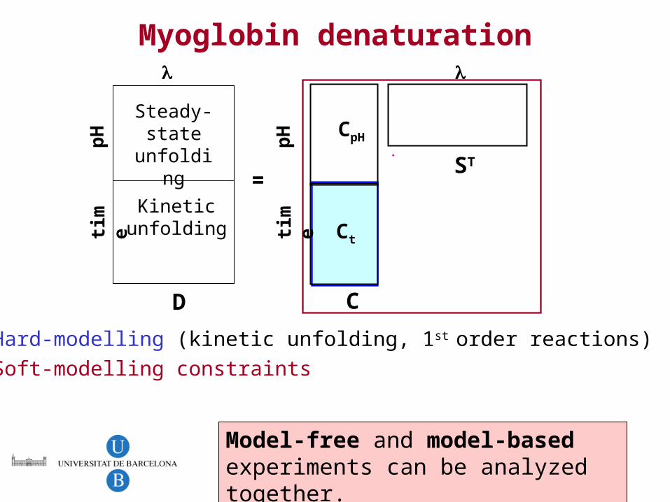
Hard-modelling (kinetic unfolding, 1st order reactions)

Soft-modelling constraints

Myoglobin denaturation

=

Steady-state

unfolding

Kinetic unfolding

p

Hti

me

C

ST

.CpH

Ct

Dp

Hti

me

Model-free and model-based experiments can be analyzed together.

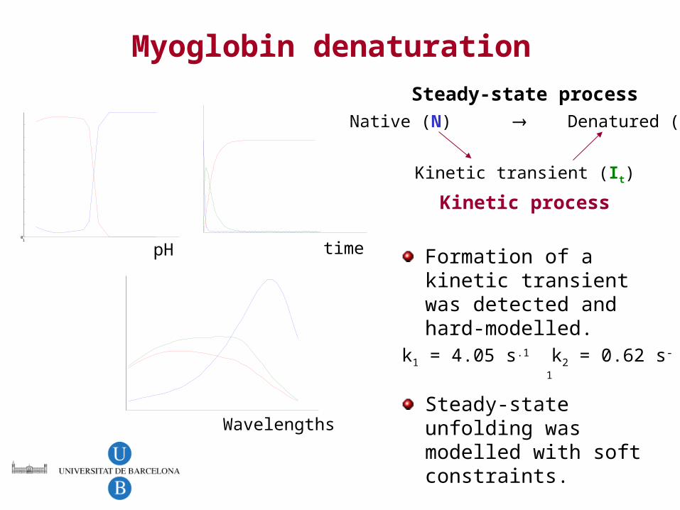
Myoglobin denaturation

Formation of a kinetic transient was detected and hard-modelled.k1 = 4.05 s.1 k2 = 0.62 s-1

Steady-state unfolding was modelled with soft constraints.

Steady-state process

Native (N) Denatured (D)

Kinetic transient (It)

Kinetic process

10

pH time

Wavelengths

BDE-209 (flame retardant)

Photodegradation of decabromodiphenil ether

OBr

Br

Br

Br

Br

Br

BrBr

BrBr

UV kinetic monitoring in several THF/ water mixtures(10% water, 20% water, 30% water, 40% water)

Three replicates per solvent composition.

Wavelength (nm)

S. Mas, A. de Juan, S. Lacorte, R. Tauler (submitted)

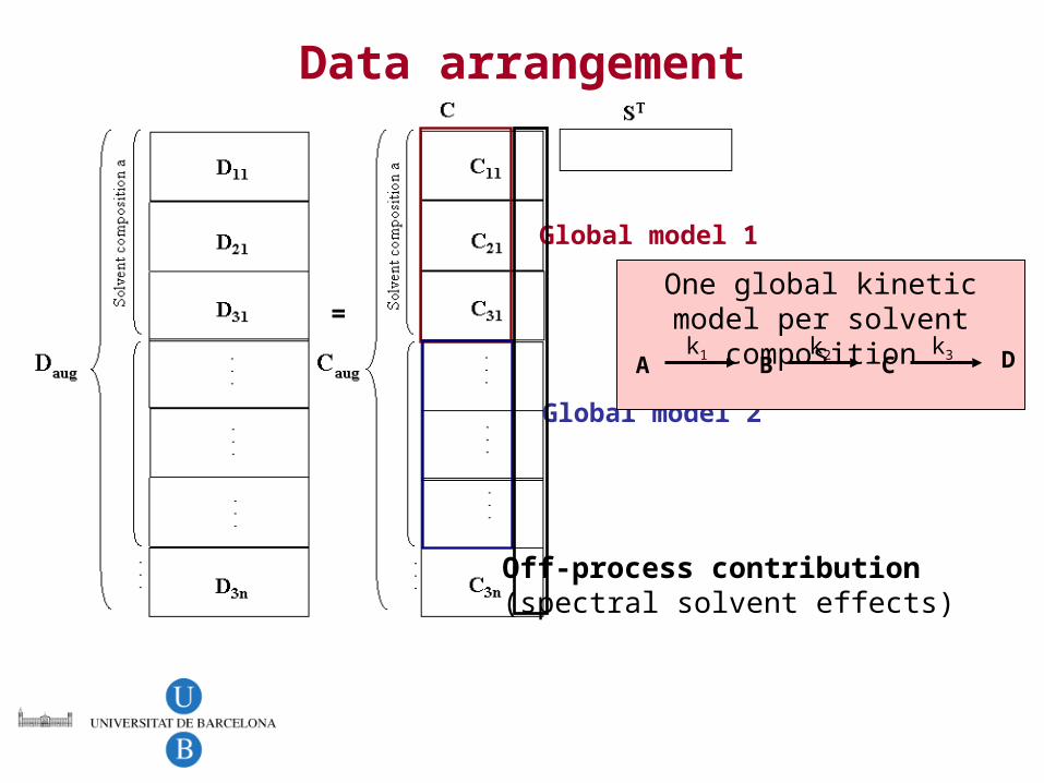
Data arrangement

Global model 1

Global model 2

One global kinetic model per solvent composition

k3 C

k2 B

k1 A D

Off-process contribution(spectral solvent effects)

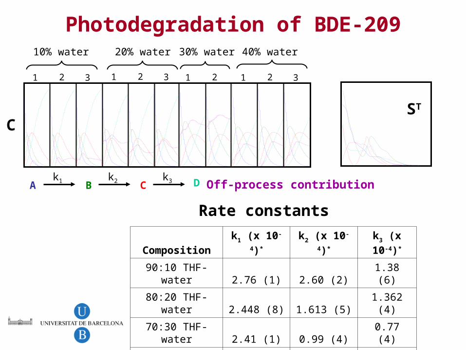
Photodegradation of BDE-20940% water

C

10% water 20% water 30% water

1 2 3 1 2 3 1 2 1 2 3

ST

Composition k1 (x 10-4)* k2 (x 10-4)* k3 (x 10-4)*

90:10 THF-water 2.76 (1) 2.60 (2) 1.38 (6)

80:20 THF-water 2.448 (8) 1.613 (5) 1.362 (4)

70:30 THF-water 2.41 (1) 0.99 (4) 0.77 (4)

60:40 THF-water 1.933 (6) 1.092 (3) 0.68 (2)

k3 C

k2 B

k1 A D Off-process contribution

Rate constants

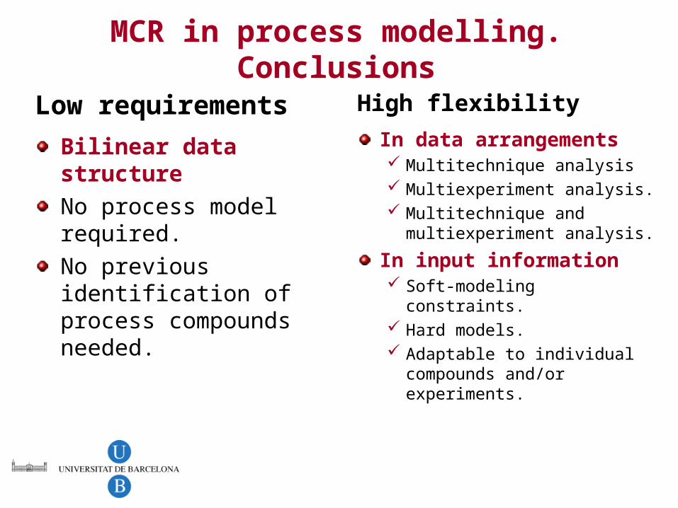
MCR in process modelling. Conclusions

Low requirements

Bilinear data structure

No process model required.

No previous identification of process compounds needed.

High flexibility

In data arrangements Multitechnique analysis Multiexperiment analysis. Multitechnique and

multiexperiment analysis.

In input information Soft-modeling constraints. Hard models. Adaptable to individual

compounds and/or experiments.

Acknowledgements

Glòria Muñoz (pH-dependent hemoglobin example)

Susana Navea (Protein-drug interaction).

Sílvia Mas (UB and IIQAB-CSIC) (BDE-209 example)

Pat Culberg, East Carolina University (myoglobin example).

Lionel Blanchet, UB and Université des Sciences et Technologies de Lille (photochemical example)

Financial support by Spanish Government

Group Web page: www.ub.es/gesq/mcr/mcr.htm

Process. Definition and underlying model.

Evolving chemical system monitored by a multivariate signal.

Reaction system with a known mechanism (kinetic process)

Evolving system with inexistent mechanism (chromatographic elution)

Pro

cess

var

iab

leMeasurement channel

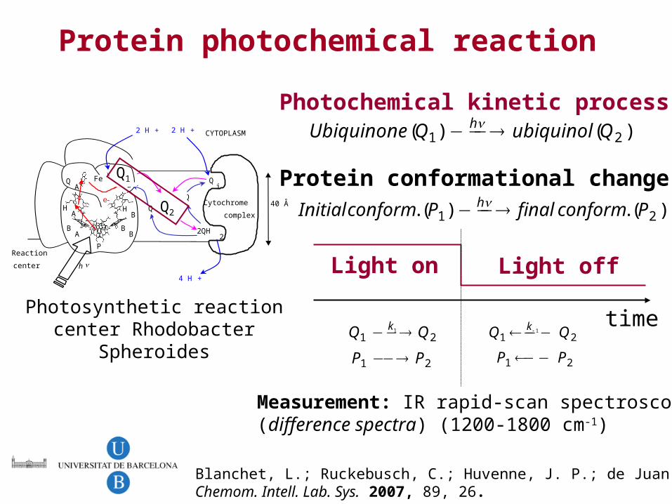
Protein photochemical reaction

Photochemical kinetic process

Protein conformational change

)()( 21 QubiquinolQUbiquinone h

)(.)(. 21 PconformfinalPconformInitial h

Light on Light off

time21

1 QQ k 211 QQ k

21 PP 21 PP

Measurement: IR rapid-scan spectroscopy(difference spectra) (1200-1800 cm-1)

Fe

P

BA

HA

QA

QB

HB

BB

Qi

2QH2

QH2

Q

Q40 ÅCytochrome

complex

Reaction

center

CYTOPLASM2 H + 2 H +

4 H +

h

e-

Q1

Q2

Photosynthetic reaction center Rhodobacter Spheroides

Blanchet, L.; Ruckebusch, C.; Huvenne, J. P.; de Juan, A. Chemom. Intell. Lab. Sys. 2007, 89, 26.

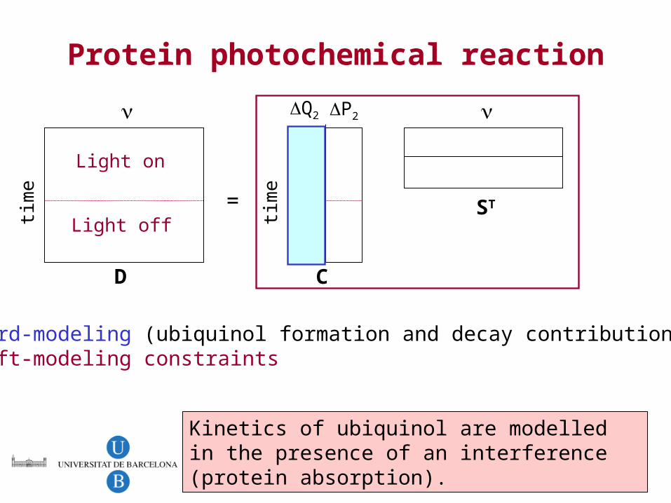
Protein photochemical reactiontim

e

Light on

Light off

Kinetics of ubiquinol are modelled in the presence of an interference (protein absorption).

time

Q2 P2

C

ST

Hard-modeling (ubiquinol formation and decay contribution)Soft-modeling constraints

=

D

Protein photochemical reaction

Kinetics of ubiquinol formation and decay are modelled (hard-modeling constraint).

k1 = 7 10-4 s-1

k-1 = 10-4 s-1

Photoinduced protein conformational change (model-free) is modelled.

-2

-1

0

1

2

OffOn

Time (s)

Wavenumber (cm-1)

12001800

60

Amide IIAmide I

-Q1

+Q2

Rotational ambiguity and noise minimization

Single setof process profilesfor all techniques

C,ST possible combinations with optimal fit are less(rotational ambiguity

decreases)

Noise is technique- and data set-dependent.

C encloses common information for all techniques (noise effect is minimized)

Breaking rank-deficiency(multiset data)

=

D C

SCDT

sA ksB

(rank 2)sB

sA

DCD

=

D C

SUVT

sA = ksB

(rank 1)sB

sA

DUV

Equally shaped spectra

D L (enantiomers)

Spectra D = Spectra L

Rank 1

D = CST

D = CT inv(T)ST