advanced power systems analysis tools - digital library/67531/metadc717935/m2/1/high... · subtask...

SUBTASK 3.6 – ADVANCED POWER SYSTEMSANALYSIS TOOLS

Final Report

(for the Reporting Period April 1, 2000 through August 31, 2001)

Prepared for:

AAD Document ControlU.S. Department of EnergyNational Energy Technology LaboratoryPO Box 10940, MS 921-143Pittsburgh, PA 15236-0940

Cooperative Agreement No. DE-FC26-98FT40320; UND Fund 4373Performance Monitor: Philip Goldberg

Prepared by:

Robert R. JensenSteven A. Benson

Jason D. Laumb

Energy & Environmental Research CenterUniversity of North Dakota

PO Box 9018Grand Forks, ND 58202-9018

2001-EERC-08-05 August 2001

DOE DISCLAIMER

This report was prepared as an account of work sponsored by an agency of the United StatesGovernment. Neither the United States Government, nor any agency thereof, nor any of theiremployees makes any warranty, express or implied, or assumes any legal liability or responsibilityfor the accuracy, completeness, or usefulness of any information, apparatus, product, or processdisclosed or represents that its use would not infringe privately owned rights. Reference herein toany specific commercial product, process, or service by trade name, trademark, manufacturer, orotherwise does not necessarily constitute or imply its endorsement, recommendation, or favoring bythe United States Government or any agency thereof. The views and opinions of authors expressedherein do not necessarily state or reflect those of the United States Government or any agencythereof.

This report is available to the public from the National Technical Information Service, U.S.Department of Commerce, 5285 Port Royal Road, Springfield, VA 22161; phone orders acceptedat (703) 487-4650.

ACKNOWLEDGMENT

This report was prepared with the support of the U.S. Department of Energy (DOE) NationalEnergy Technology Laboratory Cooperative Agreement No. DE-FC26-98FT40320. However, anyopinions, findings, conclusions, or recommendations expressed herein are those of the authors(s) anddo not necessarily reflect the views of DOE.

EERC DISCLAIMER

LEGAL NOTICE This research report was prepared by the Energy & Environmental ResearchCenter (EERC), an agency of the University of North Dakota, as an account of work sponsored byDOE. Because of the research nature of the work performed, neither the EERC nor any of itsemployees makes any warranty, express or implied, or assumes any legal liability or responsibilityfor the accuracy, completeness, or usefulness of any information, apparatus, product, or processdisclosed, or represents that its use would not infringe privately owned rights. Reference herein toany specific commercial product, process, or service by trade name, trademark, manufacturer, orotherwise does not necessarily constitute or imply its endorsement or recommendation by the EERC.

i

TABLE OF CONTENTS

LIST OF FIGURES . . . . . . . . . . . . . . . . . . . . . . . . . . . . . . . . . . . . . . . . . . . . . . . . . . . . . . . . . . . iii

LIST OF TABLES . . . . . . . . . . . . . . . . . . . . . . . . . . . . . . . . . . . . . . . . . . . . . . . . . . . . . . . . . . . . v

EXECUTIVE SUMMARY . . . . . . . . . . . . . . . . . . . . . . . . . . . . . . . . . . . . . . . . . . . . . . . . . . . . vi

INTRODUCTION . . . . . . . . . . . . . . . . . . . . . . . . . . . . . . . . . . . . . . . . . . . . . . . . . . . . . . . . . . . . 1

PROJECT GOALS AND OBJECTIVES . . . . . . . . . . . . . . . . . . . . . . . . . . . . . . . . . . . . . . . . . . 1

STATEMENT OF WORK FOR ACTIVITY 1 – MODEL DEMONSTRATIONS . . . . . . . . . . 2Activity 1 – Goals and Objectives . . . . . . . . . . . . . . . . . . . . . . . . . . . . . . . . . . . . . . . . . . . 2Activity 1 – Methods . . . . . . . . . . . . . . . . . . . . . . . . . . . . . . . . . . . . . . . . . . . . . . . . . . . . . 2

Input File for Ash Transformation Model . . . . . . . . . . . . . . . . . . . . . . . . . . . . . . . . 4CCSEM Mineral Analysis Results . . . . . . . . . . . . . . . . . . . . . . . . . . . . . . . . . . . . . . 6Ash Coal Chemical Analysis . . . . . . . . . . . . . . . . . . . . . . . . . . . . . . . . . . . . . . . . . . 6Trace Element Bulk Analysis . . . . . . . . . . . . . . . . . . . . . . . . . . . . . . . . . . . . . . . . . . 7Coal Proximate and Ultimate Analysis Results . . . . . . . . . . . . . . . . . . . . . . . . . . . . 7Trace Element Distribution Analysis . . . . . . . . . . . . . . . . . . . . . . . . . . . . . . . . . . . . 7

Output File Format for Ash Transformation Model . . . . . . . . . . . . . . . . . . . . . . . . . . . . . . 7Activity 1 – Results . . . . . . . . . . . . . . . . . . . . . . . . . . . . . . . . . . . . . . . . . . . . . . . . . . . . . . 8

STATEMENT OF WORK FOR ACTIVITY 2 – INTERACTIVE SPREADSHEETMODEL . . . . . . . . . . . . . . . . . . . . . . . . . . . . . . . . . . . . . . . . . . . . . . . . . . . . . . . . . . . . . . . . . . . . 10

Activity 2 – Goals and Objectives . . . . . . . . . . . . . . . . . . . . . . . . . . . . . . . . . . . . . . . . . . . 10Activity 2 – Methods and Results . . . . . . . . . . . . . . . . . . . . . . . . . . . . . . . . . . . . . . . . . . . 10

STATEMENT OF WORK FOR ACTIVITY 3 – ADVANCED FUELCHARACTERIZATION . . . . . . . . . . . . . . . . . . . . . . . . . . . . . . . . . . . . . . . . . . . . . . . . . . . . . . . 16

Activity 3 – Goals and Objectives . . . . . . . . . . . . . . . . . . . . . . . . . . . . . . . . . . . . . . . . . . . 16Activity 3 – Methods and Results . . . . . . . . . . . . . . . . . . . . . . . . . . . . . . . . . . . . . . . . . . . 17

NMARL Analytical Accomplishments . . . . . . . . . . . . . . . . . . . . . . . . . . . . . . . . . . . 17Improvements to SEMPC . . . . . . . . . . . . . . . . . . . . . . . . . . . . . . . . . . . . . . . . . . . . 17Modifications to CCSEM . . . . . . . . . . . . . . . . . . . . . . . . . . . . . . . . . . . . . . . . . . . . . 19

STATEMENT OF WORK FOR ACTIVITY 4 – SLAG FLOW BEHAVIOR . . . . . . . . . . . . . . 20Activity 4 – Goals and Objectives . . . . . . . . . . . . . . . . . . . . . . . . . . . . . . . . . . . . . . . . . . . 20Activity 4 – Methods . . . . . . . . . . . . . . . . . . . . . . . . . . . . . . . . . . . . . . . . . . . . . . . . . . . . . 21

Viscosity Measurement Protocol . . . . . . . . . . . . . . . . . . . . . . . . . . . . . . . . . . . . . . . 21Sample Preparation . . . . . . . . . . . . . . . . . . . . . . . . . . . . . . . . . . . . . . . . . . . . . . . . . 21

Continued . . .

ii

TABLE OF CONTENTS (continued)

Oxidizing and Reducing Atmospheres . . . . . . . . . . . . . . . . . . . . . . . . . . . . . . . . . . . 22Crucible and Bob Materials . . . . . . . . . . . . . . . . . . . . . . . . . . . . . . . . . . . . . . . . . . . 22HS–XRD Measurements . . . . . . . . . . . . . . . . . . . . . . . . . . . . . . . . . . . . . . . . . . . . . 23Equilibrium Thermodynamic Calculations . . . . . . . . . . . . . . . . . . . . . . . . . . . . . . . . 23Calculation of Slag Viscosity . . . . . . . . . . . . . . . . . . . . . . . . . . . . . . . . . . . . . . . . . . 24

Activity 4 – Results . . . . . . . . . . . . . . . . . . . . . . . . . . . . . . . . . . . . . . . . . . . . . . . . . . . . . . 24Literature Survey . . . . . . . . . . . . . . . . . . . . . . . . . . . . . . . . . . . . . . . . . . . . . . . . . . . 24Temperature of Critical Viscosity . . . . . . . . . . . . . . . . . . . . . . . . . . . . . . . . . . . . . . . 24Viscosity Models . . . . . . . . . . . . . . . . . . . . . . . . . . . . . . . . . . . . . . . . . . . . . . . . . . . 24Slagging Indices . . . . . . . . . . . . . . . . . . . . . . . . . . . . . . . . . . . . . . . . . . . . . . . . . . . . 25Mineralogical Investigations . . . . . . . . . . . . . . . . . . . . . . . . . . . . . . . . . . . . . . . . . . . 27Slag Viscosity Measurements . . . . . . . . . . . . . . . . . . . . . . . . . . . . . . . . . . . . . . . . . . 28

Suite A Samples . . . . . . . . . . . . . . . . . . . . . . . . . . . . . . . . . . . . . . . . . . . . . . . . . . . . . . . . . 29Comparison of Experimental Viscosities, Models, and Slag Indices . . . . . . . . . . . . 29Comparison of Experimental and Calculated Viscosities . . . . . . . . . . . . . . . . . . . . 32Comparison of Experimental Viscosities with Ash Fusibility Measurements . . . . . 38Comparison of Experimental Viscosities with Slagging Indices . . . . . . . . . . . . . . . 38

Suite B Samples . . . . . . . . . . . . . . . . . . . . . . . . . . . . . . . . . . . . . . . . . . . . . . . . . . . . . . . . . 38Comparison of Experimental and Calculated Viscosities . . . . . . . . . . . . . . . . . . . . 38Comparison of HT XRD Results with FACT Calculations . . . . . . . . . . . . . . . . . . . 40Model Development . . . . . . . . . . . . . . . . . . . . . . . . . . . . . . . . . . . . . . . . . . . . . . . . . 48

CONCLUSIONS . . . . . . . . . . . . . . . . . . . . . . . . . . . . . . . . . . . . . . . . . . . . . . . . . . . . . . . . . . . . . 48

REFERENCES . . . . . . . . . . . . . . . . . . . . . . . . . . . . . . . . . . . . . . . . . . . . . . . . . . . . . . . . . . . . . . 51

EXAMPLE OF OUTPUT FOR ASH TRANSFORMATION MODEL . . . . . . . . . . . Appendix A

EXAMPLE OF THE TRACE ELEMENT OUTPUT FILE . . . . . . . . . . . . . . . . . . . . Appendix B

PAPER WITH ADDITIONAL TESTING RESULTS . . . . . . . . . . . . . . . . . . . . . . . . Appendix C

iii

LIST OF FIGURES

1 Flow diagram of the Ash Transformation code . . . . . . . . . . . . . . . . . . . . . . . . . . . . . . . . . . 5

2 Layout of the files from CCSEM analysis . . . . . . . . . . . . . . . . . . . . . . . . . . . . . . . . . . . . . . 6

3 PSD in Illinois No. 6 coal . . . . . . . . . . . . . . . . . . . . . . . . . . . . . . . . . . . . . . . . . . . . . . . . . . . 9

4 Distribution of trace elements in particles less than 10 µm . . . . . . . . . . . . . . . . . . . . . . . . 10

5 Example of a supercritical steam calculation . . . . . . . . . . . . . . . . . . . . . . . . . . . . . . . . . . . 11

6 Example of material balance calculation . . . . . . . . . . . . . . . . . . . . . . . . . . . . . . . . . . . . . . 12

7 Adiabatic flame temperature calculation . . . . . . . . . . . . . . . . . . . . . . . . . . . . . . . . . . . . . . 13

8 Cost estimate calculation . . . . . . . . . . . . . . . . . . . . . . . . . . . . . . . . . . . . . . . . . . . . . . . . . . 14

9 Equation format used for regression analysis of enthalpy data . . . . . . . . . . . . . . . . . . . . . 15

10 Grey scales used to determine phases . . . . . . . . . . . . . . . . . . . . . . . . . . . . . . . . . . . . . . . . . 18

11 Frequency distribution for grey-scale images . . . . . . . . . . . . . . . . . . . . . . . . . . . . . . . . . . . 19

12 Haake Viscometer 7 VT550 system equipped with a rotating-bob viscometer . . . . . . . . . 22

13 Change in slag chemistry as it affects viscosity . . . . . . . . . . . . . . . . . . . . . . . . . . . . . . . . . 31

14 Slag sample showing viscosity measurements in a reducing gas atmosphere withoutwater vapor after reheating in the viscometer . . . . . . . . . . . . . . . . . . . . . . . . . . . . . . . . . . 32

15 Predicted versus measured viscosity . . . . . . . . . . . . . . . . . . . . . . . . . . . . . . . . . . . . . . . . . 40

16 Calculated viscosity comparisons for the lignite coal . . . . . . . . . . . . . . . . . . . . . . . . . . . . 41

17 Viscosity calculations comparisons for the subbituminous coal . . . . . . . . . . . . . . . . . . . . 41

18 Experimental viscosity curve for the lignite slag plotted with the crystalline mineralphases identified as the slag was cooled . . . . . . . . . . . . . . . . . . . . . . . . . . . . . . . . . . . . . . . 46

19 Experimental viscosity curve for the subbituminous slag plotted with the crystallinemineral phases identified as the slag was cooled . . . . . . . . . . . . . . . . . . . . . . . . . . . . . . . . 46

Continued . . .

iv

LIST OF FIGURES (continued)

20 Solid species predicted by FACT as a function of temperature for the lignite slag . . . . . . 47

21 Solid species predicted by FACT as a function of temperature for the subbituminousslag . . . . . . . . . . . . . . . . . . . . . . . . . . . . . . . . . . . . . . . . . . . . . . . . . . . . . . . . . . . . . . . . . . . 47

v

LIST OF TABLES

1 Source Code Files to the Ash Transformation Code Program . . . . . . . . . . . . . . . . . . . . . . . 3

2 Ash Transformation Coal and Trace Element Analysis Input Parameters . . . . . . . . . . . . . . 6

3 Chemical Components Used in Regression Analysis of Enthalpy Data . . . . . . . . . . . . . . 15

4 Comparison of Values of the SEM Method and XRF Method . . . . . . . . . . . . . . . . . . . . . 20

5 Comparison of Ash and Slag Composition . . . . . . . . . . . . . . . . . . . . . . . . . . . . . . . . . . . . 31

6 Comparison of Calculated Indices with Experimental Viscosities . . . . . . . . . . . . . . . . . . 33

7 Regression Analysis of Models and Predictive Indices . . . . . . . . . . . . . . . . . . . . . . . . . . . 35

8 Summary of Suite B Experimental and Calculated T250 and T80 Values . . . . . . . . . . . . . . 39

9 HT–XRD Results for Lignite Slag . . . . . . . . . . . . . . . . . . . . . . . . . . . . . . . . . . . . . . . . . . . 43

10A HT–XRD Results for Subbituminous Slag . . . . . . . . . . . . . . . . . . . . . . . . . . . . . . . . . . . . 44

10B HT–XRD Results for Subbituminous Slag . . . . . . . . . . . . . . . . . . . . . . . . . . . . . . . . . . . . 45

vi

SUBTASK 3.6 – ADVANCED POWER SYSTEMS ANALYSIS TOOLS

EXECUTIVE SUMMARY

The use of Energy & Environmental Research Center (EERC) modeling tools and improvedanalytical methods has provided key information in optimizing advanced power system design andoperating conditions for efficiency, producing minimal air pollutant emissions and utilizing a widerange of fossil fuel properties. This project was divided into four tasks: the demonstration of the ashtransformation model, upgrading spreadsheet tools, enhancements to analytical capabilities using thescanning electron microscopy (SEM), and improvements to the slag viscosity model. The ashtransformation model, Atran, was used to predict the size and composition of ash particles, whichhas a major impact on the fate of the combustion system. To optimize Atran key factors such asmineral fragmentation and coalescence, the heterogeneous and homogeneous interaction of theorganically associated elements must be considered as they are applied to the operating conditions.The resulting model’s ash composition compares favorably to measured results. Enhancements toexisting EERC spreadsheet application included upgrading interactive spreadsheets to calculate thethermodynamic properties for fuels, reactants, products, and steam with Newton Raphson algorithmsto perform calculations on mass, energy, and elemental balances, isentropic expansion of steam, andgasifier equilibrium conditions. Derivative calculations can be performed to estimate fuel heatingvalues, adiabatic flame temperatures, emission factors, comparative fuel costs, and per-unit carbontaxes from fuel analyses. Using state-of-the-art computer-controlled scanning electron microscopesand associated microanalysis systems, a method to determine viscosity using the incorporation ofgrey-scale binning acquired by the SEM image was developed. The image analysis capabilities ofa backscattered electron image can be subdivided into various grey-scale ranges that can be analyzedseparately. Since the grey scale’s intensity is dependent on the chemistry of the particle, it is possibleto map chemically similar areas which can also be related to the viscosity of that compound attemperature. A second method was also developed to determine the elements associated with theorganic matrix of the coals, which is currently determined by chemical fractionation. Mineralcompositions and mineral densities can be determined for both included and excluded minerals, aswell as the fraction of the ash that will be represented by that mineral on a frame-by-frame basis. Theslag viscosity model was improved to provide improved predictions of slag viscosity and temperatureof critical viscosity for representative Powder River Basin subbituminous and lignite coals.

1

SUBTASK 3.6 – ADVANCED POWER SYSTEMS ANALYSIS TOOLS

INTRODUCTION

The Energy & Environmental Research Center (EERC) has conducted numerous projects andprograms to develop analytical and modeling tools for characterizing fuels and fuel ash by-productsand for predicting fuel quality impact on conventional and advanced power system performance.These tools and analytical methods will provide key information that will aid in optimizing systemdesign and operation conditions for efficiency with minimal air pollutant emissions, while utilizinga wide range of fossil fuel properties. The system will be fuel-flexible, allowing for firing of a singleor a combination of fuels consisting of coal, natural gas, petroleum coke, and biomass.

The EERC has developed advanced analytical methods to measure key chemical and physicalproperties of materials that have an impact on power system performance. The series of analyticaltools includes computer-controlled scanning electron microscopy (CCSEM) with particle-by-particlecapabilities, chemical fractionation, scanning electron microscopy point count (SEMPC),wavelength-dispersive spectroscopy, trace element analysis, and strength-measuring techniques.Modeling tools have also been developed for predicting the formation of ash, deposition onrefractory and heat-transfer surfaces, slag flow behavior, and plugging of hot-gas filters. Theproperties of slags are of importance in the performance of conventional and advanced powersystems, with the temperature dependence of slag viscosity affecting slag flow and ash removabilityand producing undesirable deposition and corrosion issues. An improved method of predictingviscosity and the temperature of critical viscosity is needed to adequately predict basic ash behavior,which is crucial in developing more sophisticated boiler performance models.

PROJECT GOALS AND OBJECTIVES

The goal of this project was to utilize EERC modeling tools and analytical methods to providekey information to aid in optimizing advanced power system design and operation conditions forefficiency, with minimal air pollutant emissions, while utilizing a wide range of fossil fuelproperties. The specific tasks included:

• Demonstrate the utility of existing models at the EERC.

• Make improvements to models that have shortcomings that can be corrected efficiently,including prediction of slag viscosity.

• Enhance the application of existing spreadsheet programs developed at the EERC bygenerating user-friendly revisions and documentation that allow them to be used moreconveniently by researchers both at the EERC and outside the center.

• Enhance analytical capabilities to determine the inorganic components in fuels.

2

STATEMENT OF WORK FOR ACTIVITY 1 – MODEL DEMONSTRATIONS

Activity 1 – Goals and Objectives

The primary models, including FACT™ (commercially available) as well as ATRAN,TraceTran, and Fuel Quality Advisor (developed by the EERC), and viscosity models were comparedto actual experimental results from bench-, pilot-, and demonstration-scale advanced power systemsin order to investigate any inconsistencies. This was conducted for both gasification and combustionsystems. The EERC has significant data available on the performance of a high-temperatureadvanced furnace system for a wide range of coal types and the transport reactor development unit(TRDU) for a range of fuels. In addition, operating condition information on the fate of major,minor, and trace elements in the system was analyzed.

Activity 1 – Methods

The Ash Transformation module is an integral part of ATRAN, TraceTran, and Fuel QualityAdvisor. The module predicts the particle-size distribution along with the major and minor elements.TraceTran is specialized to predict the trace elements in addition to the major and minor elementsfor a gasification system.

The source code to the Ash transformation code consist of 23 C++ files (.CPP) and 24 headerfiles (.H) which are listed in Table 1. The CPP files contain the algorithms and actual code, whilethe header files contain definitions of the format and content of functions, constants, and variablesused in the respective CPP files.

The standard analyses methods stop the automatic analyses either when 1200 particles havebeen analyzed (#) or when 100 frames (F#) have been analyzed (each area the SEM can scan withouthaving to move the sample) at each magnification.

This means that the maximum particles entering the program would be data on 3600 particles.However, at the lower magnification analyses, the limit of 100 frames is typically reached before1200 particles have been found in these size ranges.

The ash transformation algorithm flow diagram is illustrated in Figure 1. The entrained ashPSCD (particle size and composition distribution) is predicted from the distribution of the inorganicsin the coal using advanced coal characterization techniques. CCSEM (1), x-ray fluorescence (XRF),and ultimate analysis are used to characterize the major elements in the coal. The CCSEM analysisis also combined with a locked/liberated particle analysis (to determine if the individual mineralgrains are located within a coal matrix or are free mineral grains) and ZAF data reduction of thecompositions (2, 3). The ZAF data reduction produces compositions free of the effects of atomicnumber (Z), x-ray absorption (A), and XRF (F). A mass balance is compiled on the coal bycomparing the CCSEM and XRF data. The resultant balance provides the compositions of theminerals with their associations to the coal, organically associated constituents, and submicronparticles. The trace element concentrations (arsenic, cadmium, chromium, lead, mercury, nickel, andselenium) are determined using variations of atomic adsorption (AA) and inductively coupled argon

3

TABLE 1

Source Code Files to the Ash Transformation Code ProgramCPP Files Header Files

ATRAN.CPP Windows interface to theprogramInputs and starts the program

ATRAN.H Defines max. particlesin system, organic-bound Si and % ofvaporized elements insize bin <1

ATRAN1.CPP Data input, data formation,sulfur removal, andfragmentation

ATRAN1.H Defines ATRAN1

ATRAN2.CPP Coalescence of includedparticles


ATRAN3.CPP Liberation ATRAN3.H Defines ATRAN3ATRAN4.CPP Data manipulation of ash, sorts

minerals according to size andtype of mineral


ATRAN5.CPP Mass balances (normalizes andcompares data from CCSEMand XRF analyses)


ATRAN6.CPP Condensation reactions ATRAN6.H Defines ATRAN6ATRAN7.CPP Final output of data ATRAN7.H Defines ATRAN7

FORMATS.H Contains the format forthe input and outputfiles to ATRAN

STORAGE.CPP Handles memory management STORAGE.H Defines STORAGESPHERES.CPP V, A, and cross A of spheres SPHERES.H Defines SPHERESGETTYPE.CPP Returns fragmenting minerals to

ATRAN 2GETTYPE.H Defines GETTYPE

GETSIZE.CPP Sort particles into size bins GETSIZE.H Defines GETSIZEGETPHASE.CPP Writes mineral number for each

particleGETPHASE.H Defines GETPHASE

FILEIO.CPP Handles and stores input andoutput arrays for the sevenATRAN files

FILEIO.H Defines FILEIO

CONVMAG.CPP Converts three Mag files intotwo

CONVMAG.HPP Defines CONVMAG

COMPOUND.CPP Mineral classification ofCCSEM data from each particle

COMPOUND.H Defines COMPOUND

COMMON.CPP Common constants and errormessages

COMMON.H Defines COMMON

Continued . . .

4

TABLE 1 (continued)CPP Files Header Files

ELEMENTS.CPP Normalizing routine for theelement input

ELEMENTS.H Defines ELEMENTS

TRACE.CPP Tracks the trace elementsthrough the ash transformation,lookup tables for four coals, sixconditions (C/O, steam),27 temperatures (1500�–200�C)and six pressures (1–26)

TRACE.H Defines TRACE

COMATRAN.CPP Mineral classification ofCCSEM data from each particle

COMATRAN.H Defines COMTRAN

RANDOM.CPP Random number generator RANDOM.H Defines RANDOM

plasma spectroscopy (ICAP). The AA and ICAP techniques are two of the most sensitive techniquesfor determining trace element concentrations. Each of these techniques has multiple variations thatcan be used to improve the detection limits for some of the elements.

The minerals are divided into two data sets: those locked within a coal particle and thoseliberated from the coal matrix. The locked minerals are coalesced, on a frequency basis, in a randomfashion with other mineral and submicron particles as well as those organically associatedconstituents that are expected to condense during the combustion of a coal particle. The coalescenceproduces intermediate, locked fly ash particles. The liberated minerals do not undergo a coalescencestep. Both the intermediate locked particles and liberated minerals are then reacted with thoseconstituents which stay in the vapor phase during the early stages of combustion. During thecoalescence and vapor-nucleation steps, the formation of submicron fly ash is predicted. After thesesteps are completed, three different data sets are formed: locked fly ash, liberated fly ash, andsubmicron fly ash particles. The three data sets are characterized and combined on a mass basis,giving a distribution of the ash composition as a function of size.

The ash transformation model predicts the vapor content and the PSCD for the ash within acombustion system. The entrained ash PSCD is predicted from the distribution of the inorganics inthe coal.

Input File Format for Ash Transformation Model

Input to the ash transformation code consists of coal analysis results determined by CCSEM(1) and standard American Society for Testing and Materials (ASTM) proximate, ultimate, and coalash chemical analysis methods (Table 2). The CCSEM method provides quantitative informationon the distribution of various elements (Na, Mg, Al, Si, P, S, Cl, K, Ca, Ti, Fe, and Ba) among themineral constituents of coal, whereas ASTM methods provide information on the bulk chemicalcomposition and combustion characteristics of coal. The combination of these analysis data providea more comprehensive basis for predicting the combustion performance characteristics of apulverized coal.

5

Figure 1. Flow diagram of the Ash Transformation code.

6

TABLE 2

Ash Transformation Coal and Trace Element Analysis Input Parameters

Method Parameter(s) Unit(s)File

ExtensionsCCSEM Elemental mineral compositions wt%, mineral

basis.ccs

Proximate Moisture, volatile matter, fixed C, and ash wt%, as-received .ultUltimate H, total C, N, S, O, and ash wt%, as-received .ultCoal Chemical Composition

SiO2, Al2O3, Fe2O3, TiO2, P2O5, CaO,MgO, Na2O, and K2O

wt%, ash basis .xrf

Trace Element Bulk

As, Cd, Cr, Pb, Ni, Se, Hg ppm .tec

Trace Element Distribution

Trace element distribution among theCCSEM elemental mineral compositions

ppm .ted

CCSEM Mineral Analysis Results

The CCSEM mineral analysis section consists of either two or three different magnificationfiles. The highest magnification is 800× and is only present with a three-file analysis. The 250×magnification file is either the three-file analysis medium-magnification file or the two-file analysishigh-magnification file. The lowest magnification is the 50× file. Each file has 25 columns of datafor each mineral particle analysis and a varying number of rows. Each row indicates one mineralparticle in the coal matrix. The columns have the following definitions: particle number, chemicaltype, x-ray count, Na, Mg, Al, Si, P, S, Cl, K, Ca, Fe, Ba, Ti, x-coordinate, y-coordinate, averagediameter, maximum diameter, minimum diameter, area, perimeter, shape factor, frame number, andexcluded/included. The format is as shown in Figure 2.

# T Cts Na Mg Al Si P S Cl K Ca Fe Ba Ti X Y Dia Max Min Ar Pe Sh F# L/L

Explanations: # – particle number, T – Type, Cts – x-ray counts, X – x coordinate, Y – y coordinate, Dia – averagediameter, Max – maximum diameter, Min – minimum diameter, Ar – area, Pe – perimeter, Sh – shape factor, F# – Framenumber, L/L – locked or liberated particle

Figure 2. Layout of the files from CCSEM analysis.

Ash Coal Chemical Analysis

The chemical composition of coal ash (in wt%) on a sulfur-free basis is also tabulated in asingle column, as indicated below, in the following order: SiO2, Al2O3, Fe2O3, TiO2, P2O5, CaO,MgO, Na2O, and K2O.

7

Trace Element Bulk Analysis

The trace element bulk composition is in ppm and is also tabulated in a single column in thefollowing order: As, Cd, Cr, Pb, Ni, Se, Hg, and Cl (the chlorine is used in determiningthermochemical information; mercury is reported in ng/g).

Coal Proximate and Ultimate Analysis Results

The standard ASTM proximate and ultimate analysis results are reported on an as-receivedbasis in a single column, as indicated in the sample below, in the following order: hydrogen, carbon,nitrogen, sulfur, oxygen, and ash.

Trace Element Distribution Analysis

A file will have nine columns and 33 rows. The rows coincide with the 33 mineral/chemicaland mineral association categories classified by the CCSEM analysis. The 33 classifications in orderare quartz, iron oxide, periclase, rutile, alumina, calcite, dolomite, ankerite, kaolinite,montmorillonite, potassium aluminosilicate, iron aluminosilicate, calcium aluminosilicate, sodiumaluminosilicate, aluminosilicate, mixed silicate, iron silicate, calcium silicate, calcium aluminate,pyrite, pyrrhotite, oxidized pyrrhotite, gypsum, barite, apatite, CaBAlBP, KCl, gypsum/barite,gypsum/aluminosilicate, Si-rich, Ca-rich, CaBSi-rich, and unclassified compositions. The firstcolumn indicates the CCSEM classification, the second column is the weight percent of thatclassification present and columns three through nine are the ppm, on a mineral basis, of the traceelements (As, Cd, Cr, Pb, Ni, Se, and Hg).

Output File Format for Ash Transformation Model

The Major Element Output File contains a table with 33 different ash classifications and sixparticle sizes. Each ash particle is classified using its chemical composition and particle size. Theash composition classification is done using a best-fit algorithm into one of the following 33 ashcompositions: quartz, iron oxide, periclase, rutile, alumina, calcium oxide, derived periclase,calcium–magnesium–iron oxide, dehydrated kaolinite, dehydrated montmorillonite, dehydratedpotassium aluminosilicate, iron aluminosilicate, calcium aluminosilicate, sodium aluminosilicate,aluminosilicate, mixed aluminosilicates, iron silicate, calcium silicate, calcium aluminate, ironsulfate, pyrrhotite, oxidized pyrrhotite, gypsum, barium oxide, apatite, Ca–Al–P, KCl,gypsum/barite, gypsum aluminosilicate, Si-rich, Ca-rich, Ca–Si-rich, and unclassified. Theclassifications were originally developed for coal. The classifications are modified to indicate thechanges in the minerals that occur after combustion. This does lead to some repetition in the names,as seen in dolomite changing to derived periclase. The value in the table, as seen in Appendix A,indicates the percentage of ash, on mineral basis, that is in each chemical classification and size bin.In the last column on the right-hand side are the total amounts in each classification. The totals arealso totaled at the bottom of the table for each size bin. The amount of total mineral matter is seenat the bottom right-hand corner of the table. The remaining amount is the submicron portion of theash. The composition of the submicron ash or nucleated ash is given after the entrained ash table.The table in Appendix A also contains the bulk composition of all of the ash in the combustionsystem. Below these values in the Appendix A table is the breakdown of the bulk composition into

8

eight different size and type bulk compositions. The eight different bulk compositions are the<1.0-µm ash, 1.0–3.0-µm ash, 3.0–10.0-µm ash, 10.0–30.0-µm ash, 30.0–50.0-µm ash, >50.0-µmash, entrained ash distribution after size segregation, and the bulk composition of the entrained ash.The entrained ash, less than 10 µm, is the ash that actually goes through the convective pass.

The Trace Element Output File contains three tables, as shown in Appendix B. The first tableshows the distribution of the trace elements in ppm by size range in six different size ranges. The lastcolumn represents the ash distribution in the convective pass after segregation. The vapor amountsare not included in this table because the vapor elements are assumed to have a negligible masscompared to all of the ash in the system.

The second table shows the distribution of the trace elements by ppm in the seven differentsize and bulk compositions. The first row is the ppm of trace elements still in vapor phase at the areaof interest that the user indicated. The next seven rows are the <1.0-µm ash, 1.0–3.0-µm ash,3.0–10.0-µm ash, 10.0–30.0-µm ash, 30.0–50.0-µm ash, >50.0-µm ash, and the bulk compositionof the trace elements.

The third table indicates the distribution of the trace elements, ppm on a total ash basis, amongthe 33 CCSEM ash classifications. This table does not include vapor species or ash that issubmicron/nucleated. The trace elements associated with the submicron ash are shown in the last tworows.

Experimental values for North Rochelle major and minor elements were compared to valuesobtained through the Ash Transformation code to note any correlations between actual data andcomputer-generated data. A similar comparison for the trace elements found in Illinois No. 6 wasinvestigated to note any similarities.

Activity 1 – Results

The trace element ash transformation model (TraceTran) program predicts the vapor contentand PSCD of the ash within an entrained gasification system. The model is based on theory and acombination of laboratory- and pilot-scale test data. This program does not contain the variouscomponents of operation in a gasifier, such as particulate control, slag partitioning, recycle streams,and multiple heat exchangers. This program accounts for the initial reaction zone and a single heatexchanger and assumes that all of the ash passes through the entire system.

The entrained PSCD is predicted from the distribution of the inorganics in the coal usingadvanced coal characterization techniques. CCSEM (1), XRF, and ultimate analysis are used tocharacterize the major elements in the coal. The CCSEM analysis is also combined with alocked/liberated particle analysis (to determine if the individual mineral grains are located within acoal matrix or are free mineral grains) and ZAF data reduction of the compositions (2, 3). A massbalance is compiled on the coal by comparing the CCSEM and XRF data. The resultant balanceprovides the compositions of the minerals with their associations to the coal, organically associatedconstituents, and submicron particles. The trace element concentrations (arsenic, cadmium,chromium, lead, mercury, nickel, and selenium) are determined using variations of AA and ICAP),

9

Figure 3. PSD in Illinois No. 6 coal.

two of the most sensitive techniques for determining trace element concentrations. Each of thesetechniques has multiple variations that can be used to improve the detection limits for some of theelements. The minerals are divided into two data sets: those locked within a coal particle and thoseliberated from the coal matrix. The locked minerals are coalesced, on a frequency basis, in a randomfashion with other mineral and submicron particles as well as those organically associatedconstituents that are expected to condense during the combustion of a coal particle. The coalescenceproduces intermediate, locked fly ash particles. The liberated minerals do not undergo a coalescencestep. Both the intermediate locked particles and liberated minerals are then reacted with thoseconstituents that stay in the vapor phase during the early stages of combustion. During thecoalescence and vapor-nucleation steps, the formation of submicron fly ash is predicted. After thesesteps are completed, three different data sets are formed: locked fly ash, liberated fly ash, andsubmicron fly ash particles. The three data sets are characterized and combined on a mass basis,giving a distribution of the ash composition as a function of size.

Figures 3 and 4 show the results of testing TraceTran on Illinois No. 6 coal. The first figurecontains the PSD predicted by TraceTran and the measured PSD. The “Fuel” category shows howparticles are associated in the raw coal. TraceTran did an excellent job of predicting the correctPSD.The second figure has the predicted and measured trace element distribution for the same coal.TraceTran predictions are fair for all trace elements except Pb, Se, and Hg. This is likely a result ofthe thermal chemical equilibrium tables stored in the code. Additional predictions were done witha Powder River Basin (PRB) coal examining the major/minor element compositions. The results areshown in Appendix C.

10

Figure 4. Distribution of trace elements in particles less than 10 µm.

STATEMENT OF WORK FOR ACTIVITY 2 – INTERACTIVE SPREADSHEET MODEL


The objective of this task was to enhance the application of existing spreadsheet programsdeveloped at the EERC by generating user-friendly revisions and documentation that allow them tobe used more conveniently. The programs contain many useful calculations pertaining to massbalances, heat balances, and overall boiler performance. Programs are also available for gasificationand fluidized-bed technologies. Some spreadsheets also model demonstration units at the EERC. Thespreadsheets have been combined with reactor residence time distribution calculations to interprettest results from the TRDU. The goal is to validate the calculations and make the programsuser-friendly so they appeal to EERC researchers and clients alike.

Activity 2 – Methods and Results

The enhanced interactive spreadsheets integrate correlations of thermodynamic properties forfuels, reactants, products, and steam with Newton Raphson algorithms to perform calculations onmass, energy, and elemental balances; isentropic expansion of steam; and gasifier equilibriumconditions. Derivative calculations can be performed to estimated fuel heating values, adiabaticflame temperatures, emission factors, comparative fuel costs, and per unit carbon taxes from fuelanalyses. Example outputs from one of the programs are found in Figures 5 and 6. Most of thespreadsheets require several inputs describing coal chemistry. The outputs below were generatedfrom an ultimate analysis and by specifying a few boiler parameters. Figure 5 contains an example

11

STEAM CONDITIONS EFFICIENCIESTemp.,�F P, psi Boiler Turbine System

221�F stack temperature and 50�F cooling water1000 3500 94.64% 49.59% 45.54%1076 4130 94.64% 50.31% 46.19%1202 5000 94.64% 52.33% 48.05%

Figure 5. Example of a supercritical steam calculation.

of a supercritical steam calculation. Figure 6 is an example of a material balance. The programs mayalso have applications in predicting biomass performance.

One of the spreadsheets calculates combustion stoichiometry, moisture- and ash-free heatingvalues, heat and material balances, and adiabatic flame temperatures on the basis of fuel analysis.It also offers comparisons of the cost of power generation for different fuel types, based on the costof the fuel and characteristic fuel efficiency. The figures show examples of output for each part ofthe spreadsheet. Figure 7 shows an example of the adiabatic flame temperatures for several fuels attwo levels of excess air, as well as calculated heating values and products of combustion. Heat andmaterial balances may also be calculated with this spreadsheet. Macros can be used to adjust flowsto satisfy mole balances for H, C, O, S, N, and the overall mass balance; another macro can be usedto adjust a specific flow, stream temperature, or heat loss (as a percentage of coal LHV) to satisfythe overall energy balance. Figure 8 is an example of the relative costs of burning several differentfuels and includes a calculation for the impact of an energy tax on each fuel.

A considerable effort was made in the improvement of enthalpies used in thermodynamiccalculations for several of the programs. Heat capacities were obtained from JANAF tables for therange of temperatures needed in the applications (4–7). A regression analysis was completed todetermine a new enthalpy temperature relationship. The new relationships allow more accuratecalculations over a broader temperature range than the previous programs. Figure 9 is the formatused for the regression analysis of enthalpy data where T K is the temperature in Kelvin and the othervariables are simply regression coefficients or constants.

The components used in this analysis as well as the useful temperature ranges and sources arelisted below in Table 3. Most of the components are straightforward; however, the elements mostcommonly found in coal were much harder to evaluate. A brief explanation of the derivation of theenthalpies for sulfur, nitrogen, hydrogen, and oxygen in coal follows.

The enthalpy of organic sulfur is approximated by the enthalpy of sulfur in diphenylsulfide.The percentage of total sulfur occurring as pyrite is treated as a variable in “A,” with the values of“%FeS2” being either assigned or, in the absence of an assigned value, computed as 0.2 + (9 × S)(e.g., at 5% total sulfur, 65% of the sulfur would be allocated to pyrite and the remainder to organicsulfur). Sulfur as sulfate is neglected. The enthalpy of coal nitrogen is based on N in pyridine.

12

STREAM NO: 1 2 3 4 5 6 6INPUT INPUT INPUT INPUT OUTPUT OUTPUT -1 PRODUCT GAS COAL STOICH AIR EXCESS AIR LIMESTONE ASH PER DATA ADJUSTED STREAM 6

STREAM TEMP/ TEMP/ TEMP/ TEMP/ TEMP/ TEMP/ TEMP/ WET GAS DRY GASPARAMETERS MASS, MASS MASS MASS MASS MASS MASS ANALYSIS ANALYSIS

F,C,lb F,C,lb F,C,lb F,C,lb F,C,lb F,C,lb F,C,lb Mole % Mole %- ------- ------- ------- ------- ------- ------- ------- ------- -------TEMP, F 70 650 650 70 3318 3318TEMP, C

H2OG 1.085 13.6%H2OL 0.6438 0.000N2G +N 6.90573 1.65737 8.574 69.2% 80.2%NCOAL 0.000O2G +O 2.09794 0.504 0.504 3.6% 4.1%H2G 0.000 0.0% 0.0%C/TAR, SPECIFY H/C 0 0.000SULFUR +S 0.000PYRITE 0.000S2G 0.000 0.0% 0.0%COG 0.000 0.0% 0.0%CO2G 2.622 13.5% 15.6%SO2G 0.022 0.1% 0.1%NOG 0.002 0.0% 0.0%NO2G 0.0% 0.0%CH4G +C+H 0.0% 0.0%C3H8 +C+H 0.0% 0.0%H2SG 0.0% 0.0%NH3G 0.0% 0.0%COSG 0.0% 0.0%FE2O3CaOCaCO3 0 0CaMg(CO3)2CaCl2(s)CaCl2(l)Ca(OH)2CaSCaSO4 0.0000 0CaSO3MAFCOAL 1ASH 0.1096 0.0684 100.0% 100.0%AVERAGE STREAM MW- - - - - - - - - -ENTHALPY BALANCE, Btu -5218 2441 586 0 -35 2227 (0) 0

HEAT NETHEAT LOSS IN COAL ASH 0.298% TRANSFER

NET HEAT LOSS DUE TOADDITION OF SO2 SORBENT

0.00%

- - - - - - - - - -MATERIAL BALANCE %ERROR#MOLES H 0.12053 0.00000 0.00000 0.00000 -0.00000 -0.12053 -0.00% #MOLES H#MOLES C 0.05958 0.00000 0.00000 0.00000 -0.00000 -0.05958 -0.00% #MOLES C#MOLES O 0.04908 0.13112 0.03147 0.00000 -0.00000 -0.21167 0.00% #MOLES O#MOLES S 0.00034 0.00000 0.00000 0.00000 -0.00000 -0.00034 -0.00% #MOLES S#MOLES N 0.00086 0.49327 0.11838 0.00000 -0.00000 -0.61251 -0.00% #MOLES NMASS, # 1.75334 9.00368 2.16088 0.00000 -0.06838 -12.80833 -0.32% MASS, #_ _ _ _ _ _ _ _ _ _

Figure 6. Example of material balance calculation.

13

Natural Gas96v% CH4

Propane,Liquid Oil

PennsylvaniaBituminous

KentuckyBituminous

IllinoisBituminous

Calculated adiabatic flame temperature at as-received moisture and ash with air at specified conditions.Air Temp., �F 650 650 650 650 650 650Fuel Temp., �F 70 70 70 70 70 70AF Burnout 100% 100% 100% 100% 100% 100%Excess Air 1 0% 0% 0% 0% 0% 0%Flame Temp., �F 4031 4201 4429 4395 4395 4387Flame Temp., �C 2222 2316 2443 2424 2424 2419Excess Air 1 20% 20% 20% 20% 24% 24%Flame Temp., �F 3485 3597 3740 3861 3782 3764Flame Temp., �C 1918 1981 2060 2127 2083 2073

Figure 7. Adiabatic flame temperature calculation.

Both oxygen and hydrogen are problematic, since the different forms that may occur affectenthalpy quite differently. Oxygen is considered to be present in four functional forms: 1) hydroxylform as represented by phenol, 2) ether form as represented by diphenylketone, 3) carbonyl form asin acetophenone, and 4) carboxyl form as in benzoic acid. The first three forms are assumed toremain in a fixed proportion of 2:1:1, while the amount of carboxyl is treated as a function of totaloxygen content. The percentage of the oxygen occurring in the carboxyl form is assumed to have avalue equal to 1.5 × O, so that fuels with very little oxygen contain a negligible amount of carboxyl,and low-rank coals with total oxygen contents of about 20% would be assumed to have 30% of thatoxygen occurring as carboxyl, which is reasonable.

For hydrogen, the enthalpy is estimated as a single value for all ranks of coal, even though low-rank coals are generally thought to contain small clusters of aromatic rings and shorter aliphaticchains. Different values of atomic enthalpy for hydrogen are available for hydrogen on a benzenering and on aliphatics of different chain lengths. The difference is quite important becauseH-benzene has a positive enthalpy and the H-aliphatic values are all negative. The value for theenthalpy of atomic hydrogen used in “A” is �1700 Btu/lb mole, which is based on 25.7% of thehydrogen being on aromatic rings and the remainder on aliphatic chains of four to ten carbons (anaverage for C4, C6 and C10 was used). The ~25% aromaticity of hydrogen agrees with valuespresented by Van Krevelen (8), but no source could be found for an average aliphatic chain length.Attempts were made to improve the correlation by making hydrogen aromaticity a function of coalcarbon and oxygen contents, increasing from 20% aromatic at 70% C and 20% O to 30% aromaticat 85% C and 5% O, but this attempted correlation actually increased the spread in the heating valuescalculated from coal enthalpy, and the approach was abandoned.

The eleven spreadsheet applications have been updated and evaluated; future work on thespreadsheet applications will continue, focusing on creating a comprehensive user’s guide.

14

Natural Gas96v% CH4

Propane,Liquid Oil

PennsylvaniaBituminous

KentuckyBituminous

IllinoisBituminous

Price Related FactorsUnit For Pricing for Oil & Propane mscf U.S. gal. bbl short ton short ton short ton

API Gravity 30Specific Gravity 0.508 0.88LB/BBL or gallon 4.235 306.98MILLION Btu/BBL or Btu/gallon 91307 6.06$ PER MM BTU/$ PER BBL or $/gal $10.9521 $0.1651

For GasSCF 60 F/LB 22.98Btu/SCF 60 F 1006$ PER MM BTU/$ PER MSCF $1.0056

For Coal or Other Solid Fuel$ PER MM BTU/$ PER TON $0.0389 $0.0357 $0.0406# C/UNIT (bbl, mscf, gal,ton) 31.48 3.47 257.87 1432.94 1559.41 1308.86

Fuel Cost FactorsEstimated fuel cost at source, $/unit $3.00 $0.40 $35.00 $33.28 $24.20 $30.41Energy cost, $/MM Btu HHV $3.02 $4.38 $5.78 $1.30 $0.86 $1.23Characteristic generating efficiency, %HHV 50.0% 50.0% 32.8% 33.4% 33.5% 33.2%Characteristic generating efficiency, %LHV 55.0% 55.0% 34.8% 34.6% 34.7% 34.5%Lb fuel per MW hr at characteristic HHVefficiency

295.49 316.70 527.96 797.03 728.79 834.30

Fuel cost at characteristic HHV efficiency,$/MW hr

$20.60 $29.91 $60.19 $13.26 $8.75 $12.69

Maintenance and other operating chargesw/o fuel, $/MW hr

$3.00 $3.00 $5.00 $5.00 $5.00 $5.00

Characteristic plant cost, $/KW $450 $450 $750 $1,100 $1,100 $1,100Ratio of fixed charges (capital, taxes andother) to plant cost (EIA 91)

7.3 7.3 7.3 7.3 7.3 7.3

Plant capacity factor, % 70% 70% 70% 70% 70% 70%Fixed costs for a conventional plant, $/MWhr

$10.05 $10.05 $16.75 $24.57 $24.57 $24.57

COE in $/MW hr at char. eff. and plant cost $33.65 $42.97 $81.95 $42.84 $38.32 $42.26Target efficiency for a supercritical boiler,% HHV

45.0% 45.0% 45.1% 44.9%

Target capital cost for a supercritical boiler,$/KW

$850 $1,200 $1,200 $1,200

COE for supercritical boiler $67.83 $41.64 $38.30 $41.20Target efficiency for advanced powersystem, % HHV

47.0% 47.0% 47.1% 46.9%

Target capital cost for advanced powersystem, $/KW

$850 $900 $900 $900

COE for advanced power system $65.96 $34.52 $31.32 $34.10Impact of an Energy Tax of $100 per Ton of Carbon

Increase in fuel cost, $/unit $1.57 $0.17 $12.89 $71.65 $77.97 $65.44Increase in energy cost, $/MM Btu HHV $1.58 $1.90 $2.13 $2.79 $2.79 $2.66Increase in $/MW hr at characteristicefficiency

$10.81 $12.96 $22.17 $28.55 $28.41 $27.30

Cost of fuel plus tax at characteristicefficiency, $/MW hr

$31.41 $42.87 $82.37 $41.82 $37.16 $39.99

COE with carbon tax at characteristicefficiency

$44.46 $55.92 $104.12 $71.39 $66.73 $69.56

COE with tax for advanced systems $39.23 $48.78 $81.43 $54.79 $51.51 $53.00

Figure 8. Cost estimate calculation.

15

H Btulbmol

� A � B × T(K) �C × T(K)²

1000�

D × T(K)³106

�E × T(K)4

109�

F × T(K)5

1013�

G ×105

T(K)�

H × 107

T(K)2

Figure 9. Equation format used for regression analysis of enthalpy data.

TABLE 3

Chemical Components Used in Regression Analysis of Enthalpy DataComponent Source Regression Range, ��FCO2 JANAF, 1985 �279 to 4041CO JANAF, 1985 �279 to 4041N2 JANAF, 1985 �279 to 4041O2 JANAF, 1985 �279 to 4041NO2 JANAF, 1971 �279 to 4041NO JANAF, 1985 �279 to 4041N2O JANAF, 1971 �279 to 4041H2O JANAF, 1985 �279 to 4041SO2 JANAF, 1985 �99 to 4041SO3 JANAF, 1985 �99 to 4041MgO JANAF, 1985 �279 to 4041MgCO3 JANAF, 1985 �279 to 1341CH4 JANAF, 1985 �279 to 4041H2 JANAF, 1985 �279 to 4041H2S JANAF, 1985 �99 to 4041NH3 JANAF, 1985 �279 to 4041C3H8 JANAF, 1985 32 to 1400Fe2O3 (I) JANAF, 1985 �279 to 1251Fe2O3 (II and III) JANAF, 1985 1251 to 4041Water (liq.) JANAF, 1985 45 to 441Sulfur (s, alpha) JANAF, 1985 �459 to 204Pyrite, FeS2 JANAF, 1985 �279 to 2061SiO2 (quartz) JANAF, 1985 �279 to 1065Al2O3 (s) JANAF, 1985 �99 to 3799

Continued . . .

16

TABLE 3 (continued)Component Source Regression Range, ��FS2 (g) JANAF, 1985 �279 to 4041COS (g) JANAF, 1985 �279 to 4041CaO (s) JANAF, 1985 �279 to 4041CaCl2 (s) JANAF, 1971 �99 to 3141CaCl2 (liq) JANAF, 1985 700 to 4041Ca(OH)2 (s) JANAF, 1985 �99 to 1341CaS (s) JANAF, 1985 �99 to 4041Na2O (gamma and beta s) JANAF, 1985 �99 to 1778Na2O (alpha s and liq) JANAF, 1985 1778 to 3141NaOH (s) JANAF, 1985 �459 to 570NaCl (s) JANAF, 1985 �279 to 1472Na2CO3 (s) JANAF, 1985 �279 to 842Na2S (s) JANAF, 1985 77 to 1837Na2SO4 (s) JANAF, 1985 �279 to 1341K2O (s) JANAF, 1985 77 to 3141KCl (s) JANAF, 1985 �279 to 2241K2S (s) JANAF, 1985 77 to 1341K2SO4 (s) JANAF, 1985 �279 to 1083Carbon (s) JANAF, 1985 �99 to 4941

STATEMENT OF WORK FOR ACTIVITY 3 – ADVANCED FUEL CHARACTERIZATION


The EERC has installed state-of-the-art computer-controlled scanning electron microscopesand associated microanalysis systems. The image analysis capabilities and improved x-ray analysissystems associated with SEMs provide an opportunity to improve the overall CCSEM procedure todetermine the size, composition, abundance, and association of inorganic components associatedwith fuels and combustion products. Improvements in backscattered electron imaging as well asimage analysis capabilities provide an enhanced ability to distinguish between coal, mineral grains,and mounting media using automated procedures, and with improved x-ray detectors, the amountof inorganic elements associated with the organic matrix of the coal particles can be determined.

17

Activity 3 – Methods and Results

NMARL Analytical Accomplishments

The Natural Materials Analytical Research Laboratory (NMARL) focused on improvinganalytical techniques developed for the SEM. The techniques were originally developed for olderSEMs which lacked the ability to do detailed image analyses, complete automation, and rapidcalculations. Improvements in SEMs and integration with computers allow many improvements andupgrades of the older techniques to take advantage of much faster computers and sophisticatedsoftware. The analytical techniques that were improved are the point count (SEMPC) and theCCSEM methods.

Improvements to SEMPC

The SEMPC technique is an automated SEM technique used primarily for boiler tube depositanalyses where 250 point analyses are taken on a cross-sectional surface of the deposit or any othermassive sample. Two modifications were made to this technique. In the past, the 250 chemical pointanalyses were done “blind,” meaning that there was no way of knowing if the beam was striking thesample of interest or the mounting medium. To compensate for this, analyses were stopped after10 seconds of x-ray collection, and the spectrum was analyzed for chlorine and total counts. Thepresence of chlorine indicates that the point of analysis is missing any particles and is hitting theepoxy resin, which is the mounting medium for the sample. Low total x-ray counts indicate the beamis striking a pore where any x-rays that are generated cannot escape.

While eliminating any chlorine-containing analyses is acceptable for boiler tube depositsbecause of the temperatures at which they form, several other types of massive samples couldpotentially contain chlorine-containing salts, such as halite (NaCl). Also, the efficiency of theprocedure is reduced by starting and stopping all analyses.

The first modification to the SEMPC technique was to change the way the spots for analyseswere selected based on an image of a small section of the sample. The improved imaging of the SEMand image analysis capabilities of the analytical system would allow for more coal information, withthe coal particles being identified as coal particles and sized, and then mineral inclusions identified,sized, and their density determined. A backscattered electron image (BEI) is collected which is animage of the sample generated from the electrons being bounced off of the surface of the sample.Heavier elements (higher atomic number) are generally larger and are capable of bouncing moreelectron off than lighter elements can. As a result, the grey-scale indicates chemical composition,with the light element compounds such as the epoxy mounting medium being very dark grey to blackand the heavier element compounds being light grey to white. Pores or holes in the sample also tendto be dark by not allowing as many x-rays to escape back to the detector. Point analyses are thenrestricted to the light grey areas by the operator setting video thresholds to avoid epoxy analyses andpores. Since chlorine-containing epoxy can be avoided by this method, any compound that maycontain chlorine can now be analyzed.

18

Figure 10. Grey scales used to determine phases.

The second modification, still in progress, is a direct result of being able to select the pointsof analysis by imaging. The image analysis capabilities of a BEI can be subdivided into variousgrey-scale ranges that can be analyzed separately. Since the grey-scale intensity is dependent on thechemistry of the particle, it is possible to map chemically similar areas that can also be related to theviscosity of that compound at temperature.

The range of grey levels in a backscattered image is from 0 (black) to 255 (white). Any rangebetween 0 and 255 can be selected and a binary image created using just those pixels in the imagethat fall in that range. Figure 10 shows a BEI and seven different grey-scale images (GS1–GS7) ofa high-temperature deposit. GS1 (grey scale 1) is created to determine the total area of the deposit.The white area in GS1 represents the epoxy or sample-mounting medium, and the black arearepresents the deposit. The white areas represent those pixels having an intensity value between 0and 120. Since exact pixel dimensions and number of pixels used to create the image are known, asimple calculation computes the cross-sectional area of the deposit in the frame. After many suchframes, good information on the porosity of the deposit can be gained. GS2 is the darkest grey image,with the pixel intensities between 121 and 150. In this case, it is nearly confined to the deposit edges.GS3 is defined as those pixels with intensity values between 151 and 175; GS4 has pixel valuesbetween 176 and 200, GS5 between 201 and 230, GS6 between 231 and 250, and GS7 as thosepixels between 251 and 255.

Each GS image is then analyzed, and the number of pixels in that grey image is used tocalculate the area represented by those chemical compounds that correspond to that grey intensityrange. The chemical compositions are determined for several areas in each binary image, and theviscosity of the liquid phase is calculated.

19

Figure 11. Frequency distribution for grey-scale images.

Figure 11 shows the frequency distribution for the grey-scale images in different viscosity bins.Each grey-scale frequency show a bell-like curve with the lower the atomic number, the higher theviscosity. For example, the frequency distribution of GS2 peaks at about 4 log10 poise; GS4 peaksat around 3 log10 poise; and GS6 peaks at about 1 log10 poise.

Modifications to CCSEM

An automated technique is being developed to either enhance or replace the current chemicalfractionation technique. This procedure is being incorporated into the current CCSEM program thatwill then include size, shape, and chemical data for the minerals associated with the coal and theinorganic constituents that are part of the coal matrix. The procedure is done at a magnification of250× and covers the entire sample, collecting chemical data from those coal particles larger than4.6 µm. This size cutoff was selected to avoid analyzing charging effects in the mounting medium.

Table 4 shows a comparison of the elements measured in the coal particles in the column SEMEDS (energy-dispersive spectrometry) with the four XRF techniques of measurement. The first XRFtechnique is measured after low-temperature ashing (750�C), the second after being leached in waterto remove any soluble salts, the third after leaching in ammonium acetate to remove the organicallyassociated elements, and the fourth after being leached in hydrochloric acid to remove any carbonatematerial.

The SEM EDS method shows slightly higher Na and Ca and slightly lower Si than measuredby the XRF methods. The SEM EDS method for this data set is based on approximately 750 datapoints, and work is in progress to determine if this is a sufficient number of point analyses forreproducible results.

20

TABLE 4

Comparison of Values (wt%) of the SEM and XRF MethodsElement SEM EDS XRF-Init XRF-H2O XRF-NH4Ac XRF-HClNa 0.21 0.04 0.04 0 0Mg 0.35 0.2 0.2 0.04 0.01Al 0.48 0.43 0.44 0.44 0.25Si 0.15 0.55 0.55 0.55 0.55P 0.03 0.02 0.02 0.02 0S 0.54 0.35 0.29 0.26 0.01Cl 0.1 0.03 0.04 0 0K 0.09 0.01 0.01 0 0Ca 2.11 1.25 1.26 0.44 0.02Fe 0.42 0.31 0.31 0.29 0.06Ba 0.09 0.03 0.04 0.01 0Ti 0.07 0.05 0.05 0.05 0.04

Other modifications to the CCSEM procedure include the evaluation of the mineral binningcategories. The older equipment was not capable of rapid ZAF correction. These are factors thatinfluence spectrum differences between elements in pure form and elements in a compound. TheNMARL uses ZAF correction to adjust for these factors. These calculations can now be done veryrapidly with the now much faster computers. The corrected data are more reliable with all of thesefactors taken into account. This is especially important for light elements in heavier matrices.

The refinements to the mineral categories are being evaluated with the aid of multivariateanalysis of the output generated by the CCSEM process. The multivariate analysis used is clusteranalysis and is being done using Minitab® Release 13 software. Small adjustments will be made tothe chemical criteria contained in an EERC Fortran program made specifically to categorizechemical analyses to mineral phases.

STATEMENT OF WORK FOR ACTIVITY 4 – SLAG FLOW BEHAVIOR


The properties of slags are also of importance in the performance of conventional andadvanced power systems, with the temperature dependence of slag viscosity affecting slag flow (i.e.,slag-tapping ability in cyclone-fired systems) and ash removability and producing undesirabledeposition and corrosion issues. An improved method of predicting viscosity and the temperature

21

of critical viscosity is needed to adequately predict basic ash behavior, which is crucial in developingmore sophisticated boiler performance models.

The goal of this activity was to provide improved predictions of slag viscosity and criticalcrystallization temperatures for a representative PRB subbituminous and a lignite coal. The specificobjectives were to 1) perform a focused review of the literature models which addresses thetemperature of critical viscosity, 2) perform equilibrium thermodynamic modeling of selected coalcompositions to predict solid and liquid phases present as a function of temperature, and 3) use thecalculations in conjunction with existing viscosity information and a few carefully selectedhigh-temperature x-ray diffraction (HT-XRD) measurements to formulate an improved model forthe prediction of viscosity and critical temperatures for these coals.

Activity 4 – Methods

Viscosity Measurement Protocol

Although a volume of viscosity measurement data was available from past projects, much ofthe data were suspect, since the measurements were performed using ceramic alumina crucibles tocontain the slag, in spite of earlier work that demonstrated unequivocally that subbituminous andlignite slags leach alumina from the crucible, resulting in a significantly altered slag composition (9).In addition, most of the measurements were performed either in air or in a strongly reducingatmosphere simulating gasification conditions. In conjunction with other projects, a viscositymeasurement protocol was developed and gas atmospheres selected which are designed to closelysimulate the oxidizing and reducing conditions encountered in the barrel of a cyclone-fired boiler.Experimental viscosity data from several projects using the following procedures were thenevaluated.

Sample Preparation

The samples were first ashed at 750�C in air to remove all combustible materials. Slags werethen prepared by melting the ash or ash blend in a platinum crucible at 1500�C in air and thenpouring the molten slag onto a room temperature brass plate to quench it. The slags were thencrushed for placement in a crucible for viscosity testing.

Rotating-bob viscometer viscosities were measured with a Haake Viscometer 7 VT550 systemequipped with a rotating-bob viscometer, shown in Figure 12. The bob is submerged into the slaguntil the slag just covers its top and is rotated at 45.3 rpm. The bob is 9 mm (0.354") in diameter and20 mm (0.787") long with a 45 degree taper at each end. The torque required to rotate the bob isconverted to an electrical signal which is then recorded and subsequently entered into a datareduction program that calculates the viscosity of the slag. The viscosity of the slags was normallymeasured over the range of 10 to 1000 poise unless crystallization was seen to occur along the wallsof the crucible, at which point the measurements were terminated. The viscometer calibration oftorque to viscosity is done using National Bureau of Standards silicate glass 710a with a knownviscosity–temperature relationship.

22

Figure 12. Haake Viscometer 7 VT550 system equipped with a rotating-bob viscometer.

The rotating-bob viscometer consists of a box-type furnace with cylindrical holes aligned fromthe top to the bottom. An alumina tube is inserted through both holes, with the ends of the tubeextending outside the furnace. The tube exiting out the bottom of the furnace is sealed with a cap.This is designed to prevent outside gases from entering, as well as to minimize escape of the test gasmixture from the furnace tube. A crucible containing approximately 50 g of slag is placed on aplatform inside the alumina tube in the heated furnace section. The rotating bob is submerged in themolten slag with the shaft extending out the top of the alumina tube to the driving motor. A splitloose-fitting cap at the top of the tube further minimizes gas exchange, while not affecting the shaftrotation.

Oxidizing and Reducing Atmospheres

The tests under oxidizing conditions were performed in a gas environment of 3.0% O2, 14.0%CO2, 0.10% SO2, 10.0% H2O, and 72.9% N2. Tests under reducing conditions were performed in anatmosphere of 5% CO, 9% CO2, 0.05% H2S, 0.05% SO2, 10% H2O, and 75.9% N2. Both oxidizingand reducing gas mixtures were introduced at a flow rate of 2.36 dm3/min (0.083 ft3/min). A steamgenerator was used to supply the H2O. Cylinder gas compositions and flow rates were selected tomaintain the final gas composition specified for the oxidizing and reducing atmospheres.

Crucible and Bob Materials

Viscosity testing under oxidizing conditions is generally standardized and straightforward.Platinum and platinum alloys have been found to be suitable unless significant metallic iron is

23

present. Metallic iron readily forms a low melting alloy with platinum, effectively dissolving it. Theviscosity tests conducted under oxidizing conditions were performed using a pure platinum rod andbob and a 90% platinum/10% rhodium crucible. The rhodium alloy imparts greater rigidity andmechanical strength to the crucible without affecting the temperature and chemical resistance of theplatinum.

Although platinum is unsuitable as a crucible material under strongly reducing conditions(CO2/CO/H2 gasifier atmospheres), because of attack by reduced metallic iron and metallic silicon,mildly reducing gas used for the current testing does not allow these species to form. Viscositytesting of the slags under reducing conditions has been performed using the same 90% platinum/10%rhodium crucible material as the oxidizing viscosity tests.

HS–XRD Measurements

X-ray diffraction measurements were performed using a Phillips X-Pert HT-XRD systemequipped with a Buehler heated-stage chamber. The samples were heated in air on a Pt/Rd heatedsample strip, with diffraction measurements performed both as the solid slag sample was heated tothe point of being a molten liquid and then as the sample was cooled to ambient temperature.

Equilibrium Thermodynamic Calculations

The FACT code (10) was used to predict equilibrium concentrations of solid, liquid, and gasspecies over a specified temperature range. It should be noted that FACT calculates equilibriumconcentrations independently at each temperature. Depending on the kinetics of the reactionsoccurring, these equilibrium concentrations may or may not be achieved. FACT is also constrainedby the number of elements selected as input and by the compounds available and selected to beconsidered in the calculations from the thermodynamic database.

The sample analyses used in the FACT calculations consisted of the bulk ash chemistryanalyses and estimated ultimate analyses. The bulk ash chemistry analyses were renormalizedexcluding SO3, since SO3 is also accounted for in the ultimate analysis.

A calculation was then performed to determine the amount of air (oxygen and nitrogen)required to combust an amount of coal containing 1 gram of ash at an excess air level matching thatof the gas composition used for experimental viscosity measurements under oxidizing conditions(3% O2). A second similar calculation was performed to determine the amount of air required forcombustion at near zero excess air (0.001% O2) to roughly simulate reducing conditions. Since thegas composition for the experimental reducing conditions is not actually at equilibrium, FACTequilibrium calculations force significant changes in the major gas species, particularly CO and CO2,as a function of temperature.

Although the excess air and combustion products N2, O2, CO2, H2O, NO2, and SO2 are enteredalong with the coal ash chemistry, this is for convenience as FACT determines the equilibriumamounts of gas, liquid, and solid compounds as a function of temperature based only on the amountsof each element entered.

24

Calculations were performed at 25�C intervals from 500� to 1500�C. Note that the calculationat each temperature is independent of the previous or subsequent calculations and that eachcalculation represents an equilibrium condition which may not be kinetically or physically achieved.The compounds considered were approximately 30 major and minor gas species of highestconcentration (FACT needs about this many gas species to allow the matrices to converge), asilicate-based liquid slag which is noted as SlagC, an iron-based liquid magnetite slag noted as Magnwhich is primarily important at high temperatures relating to liquid slag flow, a solid Ca–Mg sulfatesolution, SCMO, which is indicative of potential low-temperature calcium-based fouling, and allpure solid species in the FACT database.

The calculations were performed on a weight basis to determine the percentage of liquidphases [(SlagC + Magn + liquid solution)/(all liquid + all solid phases)] as a function of temperature.A second calculation was performed on a mole basis to provide input for viscosity calculations.Viscosities for the liquid phase material (SlagC and Magn) as a function of temperature were thencalculated using the Kalmanovitch-modified Urbain equation for each sample.

Calculation of Slag Viscosity

Slag viscosities were calculated using the Kalmanovitch-modified Urbain model (11) basedon either the bulk ash composition or on the composition of liquid-phase material predicted byFACT. Calculations were performed at 25�C intervals from 1500�C to a temperature below theexpected slag freezing points, 500�C. Note that this model does not take oxidizing or reducing gascomposition into account.

Activity 4 – Results

Literature Survey

A focused literature survey was made to determine the current state of viscosity modelingrelated to combustion systems, along with similar current experimental and modeling work beingperformed for mineralogical systems.

Temperature of Critical Viscosity

No new method for predicting the temperature of critical viscosity, Tcv, was found in theliterature. The only work addressing Tcv remains the initial relationships proposed by Sage andMcIlroy (12) and Hoy et al. (13). Neither of these models allows prediction of Tcv with any degreeof confidence.

Viscosity Models

Several viscosity models have been developed, some for particular ranges of slag composition.These include:

• Sage–McIlroy Model (12)• Hoy Model (13)

25

BA

ration �

�Fe2O3 � CaO � MgO � Na2O�SiO2 � Al2O3 � TiO2

• Watt–Fereday Model (14)• Bompkamp Modified Watt–Fereday Model (15)• Kalmanovitch Modified Urbain Model (11)• Schobert Modified Urbain Model (16)• Senior Modified Urbain Model (17)• Laumb Model (18)

Besides the Kalmanovitch Modified Urbain Model, the models which seem to give the bestpredictions are the Sage–McIlroy Model and the Senior Modified Urbain Model. The Kalmanovitchmodel and the Sage–McIlroy model work best for slags high in silica and low in iron, while theSenior model gives better predictions for high-iron coals. The Laumb Model examines the slagcomposition and then produces a T250 value which is a weighted average of the Senior model, theKalmanovitch model, and the Sage–McIlroy model, with the weighting based on the performanceof each model for the slag composition.

The Urbain equation to calculate viscosity is a modified Arrhenius model using a statisticalapproach (19). The relationship of viscosity to temperature is given by:

viscosity = A × T exp [1000 × B/T]

where A is a preexponential factor representing the mass of structural units, the potential energybarrier to rearrangement, and the molar entropy resulting from hole formation in the melt. B is afunction of the potential energy barrier and molar enthalpy. In practice, A and B are determined byregression analysis of the measured viscosities as a function of temperature for a suite ofrepresentative melts. The formulation was originally developed to predict viscosities formetallurgical slags. This model was modified by Kalmanovitch and Frank using an extensiveliterature database on the viscosity of CaO–MgO–SiO2–Al2O3 glasses to provide refined values forthe A and B terms. Other modifications have been made by Senior to accommodate high-iron coalsand by Schobert for use with low-rank lignites.

Slagging Indices

Probably the most well-known indicator is the base-to-acid (B/A) ratio which is defined as

where the values of the oxides are in weight percent (13).

The concept is that a “base” is a metal oxide such as CaO which can react with an acid suchas SiO2. SiO2, Al2O3, and TiO2 are considered to be acids, and Fe2O3, CaO, MgO, Na2O, and K2Oconsidered to be bases. Increasing the B/A ratio generally results in decreased viscosity until aminimum viscosity is reached at a B/A ratio of 1.0. The B/A ratio was empirically formulated, butis actually soundly based, since the oxides considered as acids and bases correspond to the elementsgenerally acting as viscosity-increasing network formers and viscosity-decreasing network modifiers,

26

SR � 100 ×SiO2

SiO2 � equivalent Fe2O3 � CaO � MgO

equivalent Fe2O3 � Fe2O3 � 1.11 FeO � 1.43 Fe 0

LF �CaO � MgO

Fe2O3

DP � 100 × CaO � MgOFe2O3 � CaO � MgO � Na2O � K2O

respectively. The B/A ratio does provide a valid indication of relative slag flow performance,although no information as to actual values such as T250 or Tcv.

Several other empirical indicators have been proposed, the most common of which aredescribed here. Reviews of various indices and ratios are given by Jung (20) and by Briers (21).

The silica ratio (SR) is defined as:

where:

and the values of the oxides are in weight percent (22). Use of the silica ratio requires a knowledgeof the amount of iron in each oxidation state, which is normally obtained by analysis of the slag. Forthe purposes of these calculations, the equivalent Fe2O3 is taken to be the value of Fe2O3 in the ash,with no Fe+2 and Fe0 present. Higher slag viscosities correspond to larger values of the silica ratio.

The lignitic factor (LF) is defined as:

with the values of the oxides in weight percent (23). An increase in the lignitic factor correspondsto higher viscosities.

The dolomite percentage (DP) is defined as:

with the values of the oxides in weight percent (23). Higher dolomite percentages tend to raise ashviscosity.

The slagging Rs index is defined as (24):

27

IC

�

Fe2O3

CaO

Rs �

BA

ratio

%S, on a dry basis

The Rs index was developed to indicate the potential severity of slagging. Values of < 0.6, 0.6–2.0,2.0–2.6, and >2.6 correspond to low, medium, high, and severe slagging potential, respectively.

The iron-to-calcium (I/C) is defined as:

with the values of the oxides in weight percent (25). Values of the I/C ratio between 0.3 and 3.0correspond to low-viscosity eutectic mixtures. The I/C index was developed to indicate the potentialseverity of slagging.

Mineralogical Investigations

A substantial amount of experimental viscosity measurements on mineralogical systems hasbeen published in the literature. Although not of the complexity of slags derived from coal ash, thisdata on pure minerals would be useful in providing additional verification of slag viscosity models.Although a detailed examination of the complete set of references was not undertaken, viscosity datais available on systems including alkali and alkaline-earth titanium silicate liquids (26),NaAlSiO4–SiO2 systems (27, 28), granitic melts (29), and anorthite (30). Although much of the workwas performed at substantially elevated pressures, some information is available for near-ambientpressure conditions.

Three viscosity theories are in use to provide insight into mineralogical systems (31). Thetheories were specifically formulated to explain the phenomenon of glass transition, but also providean expression of viscosity as a function of temperature. The free volume theory was developed in1959 and subsequently modified. The basis of the model is that atoms are restricted to “cells” byadjacent atoms, with the cells solid or liquid depending on size. Atoms can diffuse when the excessvolume is above a certain critical value. In equation form, a viscosity can be calculated as a functionof temperature when four adjustable constants have been fitted to experimental viscosity data. Theconfigurational entropy theory developed in 1958 relates the structural relaxation time of a liquid tothe probabilities in configurational changes in the liquid. Viscosity can be calculated when twoadjustable constants have been fitted with experimental viscosity data and the configurationalentropy of the material experimentally measured calorimetrically. The mode coupling theorydeveloped in 1984 uses the correlation of density fluctuations to determine the change in numberdensity. Mode coupling is still being developed and has yet to be applied to complex systems. Boththe free volume and configurational entropy models give quite good results for the mineral systemsstudied when fitted with the appropriate adjustable constants. They have the potential to be used in

28

coal-derived slag systems; however, there is a lack of experimental configurational entropy data forcomplex multicomponent systems.

The presence of water has a profound effect on viscosity in mineralogical systems.Examination of data by Hess and Dingwell (32) indicates that the presence of a few tenths of apercent of water will result in the lowering of viscosity by as much as an order of magnitude overthe dry sample. Increasing levels of water continue to reduce viscosity, but less dramatically. Thismay be due to the water existing primarily as -OH groups at low water concentration, but the numberof hydroxyl groups reaching a saturation point as the water level is increased (33). Since the slagviscosity measurements are carried out in a simulated combustion atmosphere containing 10% watervapor, the ability of slags to adsorb water and their water content is an area which should be furtherexplored.

The basic model of silicate liquid viscosity is that of silica as a network former, forming-Si–O–Si- polymer chain and ring networks which increase slag viscosity. Cations such as Na+,Mg++, and Ca++ act as network modifiers, breaking the -Si–O–Si- bonds to produce smaller silicatenetwork units, reducing viscosity. Evidence for actual atomic environments and elementcoordination numbers has been obtained in situ for magnesium (34), silicon (35), and oxygen (36)using high-temperature nuclear magnetic resonance (NMR) spectroscopy. Although the research isprobably too fundamental to be applied to coal-derived slags, the availability of such a research toolshould be kept in mind.

Slag Viscosity Measurements

The information which was assembled on experimental slag viscosity measurements fromseveral projects included the following:

A. Slag viscosity measurements on a suite of six subbituminous coals, two bituminous coals,three subbituminous–bituminous coal blends, and two bituminous coal–additive blendsunder both oxidizing and reducing conditions along with compositional data. Equilibriumthermodynamic modeling, viscosity modeling, and slag index calculations were performedon these samples. ASTM ash fusibility tests were also performed under oxidizing andreducing conditions for a majority of the samples.

B. Slag viscosity measurements under oxidizing conditions on a suite of 19 lignite coal ashesand on slags from a full-scale utility boiler. Equilibrium thermodynamic modeling andviscosity modeling were performed on these samples.

C. One slag viscosity measurement on a subbituminous coal under reducing conditions, withand without the addition of water.

In addition, data on two more suites of samples were obtained, but the results are notexamined in detail in this report.

29

D. Slag viscosity measurements on a bituminous coal and two bituminous coal–dolomiteblends under oxidizing conditions, and on one bituminous coal–dolomite blend underreducing conditions. Equilibrium thermodynamic modeling and viscosity modeling wereperformed on these samples.

E. Slag viscosity measurements under oxidizing conditions on a subbituminous coal and onthree samples of the subbituminous coal ash blended with 10% addition of SiO2, Al2O3, andCaO, respectively. Equilibrium thermodynamic modeling and viscosity modeling wereperformed on these samples.

Suite A Samples

Comparison of Experimental Viscosities, Models, and Slag Indices

Measurements of viscosity under oxidizing and reducing conditions were performed on theSuite A slag samples, along with ASTM ash fusibility tests. In addition, calculations were performedto predict the viscosity from bulk ash chemistry and viscosity and percentage of liquid-phase materialusing FACT calculations as a function of temperature.

The experimental slag viscosity measurements under oxidizing conditions give quite lowviscosities, with T250 values below 1000�C for the subbituminous coals. The T250 values are higherfor the bituminous coals, 1078�C, and an extremely high 1374�C for a high-silica coal. The blendsof subbituminous and bituminous coals give intermediate viscosities, and the addition of additivesto reduce viscosity has the desired effect.

The most striking result of the experimental slag viscosity measurements was the behaviorunder reducing conditions. With the exception of one bituminous slag–additive blend, the viscositiesin the reducing gas atmosphere are the same as or higher than the viscosities under oxidizingconditions. The consistency of these results would indicate that this is not due to the uncertaintiesin the viscosity measurements. Higher reducing viscosities are seen for all but one of thesubbituminous coals as well as one of the bituminous coals and one of thesubbituminous–bituminous blends. These results are contrary to the accepted view that reducingconditions will result in lower slag viscosity as well as to the trends shown by the ASTM ashfusibility tests. It should be noted that the present measurements were performed under very mildreducing conditions and in the presence of 10% water vapor. Previous measurements made underreducing conditions at the EERC which show the expected lower viscosity have been performedunder very strong reducing atmospheres containing approximately 30% hydrogen to simulate gasifierconditions, as has most reported literature measurements. Also, as detailed in the experimentalsection, the ASTM ash fusibility test is performed in a reducing CO/CO2 atmosphere, but withoutthe presence of water vapor. The use of a mildly reducing gas combined with water for the reducingviscosity measurements is probably unique. Previous results performed using ceramic cruciblesshowing an increase in viscosity under reducing conditions were ascribed to changes in slagcomposition due to interaction with the crucible material. However, the present results were obtainedusing inert platinum crucibles. The increase in viscosity under the mild reducing conditions seemsto be the greatest for the subbituminous PRB coal slags. Four possible explanations are proposed:

30

1. The reducing conditions increase the volatility of sodium and potassium resulting in analtered slag composition of higher viscosity.

2. The presence of water vapor in combination with elements in the subbituminous slagsenhances the formation of silicate polymer chain and ring structures resulting in increasedviscosity.

3. The presence of water vapor under oxidizing conditions results in unexpectedly lowviscosity values, and the presence of one or more of the reducing gases inhibits this effect.

4. Although they are dimensionally identical, the molybdenum bob used for the reducingviscosity measurements does not have the same viscosity calibration as the platinum bob.

Possibility No. 3 would explain why the calculated viscosities better match the experimentalresults under reducing conditions, as the coefficients used in the Kalmanovitch-modified Urbainequation were derived from experimental viscosity data on presumably dry glasses. Some evidencefor increased slag viscosity for two slags as the result of the presence of water vapor under oxidizingconditions was previously reported by Folkedahl (37). In glasses, hydroxyl groups from water areexpected to lower viscosity by acting as a modifier, which was not seen. It was suggested that thethis might be the result of the presence of water enhancing crystallization.

An XRF analysis of one of the slags after the reducing viscosity measurement was performedsuggested some depletion of sodium and potassium and that explanation No. 1 is possible. However,no corresponding analysis of the same slag sample after viscosity measurements under oxidizingconditions was available for comparison, and the comparison shown in Table 5 is based on thesulfur-free chemistry of the coal ash. Calculation of bulk viscosities for the two analyses indicatedthat the change in slag chemistry would have little effect on the viscosity, as shown in Figure 13.

The same slag was tested (Suite C) under reducing conditions with and without the additionof water vapor. This was an extended viscosity test, with the slag viscosity first measured in thepresence of water vapor. The same slag sample was then immediately reheated in the viscometer anda second set of slag viscosity measurements made in the reducing gas atmosphere, but without watervapor being present. These results are shown in Figure 14. The first set of measurements served asa test of the reproducibility of the viscosity measurements. It should be noted that the slag for theSuite E tests was prepared from a second ASTM of the coal sample. It also shows that the viscositymeasurements themselves have good reproducibility and that the high reducing condition viscosityis also reproducible. The second set of measurements showed no appreciable change in the viscositywhen water vapor was not present. This would seem to rule out explanation No. 3. In retrospect,however, because the viscosity measurements were first made in the presence of water vapor, it ispossible that the slag adsorbed water which remained present during the second set of viscositymeasurements even though no water was present in the reducing gas mixture. Further investigationof the effect of water vapor on slag viscosity is needed to resolve this issue.

31

Figure 13. Change in slag chemistry as it affects viscosity.

TABLE 5

Comparison of Ash and Slag Composition

Weight%Subbituminous CoalS-Free Ash Analysis

Subbituminous CoalSEM Slag Analysis afterViscosity Measurement Difference

SiO2 32.22 36.61 4.39Al2O3 19.28 17.16 �2.12Fe2O3 7.78 9.18 1.40TiO2 1.68 1.97 0.29P2O5 1.20 1.05 �0.15CaO 28.14 28.53 0.39MgO 7.43 3.94 �3.49Na2O 1.08 1.04 �0.04K2O 1.20 0.52 �0.68

32

Figure 14. Slag sample showing viscosity measurements in a reducing gas atmosphere withoutwater vapor after reheating in the viscometer.

Comparison of Experimental and Calculated Viscosities

The experimentally measured slag viscosities differ significantly from viscosities calculatedusing the Kalmanovitch-modified Urbain equation based on either the bulk ash viscosity or thecomposition of liquid-phase material predicted by FACT. A listing of experimental and calculatedT250 and T80 temperatures (temperature at which the slag viscosity is 250 and 80 poise, respectively)is given in Table 6 along with experimental ash fusion temperatures and slagging index calculationresults. In nearly all cases, the models predict a higher viscosity as a function of temperature thanthe experimental measurements. The calculated viscosities based on bulk ash composition alsogenerally give lower values than do those based on the FACT calculations. Both model predictionsdo follow the experimental trend of increasing viscosity with decreasing temperature, but are offsetto higher viscosity values. Two cases of viscosity values based on bulk composition which aresignificantly lower than the actual values occurred. As previously noted, the calculated values basedon bulk composition are closer to the experimental values under reducing conditions. Although notpredicting viscosity as a function of temperature, the Laumb calculation of the T250 temperature isgenerally closer to the actual value than either of the viscosity calculations.

The models do correctly predict trends in slag viscosity, although the calculated viscosities aregenerally offset to higher values than the experimental viscosities. Table 7 summarizes thecorrelations of a series of linear regressions comparing the experimental T80 and T250 temperatureswith those calculated by the models. Both the Laumb and FACT calculations have fairly high r2

values, indicating good correlation of the calculated temperatures with the experimental values.

33

TABLE 6

Comparison of Calculated Indices with Experimental Viscosities

SubbituminousCoal

SubbituminousCoal

BituminousCoal

Subbituminous–Bituminous

Blend


BlendBituminous

CoalBituminous

Additive BlendBase/Acid Ratio 0.66 1.71 0.45 1.15 0.68 0.22 0.35Silica Ratio 53.56 25.99 66.83 37.20 53.78 84.19 72.77Lignitic Factor 2.65 4.46 0.68 3.01 1.50 1.02 2.53Dolomite Percentage 68.20 79.40 36.13 71.81 55.79 37.21 60.25Rs 0.54 0.62 1.24 0.88 1.11 0.40 0.43Iron/Calcium ratio 0.45 0.28 1.93 0.42 0.85 1.34 0.45

Comparison of T250 Values Temperature, �C Bulk Viscosity, predicted 1100 891 1238 975 1102 1498 902 Laumb, Bulk Viscosity, predicted

954 900 1294 983 1141 1529 1267

FACT, predicted 1125 1053 1295 1107 1154 >1500 1355 Oxidizing Viscosity, measured

876 <870 1078 948 1009 1374 1205

Reducing Viscosity, measured

979 963 1194 967 1045 1405 1222

Temperature, �F Bulk Viscosity, predicted 2012 1636 2260 1787 2016 2728 1656 Laumb, Bulk Viscosity, predicted

1749 1652 2361 1801 2086 2785 2313

FACT, predicted 2057 1927 2363 2025 2109 >2730 2471 Oxidizing Viscosity, measured

1609 <1600 1972 1738 1848 2505 2201


1794 1765 2181 1773 1913 2561 2232

Comparison of T80 Values Temperature, �C Bulk Viscosity, predicted 1209 993 1352 1079 1212 >1500 1005 FACT, predicted 1284 1186 1392 1180 1285 >1500 1483 Oxidizing Viscosity, measured

965 888 1201 1014 1101 >1410 1341


1121 995 1361 1065 1161 >1410 appr. 1410

Temperature, �F Bulk Viscosity, predicted 2208 1819 2466 1974 2214 >2730 1841 FACT, predicted 2343 2167 2538 2156 2345 >2730 2701 Oxidizing Viscosity, measured

1769 1630 2194 1857 2014 >2570 2446


2050 1823 2482 1949 2122 >2570 2570

Base/Acid Ratio = 1 gives lowest viscositiesSilica Ratio = higher values give higher viscositiesLignitic Factor = higher values give higher viscositiesDolomite Percentage = higher values give higher viscositiesRs = higher values give higher viscositiesIron/Calcium Ratio = 0.3 to 3.0 give lowest viscosities

Continued . . .

34

TABLE 6 (continued)

BituminousAdditive Blend

SubbituminousCoal

SubbituminousCoal No. 1

SubbituminousCoal No. 2

SubbituminousCoal


BlendBase/Acid Ratio 0.66 1.71 0.45 1.15 0.68 0.22Silica Ratio 53.56 25.99 66.83 37.20 53.78 84.19Lignitic Factor 2.65 4.46 0.68 3.01 1.50 1.02Dolomite Percentage 68.20 79.40 36.13 71.81 55.79 37.21Rs 0.54 0.62 1.24 0.88 1.11 0.40Iron/Calcium ratio 0.45 0.28 1.93 0.42 0.85 1.34

Comparison of T250 Values Temperature, �C Bulk Viscosity, predicted 1100 891 1238 975 1102 1498 Laumb, Bulk Viscosity, predicted

954 900 1294 983 1141 1529

FACT, predicted 1125 1053 1295 1107 1154 >1500 Oxidizing Viscosity, measured

876 <870 1078 948 1009 1374


979 963 1194 967 1045 1405

Temperature, �F Bulk Viscosity, predicted 2012 1636 2260 1787 2016 2728 Laumb, Bulk Viscosity, predicted

1749 1652 2361 1801 2086 2785

FACT, predicted 2057 1927 2363 2025 2109 >2730 Oxidizing Viscosity, measured

1609 <1600 1972 1738 1848 2505


1794 1765 2181 1773 1913 2561

Comparison of T80 Values Temperature, �C Bulk Viscosity, predicted 1209 993 1352 1079 1212 >1500 FACT, predicted 1284 1186 1392 1180 1285 >1500 Oxidizing Viscosity, measured

965 888 1201 1014 1101 >1410


1121 995 1361 1065 1161 >1410

Temperature, �F Bulk Viscosity, predicted 2208 1819 2466 1974 2214 >2730 FACT, predicted 2343 2167 2538 2156 2345 >2730 Oxidizing Viscosity, measured

1769 1630 2194 1857 2014 >2570


2050 1823 2482 1949 2122 >2570

Base/Acid Ratio = 1 gives lowest viscositiesSilica Ratio = higher values give higher viscositiesLignitic Factor = higher values give higher viscositiesDolomite Percentage = higher values give higher viscositiesRs = higher values give higher viscositiesIron/Calcium Ratio = 0.3 to 3.0 give lowest viscosities

35

TABLE 7

Regression Analysis of Models and Predictive Indices[calculated T250] = m [experimental T250] + b

r2 = Correlation CoefficientTemperatures are in �C

VISCOSITY MODELS

Calculated

Experimental T250(oxidizing)

r2

Experimental T250(reducing)

r2

Bulk Viscosity T250 0.378 0.342Laumb T250 0.845 0.716FACT T250 0.868 0.779

Calculated


r2


r2

Bulk Viscosity T250 0.225 0.169FACT T250 0.812 0.820

VALUES WITH TWO OUTLYING VISCOSITYVALUES REMOVED

Calculated


r2


r2

Bulk Viscosity T250 0.854 0.418Laumb T250 0.853 0.728FACT T250 0.852 0.792

VALUES WITH TWO OUTLYING VISCOSITYVALUES REMOVED

Calculated


r2


r2

Bulk Viscosity T250 0.788 0.283FACT T250 0.751 0.849

Continued . . .

36

TABLE 7 (continued)[calculated T250] = m [experimental T250] + b

r2 = Correlation Coefficient Temperatures are in �C

ASH FUSION

OxidizingConditions


r2


r2

Initial Temperature 0.14 0.259Softening Temp. 0.339 0.495Hemispherical Temp.

0.352 0.467

Fluid Temp. 0.628 0.678

Reducing Conditions


r2


r2

Initial Temp. 0.293 0.445Softening Temp. 0.352 0.490Hemispherical Temp.

0.386 0.510

Fluid Temp. 0.493 0.598

OxidizingConditions


r2


r2


0.316 0.501

Fluid Temp. 0.654 0.812

ReducingConditions


r2


r2


0.427 0.634

Fluid Temp. 0.486 0.617Continued . . .

37

TABLE 7 (continued)[calculated T250] = m [experimental T250] + b

r2 = Correlation CoefficientTemperatures are in �C

SLAG INDICESExperimental T250

(oxidizing)r2


r2

Base/acid Ratio 0.275 0.524Silica Ratio 0.771 0.722Lignitic Factor 0.311 0.181Dolomite Percentage 0.381 0.240Rs 0.000 0.001Iron/Calcium Ratio 0.122 0.0281/[Base/Acid Ratio] 0.903 0.924


r2


r2

Base/Acid Ratio 0.631 0.769Silica Ratio 0.780 0.850Lignitic Factor 0.263 0.276Dolomite Percentage 0.314 0.352Rs 0.001 0.001Iron/Calcium Ratio 0.077 0.0981/[Base/Acid Ratio] 0.848 0.741

However, the calculations using the bulk viscosity show a much poorer correlation. As noted,viscosity values based on bulk composition were significantly lower than the actual values for twoof the slags. Regressions performed with these two data points removed result in bulk viscosity r2

values comparable to those for the Laumb and FACT models.

The Laumb model appears to give the best estimate of T250, and the viscosity calculation basedon bulk ash chemistry gives a better fit to the experimental measurements than the viscosity basedon the FACT calculations. However, these methods predict T250 values averaging approximately100� and 140�C from the experimental T250 values, with quite large deviations for individual slags.The three models (with the two anomalous data points removed from the bulk viscosity calculation)successfully predict trends consistent with measured viscosity values with a good correlationbetween measured and calculated T250 and T80 values, although the actual values differ from thosemeasured.

The prediction by FACT of slag liquid phases for the Suite A samples in general did notcorrelate well to the experimental viscosity measurements. In some cases, a decrease in thepercentage of liquid phases (indicating the formation of solid crystals) does appear to coincide with

38

abrupt increases in experimental viscosity. However, in many cases, the change in the calculatedpercentage of liquid phases is not reflected in the experimental behavior. The viscosity calculatedfrom the liquid-phase composition also does not predict experimental viscosity measurements aswell as the calculations based on simple bulk viscosity.

Comparison of Experimental Viscosities with Ash Fusibility Measurements

Comparison of the ASTM ash fusibility results (initial, softening, hemispherical, and fluidtemperatures) with the experimental viscosity curves revealed no obvious relationship between thesetemperatures and actual viscosity behavior or T250. There is the expected trend, of course, of moreviscous slags having higher fusibility temperature values. A series of linear regressions wereperformed to determine if correlations existed between experimental T250 and T80 temperatures andthe four ash fusibility temperatures, the results of which are given in Table 7. Surprisingly,reasonably good r2 values for the fusibility fluid temperature under oxidizing conditions along withthe initial and softening temperatures under reducing conditions were found. This would indicate thatthe fusibility temperatures have some relationship to the slag viscosity, but do not correspond to theactual T250 and T80 values. Due to the small dataset used for the regression analysis, these correlationsmay be coincidental.

Comparison of Experimental Viscosities with Slagging Indices

Also given in Table 7 are the results of linear regression analyses comparing experimental T250and T80 values with the calculated slagging index values given in Table 6. The only slagging indiceswith r2 values suggesting any reasonable correlation with experimental viscosity measurements arethe base/acid ratio and the silica ratio. This is reasonable, since these two index calculations reflecta simple accounting of silica network formers and modifiers analogous to the viscosity models.Examination of plotted base/acid ratios versus T250 and T80 temperatures suggested a possible inverserelationship. Accordingly, a regression analysis was also performed using values of 1/(base/acidratio) (or acid/base ratio). Surprisingly, this regression analysis using 1/(base/acid ratio) gave r2

values higher than those for the more sophisticated viscosity model predictions. Again, due to thesmall size of the dataset, this high correlation may be coincidental.

Suite B Samples

Comparison of Experimental and Calculated Viscosities

Slag viscosity measurements were performed under oxidizing conditions on 18 lignite coal ashsamples and on one slag sample from a full-scale utility boiler. Equilibrium thermodynamicmodeling and viscosity modeling were performed on these samples. A comparison of T80 and T250values for these samples is given in Table 8.

Viscosities calculated both from the FACT modeling and from the bulk ash chemistry predictviscosities similar to, but generally somewhat higher than, the experimental viscosity measurements.As with the Suite A samples, the viscosity predicted by FACT is higher than that predicted from thebulk ash chemistry. The calculated viscosity curves follow the general trend of the experimentalvalues. An example is shown for one of the samples in Figure 15. The average absolute difference

39

TABLE 8

Summary of Suite B Experimental and Calculated T250 and T80 ValuesExperimental FACT Bulk

Material T250, �C T80, �C T250, �C T80, �C T250, �C T80, �CLignite 968 964 1142 1251 1010 1115Lignite 1437 NA 1478 NA 1415 NALignite 858 908 1034 1243 962 1067Slag 1192 1262 1188 1262 1123 1233Lignite 943 974 1025 1087 937 1040Lignite 1126 1207 1163 1261 1062 1170Lignite 1068 1139 1298 1425 1225 1337Lignite 968 1081 1269 1372 1180 1292Lignite 896 975 1186 1262 1053 1162Lignite 936 1058 1242 1274 1087 1197Lignite 1046 1201 1263 1332 1155 1264Lignite 899 992 1270 1367 1184 1295Lignite 1023 1198 1265 1334 1142 1252Lignite 1058 1275 1269 1367 1182 1294Lignite 997 1028 1163 1254 979 1083Lignite 903 978 1117 1224 1025 1131Lignite 985 1121 1260 1320 1132 1242Lignite 1108 1261 1341 1467 1267 1379Lignite 937 1041 1211 1270 1075 1184Lignite 1093 1241 1298 1425 1225 1337

Absolute DifferencesAverage Std. Dev. Min. Max.

FACT T250 202.45 104.83 0 371FACT T80 204.89 105.80 0 375Bulk T250 116.85 70.76 0 285Bulk T80 121.16 76.58 0 303

40

Figure 15. Predicted versus measured viscosity.

between the experimental and predicted T80 and T250 values in the table was approximately 200�Cfor the FACT model and 120�C using the bulk ash chemistry. Both prediction methods exhibitedlarge standard deviations as well, so that the discrepancy between actual and predicted viscositycould be substantial for a given slag. Calculation of viscosity using the bulk ash chemistry is seento result in closer agreement with experimental measurements than the FACT model.

The FACT results do indicate a precipitous decrease in the amount of liquid phases as well asa sharp increase in viscosity at approximately the same temperature as the experimental viscositymeasurements were terminated because of freezing of the slags, an example of which is also shownin Figure 15. It should be noted that the predictions made by the FACT model are dependent on theliquid and solid species selected for the calculation, as well as on the species available in the FACTdatabase. It is expected that refinement of the species used in the calculation would improve thecorrespondence of the FACT viscosity as well as the amount of solid phase predicted.

Comparison of HT–XRD Results with FACT Calculations

Based on viscosity behavior under oxidizing conditions, a lignite Suite B sample and asubbituminous Suite A sample were selected for examination by HT-XRD. The experimentaloxidizing viscosity, the calculated FACT viscosity and percentage of liquid phases, and thecalculated viscosity based on bulk composition are shown in Figures 16 and 17 for the lignite andsubbituminous, respectively. The lignite slag exhibits a Tcv at approximately 1190�C, which iscoincident with the T250 temperature of 1192�C. The subbituminous slag shows an apparent Tcv ofapproximately 925�C, with the slag freezing before a viscosity of 250 poise is reached. This slag also

41

Figure 16. Calculated viscosity comparisons for the lignite coal.

Figure 17. Viscosity calculations comparisons for the subbituminous coal.

42

exhibits long temperature regions of nearly constant viscosity, but with a small abrupt increase inviscosity between 1275� and 1300�C, followed by another small viscosity increase at 1100�C.

HT-XRD scans were performed on the samples in air, first as the temperature was increaseduntil the slag became molten with no crystalline phases present, then cooled to record the appearanceof solid phases. Scans were also performed at 30�, 250�, and 500�C during the heating and coolingcycle. Based on the experimental viscosities, a temperature of 750�C was selected as a starting pointfor the XRD scans which were then performed at 50�C temperature intervals. It should be noted that,because of the extremely small sample size and geometry, it is not possible to quantify the relativeamounts of the solid crystalline phases detected by HT-XRD, nor can the presence of solidamorphous glasses be detected.

The crystalline phases detected by HT-XRD as a function of temperature for the two slags onheating and cooling are given in Tables 9 and 10. Some hysteresis is seen in the mineral behavior.For example, in the lignite slag, crystalline diopsite disappears at 1100�C, but reappears on coolingat 1150�C. There are also some differences in the crystalline mineral phases present on heatingversus those appearing as the liquid slag is cooled.

Figure 18 shows the experimental viscosity curve for the lignite slag plotted with thecrystalline mineral phases identified as the slag was cooled. The Tcv as well as the slag freezing pointappear to coincide with the appearance of diopsite [Ca(Mg,Al)(Si,Al)2O6]. A similar plot for thesubbituminous slag is shown in Figure 19. The first small step increase in viscosity at 1275�C maycorrespond to the appearance of crystalline spinel, ferrian [Mg(Al,Fe)2O4], and augite[Ca(Fe,Mg)Si2O6]. The second small step increase in viscosity at 1100�C may be related to theappearance of gehlenite [Ca2Al2SiO7]. The Tcv and freezing point of the subbituminous slag appearto be related to the formation of crystalline maghemite [Fe2O3] and Ca2Fe9O13 (no common mineralname).

The solid species predicted by FACT as a function of temperature for the lignite slag areshown in Figure 20. No predicted solid phase appears at the experimental temperature of criticalviscosity (1190�C), although Fe2O3 (hematite) and some CaAl2Si2O8 (anorthite) are predicted to format 1250� to 1300�C and some Ca3Fe2Si3O12 (andradite) at 1150�C. A sharp decrease in the totalamount of liquid phases also occurs roughly around the Tcv temperature. The FACT calculations ofsolid species as a function of temperature for the subbituminous slag are shown in Figure 21. Herethe total number of liquid species decreases to a low level (<20%) at a temperature well above theTcv temperature. Although the amounts of solid species appear to be incorrect, MgOCa3O3Si2O4(merwinite) is predicted to form at approximately the point of the first small increase in experimentalviscosity (1275�C) and CaFe2O4 (no common mineral name) at the second small viscosity increase(1100�C). Somewhat below the Tcv point, Ca3Fe2Si3O12 (andradite) is predicted to form.

The solid mineral species as well as the total amount of liquid phases present predicted byFACT do not well match the experimental HT-XRD results. It is believed that three factors areresponsible. Several of the species identified by XRD, such as diopsite and plagioclase feldspar,represent a series of minerals with variable composition, for which the FACT database contains onlythe end members. A critical part of the FACT modeling is the selection of the liquid phase. This is

43

TABLE 9

HT–XRD Results for Lignite Slag

Temp.,�C Amorphous Glass

FayaliteFe2SiO4

Diopsite Ca(Mg,Al)(Si,Al)2O6

AnkermaniteCa2MgSi2O7

HematiteFe2O3

Plagioclase FeldsparNa(AlSi3O8)–Ca(Al2Si2O8) Liquid Melt

HEATING30 X

250 X500 X X X X750 X X X X

1000 X X X1050 X X1100 X X1150 X1200 X1250 X1300 X

COOLING30 X X X X

250 X X X X500 X X X750 X X X

1000 X X1050 NA NA1100 X1150 X1200 X1250 X1300 X

44

TABLE 10A

HT–XRD Results for Subbituminous Slag

Temp.,�C

AmorphousGlass Ca2Fe9O13

DiopsiteCa(Mg,Al)(Si,Al)2O6

AugiteCa(Fe,Mg)

Si2O6


GehleniteCa2Al2SiO7

HematiteFe2O3

MaghemiteFe2O3

PlagioclaseFeldspar

Na(AlSi3O8)–Ca(Al2Si2O8)

Spinel, FerianMg(Al,Fe)2O4

LiquidMelt

HEATING30 X X

250 X X500 X X750 X X X800 X X X850 X X X900 X X950 X X X

1000 X X X X1050 X X X X1100 X X X1150 X X1200 X X1250 X1300 X1350 X

45

TABLE 10B

HT–XRD Results for Subbituminous Slag

Temp.,�C

AmorphousGlass Ca2Fe9O13

DiopsiteCa(Mg,Al)(Si,Al)2O6

AugiteCa(Fe,Mg)Si2O6


GehleniteCa2Al2SiO7

HematiteFe2O3

MaghemiteFe2O3

PlagioclaseFeldspar

Na(AlSi3O8)–Ca(Al2Si2O8)

Spinel, FerianMg(Al,Fe)2O4

LiquidMelt

COOLING30 X X X X X

250 X X X X X500 X X X X X750 X X X X X800 X X X850 X X X900 X X X950 X X X

1000 X X X1050 X X1100 X X1150 X X1200 X X1250 X1300 X1350 X

46

Figure 18. Experimental viscosity curve for the lignite slag plotted with the crystalline mineralphases identified as the slag was cooled.

Figure 19. Experimental viscosity curve for the subbituminous slag plotted with the crystallinemineral phases identified as the slag was cooled.

47

Figure 21. Solid species predicted by FACT as a function of temperature for the subbituminousslag.

Figure 20. Solid species predicted by FACT as a function of temperature for the lignite slag.

48

approximated with a liquid solution Slag-C in the FACT database which does not contain iron in thecomposition. Iron species are accounted for with a second liquid magnetite solution Magn from theFACT database. When the Magn liquid solution is no longer thermodynamically favored, the ironin the system must appear in the solid phases since there is no longer a liquid iron-containingsolution. It is felt that this occurs at temperatures much higher than what actually occurs in the slagon cooling. Finally, the FACT calculations at each temperature are independent of each other; i.e.,the change in composition due to the formation of solid material is not taken into account. Becauseof the difficulty of recalculating the amount and composition to account for solid species formationat each temperature, this has not yet been attempted.

Model Development

The ability to accurately predict slag viscosity as a function of temperature is seen as the firstessential step before progress can be made to predict the temperature of critical viscosity. TheKalmanovitch-modified Urbain equation often gives temperatures for important viscosities, such asT250, which diverge widely from experimental values.

The prediction of slag viscosity is complicated by the evidence from HT–XRD that theexperimental viscosity measurements are being made on a two-phase system of liquid material andsolid crystals. The measurements performed on the subbituminous slag detected the presence ofcrystalline phases forming in the slag melt well above the experimental T250 and freezing points ofthe slag. However, viscosity predictions may have to consider the rheological properties of asuspended solid in the slag, as well as the properties of the liquid slag itself. The viscosity of atwo-phase mixture can be expressed as (38):

viscositymixture = viscosityliquid ( 1 + 2.5 c + ac2)

where:

c = volume concentration of solids and a = an interaction coefficient. The use of this equation forcalculating the viscosity of liquid–solid slag mixtures depends on the ability of a thermodynamicequilibrium program such as FACT to predict the amount of solid phases present.

CONCLUSIONS

A focused literature survey indicated no new methodology for predicting the temperature ofcritical viscosity since the original relationships first proposed. Several models have been developedfor calculating slag viscosity, some for particular composition ranges. Comparison of theKalmanovitch-modified Urbain model and the Laumb model with experimental viscosity dataindicated only fair correlation, often with wide differences in the predicted and measured viscosities.Other slagging index predictors were compiled and tested as well. The recent mineralogical literaturewas found to contain much useful information, including experimental viscosity data on mineralsystems, the current state of theories on liquid silicate mineral systems, and the effect of water onliquid silicate mineral viscosity.

49

Measurements of viscosity under oxidizing and reducing conditions were performed on theslags produced from 13 Suite A samples. The most striking result of the experimental slag viscositymeasurements was the behavior under reducing conditions, with the viscosities generally the sameas or higher than the viscosities under oxidizing conditions. These results are contrary to the acceptedview that reducing conditions will result in lower slag viscosity as well as to the trends shown by theASTM ash fusibility tests. This may be the result of the use of a mildly reducing gas combined withwater for the reducing viscosity measurements. Possible explanations are 1) that the reducingconditions increase the volatility of sodium and potassium resulting in an altered slag compositionof higher viscosity; 2) that the presence of water vapor in combination with elements in thesubbituminous slags enhances the formation of silicate polymer chain and ring structures resultingin increased viscosity; 3) that the presence of water vapor under oxidizing conditions results inunexpectedly low viscosity values, and the presence of one or more of the reducing gases inhibitsthis effect; or 4) that, although they are dimensionally identical, the molybdenum bob used for thereducing viscosity measurements does not have the same viscosity calibration as the platinum bob.An XRF analysis of one of the slags after the reducing viscosity measurement was performedsuggested some depletion of sodium and potassium and that explanation No. 1 is possible. The sameslag was tested under reducing conditions with and without the addition of water vapor. There wasno appreciable change in the viscosity when water vapor was not present. This would seem to ruleout explanation No. 3. In retrospect, however, because the viscosity measurements were first madein the presence of water vapor, it is possible that the slag adsorbed water which remained presentduring the second set of viscosity measurements even though no water was present in the reducinggas mixture. Further investigation of the effect of water vapor on slag viscosity is needed to resolvethis issue.

The experimentally measured slag viscosities differ significantly from viscosities calculatedusing the Kalmanovitch-modified Urbain equation based on either the bulk ash viscosity or thecomposition of liquid-phase material predicted by FACT. In nearly all cases, the models predict ahigher viscosity as a function of temperature than the experimental measurements. The calculatedviscosities based on bulk ash composition also generally give lower values than do those based onthe FACT calculations. Both model predictions do follow the experimental trend of increasingviscosity with decreasing temperature, but are offset to higher viscosity values. Although notpredicting viscosity as a function of temperature, the Laumb calculation of the T250 temperature isgenerally closer to the actual value than either of the viscosity calculations. The models did correctlypredict trends in slag viscosity although the calculated viscosities are generally offset to highervalues than the experimental viscosities. The prediction by FACT of slag liquid phases for theseslags in general did not correlate well to the experimental viscosity measurements. In some cases,a decrease in the percentage of liquid phases did appear to coincide with abrupt increases inexperimental viscosity. However, in most cases, the change in the calculated percentage of liquidphases is not reflected in the experimental behavior.

Comparison of the ASTM ash fusibility results (initial, softening, hemispherical, and fluidtemperatures) with the Suite A experimental viscosity curves revealed no obvious relationshipbetween these temperatures and actual viscosity behavior or T250. However, regression analysisindicated correlations existed between experimental T250 and T80 temperatures, and the fusibility fluidtemperature under oxidizing conditions; and under reducing conditions, correlations also existed

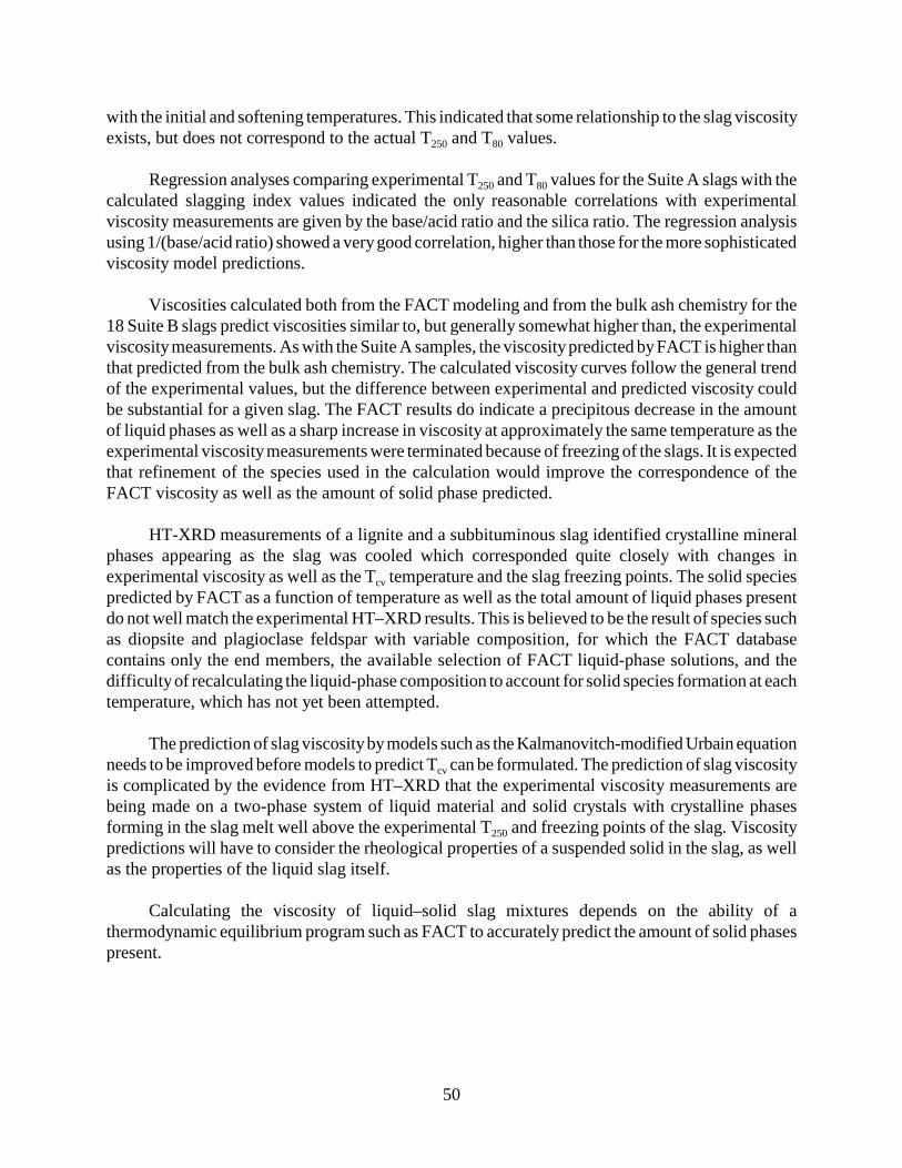
50

with the initial and softening temperatures. This indicated that some relationship to the slag viscosityexists, but does not correspond to the actual T250 and T80 values.

Regression analyses comparing experimental T250 and T80 values for the Suite A slags with thecalculated slagging index values indicated the only reasonable correlations with experimentalviscosity measurements are given by the base/acid ratio and the silica ratio. The regression analysisusing 1/(base/acid ratio) showed a very good correlation, higher than those for the more sophisticatedviscosity model predictions.

Viscosities calculated both from the FACT modeling and from the bulk ash chemistry for the18 Suite B slags predict viscosities similar to, but generally somewhat higher than, the experimentalviscosity measurements. As with the Suite A samples, the viscosity predicted by FACT is higher thanthat predicted from the bulk ash chemistry. The calculated viscosity curves follow the general trendof the experimental values, but the difference between experimental and predicted viscosity couldbe substantial for a given slag. The FACT results do indicate a precipitous decrease in the amountof liquid phases as well as a sharp increase in viscosity at approximately the same temperature as theexperimental viscosity measurements were terminated because of freezing of the slags. It is expectedthat refinement of the species used in the calculation would improve the correspondence of theFACT viscosity as well as the amount of solid phase predicted.

HT-XRD measurements of a lignite and a subbituminous slag identified crystalline mineralphases appearing as the slag was cooled which corresponded quite closely with changes inexperimental viscosity as well as the Tcv temperature and the slag freezing points. The solid speciespredicted by FACT as a function of temperature as well as the total amount of liquid phases presentdo not well match the experimental HT–XRD results. This is believed to be the result of species suchas diopsite and plagioclase feldspar with variable composition, for which the FACT databasecontains only the end members, the available selection of FACT liquid-phase solutions, and thedifficulty of recalculating the liquid-phase composition to account for solid species formation at eachtemperature, which has not yet been attempted.

The prediction of slag viscosity by models such as the Kalmanovitch-modified Urbain equationneeds to be improved before models to predict Tcv can be formulated. The prediction of slag viscosityis complicated by the evidence from HT–XRD that the experimental viscosity measurements arebeing made on a two-phase system of liquid material and solid crystals with crystalline phasesforming in the slag melt well above the experimental T250 and freezing points of the slag. Viscositypredictions will have to consider the rheological properties of a suspended solid in the slag, as wellas the properties of the liquid slag itself.

Calculating the viscosity of liquid–solid slag mixtures depends on the ability of athermodynamic equilibrium program such as FACT to accurately predict the amount of solid phasespresent.

51

REFERENCES

1. Jones, M.L.; Kalmanovitch, D.P.; Steadman, E.N.; Zygarlicke, C.J.; Benson, S.A. Applicationof SEM Techniques to the Characterization of Coal and Coal Ash Products. In Advances inCoal Spectroscopy; Meuzelaar, M.L.C., Ed.; Plenum Publishing Corp.: New York, 1992;Chapter 1, pp 1–27.

2. Skorupska, N.M.; Carpenter, A.M. Computer-Controlled Scanning Electron Microscopy ofMinerals in Coal. In Perspectives; International Energy Agency Coal Research, IEAPER/07,1993; p 21.

3. Zygarlicke, C.J.; Steadman, E.N. Advanced SEM Techniques to Characterize Coal Minerals.Scan. Electron Microsc. 1990, 4 (3), 579–590.

4. Chase, M.W.. JANAF Thermochemical Tables, 3rd ed.; American Chemical Society:Washington, DC, 1986.

5. Dow Chemical Company, Thermal Research Laboratory. JANAF Thermochemical Tables, 2nded.; U.S. National Bureau of Standards: Washington, DC, 1971.

6. Chase, M.W. JANAF Thermochemical Tables. American Chemical Society: Washington, DC,1986.

7. Dow Chemical Company Thermal Research Laboratory. JANAF Thermochemical Tables, 2nded.; Stull, D.R.; Prophet, H, project directors. U.S. National Bureau of Standards: Washington,DC, 1971.

8. Van Krevelan, D.W. Coal; Elsevier: Amsterdam, 1993.

9. Streeter, R.C. Slag Viscosity Determination; Final Report (Jan 1 – Dec 31, 1983);DOE/FC/10159-1(DE85004459), Aug 1984.

10. Bale, C.W.; Pelton, A.D.; Thompson, W.T., FACT 2.1 User Manual; Ecole Polytechnique deMontreal/Royal Military College: Canada, 1996.

11. Kalmanovitch, D.P.; Frank, M. An Effective Model of Viscosity for Ash DepositionPhenomena. In Proceedings of Mineral Matter and Ash Deposition from Coal; Bryers, R.W.;Vorres, K.S., Eds.; 1989.

12. Sage, W.L.; McIlroy, J.B. Relationship of Coal Ash Viscosity to Chemical Composition. J.Eng. Power 1960, 82 (4).

13. Hoy, H.R.; Roberts; Wilkins, D.M. Behavior of Mineral Matter in Slagging GasificationProcesses. Jour. Inst. Gas Engrs. 1965, 5, 444.

52

14. Watt, J.D. The Physical and Chemical Behavior in Coal Mineral Matter under the ConditionsMet in Combustion Plant. BCURA, Leatherhead, Surry, England, AWC, 1969.

15. Bompkamp. Development, Testing, and Evaluation of MHD Materials; NBS QuarterlyReports, Nos. 1–5, Contract No. E(49-18)-1230, 1976.

16. Schobert, H.H. Lignites of North America. Elsevier: New York, 1990; pp 89–101.

17. Senior, C.L.; Srinivasachar, S. Viscosity of Ash Particles in Combustion Systems forPrediction of Particle Sticking. Energy Fuels, 1998, 9, (2), 277–283.

18. Laumb, J.D.; Benson, S.A.; Katrinak, K.K.; McCollor, D.P. Predicting Slag Viscosity fromCoal Ash Composition. Presented at the Pittsburgh Coal Conference, 1999.

19. Urbain, G.; Cambier, F.; Deletter, M.; Anseau, M.R. Trans. J. British Ceram. Soc. 1981, 80.

20. Jung, B. Viscous Sintering of Coal Ashes in Combustion Systems. Ph.D. Dissertation,Pennsylvania State University, 1990.

21. Bryers, R.W. Fireside Slagging, Fouling, and High-Temperature Corrosion of Heat-TransferSurface Due to Impurities in Steam-Raising Fuels. Prog. Energy Combust. Sci. 1996, 22, 29.

22. Reid, W.T.; Cohen, P. The Flow Characteristics of Coal Ash Slags in the Solidification Range.J. Eng. Power Trans. ASME, Series A 1945, 66, 83.

23. Stultz, S.C.; Kitto, J.B. Steam: Its Generation and Use. Babcock and Wilcox: Barberton, OH,1992.

24. Attig, R.C.; Duzy, A.F. Coal Ash Deposition Studies and Application to Boiler Design. Am.Power Conference: Chicago, IL, Illinois Institute of Technology, 1969.

25. Bryers, R.W. Fireside Slagging, Fouling, and High-Temperature Corrosion of Heat-TransferSurface Due to Impurities in Steam-Raising Fuels. Prog. Energy Combust. Sci. 1996, 22, 29.

26. Dingwell, D.B. Sheer Viscosity of Alkali and Alkaline Earth Titanium Silicate Liquids. Am.Mineralogist 1992, 77, 270–274.

27. Stein, D.J.; Spera, F.J. Experimental Rhenometry of Melts and Supercooled Liquids in theSystem NaAlSiO4–SiO2: Implications for Structure and Dynamics. Am. Mineralogist 1993, 78,710–723.

28. Toplis, M.J.; Dingwell, D.B.; Hess, K.U.; Lenci, T. Viscosity, Fragility, and ConfigurationalEntropy of Melts Along the Join SiO2–NaAlSiO4. Am. Mineralogist 1997, 82, 979–990.

53

29. Baker, D.R. Granitic Melt Viscosity: Empirical and Configurational Entropy Models For TheirCalculation. Am. Mineralogist 1996, 81, 126–134.

30. Dingwell, D.B.; Hess, K.U.; Romano, C. Viscosities of Granitic (sensu lato): Influence of theAnorthite Component. Am. Mineralogist 2000, 85, 1342–1348.

31. Bottinga, Y; Richet, P.; Sipp, A. Viscosity Regimes of Homogenous Silicate Melts. Am.Mineralogist 1995, 80, 305–318.

32. Hess, K.U.; Dingwell, D.B. Viscosities of Hydrous Leucogranitic Melts: A Non-ArrhenianModel. Am. Mineralogist 1996, 81, 1297–1300.

33. Doremus, R.H. Water Speciation in Silicate Glasses and Melts: Langmuir Limited Site Model.Am. Mineralogist. 2000, 85, 1674–1680.

34. Kroeker, S.; Stebbins, J.F. Magnesium Coordination Environments in Glasses and Minerals:New Insights from High-Field Magnesium-25 MAS NMR. Am. Mineralogist 2000, 85,1459–1464.

35. Stebbins, J.F.; Sen, S.; Farnan, I. Silicate Species Exchange, Viscosity, and Crystallization ina Low-Silica Melt: In Situ High-Temperature MAS NMR Spectroscopy. Am. Mineralogist1995, 80, 861–864.

36. Stebbins, J.F.; Oglesby, J.V.; Xu, Z. Disorder Among Network-Modifier Cations in SilicateGlasses: New Constraints from Triple-Quantum 17O NMR. Am. Mineralogist 1997, 82,1116–1124.

37. Folkedahl, B.C. A Study of the Viscosity of Coal Ash and Slag. Ph.D. Dissertation,Pennsylvania State University, 1997.

38. Hough, D.C.; Sanyal, A.; Annen, K.D.; Gruninger, J.H; Stewart, G.W. The Development ofan Improved Coal Ash Viscosity/Temperature Relationship for the Assessment of SlaggingPropensity in Coal-Fired Boilers. J. Inst. Energy 1986, 59, 77–81.

APPENDIX A

EXAMPLE OF OUTPUT FOR ASHTRANSFORMATION MODEL

ENTRAINED FLY ASHPREDICTED FROM ADVANCED COAL ANALYSIS

AERO. DIAMETER 0.0-1.0 1.0-3.0 3.0-10.0 10.0-30.0 30.0-50.0 UNUSED Tot.QUARTZ 0.00 0.00 0.00 0.00 0.00 0.00 0.00IRON OXIDE 0.00 0.00 0.00 0.00 0.00 0.00 0.00PERICLASE 0.00 0.00 0.00 0.00 0.00 0.00 0.00RUTILE 0.00 0.00 0.00 0.67 0.00 0.00 0.67ALUMINA 0.00 0.00 0.00 0.00 0.00 0.00 0.00CALCITE 0.00 0.00 0.10 0.04 0.00 0.00 0.14DOLOMITE 0.00 0.00 0.04 0.00 0.00 0.00 0.04ANKERITE 0.00 0.01 1.25 0.50 0.00 0.00 1.76KAOLINITE 0.00 0.00 0.00 0.00 0.00 0.00 0.00MONTMORILLONITE 0.00 0.00 0.00 0.00 0.00 0.00 0.00K AL-SILICATE 0.00 0.00 0.00 0.00 0.00 0.00 0.00FE AL-SILICATE 0.00 0.00 0.00 0.00 0.00 0.00 0.00CA AL-SILICATE 0.00 0.00 1.52 6.67 0.00 0.00 8.19NA AL-SILICATE 0.00 0.00 0.00 0.00 0.00 0.00 0.00ALUMINOSILICATE 0.00 0.00 0.00 0.00 0.00 0.00 0.00MIXED AL-SILICATES 0.00 0.00 0.00 0.08 0.00 0.00 0.08FE SILICATE 0.00 0.00 0.00 0.00 0.00 0.00 0.00CA SILICATE 0.00 0.00 9.23 12.13 0.00 0.00 21.36CA ALUMINATE 0.00 0.00 0.10 0.01 0.00 0.00 0.11PYRITE 0.00 0.00 0.00 0.00 0.00 0.00 0.00PYRRHOTITE 0.00 0.00 0.00 0.00 0.00 0.00 0.00OXIDIZED PYRRHOTITE 0.00 0.00 0.00 0.00 0.00 0.00 0.00GYPSUM 0.00 0.00 0.00 0.00 0.00 0.00 0.00BARITE 0.00 0.00 0.00 0.00 0.00 0.00 0.00APATITE 0.00 0.00 0.00 0.00 0.00 0.00 0.00CA AL-P 0.00 0.00 0.27 0.46 0.00 0.00 0.72KCL 0.00 0.00 0.00 0.00 0.00 0.00 0.00GYPSUM/BARITE 0.00 0.00 0.00 0.00 0.00 0.00 0.00GYPSUM/AL-SILICATE 0.00 0.00 0.00 0.00 0.00 0.00 0.00SI-RICH 0.00 0.00 0.00 0.00 0.00 0.00 0.00CA-RICH 0.00 1.05 0.62 0.00 0.00 0.00 1.66CA-SI RICH 0.00 0.00 0.33 0.44 0.00 0.00 0.76UNKNOWN 0.00 0.02 17.94 16.34 0.45 0.00 34.75TOTAL 0.00 1.07 31.39 37.33 0.45 0.00 70.24

NUCLEATED FLY ASH AVERAGE COMPOSITION(OxIDES)NA2O MGO AL2O3 SIO2 P2O5 SO3 CL2O7 K2O CAO FE2O3 BAO TIO21.60 2.90 12.00 10.90 0.00 0.00 0.00 1.10 54.60 14.70 0.00 2.30

BULK COMPOSITION OF FLYASH AS OXIDESNA2O MGO AL2O3 SIO2 P2O5 SO3 CL2O7 K2O CAO FE2O3 BAO TIO21.7 6.6 15.5 25.3 0.5 0.0 0.0 0.7 38.1 9.9 0.0 1.6

BULK COMPOSITION OF < 1.0 MICRON ASHWEIGHT PERCENT 9.52NA2O MGO AL2O3 SIO2 P2O5 SO3 CL2O7 K2O CAO FE2O3 BAO TIO21.6 2.9 12.0 10.9 0.0 0.0 0.0 1.1 54.6 14.7 0.0 2.3

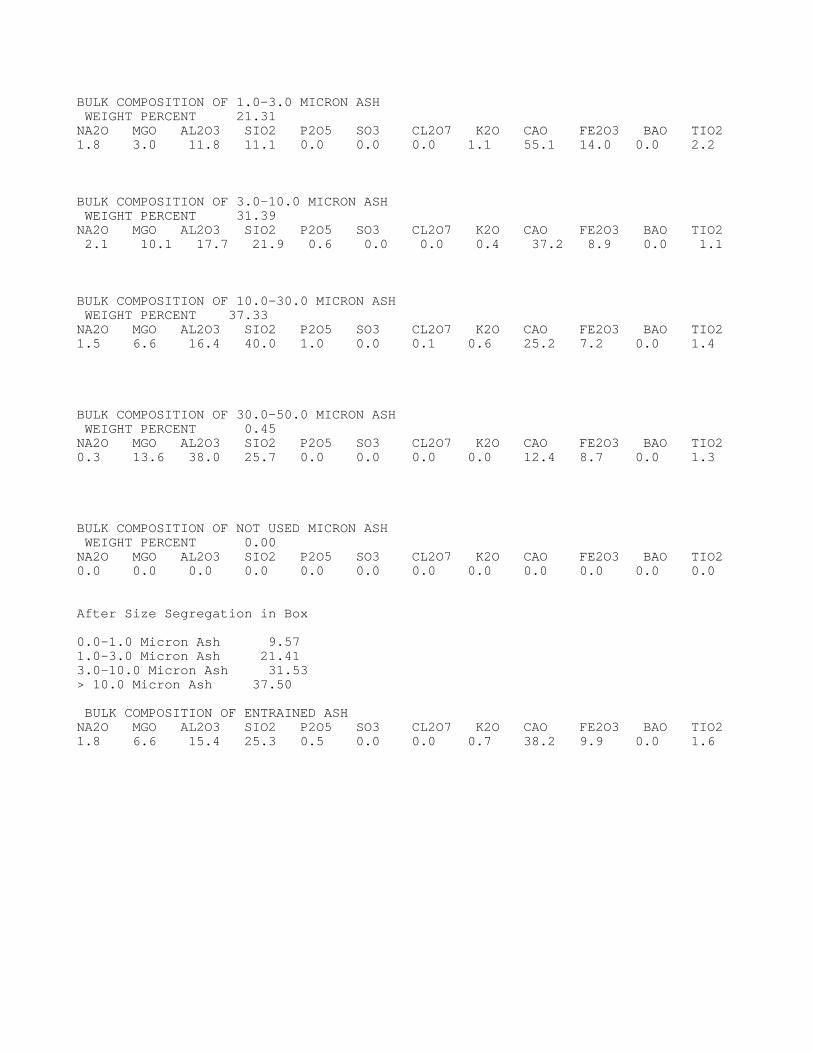
BULK COMPOSITION OF 1.0-3.0 MICRON ASHWEIGHT PERCENT 21.31NA2O MGO AL2O3 SIO2 P2O5 SO3 CL2O7 K2O CAO FE2O3 BAO TIO21.8 3.0 11.8 11.1 0.0 0.0 0.0 1.1 55.1 14.0 0.0 2.2




BULK COMPOSITION OF NOT USED MICRON ASHWEIGHT PERCENT 0.00NA2O MGO AL2O3 SIO2 P2O5 SO3 CL2O7 K2O CAO FE2O3 BAO TIO20.0 0.0 0.0 0.0 0.0 0.0 0.0 0.0 0.0 0.0 0.0 0.0

After Size Segregation in Box

0.0-1.0 Micron Ash 9.571.0-3.0 Micron Ash 21.413.0-10.0 Micron Ash 31.53> 10.0 Micron Ash 37.50

BULK COMPOSITION OF ENTRAINED ASHNA2O MGO AL2O3 SIO2 P2O5 SO3 CL2O7 K2O CAO FE2O3 BAO TIO21.8 6.6 15.4 25.3 0.5 0.0 0.0 0.7 38.2 9.9 0.0 1.6

APPENDIX B

EXAMPLE OF THETRACE ELEMENT OUTPUT FILE

TRACE ELEMENT COMPOSITION PPM/Size Range

As Cd Cr Pb Ni Se Hg %AshVapor 0.0 0.0 0.0 0.0 0.0 11.1 0.71 < 128.1 31.7 341.4 246.0 769.4 122.4 0.0 6.71.0-3.0 30.3 7.5 90.0 61.5 183.3 30.6 0.0 3.23.0-10.0 3.2 0.6 110.2 13.3 47.8 6.6 0.0 20.910.0-30.0 5.7 1.0 240.2 22.1 99.8 10.9 0.0 59.830.0-50.0 4.7 0.8 188.8 18.6 79.3 9.2 0.0 9.4>50 0.0 0.0 0.0 0.0 0.0 0.0 0.0 0.0Bulk 14.1 3.2 210.1 36.1 134.4 21.5 0.2

TRACE ELEMENT COMPOSITION PPM/Total Ash

As Cd Cr Pb Ni Se HgVapor 0.0 0.0 0.0 0.0 0.0 11.1 0.71 < 8.6 2.1 22.8 16.4 51.4 8.2 0.01.0-3.0 1.0 0.2 2.9 2.0 6.0 1.0 0.03.0-10.0 0.7 0.1 23.0 2.8 10.0 1.4 0.010.0-30.0 3.4 0.6 143.6 13.2 59.6 6.5 0.030.0-50.0 0.4 0.1 17.8 1.8 7.5 0.9 0.0>50 0.0 0.0 0.0 0.0 0.0 0.0 0.0Bulk 14.1 3.2 210.1 36.1 134.4 21.5 0.2

ENTRAINED FLY ASHPREDICTED FROM ADVANCED COAL ANALYSIS

As Cd Cr Pb Ni Se Hg Total------------------------------------------------------------------------------

QUARTZ 0.0 0.0 0.3 0.1 0.2 0.0 0.0 0.6IRON OXIDE 0.1 0.0 47.0 0.4 16.7 0.2 0.0 64.5PERICLASE 0.0 0.0 0.0 0.0 0.0 0.0 0.0 0.0RUTILE 0.0 0.0 0.0 0.0 0.0 0.0 0.0 0.0ALUMINA 0.0 0.0 0.0 0.0 0.0 0.0 0.0 0.0CALCITE 0.0 0.0 0.0 0.0 0.0 0.0 0.0 0.1DOLOMITE 0.0 0.0 0.0 0.0 0.0 0.0 0.0 0.0ANKERITE 0.0 0.0 0.3 0.0 0.1 0.0 0.0 0.4KAOLINITE 0.0 0.0 0.4 0.0 0.1 0.0 0.0 0.6MONTMORILLONITE 0.0 0.0 0.2 0.0 0.1 0.0 0.0 0.2K AL-SILICATE 0.0 0.0 0.4 0.0 0.1 0.0 0.0 0.6FE AL-SILICATE 1.3 0.2 44.1 4.9 18.8 2.4 0.0 71.7CA AL-SILICATE 0.0 0.0 0.0 0.0 0.0 0.0 0.0 0.0NA AL-SILICATE 0.0 0.0 0.0 0.0 0.0 0.0 0.0 0.0ALUMINOSILICATE 0.0 0.0 0.1 0.0 0.0 0.0 0.0 0.1MIXED AL-SILICATES 0.0 0.0 1.7 0.1 0.6 0.1 0.0 2.5FE SILICATE 0.1 0.0 3.8 0.5 1.7 0.2 0.0 6.4CA SILICATE 0.0 0.0 0.0 0.0 0.0 0.0 0.0 0.0CA ALUMINATE 0.0 0.0 0.0 0.0 0.0 0.0 0.0 0.1PYRITE 0.0 0.0 6.5 0.1 2.2 0.1 0.0 9.0PYRRHOTITE 0.0 0.0 1.4 0.1 0.5 0.1 0.0 2.2OXIDIZED PYRRHOTITE 0.0 0.0 2.7 0.1 1.0 0.1 0.0 3.9GYPSUM 0.0 0.0 0.0 0.0 0.0 0.0 0.0 0.0BARITE 0.0 0.0 0.0 0.0 0.0 0.0 0.0 0.0APATITE 0.0 0.0 0.0 0.0 0.0 0.0 0.0 0.0CA AL-P 0.0 0.0 0.0 0.0 0.0 0.0 0.0 0.0KCL 0.0 0.0 0.0 0.0 0.0 0.0 0.0 0.0GYPSUM/BARITE 0.0 0.0 0.0 0.0 0.0 0.0 0.0 0.0GYPSUM/AL-SILICATE 0.0 0.0 0.0 0.0 0.0 0.0 0.0 0.0SI-RICH 0.2 0.0 2.1 0.9 1.5 0.4 0.0 5.1CA-RICH 0.0 0.0 0.4 0.1 0.2 0.1 0.0 0.9CA-SI RICH 0.0 0.0 0.0 0.0 0.0 0.0 0.0 0.0UNKNOWN 2.6 0.5 82.7 10.1 36.5 5.0 0.0 137.3TOTAL 4.5 0.8 194.3 17.6 80.4 8.7 0.0 306.4

NUCLEATED FLY ASH AVERAGE COMPOSITION, PPMAs Cd Cr Pb Ni Se Hg9.5 2.4 25.3 18.2 57.0 9.1 0.0

APPENDIX C

PAPER WITH ADDITIONAL TESTING RESULTS

Predicting Ash Particle Size and Composition Distribution Produced During Pulverized-Coal Combustion

Steven A. BensonEnergy & Environmental Research CenterUniversity of North DakotaPO Box 9018Grand Forks, ND 58202, USAE-Mail: [email protected]; Telephone: (701)777-5177, Fax: (701)777-5181

Abstract No. ABS.338The size and composition of ash particles produced during pulverized-coal combustion have a major impact on their fate incombustion systems. The size and composition of the ash influence the formation of ash deposits and the performance ofparticulate control devices. An ash transformation model, Atran, was developed at the Energy & Environmental ResearchCenter (EERC) to predict the size and composition of ash particles and is used in other computer models to predict ashdeposition in combustion systems. The inputs to the model include size, composition, and abundance of mineral grains in thecoal as determined by computer-controlled scanning electron microscopy; bulk ash composition; ultimate analysis; andabundance of inorganic elements organically associated. Processes such as vaporization/condensation, ash mineralcoalescence, partial coalescence, ash shedding, and char fragmentation during char combustion and mineral fragmentationhave been incorporated into the model and all play an important role in the size and composition of the final fly ash. The sizeand composition distribution of the entrained ash produced from lignite, subbituminious, and bituminous coals in full-, pilot-,and laboratory-scale combustion systems have been compared to the predictions made with Atran. The entrained ash wascollected and aerodynamically classified. The sized fractions were analyzed to determine chemical compositions. Theparticle-size and composition distributions for 6000 particles for each coal were calculated using Atran and then binned bysize and composition for comparison with ash collected. The model predictions and actual measurements compared veryfavorably.

IntroductionInorganic coal components undergo complex chemical and physical transformations during combustion to produce vapors,liquids, and solids in the combustion system. The partitioning of the inorganic components during combustion to formvapors, liquids, and solids depends upon the association and chemical characteristics of the inorganic components, thephysical characteristics of the coal particles, the physical characteristics of the coal minerals, and the combustion conditions.The physical transformation of inorganic constituents depends on the inorganic composition of the coal and combustionconditions. The inorganic components can consist of organically associated cations, mineral grains that are included in coalparticles, and excluded mineral grains. There is a wide range of combinations of mineral–mineral, mineral–coal,mineral–cation–coal, and mineral–mineral–cation–coal associations in coal. These associations are unique to each coalsample. The physical transformations involved in fly ash formation include 1) coalescence of individual mineral grainswithin a char particle, 2) shedding of the ash particles from the surface of the chars, 3) incomplete coalescence due todisintegration of the char, 4) convective transport of ash from the char surface during devolatilization, 5) fragmentation ofthe inorganic mineral particles, 6) formation of cenospheres, and 7) vaporization and subsequent condensation of theinorganic components upon gas cooling. Combustion conditions and temperature profiles in the boiler will influence thephysical transformation mechanisms involved in ash formation. As a result of these interactions, the ash size distribution isgenerally bimodal, with the submicron component largely a result of the condensation of the flame-volatilized inorganiccomponent and the supermicron fraction being from the mineral grains combined with cations (Loehden and others, 1989; Zygarlicke and others, 1990). Numerous studies have been conducted to quantify the physical transformation mechanisms(Benson and others, 1993b).

The ash transformation model (Atran) was developed to predict the size and composition of ash particles produced duringcoal combustion. The code has been described in detail by Hurley and coworkers (1992). Atran is a key component in othermodels developed at the Energy & Environmental Research Center (EERC), including TraceTran and Fuel Quality Advisor(FQA). TraceTran was developed based on Atran to predict particle-size and composition distributions (PSCD) of major,minor, and trace elements of interest in combustion and gasification systems (Erickson and others, 1998). The Tracetranmodel was designed for a gasification system and will predict trace elements. FQA is used to predict high- and

low-temperature convective pass fouling behavior. The code provides deposit growth rates, deposit removability, and effectson heat transfer (Benson and others, 1993a).

This paper describes tests conducted with the Atran code to optimize key input information such as combustion parametersthat will influence fragmentation and coalescence of minerals and heterogeneous and homogeneous interaction of organicallyassociated cations. A Powder River Basin (PRB) subbituminous coal from the Rochelle Mine was combusted in theconversion and environmental process simulator (CEPS), and the ash produced was collected and aerodynamically sized,with each size fraction being analyzed for major and minor element composition. The information was then compared to thepredicted results from the ash transformation model.

Experimental MethodsThe Atran model requires computer-controlled scanning electron microscopy (CCSEM), x-ray fluorescence (XRF), andultimate analysis of the fuel and boiler design and operating parameters in order to predict the size and compositiondistribution of the ash. In this study, Rochelle coal was analyzed to determine the size, composition, abundance, andassociation of mineral grains using CCSEM (Zygarlicke and Steadman, 1990); bulk ash composition by XRF; and C, H, N,O, and S by ultimate analysis. The CCSEM analysis is also combined with a locked/liberated particle analysis to determine ifthe individual mineral grains are located within a coal matrix or are free mineral grains.

The ash was produced in the CEPS combustion system when firing Rochelle coal. The CEPS is pilot-scale combustordesigned to nominally top-fire pulverized coal, with a heat input of 40,000 Btu/hr. The CEPS was operated at a coal feed rateof 1.4 kg/hour, 25% excess air, a 1500°C initial combustion temperature, and an 1100°C convective pass inlet temperature. Aportion of the particulate was removed before the convective pass section of the CEPS. The fly ash was sampled using asource assessment sampling system (SASS) train. The SASS train is equipped with three cyclones and a backup filter used toaerodynamically classify the ash into the following size fractions < 1, 1–3, 3–10, and 10–50 micrometers.

Coal composition, boiler design, and operating conditions were used as input parameters into the Atran model to determinethe size partitioning of the inorganic species during fly ash formation for Rochelle coal. With these inputs, the Atran modelbegins by calculating a mass balance on the inorganic composition by comparing the CCSEM mineral composition and bulkash composition data. The balance provides the compositions of locked minerals (in the coal matrix) and liberated minerals(outside the coal matrix) and type and abundance of organically associated constituents. Once the mass balance is complete,the distribution of the cations for homogeneous and heterogeneous condensation and interaction and the degree offragmentation and coalescence of mineral grains are defined based on boiler design and operating conditions. The boilerdesign and operating conditions specifically define a file called "homohet" that is used to determine the percentage of themajor elements (Na, Mg, Al, Si, P, K, Ca, Ti, and Fe), which is distributed between homogeneous and heterogeneous alongthe percentage of the homogeneously nucleated particles that are submicron. The organically associated cations go through avaporization step and then are split between heterogeneous condensation and homogeneous condensation. The heterogeneouscondensation step distributes the particles into the supermicron fly ash size bins along with the homogeneous condensationagglomerations. The remaining homogeneous condensation particles are distributed into the submicron fly ash size bins.Boiler design and operational parameters are linked to fragmentation and coalescence factors for mineral grains, includingpyrite, iron carbonate, pyrrhotite, gypsum, barite, Ca–Al–P, kaolinite, dolomite, and quartz. A fragmentation is then appliedto both the locked and liberated particles. Coalescence and shedding are applied to the locked particles before theheterogeneous condensation stage. The liberated particles go directly into the heterogeneous condensation step. The ash isthen partitioned and run through a mass balance calculation to yield a predicted PSCD. The homogeneous/heterogeneous andfragmentation/coalescence values need to be optimized for specific boiler designs and operating conditions.

Results and DiscussionThe homogeneous/heterogeneous and fragmentation/coalescence values were optimized and used in Atran to predict thePSCD of the ash produced from Rochelle coal. The predicted results are compared with the measured composition of theaerodynamically classified particles produced upon combustion of the Rochelle coal as shown in Figure 1. Atran alsopredicts the weight percent of ash in the various size fractions and is shown in Figure 2. In general, the SiO2 levels in thevarious size fractions compare well with the predicted values for all size fractions. The predicted CaO levels compare wellwith the predicted values for the <10-micrometer size fractions. The CaO content in the >10-micrometer-sized ash particleswas found to be higher than the predicted. The higher level of CaO may be due to the loss of larger particles in the CEPS

Figure 2. Comparison of the predicted mass in the various sizefractions.

Figure 1. Comparison of the composition of the predicted and measured ash compositions.

after the gas stream passes through the convective pass or may be due to underpredicting the interaction of the organicallyassociated calcium with the coalescing mineral during combustion. Differences were also noted between the predicted andmeasured Al2O3 contents. The differences may be due to the fact that some of the aluminum in PRB coals is associated as amineral that is composed of high levels of calcium, aluminum, and phosphorus similar in composition to crandalite. Theexact transformations of crandalite have not yet been established. The Fe2O3 content compares well with the particles>3 micrometers; however, for the smaller particles, Atran is overestimating the levels of Fe2O3.

The predicted size distribution shows some differences for the two larger-size fractions of ash and good agreement for thesmaller sizes. The primary reason for the differences is likely due to the loss of some of the larger particles in the CEPS asthe particles enter the convective pass of the furnace.

Conclusions The homogeneous/heterogeneous and fragmentation/coalescence values must be optimized for various firing systems andfiring conditions. The predicted results compared with the measured composition of the aerodynamically classified particlesproduced upon combustion of the Rochelle coal show generally good agreement. The SiO2 levels in the various size fractionscompare well with the predicted values for all size fractions. The predicted CaO levels compare well with the predictedvalues for the <10-micrometer-size fractions. The CaO content in the >10-micrometer-sized ash particles was found to behigher than the predicted. Differences were also noted between the predicted and measured Al2O3 contents. The Fe2O3content compares well with the particles >3 micrometers; however, for the smaller particles, Atran is overestimating thelevels of Fe2O3. The predicted size distribution shows some differences for the two larger-size fractions of ash and goodagreement for the smaller sizes. The primary reason for the differences is likely due to the loss of some of the larger particlesin the CEPS as the particles enter the convective pass of the furnace.

ReferencesBenson, S.A.; Hurley, J.P.; Zygarlicke, C.J.; Steadman, E.N.; Erickson, T.A. Predicting Ash Behavior in Utility Boilers.Energy Fuels 1993a, 7, 746–754.

Benson, S.A.; Jones, M.L.; Harb, J.N. Ash Formation and Deposition. In Fundamentals of Coal Combustion for Clean andEfficient Use; Smoot, L.D., Ed.; Elsevier: New York, 1993b; pp 299–374.

Erickson, T.A.; Galbreath, K.C.; Zygarlicke, C.J.; Hetland, M.D.; Benson, S.A. Trace Element Emissions Project; FinalTechnical Progress Report (Aug 1992 – Dec 1998) for U.S. Department of Energy Contract No. DE-AC21-92MC28016;Energy & Environmental Research Center: Grand Forks, ND, Oct 1998.

Hurley, J.P.; Benson, S.A.; Erickson, T.A.; Allan, S.E.; Bieber, J.A. Project Calcium; Final Report; Energy & EnvironmentalResearch Center: Grand Forks, ND, 1992. Loehden, D.; Walsh, P.M.; Sayre, A.N.; Beer, J.M.; Sarofim, A.F. Generation and Deposition of Fly Ash in the Combustionof Pulverized Coal. J. Inst. Energy 1989, 119–127.

Zygarlicke, C.J.; Toman, D.L.; Benson, S.A. Trends in the Evolution of Fly Ash Size During Combustion. Prepr. Pap.—Am.Chem. Soc., Div. Fuel Chem. 1990, 35 (3), 621–636.

Zygarlicke, C.J.; Steadman, E.N. Advanced SEM Techniques to Characterize Coal Minerals. Scan. Electron Microsc. 1990,4 (3), 579–590.

Contributing AuthorsThomas A. Erickson, Robert R. Jensen, and Jason D. LaumbAffiliation: Energy & Environmental Research Center, University of North DakotaPO Box 9018, Grand Forks, ND 58202-9018 USA

advanced power systems analysis tools - digital library/67531/metadc717935/m2/1/high... · subtask...

Documents