advanced ndt methods and data processing on industrial

applied sciences

Article

Advanced NDT Methods and Data Processing onIndustrial CFRP Components

Vito Dattoma, Francesco Willem Panella *, Alessandra Pirinu and Andrea Saponaro

Department of Engineering, University of Salento, 73100 Lecce, Italy; [email protected] (V.D.);[email protected] (A.P.); [email protected] (A.S.)* Correspondence: [email protected]; Tel.: +39-0832-297771

Received: 28 November 2018; Accepted: 14 January 2019; Published: 24 January 2019��

Abstract: In this work, enhanced thermal data processing is developed with experimental procedures,improving visualization algorithm for sub-surface defect detection on industrial composites.These materials are prone to successful infrared nondestructive investigation analyses, since defectsare easily characterized by temperature response under thermal pulses with reliable results.Better defect characterization is achieved analyzing data with refined processing and experimentalprocedures, providing detailed contrasts maps where defects are better distinguished. Thermal dataare analyzed for different CFRP specimens with artificial defects and experimental procedures areverified on real structural aeronautical component with internal anomalies due to impact simulation.A better computation method is found to be useful for simultaneous defect detection by means ofautomatic mapping of absolute contrast, optimized to identify defect boundaries.

Keywords: aeronautical component; CFRP; nondestructive testing; pulsed thermography; artificialdefects; thermal contrast; ultrasonic method

1. Introduction

Internal defects are the major sources of composite failures in FRP structures and originate frommanufacturing (delamination, voids, porosity, fiber wrinkles, etc.) and/or from in-service events(impact or fatigue damage, micro-cracks, debonding, delamination, erosion, etc.). A combination ofcontemporaneous voids, matrix cracks, and multiple delamination may occur, and structural integrityis verified using nondestructive testing (NDT) methods to determine the damage risk [1].

Thermal methods are most effective for thin laminates or for defects near the surface and thepassive or active approach are adopted. In active IRT methods, an external stimulus is applied tospecimen surface, in order to induce relevant thermal contrasts between regions of interest and thesetechniques include pulsed thermography (PT) as valid robust technique for checking the integrityof structures [2,3] and consists of rapidly heating the specimen recording the temperature decaycurve; the free-defect material conducts heat more efficiently than defective zones, where heat is eitherabsorbed, or reflected, indicating the quality state of the inspected area [4].

Active IR-thermographic methods such as cooling down thermography (CDT) [5] or long pulsedthermography (LPT) [6,7] give satisfactory results for similar defects in composites. In this paper,PT thermography in the range of long pulses is explored, even that heat accumulation phenomenonmay occur for subsurface defects. The CDT method represents an interesting and valid ND approachwhere a previous thermal excitation in an oven allows a uniform temperature through thickness andcould be applied on CFRP plates, especially in the case of deeper defects.

However, this is not a suitable technique for wider structural component of the authors’ lack ofexperience and need of a large climatic chamber. However, future CDT tests will be considered.

Appl. Sci. 2019, 9, 393; doi:10.3390/app9030393 www.mdpi.com/journal/applsci

http://www.mdpi.com/journal/applsci

http://www.mdpi.com

https://orcid.org/0000-0003-1363-4291

http://www.mdpi.com/2076-3417/9/3/393?type=check_update&version=1

http://dx.doi.org/10.3390/app9030393

http://www.mdpi.com/journal/applsci

Appl. Sci. 2019, 9, 393 2 of 17

Raw thermal imaging from PT investigation is usually not suitable for a precise material evaluationand a quantitative analysis of the registered temperatures is required to better determine the dimension,depth, and defect shape. Signal levels associated with subsurface anomalies can be lost in the thermaldata noise [8] and proper different post-processing methods are used to improve the signal-to-noise(SNR) content of recorded data.

Several processing methods have been developed to improve delamination characterization forthermographic tools [9] and introduce automatic images analysis, actual main goal for thermographicinspection, providing a pass-or-fail diagnostic to the operator [10,11]. The literature on thermalimage-processing proposes different algorithms developed to improve detect detection from thermalmaps [3,12] and, in the present paper, a different image-processing method is introduced, where defectsare automatically visualized on thermal contrast maps for CFRP specimens and experimentalprocedure is optimized, in order to facilitate inspections for operators with automatic and accuratepost-processing, at the same time with good reliability level to be guaranteed.

Since thermography is considered as an emerging technology, real component thermal contrastmaps were verified using the well-established ultrasonic c-scanning technique, as explained in otherworks [13] for unknown damage area evaluation on composites, using modern phased array probe;several authors [14–16] make use of ultrasonic NDI systems for the reliable and effective detection ofdelaminations, the primary important damage mode for aeronautical applications, where fatigue andimpact failures are likely to occur [17].

2. Materials and Methods

For the optimization and the calibration of thermal signal processing, standard specimens in theform of plates with artificial defects, built with expanded polystyrene inserts, are produced; these arecrucial to determine the detectability limits of the proposed technique [18] for defect size, depth,and type certification after inspection.

2.1. CFRP Plates and Component

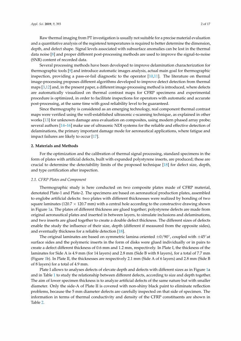
Thermographic study is here conducted on two composite plates made of CFRP material,denotated Plate-1 and Plate-2. The specimens are based on aeronautical production plates, assembledto englobe artificial defects: two plates with different thicknesses were realized by bonding of twosquare laminates (120.7 × 120.7 mm) with a central hole according to the constructive drawing shownin Figure 1a. The plates of different thickness are glued together; polystyrene defects are made fromoriginal aeronautical plates and inserted in between layers, to simulate inclusions and delaminations,and two inserts are glued together to create a double defect thickness. The different sizes of defectsenable the study the influence of their size, depth (different if measured from the opposite sides),and eventually thickness for a reliable detection [18].

The original laminates are based on symmetric lamina oriented ±0/90◦, coupled with ±45◦atsurface sides and the polymeric inserts in the form of disks were glued individually or in pairs tocreate a defect different thickness of 0.6 mm and 1.2 mm, respectively. In Plate I, the thickness of thelaminates for Side A is 4.9 mm (for 14 layers) and 2.8 mm (Side B with 8 layers), for a total of 7.7 mm(Figure 1b). In Plate II, the thicknesses are respectively 2.1 mm (Side A of 6 layers) and 2.8 mm (Side Bof 8 layers) for a total of 4.9 mm.

Plate I allows to analyses defects of elevate depth and defects with different sizes as in Figure 1aand in Table 1 to study the relationship between different defects, according to size and depth together.The aim of lower specimen thickness is to analyze artificial defects of the same nature but with smallerdiameter. Only the side-A of Plate II is covered with non-shiny black paint to eliminate reflectionproblems, because the 5 mm diameter defects are carefully inspected on that side of specimen. Theinformation in terms of thermal conductivity and density of the CFRP constituents are shown inTable 2.

Appl. Sci. 2019, 9, 393 3 of 17

Table 1. Artificial defect geometry in the plates.

Defect Nomenclature D1 D2 D3 D4 D5 D6 D7

N. Defect in Plate I 1 2 1 3 2 1 3

N. Defect in Plate II 1 2 1 3 2 1 3

Diameter (mm) 25 10 15 5 10 15 5

Thickness (mm) 0.6 0.6 0.6 0.6 1.2 1.2 1.2Appl. Sci. 2018, 8, x FOR PEER REVIEW 3 of 18

(a) (b)

Figure 1. (a) Layout of artificial defects and position. (b) Exploded Assembly of Plate I, identical for

Plate II.

The original laminates are based on symmetric lamina oriented ±0/90°, coupled with ±45°at

surface sides and the polymeric inserts in the form of disks were glued individually or in pairs to

create a defect different thickness of 0.6 mm and 1.2 mm, respectively. In Plate I, the thickness of the

laminates for Side A is 4.9 mm (for 14 layers) and 2.8 mm (Side B with 8 layers), for a total of 7.7 mm

(Figure 1b). In Plate II, the thicknesses are respectively 2.1 mm (Side A of 6 layers) and 2.8 mm (Side

B of 8 layers) for a total of 4.9 mm.

Plate I allows to analyses defects of elevate depth and defects with different sizes as in Figure 1a

and in Table 1 to study the relationship between different defects, according to size and depth

together. The aim of lower specimen thickness is to analyze artificial defects of the same nature but

with smaller diameter. Only the side-A of Plate II is covered with non-shiny black paint to eliminate

reflection problems, because the 5 mm diameter defects are carefully inspected on that side of

specimen. The information in terms of thermal conductivity and density of the CFRP constituents are

shown in Table 2.

Table 1. Artificial defect geometry in the plates

Defect Nomenclature D1 D2 D3 D4 D5 D6 D7

N. Defect in Plate I 1 2 1 3 2 1 3

N. Defect in Plate II 1 2 1 3 2 1 3

Diameter (mm) 25 10 15 5 10 15 5

Thickness (mm) 0.6 0.6 0.6 0.6 1.2 1.2 1.2

Table 2. Mechanical properties of carbon fiber and epoxy resin

Carbon Fiber

Density (g/cm3) 1.65

Areal weight (g/m2) 240

Thermal conductivity coefficient (W/mK) ~ 15

Epoxy Resin

Density (g/ml) 1.14–1.16

Young Modulus (MPa) 2900–3100

Ultimate stress (MPa) 75–80

Ultimate strain (%) 8.5–9

Thermal conductivity coefficient (W/mK) ~ 0.22

Figure 1. (a) Layout of artificial defects and position. (b) Exploded Assembly of Plate I, identical forPlate II.

Table 2. Mechanical properties of carbon fiber and epoxy resin.

Carbon Fiber

Density (g/cm3) 1.65Areal weight (g/m2) 240

Thermal conductivity coefficient (W/mK) ~ 15

Epoxy Resin

Density (g/ml) 1.14–1.16Young Modulus (MPa) 2900–3100Ultimate stress (MPa) 75–80

Ultimate strain (%) 8.5–9Thermal conductivity coefficient (W/mK) ~ 0.22

In addition, an aeronautical multi-stringer component of medium size (Dim. 914.4 × 762 mm) incarbon fiber is studied; Figure 2a shows the geometry of the structural component; CFRP laminatesare based on different ply layers (Table 3). In this component, rivets secure the ribs on the skin,while stringers are co-cured.

Appl. Sci. 2019, 9, 393 4 of 17

Appl. Sci. 2018, 8, x FOR PEER REVIEW 4 of 18

In addition, an aeronautical multi-stringer component of medium size (Dim. 914.4 × 762 mm) in

carbon fiber is studied; Figure 2a shows the geometry of the structural component; CFRP laminates

are based on different ply layers (Table 3). In this component, rivets secure the ribs on the skin, while

stringers are co-cured.

The component presents an artificial discontinuity in the center, in the form of a large cut (Dim.

152.4 × 6.35 mm) to simulate the effect of heavy impact, leading to central stiffener collapse; this

artificial damage on the central skin interrupts the stringer continuity and simulates the presence of

severe damage in whole area (Figure 2b), which is expected to produce delaminations during static

testing before failure. The information in terms of material and lamina property constituents are

shown in Table 3.

(a) (b)

Figure 2. (a) CFRP multi stringer multi-stringer component’s geometry and (b) and artificial damage

geometry.

Table 3. Part components for multi-stringer element

Part

Component

Sub-Part

Component Material

Lamina

Thickness

(mm)

N°

Plies Stacking Sequence

Skin Skin 1 CFRP 0.186 20 [45/90/−45/−45/45/90/0/-45/45/0] S

Skin 2 CFRP 0.186 24 [45/90/0/0/−45/−45/45/90/0/−45/45/0] S

Stringer CFRP 0.186 12 [45/90/0/0/−45/0] S

Rib CFRP 0.208 12 [45/0/−45/90/45/0] S

2.2. Experimental Setup and Inspection Methods

Pulsed thermographic tests have been conducted with long pulses in the experimental

laboratory located in the Engineering Faculty of the University of Salento (Lecce, Italy).

Thermographic set-up means both the equipment used to test and the appropriate arrangement of

specimen position and excitation are influent on results [19].

The equipment consists of an array of four halogen lamps, each of 1000 W, controlled by a signal

generator with single square wave form of amplitude set to maximum lamp power and period

calculated on the base of established heating time in following tables to synchronize thermal pulse

and recording acquisition; a FLIR 7500M IR camera (FLIR Systems, Inc., Wilsonville, OR, U.S.), with

a FPA cooled detector, endowed with NETD 25 mK In-Sb sensor and image resolution of 320 × 256

pixels; a custom processing software. Previously cited experimental campaigns defined optimal set-

up possibilities for a better characterization of defects on similar CFRP plates [18,20], suitable

thermographic parameters in terms of heating times in the range 12–40 s (capable to better identify

Figure 2. (a) CFRP multi stringer multi-stringer component’s geometry and (b) and artificialdamage geometry.

Table 3. Part components for multi-stringer element.

PartComponent

Sub-PartComponent Material Lamina

Thickness (mm)N◦

Plies Stacking Sequence

SkinSkin 1 CFRP 0.186 20 [45/90/−45/−45/45/90/0/-45/45/0] SSkin 2 CFRP 0.186 24 [45/90/0/0/−45/−45/45/90/0/−45/45/0] S

Stringer CFRP 0.186 12 [45/90/0/0/−45/0] S

Rib CFRP 0.208 12 [45/0/−45/90/45/0] S

The component presents an artificial discontinuity in the center, in the form of a large cut(Dim. 152.4 × 6.35 mm) to simulate the effect of heavy impact, leading to central stiffener collapse;this artificial damage on the central skin interrupts the stringer continuity and simulates the presenceof severe damage in whole area (Figure 2b), which is expected to produce delaminations during statictesting before failure. The information in terms of material and lamina property constituents are shownin Table 3.

2.2. Experimental Setup and Inspection Methods

Pulsed thermographic tests have been conducted with long pulses in the experimental laboratorylocated in the Engineering Faculty of the University of Salento (Lecce, Italy). Thermographic set-upmeans both the equipment used to test and the appropriate arrangement of specimen position andexcitation are influent on results [19].

The equipment consists of an array of four halogen lamps, each of 1000 W, controlled by a signalgenerator with single square wave form of amplitude set to maximum lamp power and periodcalculated on the base of established heating time in following tables to synchronize thermal pulseand recording acquisition; a FLIR 7500M IR camera (FLIR Systems, Inc., Wilsonville, OR, U.S.),with a FPA cooled detector, endowed with NETD 25 mK In-Sb sensor and image resolution of320 × 256 pixels; a custom processing software. Previously cited experimental campaigns definedoptimal set-up possibilities for a better characterization of defects on similar CFRP plates [18,20],suitable thermographic parameters in terms of heating times in the range 12–40 s (capable to betteridentify defect depths in 2–6 mm range with low power halogen lamps thermal input), experimentalconfiguration distance, frame rate acquisition, and lamp configuration.

For NDT, the specimen’s surface is positioned at 0.5 m from lamps and an expanded polystyrenesupport is applied because of thermal insulation avoids board effects, performing acquisitions basedon previous experimental experience [18]; Figure 3 shows the optimal setup of the thermographic

Appl. Sci. 2019, 9, 393 5 of 17

apparatus used for all tests, to ensure acceptable uniform heating of the exposed surface, 12 totaltests are conducted: 6 on Plate I (three for both sides) and 6 on Plate II (three for both sides),selecting different heating times (Table 4).


defect depths in 2–6 mm range with low power halogen lamps thermal input), experimental

configuration distance, frame rate acquisition, and lamp configuration.

For NDT, the specimen’s surface is positioned at 0.5 m from lamps and an expanded polystyrene

support is applied because of thermal insulation avoids board effects, performing acquisitions based

on previous experimental experience [18]; Figure 3 shows the optimal setup of the thermographic

apparatus used for all tests, to ensure acceptable uniform heating of the exposed surface, 12 total tests

are conducted: 6 on Plate I (three for both sides) and 6 on Plate II (three for both sides), selecting

different heating times (Table 4).

(a) (b)

Figure 3. (a) Top view of the thermographic setup for CFRP plates’ acquisition and (b) experimental

setup.

Table 4. Scheduling tests for the investigations with different heat pulses

CFRP

Specimen Side

N°

Test

Frame

Rate (Hz)

Heating Time

(s)

Acquisition

Time (s)

Total

Frames

1 5 20 100 500

A 2 5 30 100 500

Plate I 3 5 40 100 500

4 5 12 200 1000

B 5 5 15 200 1000

6 5 20 250 1250

7, 8 5 12 200 1000

Plate II A, B 9, 10 5 15 200 1000

11, 12 5 20 250 1250

For the multi-stringer component, preliminary ultrasonic inspections are conducted with phased

array technology, which generally provides the pulses controlled excitation (e.g., amplitude and

delay) of single elements in a multi-element probe, as opposed to single-element probes for

conventional UT [21]. The excitation of piezo-composite elements can generate a focused ultrasonic

beam with the possibility to modify parameters such as beam and angle, focal distance through

software. The phased array system uses the physical principle of multiple progressive sound waves,

varying the time between a series of ultrasonic pulses [22]. The wave front generated by combination

of element array pulses at slightly different times allows pulses to direct and distribute the sonic

beam and achieve a sharp focus of perfectly distributed beam characteristics [18].

Figure 3. (a) Top view of the thermographic setup for CFRP plates’ acquisition and (b) experimental setup.

Table 4. Scheduling tests for the investigations with different heat pulses.

CFRPSpecimen Side N◦ Test Frame Rate

(Hz)HeatingTime (s)

AcquisitionTime (s)

TotalFrames

1 5 20 100 500A 2 5 30 100 500

Plate I3 5 40 100 500

4 5 12 200 1000B 5 5 15 200 1000

6 5 20 250 1250

7, 8 5 12 200 1000Plate II A, B 9, 10 5 15 200 1000

11, 12 5 20 250 1250

For the multi-stringer component, preliminary ultrasonic inspections are conducted with phasedarray technology, which generally provides the pulses controlled excitation (e.g., amplitude and delay)of single elements in a multi-element probe, as opposed to single-element probes for conventionalUT [21]. The excitation of piezo-composite elements can generate a focused ultrasonic beam with thepossibility to modify parameters such as beam and angle, focal distance through software. The phasedarray system uses the physical principle of multiple progressive sound waves, varying the timebetween a series of ultrasonic pulses [22]. The wave front generated by combination of element arraypulses at slightly different times allows pulses to direct and distribute the sonic beam and achievea sharp focus of perfectly distributed beam characteristics [18].

UT phased array (PA) control is conducted using a portable modular unit Olympus OmniScanMXU(Olympus Corporation, Shinjuku, Tokyo, Japan) instrument with an innovative technological64 elements phased array 2.25L64-A2 probe of thickness 25 mm with 2.25 MHz, a SA2-0L plexiglaslongitudinal wedge, with glycerin coupling gel and the Olympus mini-wheel absolute encoder witha resolution of 12 steps/mm for C-scan control mode (as shown in Figure 4a).

Appl. Sci. 2019, 9, 393 6 of 17


UT phased array (PA) control is conducted using a portable modular unit Olympus OmniScan

MXU(Olympus Corporation, Shinjuku, Tokyo, Japan) instrument with an innovative technological

64 elements phased array 2.25L64-A2 probe of thickness 25 mm with 2.25 MHz, a SA2-0L plexiglas

longitudinal wedge, with glycerin coupling gel and the Olympus mini-wheel absolute encoder with

a resolution of 12 steps / mm for C-scan control mode (as shown in Figure 4a).

The authors used the UT C-scan technique to provide a two-dimensional representation of

defects in a specific parallel plane below inspected surface and scans of ultrasonic data are

synchronized with the unidirectional movement of the probe itself, along the main scan line and this

is possible by rigidly coupling an encoder to the ultrasonic probe, moving along a sliding guide.

In previous works, appropriate UT tools are designed to allow stable coupling to GFRP

components [23] with ultrasonic inspections. In our case, ultrasonic probe must be maintained in a

steady orientation and contact conditions relative to inspected component [23] and for this goal, a

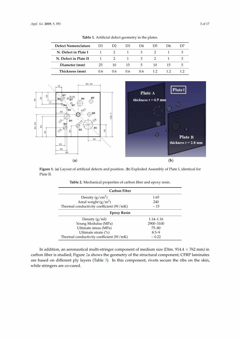
special bracket is conceived with specific geometric dimensions for Plexiglas wedge (as seen in Figure

4a), constructed in thermoplastic polymeric material PLA with Ultimaker2 3D printer. Figure 4b

show experimental setup employed on CFRP component in direct contact with aid of coupling gel,

since water stream method would give similar results.

(a) (b)

Figure 4. (a) CATIA assembly view of new PLA bracket tool and (b) experimental setup for ultrasonic

C-scan controls around simulated impact zone of aeronautical component.

Thermal pulsed acquisitions of multi-stringer part are successively performed and focused on

central impacted damage area to verify defect data correlation with UT controls.

Aeronautical component surface is positioned at a higher distance of 0.72 m from the four

halogen lamps than CFRP plates, due to necessary of inspection on a larger delamination zone around

the impact simulated cut with a fixed focal point of the camera. Figure 5 shows the thermographic

setup that is used for all tests described in the case of computed inspection.

Employing this set-up, pulsed thermography is executed on CFRP component, in the central

zone; five total tests are conducted, by selecting different heating times (Table 5).

All tests are performed in controlled ambient temperature between 21–25 °C for thermal analysis

on CFRP elements, monitored by humidity/temperature data logger PCE-HT110, without input in

the camera software.

Figure 4. (a) CATIA assembly view of new PLA bracket tool and (b) experimental setup for ultrasonicC-scan controls around simulated impact zone of aeronautical component.

The authors used the UT C-scan technique to provide a two-dimensional representation of defectsin a specific parallel plane below inspected surface and scans of ultrasonic data are synchronized withthe unidirectional movement of the probe itself, along the main scan line and this is possible by rigidlycoupling an encoder to the ultrasonic probe, moving along a sliding guide.

In previous works, appropriate UT tools are designed to allow stable coupling to GFRPcomponents [23] with ultrasonic inspections. In our case, ultrasonic probe must be maintainedin a steady orientation and contact conditions relative to inspected component [23] and for this goal,a special bracket is conceived with specific geometric dimensions for Plexiglas wedge (as seen inFigure 4a), constructed in thermoplastic polymeric material PLA with Ultimaker2 3D printer. Figure 4bshow experimental setup employed on CFRP component in direct contact with aid of coupling gel,since water stream method would give similar results.

Thermal pulsed acquisitions of multi-stringer part are successively performed and focused oncentral impacted damage area to verify defect data correlation with UT controls.

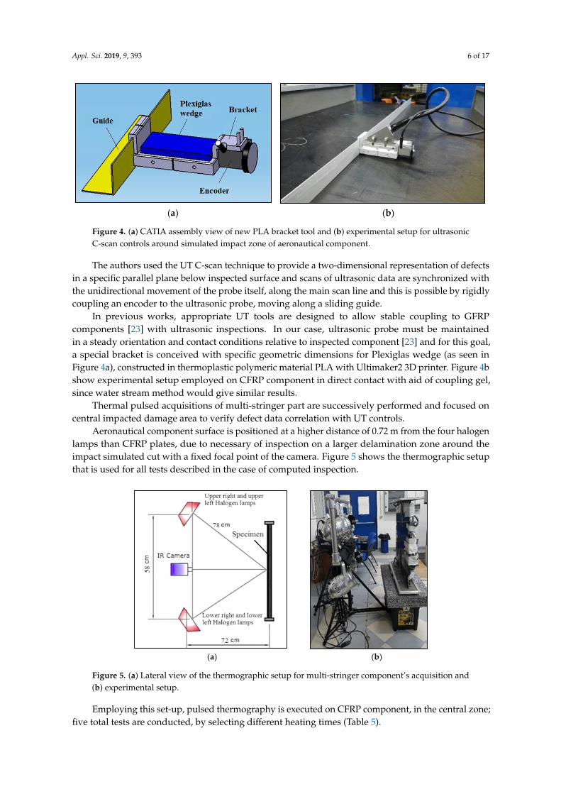
Aeronautical component surface is positioned at a higher distance of 0.72 m from the four halogenlamps than CFRP plates, due to necessary of inspection on a larger delamination zone around theimpact simulated cut with a fixed focal point of the camera. Figure 5 shows the thermographic setupthat is used for all tests described in the case of computed inspection.Appl. Sci. 2018, 8, x FOR PEER REVIEW 7 of 18

(a) (b)

Figure 5. (a) Lateral view of the thermographic setup for multi-stringer component’s acquisition and

(b) experimental setup.

Table 5. Scheduling tests for the multi-stringer component’s investigation

N°

Test

Frame Rate

[Hz]

Heating

Time [s]

Acquisition

Time [s]

Total

Frames 1 5 20 100 500

2 5 30 100 500

3 5 40 100 500

4 5 12 200 1000

5 5 15 200 1000

3. Data Processing and Image Elaboration Procedures

The thermal contrast is the chosen parameter for defect localization by means of pulsed

thermography; the surface temperature contrast is used to better investigate defect detectability and

offers a qualitative comparison between standard defect and real delamination. Automatic advanced

image-processing with preliminary algorithm is implemented in the MATLAB R2014b (The

MathWorks, Inc., Natick, MA, USA, 2014) environment, to upload the three-dimensional matrix of

thermal frames and to return selected thermal maps of specimen for various tests; local contrast is

determined, highlighting various heat accumulation sites obtained over time, intact zones, and

damaged areas [20] processed together with the absolute contrast parameter CA, defined by the

equation

𝑪𝑨(𝒕) = 𝑻𝑫𝒁 − 𝑻𝑰𝒁 (1)

Where the two terms TDZ and TIZ are the mean temperature in defect and intact zones during the

cooling phase. Contrast analysis has limitation due to the used set-up and the operator’s choice of

reference intact areas for the contrast computation, for which following applied examples show some

variability of results and correct definition of suitable intact reference zone for each selected defect is

time consuming, especially if implemented in automated analysis.

The authors suggest developing an algorithm with different approach, to possibly improve

defect and visibility defect shape on the base of absolute contrast approach. Preliminary study is

conducted to investigate defect by raw temperatures analysis in a chosen thermal frame; defect

characterization and automated contrast mapping with accurate methodology represent the main

purpose of paper.

In this work, temperature perturbations as function of variable time is not considered for

simplicity and a contrast enhance algorithm is proposed to map his values, as distributed completely

Figure 5. (a) Lateral view of the thermographic setup for multi-stringer component’s acquisition and(b) experimental setup.

Employing this set-up, pulsed thermography is executed on CFRP component, in the central zone;five total tests are conducted, by selecting different heating times (Table 5).

Appl. Sci. 2019, 9, 393 7 of 17

Table 5. Scheduling tests for the multi-stringer component’s investigation.

N◦ Test Frame Rate [Hz] Heating Time [s] Acquisition Time [s] Total Frames

1 5 20 100 5002 5 30 100 5003 5 40 100 5004 5 12 200 10005 5 15 200 1000

All tests are performed in controlled ambient temperature between 21–25 ◦C for thermal analysison CFRP elements, monitored by humidity/temperature data logger PCE-HT110, without input in thecamera software.

3. Data Processing and Image Elaboration Procedures

The thermal contrast is the chosen parameter for defect localization by means of pulsedthermography; the surface temperature contrast is used to better investigate defect detectability andoffers a qualitative comparison between standard defect and real delamination. Automatic advancedimage-processing with preliminary algorithm is implemented in the MATLAB R2014b (The MathWorks,Inc., Natick, MA, USA, 2014) environment, to upload the three-dimensional matrix of thermal framesand to return selected thermal maps of specimen for various tests; local contrast is determined,highlighting various heat accumulation sites obtained over time, intact zones, and damaged areas [20]processed together with the absolute contrast parameter CA, defined by the equation

CA(t) = TDZ − TIZ (1)

where the two terms TDZ and TIZ are the mean temperature in defect and intact zones during thecooling phase. Contrast analysis has limitation due to the used set-up and the operator’s choice ofreference intact areas for the contrast computation, for which following applied examples show somevariability of results and correct definition of suitable intact reference zone for each selected defect istime consuming, especially if implemented in automated analysis.

The authors suggest developing an algorithm with different approach, to possibly improve defectand visibility defect shape on the base of absolute contrast approach. Preliminary study is conductedto investigate defect by raw temperatures analysis in a chosen thermal frame; defect characterizationand automated contrast mapping with accurate methodology represent the main purpose of paper.

In this work, temperature perturbations as function of variable time is not considered for simplicityand a contrast enhance algorithm is proposed to map his values, as distributed completely on wholeinspected specimen. This enhanced thermal contrast algorithm automates the simultaneous detectionand mapping of contrast as optimized to identify defect boundaries according only to spatial variationsin neighboring of each [i, j]th calculation point in the whole frame; in other words, the local contrastis automatically determined by calculating in the surroundings of a highest temperature spot inpre-defined areas the temperature variation ∆T. For a general location [i, j] on the thermal image,the new contrast parameter C is defined through the formula

C(i,j) = ∆T(i, j) =∣∣∣TD(i,j)

− TIZ(i,j)

∣∣∣ (2)

where, for each pixel of the thermographic image, the implemented MATLAB algorithm reworks thedifferences of the two mean temperatures TD(i,j) of the presumed defect in [i, j]th calculation point andTIZ(i,j) temperature, calculated as mean value in a reference rectangular zone around [i, j]th calculationpoint. The new algorithm is based on basic principle that reference temperatures evaluated around theinspected spot tends to maximize different values when trepassing the defect border, leading to localcontrast variations to be displayed, clearly distinguishing defect shape and boundaries.

Appl. Sci. 2019, 9, 393 8 of 17

The algorithm processes temperatures in iterative manner over the whole thermal map,without choosing an intact reference zone. This elaboration was inspired by DIC technique, where thecorrelation between the pixels does not occur in a temporal way, but punctual way, highlighting themaximum contrast reached in the proximity of defect border.

3.1. Reference Absolute Contrast

Even when undamaged zone definition is straightforward, considerable variations of results areobserved with different location choice of reference zone and with different dimension of the identifieddamaged area.

The source distribution image (SDI) was developed for selecting free-defects portions of specimenthat receives the same thermal flow of the corresponding inspected spot [24].

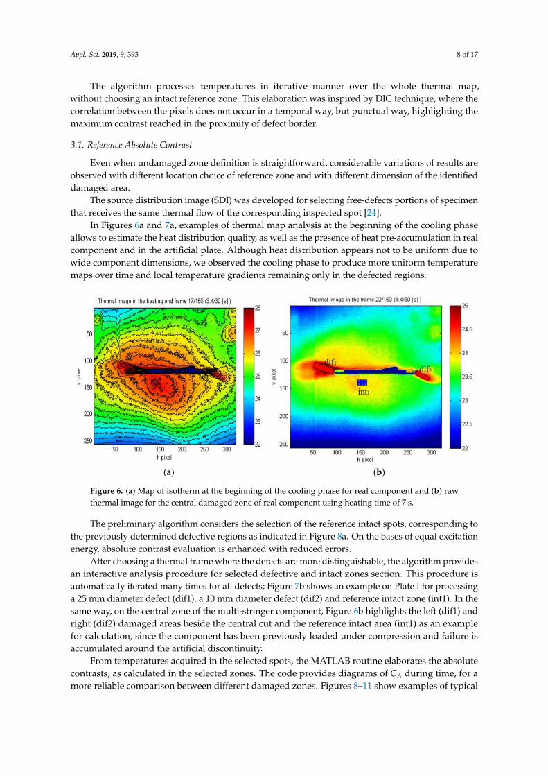
In Figures 6a and 7a, examples of thermal map analysis at the beginning of the cooling phaseallows to estimate the heat distribution quality, as well as the presence of heat pre-accumulation in realcomponent and in the artificial plate. Although heat distribution appears not to be uniform due towide component dimensions, we observed the cooling phase to produce more uniform temperaturemaps over time and local temperature gradients remaining only in the defected regions.


on whole inspected specimen. This enhanced thermal contrast algorithm automates the simultaneous

detection and mapping of contrast as optimized to identify defect boundaries according only to

spatial variations in neighboring of each [i, j]th calculation point in the whole frame; in other words,

the local contrast is automatically determined by calculating in the surroundings of a highest

temperature spot in pre-defined areas the temperature variation ΔT. For a general location [i, j] on

the thermal image, the new contrast parameter C is defined through the formula

𝑪(𝒊,𝒋) = ∆𝑻(𝒊,𝒋) = |𝑻𝑫(𝒊,𝒋) − 𝑻𝑰𝒁(𝒊,𝒋)

| (2)

where, for each pixel of the thermographic image, the implemented MATLAB algorithm reworks the

differences of the two mean temperatures TD(i,j) of the presumed defect in [i, j]th calculation point and

TIZ(i,j) temperature, calculated as mean value in a reference rectangular zone around [i, j]th calculation

point. The new algorithm is based on basic principle that reference temperatures evaluated around

the inspected spot tends to maximize different values when trepassing the defect border, leading to

local contrast variations to be displayed, clearly distinguishing defect shape and boundaries.

The algorithm processes temperatures in iterative manner over the whole thermal map, without

choosing an intact reference zone. This elaboration was inspired by DIC technique, where the

correlation between the pixels does not occur in a temporal way, but punctual way, highlighting the

maximum contrast reached in the proximity of defect border.

3.1. Reference Absolute Contrast

Even when undamaged zone definition is straightforward, considerable variations of results are

observed with different location choice of reference zone and with different dimension of the

identified damaged area.

The source distribution image (SDI) was developed for selecting free-defects portions of

specimen that receives the same thermal flow of the corresponding inspected spot [24].

(a) (b)

Figure 6. (a) Map of isotherm at the beginning of the cooling phase for real component and (b) raw

thermal image for the central damaged zone of real component using heating time of 7 s.

In Figures 6a and 7a, examples of thermal map analysis at the beginning of the cooling phase

allows to estimate the heat distribution quality, as well as the presence of heat pre-accumulation in

real component and in the artificial plate. Although heat distribution appears not to be uniform due

to wide component dimensions, we observed the cooling phase to produce more uniform

temperature maps over time and local temperature gradients remaining only in the defected regions.

The preliminary algorithm considers the selection of the reference intact spots, corresponding to

the previously determined defective regions as indicated in Figure 8a. On the bases of equal excitation

energy, absolute contrast evaluation is enhanced with reduced errors.

Figure 6. (a) Map of isotherm at the beginning of the cooling phase for real component and (b) rawthermal image for the central damaged zone of real component using heating time of 7 s.

The preliminary algorithm considers the selection of the reference intact spots, corresponding tothe previously determined defective regions as indicated in Figure 8a. On the bases of equal excitationenergy, absolute contrast evaluation is enhanced with reduced errors.

After choosing a thermal frame where the defects are more distinguishable, the algorithm providesan interactive analysis procedure for selected defective and intact zones section. This procedure isautomatically iterated many times for all defects; Figure 7b shows an example on Plate I for processinga 25 mm diameter defect (dif1), a 10 mm diameter defect (dif2) and reference intact zone (int1). In thesame way, on the central zone of the multi-stringer component, Figure 6b highlights the left (dif1) andright (dif2) damaged areas beside the central cut and the reference intact area (int1) as an examplefor calculation, since the component has been previously loaded under compression and failure isaccumulated around the artificial discontinuity.

From temperatures acquired in the selected spots, the MATLAB routine elaborates the absolutecontrasts, as calculated in the selected zones. The code provides diagrams of CA during time, for amore reliable comparison between different damaged zones. Figures 8–11 show examples of typical

Appl. Sci. 2019, 9, 393 9 of 17

thermal profiles of intact zones and defective areas and the relative Absolute contrast behavior; in bothcases, CA gives values from 0.9◦C up to 4◦C, indicating the defect intensity.


After choosing a thermal frame where the defects are more distinguishable, the algorithm

provides an interactive analysis procedure for selected defective and intact zones section. This

procedure is automatically iterated many times for all defects; Figure 7b shows an example on Plate

I for processing a 25 mm diameter defect (dif1), a 10 mm diameter defect (dif2) and reference intact

zone (int1). In the same way, on the central zone of the multi-stringer component, Figure 6b highlights

the left (dif1) and right (dif2) damaged areas beside the central cut and the reference intact area (int1)

as an example for calculation, since the component has been previously loaded under compression

and failure is accumulated around the artificial discontinuity.

(a) (b)

Figure 7. (a) Map of isotherms at the beginning of the cooling phase for artificial Plate I and (b) defect

presence example on raw thermal image, using heating time of 20 s.

From temperatures acquired in the selected spots, the MATLAB routine elaborates the absolute

contrasts, as calculated in the selected zones. The code provides diagrams of CA during time, for a

more reliable comparison between different damaged zones. Figures 8,9,10, and 11 show examples

of typical thermal profiles of intact zones and defective areas and the relative Absolute contrast

behavior; in both cases, CA gives values from 0.9°C up to 4°C, indicating the defect intensity.

(a) (b)

Figure 8. (a) Thermal profiles and (b) absolute contrast example for defect-1 (Ø 25 mm) and intact

area in Plate I, using heating time of 20 s.

Figure 7. (a) Map of isotherms at the beginning of the cooling phase for artificial Plate I and (b) defectpresence example on raw thermal image, using heating time of 20 s.


After choosing a thermal frame where the defects are more distinguishable, the algorithm

provides an interactive analysis procedure for selected defective and intact zones section. This

procedure is automatically iterated many times for all defects; Figure 7b shows an example on Plate

I for processing a 25 mm diameter defect (dif1), a 10 mm diameter defect (dif2) and reference intact

zone (int1). In the same way, on the central zone of the multi-stringer component, Figure 6b highlights

the left (dif1) and right (dif2) damaged areas beside the central cut and the reference intact area (int1)

as an example for calculation, since the component has been previously loaded under compression

and failure is accumulated around the artificial discontinuity.

(a) (b)

Figure 7. (a) Map of isotherms at the beginning of the cooling phase for artificial Plate I and (b) defect

presence example on raw thermal image, using heating time of 20 s.

From temperatures acquired in the selected spots, the MATLAB routine elaborates the absolute

contrasts, as calculated in the selected zones. The code provides diagrams of CA during time, for a

more reliable comparison between different damaged zones. Figures 8,9,10, and 11 show examples

of typical thermal profiles of intact zones and defective areas and the relative Absolute contrast

behavior; in both cases, CA gives values from 0.9°C up to 4°C, indicating the defect intensity.

(a) (b)



Figure 8. (a) Thermal profiles and (b) absolute contrast example for defect-1 (Ø 25 mm) and intact areain Plate I, using heating time of 20 s.


(a) (b)



(a) (b)

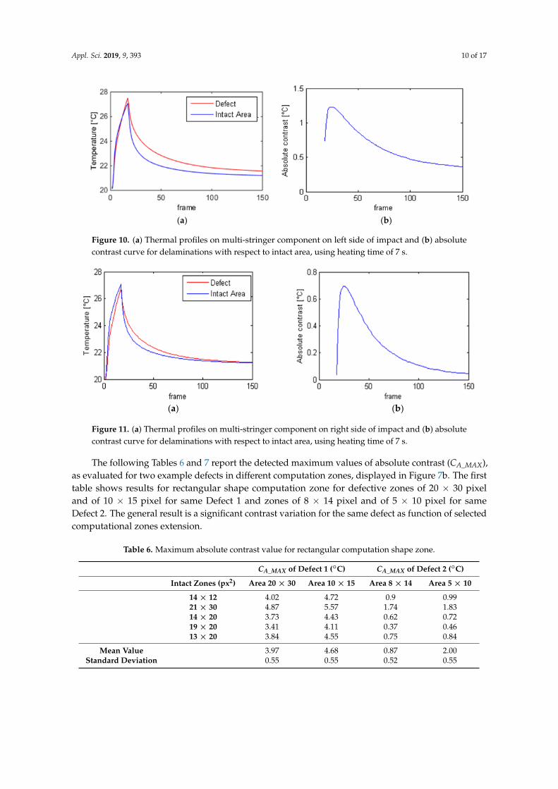
Figure 10. (a) Thermal profiles on multi-stringer component on left side of impact and (b) absolute

contrast curve for delaminations with respect to intact area, using heating time of 7 s.

(a) (b)

Figure 11. (a) Thermal profiles on multi-stringer component on right side of impact and (b) absolute


The following Tables 6 and 7 report the detected maximum values of absolute contrast (CA_MAX),

as evaluated for two example defects in different computation zones, displayed in Figure 7b. The first

table shows results for rectangular shape computation zone for defective zones of 20 × 30 pixel and

of 10 × 15 pixel for same Defect 1 and zones of 8 × 14 pixel and of 5 × 10 pixel for same Defect 2. The

Figure 9. (a) Thermal profiles and (b) absolute contrast example for defect-2 (Ø 10 mm) and intact areain Plate I, using heating time of 20 s.

Appl. Sci. 2019, 9, 393 10 of 17


(a) (b)



(a) (b)



(a) (b)







Figure 10. (a) Thermal profiles on multi-stringer component on left side of impact and (b) absolutecontrast curve for delaminations with respect to intact area, using heating time of 7 s.


(a) (b)



(a) (b)



(a) (b)







Figure 11. (a) Thermal profiles on multi-stringer component on right side of impact and (b) absolutecontrast curve for delaminations with respect to intact area, using heating time of 7 s.

The following Tables 6 and 7 report the detected maximum values of absolute contrast (CA_MAX),as evaluated for two example defects in different computation zones, displayed in Figure 7b. The firsttable shows results for rectangular shape computation zone for defective zones of 20 × 30 pixeland of 10 × 15 pixel for same Defect 1 and zones of 8 × 14 pixel and of 5 × 10 pixel for sameDefect 2. The general result is a significant contrast variation for the same defect as function of selectedcomputational zones extension.

Table 6. Maximum absolute contrast value for rectangular computation shape zone.

CA_MAX of Defect 1 (◦C) CA_MAX of Defect 2 (◦C)

Intact Zones (px2) Area 20 × 30 Area 10 × 15 Area 8 × 14 Area 5 × 10

14 × 12 4.02 4.72 0.9 0.9921 × 30 4.87 5.57 1.74 1.8314 × 20 3.73 4.43 0.62 0.7219 × 20 3.41 4.11 0.37 0.4613 × 20 3.84 4.55 0.75 0.84

Mean Value 3.97 4.68 0.87 2.00Standard Deviation 0.55 0.55 0.52 0.55

Appl. Sci. 2019, 9, 393 11 of 17

Table 7. Maximum absolute contrast value for rectangular and circular computation shape zone.

CA_MAX (◦C)

Rectangular Area (px*px) Circular Area (Ø px)

Intact Zone Size Def. 120 × 30

Def. 28 × 14

Intact ZoneSize

Def. 1Ø 33

Def. 2Ø 9

14 × 12 4.02 0.9 14 1.27 1.8121 × 30 4.87 1.74 30 0.91 1.4914 × 20 3.73 0.62 20 1.11 1.6819 × 20 3.41 0.37 16 2.38 2.9013 × 20 3.84 0.75 18 1.69 2.12

Mean Value 3.97 0.87 1.47 2.00Standard Deviation 0.55 0.52 0.58 0.55

The second Table compares results for rectangular and circular shape zones (diameter Ø 33 pixelfor Defect 1 and diameter Ø 9 pixel for Defect 2), as seen in Figure 12, showing higher contrast valuesin the case of rectangular shape with respect to circular shapes for defect 1 in any zone size and highercontrast values in the case of circular shape zones for Defect 2. These Tables illustrate the variationcontrast results with the operator choice of both shapes and size for reference and damaged areas.Appl. Sci. 2018, 8, x FOR PEER REVIEW 12 of 18

Figure 12. Raw thermal image of Plate I with circular reference zones and defect’s relative Absolute

contrast examples.

3.2. Custom Mapping Optimization in Terms of Thermal Contrast Measurements

The determination of the thermal contrast has the limitation to be performed at the local level

and undergoes preliminary costly choices of specific thermal frames and zones to be investigated.

When the heat quantity deposited by the external source is not uniform and the computation zones

have slightly different cooling temperatures and gradients, some defects can be misjudged as

identical. In any case, is necessary to analyze a single defect at a time: therefore, it was necessary a

new method to be implemented on MATLAB and take in account such limitation and improve the

processing technique to enhance the inspection defects in terms of accuracy and reduced time.

The new contrast algorithm allows direct defect mapping on the case of the value of contrasts,

as distributed on inspected specimen. In this way, the method automates the determination and

mapping simultaneously of the local contrast, to identify defect boundaries onto the analyzed

component. In other words, the local contrast is automatically determined, investigating every zone

with highest temperature in pre-defined areas.

For each pixel of the thermographic image, new MATLAB procedures rework the variation of

temperatures determined in a two-dimensional array of pixels in the proximity of the calculation

point. This algorithm is based on the principle for which temperatures computed around the chosen

inspected spot tend to reach similar values when location corresponds to defect border, leading to

contrast values being displayed with zero values on contrast maps, clearly distinguishing the

damaged zones and defect shape. Figure 13 shows a comparison between original thermal map

(Figure 13a) and the proposed contrast image (Figure 13b) of CFRP Plate I on Side B (defects’ depth

of 2.8 mm) obtained after 11.6 cooling seconds after heating pulse of 20 s.

Figure 12. Raw thermal image of Plate I with circular reference zones and defect’s relative Absolutecontrast examples.

In the Tables, we can notice the intact zone’s choice significantly influences the analyticaldetermination of the thermal contrast curve, used to characterize the defect intensity. From theprevious images, sometimes heat is not uniform on the specimen surface and the choice of intact areasis a determining factor in the contrast computation.

Simple circular shape is chosen because optimal for artificial circular defects, instead rectangularshape is considered firstly because very different with respect to circular shape and capable to detectdelaminations in structural squared real elements.

Appl. Sci. 2019, 9, 393 12 of 17

3.2. Custom Mapping Optimization in Terms of Thermal Contrast Measurements

The determination of the thermal contrast has the limitation to be performed at the local leveland undergoes preliminary costly choices of specific thermal frames and zones to be investigated.When the heat quantity deposited by the external source is not uniform and the computation zoneshave slightly different cooling temperatures and gradients, some defects can be misjudged as identical.In any case, is necessary to analyze a single defect at a time: therefore, it was necessary a new methodto be implemented on MATLAB and take in account such limitation and improve the processingtechnique to enhance the inspection defects in terms of accuracy and reduced time.

The new contrast algorithm allows direct defect mapping on the case of the value of contrasts,as distributed on inspected specimen. In this way, the method automates the determination andmapping simultaneously of the local contrast, to identify defect boundaries onto the analyzedcomponent. In other words, the local contrast is automatically determined, investigating everyzone with highest temperature in pre-defined areas.

For each pixel of the thermographic image, new MATLAB procedures rework the variation oftemperatures determined in a two-dimensional array of pixels in the proximity of the calculationpoint. This algorithm is based on the principle for which temperatures computed around the choseninspected spot tend to reach similar values when location corresponds to defect border, leading tocontrast values being displayed with zero values on contrast maps, clearly distinguishing the damagedzones and defect shape. Figure 13 shows a comparison between original thermal map (Figure 13a) andthe proposed contrast image (Figure 13b) of CFRP Plate I on Side B (defects’ depth of 2.8 mm) obtainedafter 11.6 cooling seconds after heating pulse of 20 s.Appl. Sci. 2018, 8, x FOR PEER REVIEW 13 of 18

(a) (b)

Figure 13. (a) Example of comparison between raw thermal map and (b) contrast map of CFRP Plate

I/Side B.

Despite the heating not ideal, the contrasts map allows identification even the smallest defects

of 5 mm diameter in a single specimen map (top left). The proposed contrast allows better evaluation

of internal defects and is physically explained by the fact the thermal properties of defects are

different from those of the surrounding material.

Contrast mapping has been optimized in order to highlight the most reliable boundary for

defects of various types in carbon fiber plates, significantly reducing the noise effects and erroneous

defective indications.

The greater depth of defects in the Plate I/Side A (4.9 mm of depth, in Figure 14a) causes

difficulty of plate inspection and therefore we use longest heating times (Table 4). In the contrast map

of Plate II/Side A (Figure 15b), four small defects of 5 mm diameter are clearly distinguished. Since,

higher heating times do not allow smaller and deep defects detection; therefore, higher defect depth

remain the main inspection limit and it was not possible to identify defects with less than 15 mm

diameter (denominated D2, D4, D5, and D7 in Table 1) in figure 14b, consequently the method allows

to better distinguish all defects, but the physical limit of higher depth remains and small defects are

still not visible. From CFRP Plate II acquisitions, the heating time of 15 s allows us to detect more

clearly the greatest number of defects.

(a) (b)

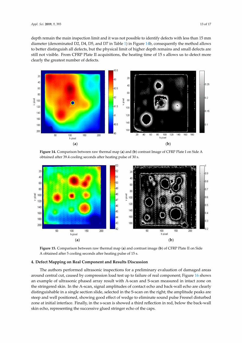
Figure 14. Comparison between raw thermal map (a) and (b) contrast Image of CFRP Plate I on Side

A obtained after 39.4 cooling seconds after heating pulse of 30 s.

Figure 13. (a) Example of comparison between raw thermal map and (b) contrast map of CFRP PlateI/Side B.

Despite the heating not ideal, the contrasts map allows identification even the smallest defects of5 mm diameter in a single specimen map (top left). The proposed contrast allows better evaluation ofinternal defects and is physically explained by the fact the thermal properties of defects are differentfrom those of the surrounding material.

Contrast mapping has been optimized in order to highlight the most reliable boundary fordefects of various types in carbon fiber plates, significantly reducing the noise effects and erroneousdefective indications.

The greater depth of defects in the Plate I/Side A (4.9 mm of depth, in Figure 14a) causesdifficulty of plate inspection and therefore we use longest heating times (Table 4). In the contrastmap of Plate II/Side A (Figure 15b), four small defects of 5 mm diameter are clearly distinguished.Since, higher heating times do not allow smaller and deep defects detection; therefore, higher defect

Appl. Sci. 2019, 9, 393 13 of 17

depth remain the main inspection limit and it was not possible to identify defects with less than 15 mmdiameter (denominated D2, D4, D5, and D7 in Table 1) in Figure 14b, consequently the method allowsto better distinguish all defects, but the physical limit of higher depth remains and small defects arestill not visible. From CFRP Plate II acquisitions, the heating time of 15 s allows us to detect moreclearly the greatest number of defects.


(a) (b)

Figure 13. (a) Example of comparison between raw thermal map and (b) contrast map of CFRP Plate

I/Side B.

Despite the heating not ideal, the contrasts map allows identification even the smallest defects

of 5 mm diameter in a single specimen map (top left). The proposed contrast allows better evaluation

of internal defects and is physically explained by the fact the thermal properties of defects are

different from those of the surrounding material.

Contrast mapping has been optimized in order to highlight the most reliable boundary for

defects of various types in carbon fiber plates, significantly reducing the noise effects and erroneous

defective indications.

The greater depth of defects in the Plate I/Side A (4.9 mm of depth, in Figure 14a) causes

difficulty of plate inspection and therefore we use longest heating times (Table 4). In the contrast map

of Plate II/Side A (Figure 15b), four small defects of 5 mm diameter are clearly distinguished. Since,

higher heating times do not allow smaller and deep defects detection; therefore, higher defect depth

remain the main inspection limit and it was not possible to identify defects with less than 15 mm

diameter (denominated D2, D4, D5, and D7 in Table 1) in figure 14b, consequently the method allows

to better distinguish all defects, but the physical limit of higher depth remains and small defects are

still not visible. From CFRP Plate II acquisitions, the heating time of 15 s allows us to detect more

clearly the greatest number of defects.

(a) (b)

Figure 14. Comparison between raw thermal map (a) and (b) contrast Image of CFRP Plate I on Side

A obtained after 39.4 cooling seconds after heating pulse of 30 s.

Figure 14. Comparison between raw thermal map (a) and (b) contrast Image of CFRP Plate I on Side Aobtained after 39.4 cooling seconds after heating pulse of 30 s.


(a) (b)

Figure 15. Comparison between raw thermal map (a) and contrast image (b) of CFRP Plate II on Side

A obtained after 5 cooling seconds after heating pulse of 15 s.

4. Defect Mapping on Real Component and Results Discussion

The authors performed ultrasonic inspections for a preliminary evaluation of damaged areas

around central cut, caused by compression load test up to failure of real component; Figure 16 shows

an example of ultrasonic phased array result with A-scan and S-scan measured in intact zone on the

stringered skin. In the A-scan, signal amplitudes of contact echo and back-wall echo are clearly

distinguishable in a single section slide, selected in the S-scan on the right; the amplitude peaks are

steep and well positioned, showing good effect of wedge to eliminate sound pulse Fresnel disturbed

zone at initial interface. Finally, in the s-scan is showed a third reflection in red, below the back-wall

skin echo, representing the successive glued stringer echo of the caps.

For defect presence and size evaluation, a whole C-scan mapping of the damaged area is

conducted in the functional direction along the simulated impact, where in Figure 17 are clearly

highlighted the delamination distribution and their boundaries. The C-scan depth limits of UT

inspections are chosen between 0.79 and 5.41 mm to analyze only the internal skin and not the

skin/stringer interface below it.

Figure 16. A-scan (left) and S-scan (right) of non-damaged zone around impact simulation cut.

Figure 15. Comparison between raw thermal map (a) and contrast image (b) of CFRP Plate II on SideA obtained after 5 cooling seconds after heating pulse of 15 s.


The authors performed ultrasonic inspections for a preliminary evaluation of damaged areasaround central cut, caused by compression load test up to failure of real component; Figure 16 showsan example of ultrasonic phased array result with A-scan and S-scan measured in intact zone onthe stringered skin. In the A-scan, signal amplitudes of contact echo and back-wall echo are clearlydistinguishable in a single section slide, selected in the S-scan on the right; the amplitude peaks aresteep and well positioned, showing good effect of wedge to eliminate sound pulse Fresnel disturbedzone at initial interface. Finally, in the s-scan is showed a third reflection in red, below the back-wallskin echo, representing the successive glued stringer echo of the caps.

Appl. Sci. 2019, 9, 393 14 of 17


(a) (b)

Figure 15. Comparison between raw thermal map (a) and contrast image (b) of CFRP Plate II on Side

A obtained after 5 cooling seconds after heating pulse of 15 s.


The authors performed ultrasonic inspections for a preliminary evaluation of damaged areas

around central cut, caused by compression load test up to failure of real component; Figure 16 shows

an example of ultrasonic phased array result with A-scan and S-scan measured in intact zone on the

stringered skin. In the A-scan, signal amplitudes of contact echo and back-wall echo are clearly

distinguishable in a single section slide, selected in the S-scan on the right; the amplitude peaks are

steep and well positioned, showing good effect of wedge to eliminate sound pulse Fresnel disturbed

zone at initial interface. Finally, in the s-scan is showed a third reflection in red, below the back-wall

skin echo, representing the successive glued stringer echo of the caps.

For defect presence and size evaluation, a whole C-scan mapping of the damaged area is

conducted in the functional direction along the simulated impact, where in Figure 17 are clearly

highlighted the delamination distribution and their boundaries. The C-scan depth limits of UT

inspections are chosen between 0.79 and 5.41 mm to analyze only the internal skin and not the

skin/stringer interface below it.

Figure 16. A-scan (left) and S-scan (right) of non-damaged zone around impact simulation cut. Figure 16. A-scan (left) and S-scan (right) of non-damaged zone around impact simulation cut.

For defect presence and size evaluation, a whole C-scan mapping of the damaged area isconducted in the functional direction along the simulated impact, where in Figure 17 are clearlyhighlighted the delamination distribution and their boundaries. The C-scan depth limits of UTinspections are chosen between 0.79 and 5.41 mm to analyze only the internal skin and not theskin/stringer interface below it.


Figure 17. C-scan inspection over the multi-stringer component’s surface on damaged zone along the

artificial cut and an example of A-scan and S-scan on right side delamination.

In Figure 18, two ultrasonic local scans of damaged zone are representative of the widespread

asymmetrical delaminations around the cut extremities, due to compression load testing. In the

figures’ s-scans, a linear 0° S-scan direction normal to inspected skin surface is presented with a 38

mm horizontal axis width, corresponding to probe array length; evident multiple delamination

echoes between several composite layers are displayed in both figures in the red zones of s-scans

below the surface at depth in the range 2–3 mm, whose extension in progressively expanding more

than 30 mm in width in different way at right- or left-side damage level is particularly elevate and

back-wall/stringer signal disappear below the delaminated zone.

(a) (b)

Figure 18. A-scan and S-scan of two damaged zones on the left side (a) and the right side (b) of impact

simulation cut of multi-stringer component.

These UT results are compared with the thermographic analysis, using the specific setup and

the experimental tests previously described. Thermal acquisitions are described in Table 5, with

heating time of 3 s and 10 s, and data are processed for contrast mapping, as shown in Figure 19a and

19b respectively. Thermographic inspections result shows delaminations clearly visible, but in this

case, the local contrast map seems to slightly underestimate the defect extension with respect to UT

C-scan results. This could be due to better calibration needs for the used algorithm on larger specimen

sizes and geometry of target surface to inspect; in addition, the contrast map presents some

differences than UT results as being referred primarily more realistic defect features in case of large

delaminations. The authors, in fact, assume that the outer edges of the delaminations are extremely

thin and in contact with each other, giving rise to occasional thermal continuity also in the damage

area and this explains the difference from the thermographic point of view. For artificial defects this

problem is absent and the enhanced contrast mapping procedure is optimized for the latter case.

The damage dimensions on left side of artificial impact simulation defect are estimated around

an area of 112.5 × 50 mm with the UT C-scan map; from raw temperature maps in Figure 6a and

converting dimensions from pixels to millimeters, the delamination size is roughly in an area of 78 ×

38.5 mm and in alternative way equal to an area of 65.26 × 20 mm as measured from Figure 20,

Figure 17. C-scan inspection over the multi-stringer component’s surface on damaged zone along theartificial cut and an example of A-scan and S-scan on right side delamination.

In Figure 18, two ultrasonic local scans of damaged zone are representative of the widespreadasymmetrical delaminations around the cut extremities, due to compression load testing. In thefigures’ s-scans, a linear 0◦ S-scan direction normal to inspected skin surface is presented with a 38 mmhorizontal axis width, corresponding to probe array length; evident multiple delamination echoesbetween several composite layers are displayed in both figures in the red zones of s-scans below thesurface at depth in the range 2–3 mm, whose extension in progressively expanding more than 30 mm inwidth in different way at right- or left-side damage level is particularly elevate and back-wall/stringersignal disappear below the delaminated zone.

These UT results are compared with the thermographic analysis, using the specific setup andthe experimental tests previously described. Thermal acquisitions are described in Table 5, withheating time of 3 s and 10 s, and data are processed for contrast mapping, as shown in Figure 19a,brespectively. Thermographic inspections result shows delaminations clearly visible, but in this case,the local contrast map seems to slightly underestimate the defect extension with respect to UT C-scanresults. This could be due to better calibration needs for the used algorithm on larger specimen sizes

Appl. Sci. 2019, 9, 393 15 of 17

and geometry of target surface to inspect; in addition, the contrast map presents some differences thanUT results as being referred primarily more realistic defect features in case of large delaminations.The authors, in fact, assume that the outer edges of the delaminations are extremely thin and in contactwith each other, giving rise to occasional thermal continuity also in the damage area and this explainsthe difference from the thermographic point of view. For artificial defects this problem is absent andthe enhanced contrast mapping procedure is optimized for the latter case.


Figure 17. C-scan inspection over the multi-stringer component’s surface on damaged zone along the

artificial cut and an example of A-scan and S-scan on right side delamination.

In Figure 18, two ultrasonic local scans of damaged zone are representative of the widespread

asymmetrical delaminations around the cut extremities, due to compression load testing. In the

figures’ s-scans, a linear 0° S-scan direction normal to inspected skin surface is presented with a 38

mm horizontal axis width, corresponding to probe array length; evident multiple delamination

echoes between several composite layers are displayed in both figures in the red zones of s-scans

below the surface at depth in the range 2–3 mm, whose extension in progressively expanding more

than 30 mm in width in different way at right- or left-side damage level is particularly elevate and

back-wall/stringer signal disappear below the delaminated zone.

(a) (b)

Figure 18. A-scan and S-scan of two damaged zones on the left side (a) and the right side (b) of impact

simulation cut of multi-stringer component.

These UT results are compared with the thermographic analysis, using the specific setup and

the experimental tests previously described. Thermal acquisitions are described in Table 5, with

heating time of 3 s and 10 s, and data are processed for contrast mapping, as shown in Figure 19a and

19b respectively. Thermographic inspections result shows delaminations clearly visible, but in this

case, the local contrast map seems to slightly underestimate the defect extension with respect to UT

C-scan results. This could be due to better calibration needs for the used algorithm on larger specimen

sizes and geometry of target surface to inspect; in addition, the contrast map presents some

differences than UT results as being referred primarily more realistic defect features in case of large

delaminations. The authors, in fact, assume that the outer edges of the delaminations are extremely

thin and in contact with each other, giving rise to occasional thermal continuity also in the damage

area and this explains the difference from the thermographic point of view. For artificial defects this

problem is absent and the enhanced contrast mapping procedure is optimized for the latter case.

The damage dimensions on left side of artificial impact simulation defect are estimated around

an area of 112.5 × 50 mm with the UT C-scan map; from raw temperature maps in Figure 6a and

converting dimensions from pixels to millimeters, the delamination size is roughly in an area of 78 ×

38.5 mm and in alternative way equal to an area of 65.26 × 20 mm as measured from Figure 20,

Figure 18. A-scan and S-scan of two damaged zones on the left side (a) and the right side (b) of impactsimulation cut of multi-stringer component.


achieved with the contrast elaboration map; in both cases, it seems the internal delamination is less

extended and the UT inspections may overestimate the defect size. Furthermore, the new image

processing method, based on a correlation between local temperatures, is observed to present

disturbances when computed on the edges of the observed surface (the impact notch in the case of

real component) due to the thermal gradients between the component and the environment around

it, since the elaboration windows in a given point to be inspected will interfere with temperatures

outside the inspected part.

Real delamination begins at the edges of the notch, which does not appear in real scale in the

thermal map or contrast map due to the nature of the defect itself. Moreover, cause to larger size of

the investigated component, the thermal resolution displayed in Figure 20 is much lower than

resolution adopted for Plate I and Plate II specimens, giving rise to some differences originated by

the contrast algorithm determination.

(a) (b)

Figure 19. Contrast map of multi-stringer component using heating pulse of 3 s (a) and 10 s (b).

Figure 20. Contrast map of multi-stringer component using heating pulse of 7 s.

Future works may employ this new computation procedure on other NDT thermographic

techniques, as examples the lock-in method or PPT, on different defect type, in order to certify the

benefits of new contrast mapping.


The damage dimensions on left side of artificial impact simulation defect are estimated around anarea of 112.5 × 50 mm with the UT C-scan map; from raw temperature maps in Figure 6a and convertingdimensions from pixels to millimeters, the delamination size is roughly in an area of 78 × 38.5 mmand in alternative way equal to an area of 65.26 × 20 mm as measured from Figure 20, achievedwith the contrast elaboration map; in both cases, it seems the internal delamination is less extendedand the UT inspections may overestimate the defect size. Furthermore, the new image processingmethod, based on a correlation between local temperatures, is observed to present disturbances whencomputed on the edges of the observed surface (the impact notch in the case of real component) due tothe thermal gradients between the component and the environment around it, since the elaborationwindows in a given point to be inspected will interfere with temperatures outside the inspected part.

Appl. Sci. 2019, 9, 393 16 of 17


achieved with the contrast elaboration map; in both cases, it seems the internal delamination is less

extended and the UT inspections may overestimate the defect size. Furthermore, the new image

processing method, based on a correlation between local temperatures, is observed to present

disturbances when computed on the edges of the observed surface (the impact notch in the case of

real component) due to the thermal gradients between the component and the environment around

it, since the elaboration windows in a given point to be inspected will interfere with temperatures

outside the inspected part.

Real delamination begins at the edges of the notch, which does not appear in real scale in the

thermal map or contrast map due to the nature of the defect itself. Moreover, cause to larger size of

the investigated component, the thermal resolution displayed in Figure 20 is much lower than

resolution adopted for Plate I and Plate II specimens, giving rise to some differences originated by

the contrast algorithm determination.

(a) (b)



Future works may employ this new computation procedure on other NDT thermographic

techniques, as examples the lock-in method or PPT, on different defect type, in order to certify the

benefits of new contrast mapping.


Real delamination begins at the edges of the notch, which does not appear in real scale in thethermal map or contrast map due to the nature of the defect itself. Moreover, cause to larger size of theinvestigated component, the thermal resolution displayed in Figure 20 is much lower than resolutionadopted for Plate I and Plate II specimens, giving rise to some differences originated by the contrastalgorithm determination.

Future works may employ this new computation procedure on other NDT thermographictechniques, as examples the lock-in method or PPT, on different defect type, in order to certifythe benefits of new contrast mapping.

5. Conclusions

The contrast maps allow highlighting all the defects displayed in the corresponding thermal maps;the larger defects’ diameters are more noticeable than others, either on Side A or Side B of specimens.The depth at which the defects are located determines the thermographic visibility of the smaller onesand obviously, the defects observed are more easily identifiable and are greater in number if using thecontrast in elaborated maps than those detected in classic way.

The inspection on real multi-stringer CFRP part shows satisfactory results either with the proposedthermographic contrast processing method, either with ultrasonic measurements, by means of modernphased array probe, distinguishing clearly and in accordance internal delamination in terms ofextension and location.

The new contrast pattern allows to better visualize the defects edges, with a dependency onthe depth and thickness of defect itself, but there are limitations; in fact, the definition of the imageand the optical focus depends on thermal camera choice and operator set-up for the acquisitions andgeometrical characteristics of the observed component.

Author Contributions: Supervision, V.D.; Methodology, F.W.P.; Data Curation, A.P.; Formal Analysis, A.P.;Investigation, A.S.

Funding: This research received no external funding.

Conflicts of Interest: The authors declare no conflict of interest.

References

1. Gholizadeh, S. A Review of Nondestructive Testing Methods of Composite Materials. Procedia Struct. Integr.2016, 1, 50–57. [CrossRef]

http://dx.doi.org/10.1016/j.prostr.2016.02.008

Appl. Sci. 2019, 9, 393 17 of 17

2. Usamentiaga, R.; Venegas, P.; Guerediaga, J.; Vega, L.; Molleda, J.; Bulnes, F.G. Infrared Thermography forTemperature Measurement and Nondestructive Testing. Sensors 2014, 14, 12305–12348. [CrossRef]

3. Galietti, U.; D’Accardi, E.; Palumbo, D.; Tamborrino, R. A Quantitative Comparison among Different Algorithmsfor Defects Detection on Aluminum with the Pulsed Thermography Technique. Metals 2018, 8, 859. [CrossRef]

4. Dattoma, V.; Giancane, S.; Panella, F.W. Fatigue damage in notched GFR composites with thermal and digitalimage measurements. In Proceedings of the ECCM15—15th European Conference on Composite Materials,Venice, Italy, 24–28 June 2012.

5. Danesi, S.; Salerno, A.; Wu, D.; Busse, G. Cooling down thermography: Principle and results for NDE.Proc. SPIE 1998, 3361, 266–274. [CrossRef]

6. Wang, Z.; Tian, G.; Meo, M.; Ciampa, F. Image processing based quantitative damage evaluation incomposites with long pulse thermography. NDT E Int. 2018, 99, 93–104. [CrossRef]

7. Almond, D.P.; Angioni, S.L.; Pickering, S.G. Long pulse excitation thermographic nondestructive evaluation.NDT E Int. 2017, 87, 7–14. [CrossRef]

8. Usamentiaga, R.; García, D.F.; Molleda, J. Real-time adaptive method for noise filtering of a stream ofthermographic line scans based on spatial overlapping and edge detection. J. Electron. Imaging 2008, 17.[CrossRef]

9. Sun, J. Analysis of data processing methods for pulsed thermal imaging characterization of delaminations.Quant. InfraRed Thermogr. J. 2013, 10, 9–25. [CrossRef]

10. Ibarra-Castanedo, C.; Bendada, A.; Maldague, X. Image and signal processing techniques in pulsedthermography. GESTS Int. Trans. Comput. Sci. Eng. 2005, 22, 89–100.

11. Balageas, D.L.; Chapuis, B.; Deban, G.; Passilly, F. Improvement of the detection of defects by pulsethermography thanks to the TSR approach in the case of a smart composite repair patch. Quant. InfraRedThermogr. J. 2010, 7, 167–187. [CrossRef]

12. Rajic, N. Principal component thermography for flaw contrast enhancement and flaw depth characterizationin composite structures. Compos. Struct. 2002, 58, 521–528. [CrossRef]

13. Bates, D.; Smith, G.; Lu, D.; Hewitt, J. Rapid thermal nondestructive testing of aircraft components.Compos. Part B Eng. 2000, 31, 175–185. [CrossRef]

14. Scarponi, C.; Briotti, G. Ultrasonic detection of delaminations on composite materials. J. Reinf. Plast. Compos.1997, 16, 768–790. [CrossRef]

15. Jeong, H. Effect of void on the mechanical strength and ultrasonic attenuation of laminated composites.J. Compos. Mater. 1997, 31, 277–292. [CrossRef]

16. Kaczmarek, H. Ultrasonic detection of damage in CFRPs. J. Compos. Mater. 1995, 29, 59–95. [CrossRef]17. Scarponi, C.; Briotti, G. Ultrasonic technique for the evaluation of delaminations on CFRP, GFRP, KFRP

composite materials. Compos. Part B Eng. 2000, 31, 237–243. [CrossRef]18. Dattoma, V.; Carofalo, A.P.; Palano, F.; Panella, F.W. ND Testing Advances on CFRP with Ultrasonic and

Thermal Techniques. In Proceedings of the ECCM16—16th European Conference on Composite Materials,Seville, Spain, 22–26 June 2014. scopus Code 109290.

19. Giorleo, G.; Meola, C. Comparison between pulsed and modulated thermography in glass-epoxy laminates.NDT E Int. 2002, 35, 287–292. [CrossRef]

20. Dattoma, V.; Nobile, R.; Panella, F.W.; Saponaro, A. NDT Thermographic Techniques on CFRP StructuralComponents for Aeronautical Application. Procedia Struct. Integr. 2018, 8, 452–461. [CrossRef]

21. Ruiju, H.; Schmerr, L.W. Characterization of the system functions of ultrasonic linear phased array inspectionsystems. Ultrasonics 2009, 49, 219–225. [CrossRef]

22. Xiao, K.; Qiang, W.; Dong, H. Post Signal Processing of Ultrasonic Phased Array Inspection Data forNondestructive Testing. Procedia Eng. 2012, 43, 419–424. [CrossRef]

23. Dattoma, V.; Nobile, R.; Panella, F.W.; Pirinu, A.; Saponaro, A. Optimization and comparison of ultrasonictechniques for NDT control of composite material elements. Procedia Struct. Integr. 2018, 12, 9–18. [CrossRef]

24. Susa, M.; Maldague, X.; Boras, I. Improved Method for Absolute Thermal Contrast Evaluation Using SourceDistribution Image (SDI). Infrared Phys. Technol. 2010, 53, 197–203. [CrossRef]

© 2019 by the authors. Licensee MDPI, Basel, Switzerland. This article is an open accessarticle distributed under the terms and conditions of the Creative Commons Attribution(CC BY) license (http://creativecommons.org/licenses/by/4.0/).

http://dx.doi.org/10.3390/s140712305

http://dx.doi.org/10.3390/met8100859

http://dx.doi.org/10.1117/12.304736

http://dx.doi.org/10.1016/j.ndteint.2018.07.004

http://dx.doi.org/10.1016/j.ndteint.2017.01.003

http://dx.doi.org/10.1117/1.2952844

http://dx.doi.org/10.1080/17686733.2012.757860

http://dx.doi.org/10.3166/qirt.7.167-187

http://dx.doi.org/10.1016/S0263-8223(02)00161-7

http://dx.doi.org/10.1016/S1359-8368(00)00005-6

http://dx.doi.org/10.1177/073168449701600901

http://dx.doi.org/10.1177/002199839703100303

http://dx.doi.org/10.1177/002199839502900104

http://dx.doi.org/10.1016/S1359-8368(99)00076-1

http://dx.doi.org/10.1016/S0963-8695(01)00062-7


http://dx.doi.org/10.1016/j.ultras.2008.08.004

http://dx.doi.org/10.1016/j.proeng.2012.08.072


http://dx.doi.org/10.1016/j.infrared.2009.11.008

http://creativecommons.org/

http://creativecommons.org/licenses/by/4.0/.

advanced ndt methods and data processing on industrial

Documents