advanced fuzzy logic heat pump controller · advanced fuzzy logic heat pump controller ... to feup...
TRANSCRIPT
Faculdade de Engenharia da Universidade do Porto
Advanced Fuzzy Logic Heat Pump Controller
Tiago Caetano Neves da Silva Oliveira
Dissertation prepared under the Master in Electrical and Computers Engineering
Major Automation
Supervisor: Prof. Dr. António Pina Martins Co-supervisor: Eng.º Nuno André Silva
June 2013

ii
© Tiago Caetano Oliveira, 2013


iii
Resumo
O processo que está na base do funcionamento de uma bomba de calor é amigo do
ambiente e significativamente mais eficiente do que outras soluções convencionais de
aquecimento. No caso especifico do aquecimento de água, podem ser conseguidas poupanças
elevadas no consumo energético em relação ao uso de esquentadores ou caldeiras devido à
utilização contínua durante todo o ano.
Sendo o mercado das bombas de calor ainda emergente, a procura pela máxima eficiência
leva a que a operação deste tipo de sistemas seja otimizada em todos os pontos possíveis. A
integração de válvulas de expansão termostáticas é ainda uma prática corrente na conceção
destes equipamentos, contudo, não fornecem um controlo ótimo da quantidade de
refrigerante admitida pelo evaporador. Esta situação promove um sobreaquecimento
desadequado do fluido à saída do permutador de calor, levando à diminuição da eficiência e
desgaste prematuro dos componentes.
Deste modo, pretende-se alterar a válvula de expansão termostática por uma válvula
eletrónica adequada, cujo objetivo principal é o aumento global do rendimento do processo
pelo controlo apropriado do sobreaquecimento.
Na presente dissertação é mostrado o procedimento realizado na conceção de uma
solução passível de cumprir o objetivo. Foi elaborado um modelo do sistema e, através do
mesmo em ambiente de simulação, projetou-se um controlador baseado em lógica difusa.
Esse mesmo controlador foi posteriormente implementado na unidade de processamento da
bomba de calor, assim como uma metodologia de seguimento do valor ótimo de
sobreaquecimento para cada condição de operação.
No final deste documento, são apresentados os resultados atingidos pela solução
projetada, assim como a comparação e os ganhos conseguidos em relação a uma bomba de
calor idêntica mas com uma válvula de expansão termostática.

iv

v
Abstract
The process that is the basis of operation of a heat pump is environmentally friendly and
significantly more efficient than other conventional heating solutions. In the specific case of
water heating, high savings in energy consumption can be achieved in relation to the use of
heaters or boilers due to continuous utilization throughout the year.
As the market for heat pumps still emerging, the search for maximum efficiency means
that the operation of such systems is optimized at every single point. The integration of
thermostatic expansion valves is still a common practice in the design of these systems;
however, this type of expansion devices does not provide optimal control of refrigerant mass
admitted to the evaporator. This promotes inadequate heating of the fluid at the outlet of
the heat exchanger, leading to decreased efficiency and premature wear of components.
Thus, it is intended to change the thermostatic expansion valve to an electronic suitable
valve, whose main objective is the increase of the overall process efficiency by proper control
of the SuperHeat.
In this thesis is shown the procedure performed in the design of a solution which could
meet the goal. A model of the system was conceived which enabled the development, on a
simulation environment, of a fuzzy logic based controller.
This was implemented in the processing unit of the heat pump as well as a method of
tracking the optimum value of overheating for each operating condition.
At the end of this document the results achieved by the designed solution are presented.
Additionally, a comparison between the proposed control and a similar heat pump with a
thermostatic expansion valve is performed and the main gains are highlighted.

vi

vii
Acknowledgments
To my teacher and supervisor António Pina Martins by intensive monitoring, guidance,
knowledge and support provided in the fulfillment of this dissertation;
To my co-supervisor Nuno André Silva by the monitoring, guidance and readiness to help
and providing resources during the internship period;
To my teammates of the development department of Bosch Termotecnologia SA, division
of electronics and heat pumps by throughout the knowledge imparted, especially to Catarina
Santiago, José Corte-Real and José Oliveira for direct collaboration, tireless efforts and
assistance in this project;
To my parents and brother for all the unconditional help, for supporting my studies as
well as providing all the necessary teachings for its successful completion;
To all my friends and colleagues with particular reference to the Vítor Domingos, Luciano
Sousa, André Sá and Tiago Sá, for all the great moments and for the assistance provided in
the least good;
To my friend Bruno Brito, not only for the reasons above, but also because his fellowship,
sharing of knowledge and the long hours of help and dedication that were determinant factors
in my academic course;
Finally, to FEUP and Bosch Termotecnologia S.A. for giving me the opportunity of carrying
out this dissertation in business environment with such good conditions.

viii

ix
Contents
Resumo ............................................................................................ iii
Abstract ............................................................................................. v
Acknowledgments ............................................................................... vii
Contents ........................................................................................... ix
List of Figures .................................................................................... xi
List of Tables .................................................................................... xiv
Abbreviations and Symbols .................................................................... xv
Chapter 1 ........................................................................................... 1
Introduction ....................................................................................................... 1 1.1. The Project .............................................................................................. 1 1.2. Motivation ................................................................................................ 1 1.3. Company Presentation ................................................................................. 2 1.4. Objectives ................................................................................................ 3 1.5. Document Structure .................................................................................... 4
Chapter 2 ........................................................................................... 5
State of the Art .................................................................................................. 5 2.1. Heat Pump ............................................................................................... 5
2.1.1. Operational basics ............................................................................... 6 2.1.2. Components ....................................................................................... 7 2.1.3. Operation Cycles ................................................................................. 7 2.1.4. Classification ..................................................................................... 8 2.1.5. Air Source Heat Pump Domestic Water Heater ........................................... 10 2.1.6. The Coefficient of performance ............................................................ 11
2.2. SuperHeat .............................................................................................. 13 2.2.1. How to measure ................................................................................ 15 2.2.2. How to control ................................................................................. 18 2.2.3. Conclusions ..................................................................................... 27
2.3. Fuzzy Logic ............................................................................................ 28 2.3.1. Control architecture .......................................................................... 30 2.3.2. Application Examples ......................................................................... 32 2.3.3. Why Fuzzy Logic controllers ................................................................. 32 2.3.4. Typical fuzzy controller structures ......................................................... 33 2.3.5. Adaptive Fuzzy Control ....................................................................... 35

x
Chapter 3 .......................................................................................... 37
SuperHeat Modeling and Simulation ........................................................................ 37 3.1. System Specification ................................................................................. 37
3.1.1. Main Characteristics ........................................................................... 38 3.1.2. Temperature Sensor ........................................................................... 39 3.1.3. Expansion Valve ................................................................................ 39 3.1.4. FAN ............................................................................................... 40 3.1.5. Water pump .................................................................................... 40 3.1.6. HMI/Central Processor Unit .................................................................. 41
3.2. System Modeling ...................................................................................... 41 3.2.1. Parameter determination .................................................................... 42 3.2.2. The model ....................................................................................... 46
3.3. Model Validation ...................................................................................... 47 3.4. Controller Architecture .............................................................................. 47 3.5. Controller Simulation ................................................................................ 49
3.5.1. High Level Simulation ......................................................................... 49 3.5.2. Implementation Level Simulation........................................................... 50
3.6. Resume ................................................................................................. 50
Chapter 4 .......................................................................................... 53
Implementation and Results ................................................................................. 53 4.1. Implementation ....................................................................................... 53
4.1.1. Expansion Valve Actuation ................................................................... 53 4.1.2. Fuzzy Logic Controller ........................................................................ 54 4.1.3. Minimum Stable SuperHeat Algorithm ..................................................... 55
4.2. Fuzzy Logic Controller Analysis .................................................................... 58 4.3. Minimum Stable SuperHeat Algorithm Analysis ................................................. 61 4.4. TXV versus EXV on SuperHeat Control ............................................................ 61 4.5. Coefficient of Performance ......................................................................... 62 4.6. Resume ................................................................................................. 63
Chapter 5 .......................................................................................... 65
Conclusions ..................................................................................................... 65 5.1. Epilogue ................................................................................................ 65 5.2. Future Work ........................................................................................... 66
References & Bibliography ..................................................................... 69
xi
List of Figures
Figure 1.1 High level control architecture ................................................................ 3
Figure 2.1 Inverse Rankine Cycle ........................................................................... 6
Figure 2.2 Operation cycles .................................................................................. 7
Figure 2.3 Heat sources ....................................................................................... 9
Figure 2.4 Heat pump water heater ...................................................................... 10
Figure 2.5 Refrigerant circuit .............................................................................. 11
Figure 2.6 MSS line. Left and right side correspond to the unstable and stable regions ........ 14
Figure 2.7 Refrigerant state on evaporator. Liquid enters on the left and vapor exit on the right side. ............................................................................................... 14
Figure 2.8 Minimum Stable SuperHeat ................................................................... 14
Figure 2.9 Refrigeration ideal cycle (blue) versus real cycle (red) ................................. 15
Figure 2.10 Capillary tube .................................................................................. 19
Figure 2.11 Manually regulated expansion valve ....................................................... 19
Figure 2.12 Float valve (High pressure) .................................................................. 20
Figure 2.13 Float valve (low pressure) ................................................................... 20
Figure 2.14 Automatic expansion valve .................................................................. 21
Figure 2.15 Electric expansion valve ..................................................................... 21
Figure 2.16 Thermostatic expansion valve (internal equalization) ................................. 23
Figure 2.17 Thermostatic expansion valve (external equalization) ................................. 24
Figure 2.18 Stepper motor electronic expansion valve ............................................... 25
Figure 2.19 Pulse width modulation expansion valve ................................................. 25
Figure 2.20 MSS tracking algorithm by Danfoss ......................................................... 26

xii
Figure 2.21 Minimum Stable SuperHeat theory savings ............................................... 27
Figure 2.22 Membership function for fuzzy set ........................................................ 29
Figure 2.23 Block diagram for fuzzy controller architecture ........................................ 30
Figure 2.24 Typical membership functions. Gaussian on the left, triangular on the right side ...................................................................................................... 30
Figure 2.25 Mamdani inference block diagram ......................................................... 31
Figure 2.26 Takagi-Sugeno inference block diagram .................................................. 31
Figure 2.27 Defuzzification methods ..................................................................... 32
Figure 2.28 linear controller surface (left) versus nonlinear controller surface (right). The lower axes refer the inputs and the vertical one is the controller output ................. 33
Figure 2.29 Gain scheduling PID controller (fuzzy based) ............................................ 34
Figure 2.30 Fuzzy like PID controller ..................................................................... 35
Figure 2.31 Adaptive fuzzy controller.................................................................... 36
Figure 3.1 System specification ........................................................................... 38
Figure 3.2 NTC acquisition circuit ........................................................................ 39
Figure 3.3 Electronic expansion valve driver circuit .................................................. 39
Figure 3.4 Water pump flow rate chart .................................................................. 40
Figure 3.5 Graphical transfer function parameters determination ................................. 41
Figure 3.6 High level model diagram ..................................................................... 42
Figure 3.7 SuperHeat according to EXV step ............................................................ 45
Figure 3.8 Gain for EXV step ............................................................................... 46
Figure 3.9 SuperHeat model ............................................................................... 46
Figure 3.10 Simulation (blue) versus real (red) step response ...................................... 47
Figure 3.11 Hybrid Fuzzy Logic PID schematic ......................................................... 48
Figure 3.12 High level controller ......................................................................... 49
Figure 3.13 High level simulation ......................................................................... 49
Figure 3.14 Implementation level controller ........................................................... 50
Figure 3.15 Implementation level simulation ........................................................... 50
Figure 4.1 Implemented fuzzy logic controller ......................................................... 54
Figure 4.2 Instability determination overview ......................................................... 55
Figure 4.3 Instability detection (particular case zoomed in) ........................................ 56

xiii
Figure 4.4 State machine diagram ........................................................................ 57
Figure 4.5 Start up condition .............................................................................. 58
Figure 4.6 Steady state operation ........................................................................ 59
Figure 4.7 Steady state operation (zoomed out) ....................................................... 59
Figure 4.8 Response to set-point fall ..................................................................... 60
Figure 4.9 Response to se-point rise (while unstable) ................................................ 60
Figure 4.10 Minimum Stable SuperHeat tracking ....................................................... 61
Figure 4.11 SuperHeat behavior during total heating up (TXV on blue, EXV on red) ............ 62
Figure 4.12 Water temperature on heating up (TXV on blue, EXV on red) ........................ 62
Figure 4.13 Electric power consumption on heating up (TXV on blue, EXV on red) ............. 63

xiv
List of Tables
Table 1.1 Document Structure .............................................................................. 4
Table 2.1 Example of a Rule-base of a simple FLC .................................................... 29
Table 3.1 Water pump flow rate .......................................................................... 40
Table 3.2 Gain results ...................................................................................... 44
Table 3.3 Time constant results .......................................................................... 44
Table 3.4 SuperHeat for EXV step chart values ........................................................ 45
Table 4.1 Coil activation order ............................................................................ 54
Table 4.2 State and transition description .............................................................. 58

xv
Abbreviations and Symbols
Abbreviations (alphabetical order)
AC Alternating Current
ASHPWH Air Source Heat Pump Water Heater
COP Coefficient of Performance
CPU Central Processor Unit
D Derivative
DC Direct Current
DHW Domestic Hot water
EN European Standard
EXV Electronic Expansion Valve
FEUP Faculty of Engineering of the University of Porto
FS Fan Speed
FLKB Fuzzy Logic Knowledge Base
FLPD Fuzzy Logic Proportional Derivative
FLPI Fuzzy Logic Proportional Integrative
FLC Fuzzy Logic Controller
FOTFTD First Order Transfer Function plus Time Delay
GmbH Gesellschaft mit beschränkter Haftung (Company with limited liability)
HMI Human Machine Interface
HP Heat Pump
IRS Infrared Sensor
I Integrative
LVDT Linear Variable Differential Transformer
LUT Look-Up Table
MSc Master of Science
MSS Minimum Stable SuperHeat
NTC Negative Temperature Coefficient
PTC Positive Temperature Coefficient
PWM Pulse Width Modulation

xvi
PID Proportional Integrative Derivative
PD Proportional Derivative
PI Proportional Integrative
P Proportional
PT Pressure Temperature
RTD Resistance Temperature Detector
S.A. Sociedade Anónima (Anonymous Society)
SCOP Seasonal Coefficient of Performance
SH SuperHeat
SP Set Point
SM Stepper Motor
SLHX Suction Line Heat Exchanger
TC Thermocouple
TXV Thermostatic Expansion Valve
WP Water Pump
Symbols List
e(t) Error
Kd Derivative gain
Ki Integrative gain
Kp Proportional gain
Ke Error gain
K Transfer function gain
k Parameter of Steinhart-Hart Thermistor Equation to convert their resistance
to temperature in Kelvin
Pb Bulb pressure
Pev Evaporator pressure
Q Heat
Sv State variable
T Temperature
Τ Transfer function time constant
u Controller output
W Work
w rule weight
y Output
Θ Transfer function delay
ε Efficiency
∆T Temperature variation
Δek error variation
Δu controller output variation

Chapter 1
Introduction
In this chapter is made an introduction to this thesis. It is presented a brief explanation of
the project and the motivation for it, followed by the description of the internship place and
also a summary of the proposed objectives.
1.1. The Project
The Dissertation, final discipline of the MSc in Electrical and Computer Engineering,
provides the opportunity to develop a project in a business environment to students, in the
form of an internship, in partnership with the Faculty of Engineering of the University of
Porto (FEUP), that allows the enrichment of practical and work experience.
The entities involved intend an intelligent controller that will be integrated into a heat
pump, similar to a model already on sale, that with appropriate modifications should increase
the system performance and user comfort.
Usually heat pumps use mechanical expansion devices to control the SuperHeat value but
those have intrinsic problems of instability and are not suitable for tracking variable
references according to the operating conditions. When the system works with the optimal
SuperHeat value, its performance and efficiency are significantly improved. So, replacing this
with an electronic expansion valve and developing the appropriate algorithm of control it is
expected to achieve the objective.
This final report incorporates, in first place, the introduction and contextualization of the
developed project, then the state of the art technologies for the issues addressed, the
system description and problems, followed by the procedure and solutions adopted and
finally the results.
1.2. Motivation
The heat pump is a system that uses extremely efficient process compared to other
solutions for heating up operations. Over the last years, a strong investment in development
of this kind of machine, through improved control or better components, is being made.

2 Introduction
The principle of operation is environmentally friendly, does not directly consume fossil
fuels, and there is no release of any pollutants into the atmosphere.
The use of heat pumps for water heating can bring several advantages over the
conventional systems in domestic or industrial use. So, many manufacturers are betting in
this type of technology in order to lead the market of an emerging technology.
Besides the presented facts, this dissertation becomes attractive because it allows the
opportunity for development and innovation in a leading company which offers excellent
conditions and working resources as well as an environment of professionalism and rigor.
Bosch Termotecnologia, S.A. is the centre of development and innovation of the group
Robert Bosch in domestic hot water products. The proposed project aims to use new methods
in constant development with known potential which should increase the efficiency and
effectiveness of the system and whose domain will certainly be an asset for future projects.
1.3. Company Presentation
Bosch Group
Robert Bosch GmbH (known as Bosch) is a German company founded in Stuttgart in 1886
by Robert Bosch (1861-1942) as a Workshop for Precision Mechanics and Electrical
Engineering.
Today, presents itself as one of the largest private industrial corporations in the world:
the Bosch Group. The world headquarters is located in Gerlingen, Germany.
The Robert Bosch Foundation owns 92% of Bosch Group and maintains the tradition of
promoting several activities to improve the social and human condition, as stipulated by its
founder, using their funds to support intercultural activities, social welfare and medical
research.
In 2012, Bosch employed 306,000 people worldwide and increased the turnover of the
group to 52.3 billion Euros, of which 4.5 billion were invested in research and development
and applied for over 4700 patents.
Bosch Portugal is one of the subsidiaries of the Group and actuates in several areas,
notably in automotive technology, industrial technology (automation and packaging
equipment), construction technologies (power tools) and the production of consumer
equipments (thermo technology, several appliances and security systems). It is situated in
four distinct locations - Aveiro, Braga, Lisbon and Ovar. In 2011 the turnover was of 1,047
million Euros, employing 3,845 collaborators.
Bosch Termotecnologia, S.A.
Under the heading of Vulcano Termodomésticos S.A., the company started the activity in
1977, in Cacia, Aveiro, operating based on a licensing agreement with Robert Bosch GmbH.
Due to the quality of products, quickly became the market leader in the gas water
heaters in Portugal.
In 1983, the Bosch Group acquired Vulcano, to which transferred skills and equipment and
began a process of specialization within the Group.

Company Presentation 3
Assigning now as Bosch Termotecnologia, S.A., gives the design and development of new
products as well as their production and marketing. Not only for gas water heaters, as well as
wall mounted boilers, solar heating panels and heat pumps.
Through brands like Bosch, Junkers, Vulcano, Buderus and Leblanc, is already present in
55 countries and diverse markets from Europe to Australia.
Due to the processes and policies adopted, the company has several important
certifications in compliance with international standards.
1.4. Objectives
The challenge launched by Bosch refers to the development of an intelligent controller
for a heat pump, which when integrated with the whole system should be responsible for an
increased Coefficient of Performance (COP), according to the European Standard 16147.
For every refrigeration cycle, there is a minimum value for SuperHeat (SH) control which
assures a stable operation of the system. This Minimum Stable SuperHeat (MSS) depends on
several system characteristics and boundary conditions, such as air flow, air temperature, air
relative humidity, water temperature, water flow, etc. Since boundary conditions change
throughout the operation of the heat pump (water temperature changes while heating) and
throughout the year (summer/winter), the standard procedure is to define a large enough SH
to assure a stable operation for every condition. This situation is not optimal since the system
performance decreases as the SuperHeat increases. So the set-point must be a function of the
system real-time operating conditions.
The controller should capable of maintain a stabilized level of SuperHeat in the working
cycle, near to the set-point, for every operating conditions. It should also guarantee the easy
adaptation to new configurations of heat pumps, and the compatibility with the existing
hardware or at least with only some minimal modifications.
The values provided by temperature sensors are the inputs to the controller while the
output is the actual expansion valve opening.
The following image represents a high level of the system architecture, according to the
description above.
Figure 1.1 High level control architecture

4 Introduction
In order to achieve the main goal of controlling the heat pump with a fuzzy controller the
following objectives were defined:
Modeling the SuperHeat behavior;
Validation of the model with the system;
Design the control architecture;
Simulation of the model plus the controller;
Implementation of the controller in the system;
Testing and Tuning;
COP Analysis.
1.5. Document Structure
This document is divided in 5 chapters. Each contains several subsections according to the
subjects mentioned.
Chapter 2 introduces and shows an overview of the issues addressed and used
technologies.
Chapter 3 details the proposed solution design, simulation procedure and achieved
results.
Chapter 4 refers procedures of the controller implementation. Each step is explained and
testing results are shown.
Chapter 5 presents an overview of the project; final conclusions are made as some
suggestions about future possible developments.
Table 1.1 Document Structure
Chapter Title
1 Introduction
2 State of the art
3 Simulation
4 Implementation and Results
5 Conclusions

Chapter 2
State of the Art
This chapter introduces the theoretical framework that underpins the matters dealt
within the dissertation and state of development of the technologies used. It is then, a report
of the preliminary study done at the time preceding the work on the solution for the
proposed problem.
It is divided in three sections. The first one concerns heat pumps in general but focused
on the Air Source Heat Pump Water Heater. A brief introduction is made to the efficiency and
performance for this kind of system.
In the second one, the SuperHeat is explained, the methods and devices to measure it are
presented, as well as the expansion devices and how do they control this phenomena, giving
special attention to the electronic expansion valves and some of the control algorithms used.
The third and last refers the Fuzzy Logic that, as shown in the introduction, will be the
base on the controller algorithm to the electronic expansion valve. It is explained how it
works, its variants and presented some interesting adopted structures.
2.1. Heat Pump
The idea at the basis of the appearance of the Heat Pump is the energy transfer in form
of heat, from one location to another. It is known that this process is not possible, in a
spontaneous way, when you want to change heat from an external cold source to a warm
receiver [1]. Thus, the system function is to allow, by carrying out work, the exchange.
As in almost any system technology, the development and emergence of the heat pump is
due to the necessity.
The 1973 oil crisis lead to high fuel prices, and at that time it was concluded that in
certain situations it is more convenient to capture heat from a cold source than the direct
production of the same. But only in the year 2000 these systems began to spread faster.
Besides the high price of fuel, also the pollution started to be a problem.
The emission of pollutants from the burning of fossil fuels is harmful to the planet and to
human health. This time, the rulers of several countries began to adopt policies to encourage
the installation of systems able to acclimate and warm water without the need to consume
fuel [1].

6 State of the Art
2.1.1. Operational basics
Heat pumps have the working principle based on a modification on the Carnot cycle [2]:
the reverse Rankine cycle, also called as Vapor Compression Cycle, where the turbine is
replaced by an expansion valve. Ideally, it is defined by a cyclic process that uses a perfect
gas and that includes four different phases:
Isentropic compression;
Isobaric condensation;
Isenthalpic expansion;
Isobaric evaporation.
Through these, it is possible to exchange heat between different locations. The same is
illustrated in figure 2.1 adapted from [3].
Figure 2.1 Inverse Rankine Cycle
In this example there is a heat exchanger in the source at temperature T1 and another in
the sink a temperature T2, where Q1 is the absorbed heat and Q2 is the transferred heat. The
transformations are represented in the paths between 1, 2, 2’, 3 and 4, where:
1 to 2 (isentropic compression) the system performs work so that the internal energy
increases with increased pressure and therefore temperature is increased;
2 to 3 (isobaric condensation) Superheated vapor condenses and at this time, the gas
is in contact with the steady temperature T2 system, rejects an amount of heat Q2;
3 to 4 (adiabatic expansion) during this process there is no heat exchange with the
environment. Pressure decreases and hence so does the temperature;
4 to 1 (isobaric evaporation) the gas is in contact with the system constant
temperature T1, receives the amount of heat Q1.
Heat Pump 7
The four processes listed occur through different elements. In the case of the heat pump,
2 to 3 and 4 to 1, take place through elements that maximize heat transfer between the
different surfaces in contact namely condenser and evaporator. The two remaining are
achieved using an electric compressor (1 to 2) and an expansion device (3 to 4).
2.1.2. Components
Refrigerant: Fluid with low boiling point;
Compressor: Responsible for the adiabatic compression of the refrigerant;
Expansion device: Responsible for the isentropic expansion of the refrigerant;
Heat exchangers (Evaporator / Condenser): Responsible for heat exchange between
the refrigerant and the heat sink or source;
Fans: Allow forced air circulation in heat exchangers;
Sensors and Control Defrost: Elements responsible for the activation of the defrost
cycle when it becomes necessary;
Accumulator: A small container that can be used as a buffer and accumulator
prevents liquid admission into compressor;
Crankcase Heater: Used primarily in pumps in which the heat source is air, in order to
increase the temperature of the oil, which facilitates the vaporization of the coolant
and thus prevents the mixture between the two fluids, as well as improves lubrication
[4].
2.1.3. Operation Cycles
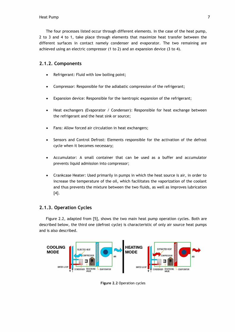
Figure 2.2, adapted from [5], shows the two main heat pump operation cycles. Both are
described below, the third one (defrost cycle) is characteristic of only air source heat pumps
and is also described.
Figure 2.2 Operation cycles
8 State of the Art
Heating Cycle
Compressor and Expansion only ensure proper function when at the input the refrigerant
is in one phase: dry gas or only liquid respectively.
Accordingly, superheated gas at low temperature and pressure is compressed by the
compressor to a high pressure and, consequently, to a high temperature. The heated gas is
then cooled and condensed in the heat exchanger until only liquid, preferably subcooled, is
available. This liquid suffers an isenthalpic expansion in the expansion valve and gets back
into a low pressure and low temperature liquid/gas mixture. The liquid portion is then boiled
in the evaporator a further heated into superheated gas, returning to the compressor.
Cooling Cycle
This is similar to heating cycle but, in this case, heat exchanger functions are switched
because it is intended to remove energy from the recipient. The operation is usually achieved
through a four way valve that changes the order of both heat exchangers in the refrigerant
circuit.
Defrost Cycle
This cycle only applies to heat pumps whose source is the air in the heating cycle.
Sometimes, the evaporator operates at temperatures below 0°C. The humidity allows the
formation of ice layers surrounding this element, which reduces heat transfer and hence the
efficiency of the heat pump.
In order to remove accumulated ice, the system revert its operation, for a short period of
time, to the cooling cycle; the evaporator takes over as condenser, which causes the ice to
melt by heating the element [4]. Also, the introduction of another valve that bypasses the
condenser and expansion valve can be used. With this, gas only passes through the evaporator
and the compressor which highly increases evaporator temperature.
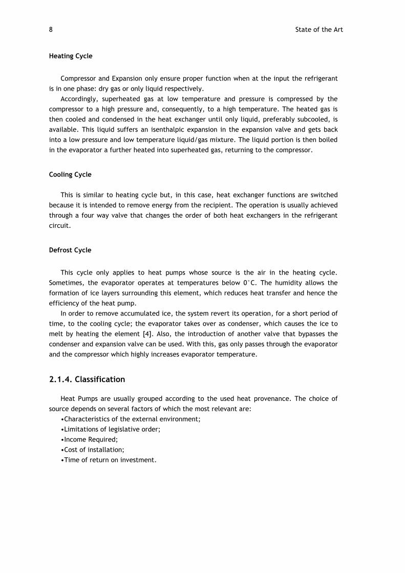
2.1.4. Classification
Heat Pumps are usually grouped according to the used heat provenance. The choice of
source depends on several factors of which the most relevant are:
•Characteristics of the external environment;
•Limitations of legislative order;
•Income Required;
•Cost of installation;
•Time of return on investment.

Heat Pump 9
There are three sources used by heat pumps as illustrated in Figure 2.3 [1].
Figure 2.3 Heat sources
In the classification of heat pumps the fluids involved in the exchange can be used. The
first referenced is the source, and then the receiver. According to this, there are six distinct
types:
Water – Water
Water – Air
Air – Air
Air – Water
Soil – Air
Soil - water
Air
Is always available and can be used without requiring expensive equipment or special
licensing. However, there is a high oscillation of temperature over time and when it passes a
minimum threshold; the pump efficiency may drop dramatically. In this context, in most
installations it is necessary to couple the heat pump with auxiliary heating sources.
Surface Water
Sea water, river or lake may also be used as a heat source. While there are no oscillations
as fast as the air temperature throughout the year, in the colder months, low temperatures
can also induce the same need of auxiliary heating elements.
Underground
Large amount of stored energy can be found, the source is solar near the surface and
geothermal in deeper areas [1]. It can be used by water hole or pit, horizontal collectors,
vertical probes or energy poles. These processes are also illustrated in Figure 2.3.

10 State of the Art
2.1.5. Air Source Heat Pump Domestic Water Heater
The Air Source Heat Pump Water Heater (ASHPWH) is a Air – Water heat pump whose
purpose is to heat water for household or similar proposes. The main characteristic in
detriment of others is the addition of a water tank and auxiliary heating element.
Accumulator of Inertia
In this type of function, in order to reduce the number of times the compressor starts and
the use of energy on expensive tariff time, as well as the regulation of water temperature,
leads to the incorporation of a well insulated water tank.
These tanks are also named as accumulators of inertia and include two main functions:
Hydraulic separation and thermal flywheel [2].
The separation allows for the independence of the hydraulic pump flow to the flow of
heat utilization, this is because hydraulic and thermal requirements are quite different,
especially when used with variable consumption flow rate. Also, the cost of hp is directly
related to its actual power, so an energy reservoir properly sized for the energy requirement
reduces the energy consumption. The numbers 1 and 2 on the figure 2.4, adapted from [1],
represent the two flow regulators for the independent water circuits.
The function of thermal flywheel reduces the number of times the heat pump is
connected, which improves performance and reduces wear on the components. This function
is possible due to the accumulator represented in the picture by the number 3.
Figure 2.4 Heat pump water heater
The Process
In air source heat pump water heater, the evaporator collects energy from the outside
air, which has been pre-heated by the sun and being drawn into the unit by the fan.
According to the cycle explained in 2.1.1, the hot vapor created by the compressor now
enters the condenser where it is surrounded by water from the tank that also flows through
the condenser system with the help of a water pump, causing the heat to be given up to the

Heat Pump 11
cooler water. The cooled refrigerant now returns to its liquid state, although it remains
under high pressure from the compressor.
For better understanding, figure 2.5 [6] is a schematic representation of the steps
described above.
Figure 2.5 Refrigerant circuit
Auxiliary Heating
Compressor decreases dramatically the efficiency with low suction pressures, which leads
to the lowering of COP; so, a maximum ∆T, or maximum difference between inside and
outside temperature should be established. According to that, in the heating mode, there is a
coldest temperature admitted for the heat source, below this point additional heat is
needed. Most early heat pump systems augmented the reversed-refrigerant cycle heating
with resistance electrical heating coils in the air handler. Electrical Resistance heating is not
particularly efficient, however, so as energy became more costly, other auxiliary heat options
were sought. Instead of resistance heating on the evaporator, the coils can be inside the
tank, maximizing the heat transfer, being in direct contact with the heat receiver, and
minimizing losses.
External Auxiliary heating is also used. When the environment conditions are not proper
for the heat pump operation or it is desired a faster heating up, other systems like water
boiler, gas water heater or solar panel can be coupled to the tank providing the necessary
additional heat.
2.1.6. The Coefficient of performance
The instantaneous efficiency of the heat pump refers to well established and controlled
testing conditions. It is given by the coefficient ε and relates mainly to the compressor. It
represents the ratio between the heat transferred to the hot fluid Q and the energy W the
compressor spends plus the auxiliary equipment.
(2.1.1)

12 State of the Art
Actually, the value of ε is the thermal power that can be obtained using 1kW of electrical
power. It is easy to understand that this value increases with decreasing the temperature
difference between the cold source and the fluid. It is easier to transfer energy from 10 º to
30 º than from 10 º to 50 º [2]. But this is not a good indicator of performance for heat
pumps, because only one condition of operation is being measured.
The COP is the coefficient used to compare the performance between heat pumps. It can
be measured according to different European Standards in different conditions. For
certification in some markets, specific standards have to be followed.
European Standard 16147
For domestic hot water units, in France, the EN 16147 is one of those. This one
supersedes the EN 255-3 and determines the COPDHW, instead of the former COP, that is
smaller since heat losses on the water storage tank eliminated. Also five different hot water
consumption (tapping) profiles can be selected during the test, for different tank sizes [7].
Well defined initial and operation conditions are defined as measuring procedures and
minimal requirements for the devices used in.
When the test begins, sequences of operations are made on the heat pump. They consists
in six principal stages:
Heating up period;
Determination of standby power input;
Determination of energy consumption and coefficient of performance for heating
domestic water by using the reference tapping cycles;
Determination of a reference hot water temperature and the maximum quantity
of usable hot water in a single tapping;
Determination of temperature operating range;
Safety tests.
After the third stage it is already possible to know the COP value, which is given by the
formula:
(2.1.2)
Where QTC is the total useful heat during the whole tapping cycle in kWh and WEL-TC is the
total electrical energy consumption during a tapping cycle in kWh.
Seasonal Coefficient of Performance
Another performance indicator is the SCOP. This reports the annual efficiency of the
installation.
Its value is given by the ratio of the heat transferred to the water for one year and the
total energy expended to keep the plant in operation. Thus, its value depends not only on the
performance of the heat pump, but on the entire facility which also includes all the systems
of regulation and distribution of thermal energy.

Heat Pump 13
The Seasonal COP is not easy to determine as it depends on several unstable variables,
such as fluctuation of the cold source temperature, the type of control that manages the
installation or regulation type which generates heat pump. One factor that greatly influences
this value is the number of activations of the heat pump, since during the transient state the
COP is much lower than the referenced [2].
2.2. SuperHeat
The value of SuperHeat is determined by the temperature exceeded by the gas after its
boiling threshold, at the evaporator outlet, that significantly influences the performance of
the refrigeration cycle in the heat pump.
The power exchange is more efficient if the fluid is in the liquid state while it passes
through the evaporator because it is possible to have more fluid mass in contact with the
heat source per unit of time than that which could be found in the gaseous state [8]. In the
ideal case, the total mass of the refrigerant should only be completely boiled at the exit of
the heat exchanger, not just for the reason above but also for the compressor element, to
not incur on premature wear by the admission of fluid in liquid state.
Due to the change in the refrigerant’s boiling threshold by the imposed pressure, it is
possible to control where, in the circuit, the coolant passes totally into the gaseous state. At
this point, so that the phenomenon occurs, the difference between fluid temperature and
saturation threshold must be greater than zero. The cycle efficiency is increased if it is
possible to maintain the SuperHeat value close to 0ºC. However it is imperative to ensure
that the fluid is admitted to the compressor only in the gaseous state adopting a margin of
safety adopted.
Minimum Stable SuperHeat
The concept is defined as a critical minimal degree of SuperHeat at which a refrigeration
system could exhibit unstable operation. It was first proposed by Huelle in 1967 [9].
Huelle observed that the hunting of system parameters often occurred when a low degree
of SuperHeat was set in a Thermostatic Expansion Valve (TXV) controlled evaporator
refrigeration system. Therefore it was assumed that there existed a certain relationship
between Minimum Stable SuperHeat (MSS) and the refrigeration load imposed on the
evaporator. In 1972 introduced conceptually a so-called Minimum Stable SuperHeat signal line
as shown in figure 2.6 [9]. In addition, he considered that the MSS in a refrigeration system
was influenced by the inherited characteristics of the evaporator. In later years it was
experimentally confirmed the existence of such a MSS line, as shown by Huelle [9].

14 State of the Art
Figure 2.6 MSS line. Left and right side correspond to the unstable and stable regions
Normally exists two regions in an evaporator when in operation, namely a two-phase
region and a superheated region, a moving boundary can be assumed separating them. The
moving boundary is called mixture-vapor transition point as shown in figure 2.7 [9].
Researchers have experimentally demonstrated that the mixture-vapor transition point in an
evaporator oscillated in a random manner even under steady operational conditions [9].
Figure 2.7 Refrigerant state on evaporator. Liquid enters on the left and vapor exit on the right side.
Figure 2.8 [10] illustrates the process of phase change that occurs in the refrigerant in
the evaporator. As a result of thermal external action, the evaporation takes place in the
evaporator over which the gas quantity is increased continuously relative to the amount of
liquid. As soon as the gas occupies 10 to 20 times more volume than the liquid in the
evaporator, the speed of the process increases rapidly. Accordingly, the condition at the
evaporator becomes increasingly unstable. What remains at the end of the process is dry and
overheated gas [10].
Figure 2.8 Minimum Stable SuperHeat

SuperHeat 15
Adjusting the load of refrigerant in the evaporator is possible to control where the
unstable zone occurs in the evaporator, guaranteeing that only refrigerant in gaseous state is
admitted by the compressor.
The stable condition (MSS) is generally obtained with a SuperHeat of about 4ºC which can
therefore be characterized as the lower limit of SuperHeat in the stable region. In practice,
stable operating points are usually obtained around 5ºC to 7ºC [10].
2.2.1. How to measure
The SuperHeat is measured expeditiously through two sensors, the pressure-temperature
(PT) table, characteristic of the coolant, and a simple mathematical calculation. An
appropriate sensor measures the pressure at the evaporator outlet; using this value and
according to the PT table of the refrigerant in use is determined the threshold of boiling each
operating condition. Placing a temperature sensor in the same location it is verified the
actual temperature of the gas. The difference between the temperature and the threshold
determines the SuperHeat.
Alternatively it may be measured by the difference between the coolant temperatures at
the outlet of the evaporator and the inlet. This is done assuming two premises. The first
relates that the state of the gas at the inlet of the evaporator is biphasic; this means that
part of the mass is in the gaseous state and the other in its liquid state, than in the
evaporator the rest of the process occurs. The other assumption states that the evaporation
takes place at constant pressure (ideal cycle), and therefore are disregarded any loss of load
on the evaporator.
Through the control point of view, this introduces a concern. The values of the two
temperatures have completely different time constants, as occurs on the TXV which
introduces de hunting phenomena.
In Figure 2.9 [11] is represented the ideal cycle (blue line), and the real situation (red
line). It is notorious what was described in the previous paragraph. Ideally, the heat
exchange in the evaporator is represented by the lower horizontal line, in reality is
represented by the dotted line above, so that it can also be seen that due to these
approximations, the result obtained by the difference of the values of the sensors introduce a
permanent error compared to the real value of SuperHeat. In addition to this fact,
substituting a pressure sensor leads to another temperature disturbance through contact with
the ambient temperature in which the sensor is located. Should also be considered the
reaction time of the sensor to measure variations in the magnitude as well as offset errors
that correspond to them.
Figure 2.9 Refrigeration ideal cycle (blue) versus real cycle (red)

16 State of the Art
Temperature sensors
Thermocouples
Thermocouple is a pair of junctions that are formed from two dissimilar metals. One
junction represents the reference temperature and the other is the temperature to be
measured. They work when a temperature difference causes a voltage, by seebeck effect.
That voltage is, in turn, converted into a temperature reading. TCs are used because they are
inexpensive, rugged and reliable, do not require external power, and can be used over a wide
temperature range.
Thermocouples can achieve good performance and can even be used for short periods of
temperatures. They are also faster than resistance thermometers to react to temperature
changes.
When using TCs, some considerations must be taken. They measure their own
temperature so the temperature of the object must be inferred, and there must be no heat
flow between them. They are also prone to temperature reading mistakes after long time of
use because of insulation resistance loss to thermal conditions or nuclear radiation or even
mechanical interference in the environment. These sensors are electrical conductors so they
must not contact with another source of electricity [12].
Thermistors
As thermocouples, these are also inexpensive, readily available, easy to use, and
adaptable temperature sensors. They are used, however, to take simple temperature
measurements rather than for high temperature applications. Thermistors are made of
semiconductor material with a resistivity that is much sensitive to temperature. These are
widely used as inrush current limiters, temperature sensors, over current protectors, and
self-regulating heating elements.
Thermistors differ from resistance temperature detectors in the material used and the
temperature response. Thermistors can be classified into two types; depending on the sign of
k. If k is positive, the resistance increases with increasing temperature, and the device is
called a PTC. If k is negative, the resistance decreases with increasing temperature, and the
device is called a negative temperature coefficient NTC [12].
Resistance temperature detectors
RTDs are temperature sensors with a resistor that changes the resistance value
simultaneously with temperature changes. Accurate and known for repeatability and
stability, can be used with a wide temperature range.
These sensors have a better accuracy than thermocouples as well as good
interchangeability. RTD sensor is also stable over the long term. With such high-temperature
capabilities, are used often in industrial settings.
Stability is improved when RTDs are made of platinum, which is not affected by corrosion
or oxidation [12].

SuperHeat 17
Infrared sensors
Infrared sensors (IRS) are used to measure surface temperatures ranging from -70 to
1,000°C. IRS convert thermal energy sent from an object in a wavelength range of 0.7 to 20
µm into an electrical signal that converts the signal for display in units of temperature after
the compensation for any ambient temperature [12].
These sensors are used when the target is in motion, in vacuum or hazard, if
temperatures are too high for contact sensors or a fast response is required.
When selecting an infrared option, critical considerations including field of view,
emissivity, spectral response, temperature range, and mounting must be analized.
Pressure sensors
Potentiometric
Potentiometric pressure sensors use a Bourdon tube, capsule, or bellows to drive a wiper
arm on a resistive element. For reliable operation the wiper must bear on the element with
some force, which leads to repeatability and hysteresis errors. These devices are very low
cost and largely used in low-performance applications.
Inductive
Several configurations based on varying inductance or inductive coupling are used in
pressure sensors. They all require AC excitation of the coil(s) and, if a DC output is desired,
subsequent demodulation and filtering is needed. The linear variable differential transformer
(LVDT) types have a fairly low frequency response due to the necessity of driving the moving
core of the differential transformer. The LVDT uses the moving core to vary the inductive
coupling between the transformer primary and secondary [13].
Capacitive
Typically, these use a thin diaphragm as one plate of a capacitor. Applied pressure causes
the diaphragm to deflect and the capacitance to change. This change may not be linear and
is typically on the order of several pico Farads out of a total capacitance of 50-100 pF.
The electronics for signal conditioning should be located close to the sensing element to
prevent errors due to stray capacitance [13].
Piezoelectric
Piezoelectric elements are bi-directional transducers capable of converting stress into an
electric potential and vice versa. They consist of quartz or ceramic materials.
One important factor to remember is that this is a dynamic effect, providing an output
only when the input is changing. This means that these sensors can be used only for varying
pressures.

18 State of the Art
The piezoelectric element has a high-impedance output and care must be taken to avoid
loading the output by the interface electronics. Some of these pressure sensors include an
internal amplifier to provide an easy electrical interface [13].
2.2.2. How to control
SuperHeat control is made regulating the load on the evaporator. This means that if it is
possible to control the flow of refrigerant in this heat exchanger, it is possible to vary the
pressure and with that the boiling point characteristic temperature thus, the SuperHeat
degree according to the definition made above.
Load regulation can be achieved with a variable speed compressor, or through the
expansion device regulation, that is the common solution.
Expansion devices
The expansion device, commonly named as throttle is essential to the operation of the
heat pump.
The valve’s correct sizing and choice of topology play a key role in the improvement of
the refrigerant circuit efficiency. If the system has a fixed speed compressor, this element is
the only available to control the flow of refrigerant admitted on the evaporator as well as the
pressure difference between the high and low side of refrigerant circuit. That is achieved by
restricting the volume of refrigerant to a fraction of the capacity of the compressor.
Controlling this pressure differential allows the refrigerant to boil in the evaporator at the
desired temperature [14].
In this section are presented some of the solutions adopted among time as throttle
devices.
Capillary Tube
As its name implies, this is a system that consists merely in a tube with a length usually
between 0.5 to 6 meters long and with an inside diameter ranging from 0.5 to 2 millimeters.
The operation is summarized by the pressure drop along its length imposing load losses.
As it runs, due to the friction and acceleration the coolant liquid will lose pressure, resulting
in the evaporation of some fraction of it.
Several combinations of internal diameter and length of pipe can be adopted to achieve
the desired effect according to the load applied and the other components of the pump.
However, for a certain combination, is not possible to resize it according variations in the
load or pressures involved.
Usually, the designer of a refrigeration circuit that incorporates a capillary tube chooses
the diameter and length so that the equilibrium corresponds to the desired evaporating
temperature. Then is used a tube longer than the theoretically designed, which results in an
evaporation temperature lower than desired. The final length of the capillary tube is
obtained cutting it successively until the desired balance condition is obtained.
Capillary tubes (figure 2.10) [14] are generally used in smaller systems, with capacities
around of 10 kilowatts and operating conditions practically constant, since any change in the
operation will be reflected in decreased efficiency of the installation [14].

SuperHeat 19
Figure 2.10 Capillary tube
Manually Regulated Expansion Valve
This kind of valve comprises a manually variable area orifice through which the
refrigerant flows and feeds the evaporator. To increase the refrigerant flow running through
it, it is necessary to operate a screw (figure 2.11 [14]) so the valve is opened. To reduce the
valve is closed. The main disadvantage of this expansion valve is the inflexibility to changes
in system load automatically and therefore must be adjusted each the system load,changes.
Should also be opened or closed every time the compressor is turned on or off.
For these reasons, it follows that is only suitable for use in large systems with regular
monitoring and actuation by an operator and where the system load remains nearly constant.
Figure 2.11 Manually regulated expansion valve
Float valve (High Pressure)
A float is placed in the high pressure side of the circuit and immersed in the liquid, which
is the input variable to the valve control.
This type of device operates in a critical load of refrigerant in the system. When the hot
gas is condensed, it flows into an accumulator chamber. Once the liquid level rises in the
chamber the float rises too and the valve opens and allows the liquid refrigerant to pass to
the evaporator. This control allows liquid to pass into the evaporator in equal amount to that
which is condensed. In this way, an overload of refrigerant result in flooding of the

20 State of the Art
compressor and insufficient refrigerant charge will result in underfeeding the evaporator.
Often additional accumulators are used with the aim of making the refrigerant charge less
critical. Figure 2.12 [14] illustrates clearly the principle of operation explained.
Figure 2.12 Float valve (High pressure)
Float valve (low pressure)
The principle of operation of this system is similar to that presented for the high pressure
float valve. The name is due to the placement of the displacer in the low pressure side of the
system as represented on figure 2.13 [14].
This actuator can be used only on systems with flooded type evaporator. The floater is
placed directly on the evaporator or in a suitable adjacent chamber. However, they must be
physically connected to the liquid level in both remains the same under any circumstances.
By increasing the load on the evaporator much liquid is evaporated and the level inside
the float chamber and the evaporator lowers. When this happens, the float level is also
lower, and is allowed more liquid from the high pressure side. When the load is decreased,
the same happens in reverse way.
This type of valve is considered one of the best regulator devices that exist for "Flooded
Systems", due to the excellent control that provides and constructive simplicity that makes it
robust and practically free from damage. It can be applied to any system with flooded
evaporator, whether small or large, and still used with any type of refrigerant.
Figure 2.13 Float valve (low pressure)

SuperHeat 21
Automatic expansion valve
This kind of device is used only in systems with single evaporator, especially for small
capacities and reduced thermal load variations and applicable in almost all refrigerants.
The automatic expansion valve on figure 2.14 [14] operate on the principle of pressure
reducing valve which during operation of the heat pump, retain the evaporator pressure to
the set value regardless of temperature conditions, blocking the flow of refrigerant to the
evaporator.
On the underside is subject to the force of a closing spring, whose adjustment is fixed,
together with the evaporator pressure. At its top the atmospheric pressure acts and the force
of a spring whose tension can be changed by previously adjusting screw situated in the upper
valve.
The greater the spring tension adjustment, the greater the evaporation pressure and vice
versa. Thus, each spring position adjustment, will correspond to a given evaporation
pressure, which will automatically remain constant.
Figure 2.14 Automatic expansion valve
Electric expansion valve
It uses a thermistor to detect the presence of liquid refrigerant at the outlet of the
evaporator (figure 2.15 [14]). When there is the presence of fluid in this state, the
temperature of the thermistor is lower, which reduces resistance, allowing higher current
intensity through the valve to open the fluid channel. This incurs on higher flow, regulating
on this way the outlet temperature of the evaporator.
Figure 2.15 Electric expansion valve

22 State of the Art
Thermostatic expansion valve
The thermostatic expansion valve is the most used regulating device in residential and
commercial applications. Include high efficiency and quick adaptation to various types of
application.
Due to the automatic adjustment and performance, are meant to refrigeration and air
conditioning with one or more evaporators.
Characterized by maintaining relatively constant range of overheating regardless of the
conditions of the system, these promote proper feeding of the liquid in a wide range of
conditions and thermal load, preventing liquid return to the compressor.
The thermostatic expansion valves may be of internal or external equalization depending
on pressure loss in the evaporator.
The biggest drawback of the TXV is the “hunting” phenomena. Hunting is a cyclic
fluctuation due to variation in the SuperHeat of the mass of fluid admitted to the evaporator.
It results from excessive opening and closing of the expansion valve in an attempt to regulate
the SuperHeat. This causes reduced system capacity and efficiency, waste of energy,
decreased comfort, as well as premature degradation of other components of the heat pump,
such as the compressor. The poor dimensioning of the expansion valve, the load with which
the system works, the mass of refrigerant in the circuit or the contact of the bulb
temperature sensor, are some of the factors that can result in the appearance of the hunting.
Due to its construction and principle of operation in closed loop, it is clear that the two
variables implied in the control (pressure and temperature) are acquired with time constants
quite disparate, so if the operating conditions of the system vary relatively quickly is the
appearance of natural fluctuations over a period of stabilization.
Thermostatic expansion valve (internal equalization)
The operation of the thermostatic expansion valve with internal equalization depends on
the pressure of the evaporator and the pressure created by the thermostatic control bulb.
The thermostatic bulb is installed at the outlet of the evaporator in thermal contact with
the suction pipe continuously acquiring the temperature of the refrigerant at the outlet of
the evaporator.
According to the figure 2.16 [14], the pressure Pb acts over the diaphragm (1), which
depends on the temperature of the bulb. On the down side, in contrast, operate the
evaporator pressure Pev and the spring pressure, Pm, through the transmission pin (2).
The movement of the diaphragm, on the downward, moves away the needle from the
orifice, opening up a certain area, allowing the passage of coolant.
The opposite movement, upwards, due to the pressure of the spring (4) reduce the flow
of liquid, which may reach up to complete closure.
It is found that the temperature rise of the bulb and therefore the pressure Pb, or also
lowering the evaporator pressure, Pev, the needle (3) opens, providing increase of liquid
refrigerant flow to the evaporator. However, with pressure drop of the bulb, and an increase
in evaporator pressure, closes the needle passage, throttling the liquid refrigerant to the
evaporator.
Within the chamber beneath the diaphragm and the outlet of the expansion valve
(evaporator inlet) there is a communication path, so that the inlet pressure of the evaporator

SuperHeat 23
is transmitted to the diaphragm Pev. This path is called as the lower valve internal
equalization.
Therefore, on the thermostatic expansion valve with internal equalizer, the evaporation
pressure, Pev is equal to the inlet pressure of the evaporator, than is not considered a loss of
load or resistance on the evaporator.
The thermostatic expansion valve with internal equalization is employed in systems with
small losses (less than 20 kPa). Higher tubing length on the evaporator, leads to greater
losses. Increasing the pressure loss, also the pressure difference between the inlet and outlet
of the evaporator is bigger. This higher pressure will produce at the evaporator inlet, greater
strength below the diaphragm. To remain the valve open, it is necessary that the pressure
Pev increases increasing SuperHeat. To achieve this, is necessary that a part of the
evaporator’s area is used in a less efficient way.
The loss of this area, which is required for evaporation of the coolant, involves several
possible consequences: evaporator partially covered with ice, poor heat transfer, reduced
performance of the whole installation and a malfunction of the expansion valve.
Figure 2.16 Thermostatic expansion valve (internal equalization)
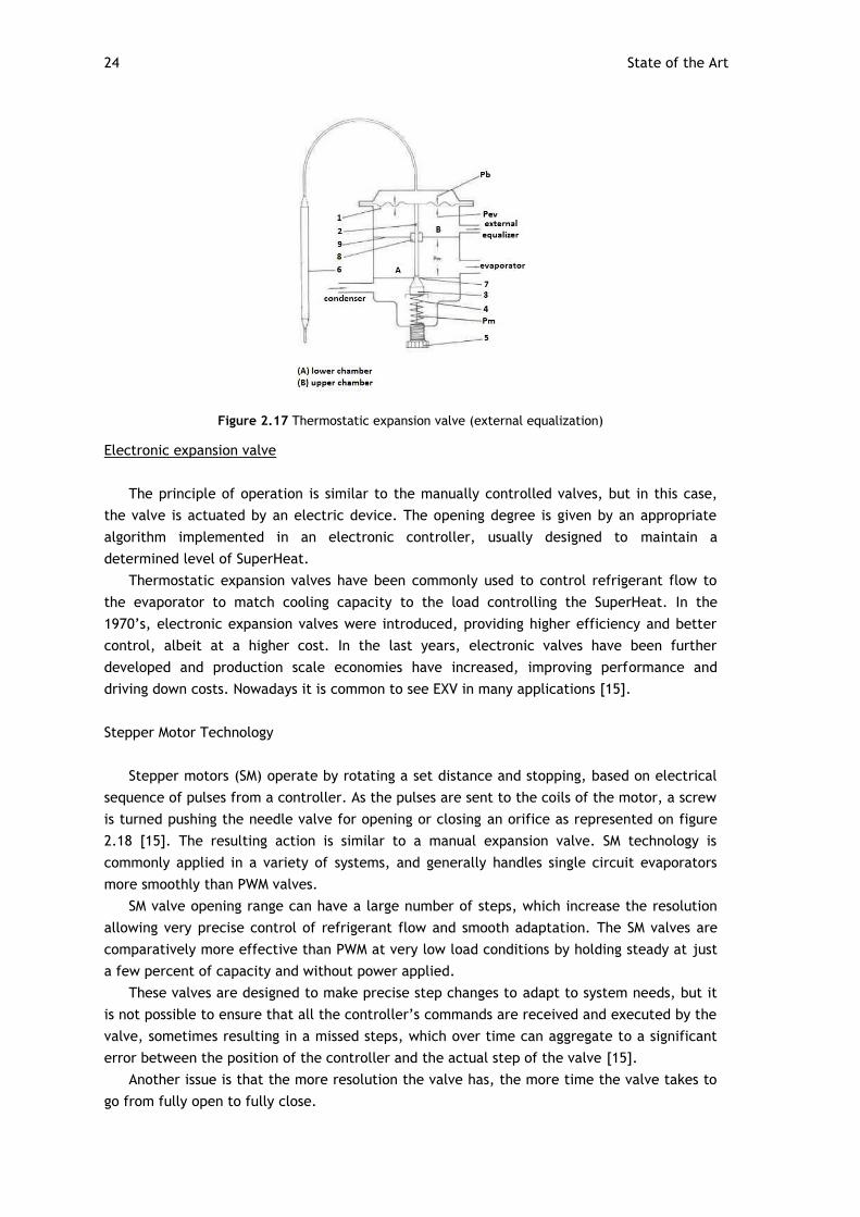
Thermostatic expansion valve (external equalization)
In thermostatic expansion valve with external equalization (figure 2.17 [14]), the inlet
pressure of the evaporator, Pev located in the lower chamber (A) has no contact with the
diaphragm, due to separation by partition wall (9). The pressure of the evaporator Pev
located in the upper chamber (B) is transmitted through the outer pressure equalizer, which
is connected to the outlet of the evaporator. Therefore, the pressure Pev acting beneath the
diaphragm valves equals the pressure of evaporator outlet.
The external equalization eliminates the influence of the flow resistance of the
refrigerant (pressure loss) on the control processes of the thermostatic valves.
In cooling equipment for high load loss (pressure difference between inlet and outlet of
the evaporator greater than 20 kPa), is recommended the use of thermostatic expansion
valves with external equalization of pressure.
24 State of the Art
Figure 2.17 Thermostatic expansion valve (external equalization)
Electronic expansion valve
The principle of operation is similar to the manually controlled valves, but in this case,
the valve is actuated by an electric device. The opening degree is given by an appropriate
algorithm implemented in an electronic controller, usually designed to maintain a
determined level of SuperHeat.
Thermostatic expansion valves have been commonly used to control refrigerant flow to
the evaporator to match cooling capacity to the load controlling the SuperHeat. In the
1970’s, electronic expansion valves were introduced, providing higher efficiency and better
control, albeit at a higher cost. In the last years, electronic valves have been further
developed and production scale economies have increased, improving performance and
driving down costs. Nowadays it is common to see EXV in many applications [15].
Stepper Motor Technology
Stepper motors (SM) operate by rotating a set distance and stopping, based on electrical
sequence of pulses from a controller. As the pulses are sent to the coils of the motor, a screw
is turned pushing the needle valve for opening or closing an orifice as represented on figure
2.18 [15]. The resulting action is similar to a manual expansion valve. SM technology is
commonly applied in a variety of systems, and generally handles single circuit evaporators
more smoothly than PWM valves.
SM valve opening range can have a large number of steps, which increase the resolution
allowing very precise control of refrigerant flow and smooth adaptation. The SM valves are
comparatively more effective than PWM at very low load conditions by holding steady at just
a few percent of capacity and without power applied.
These valves are designed to make precise step changes to adapt to system needs, but it
is not possible to ensure that all the controller’s commands are received and executed by the
valve, sometimes resulting in a missed steps, which over time can aggregate to a significant
error between the position of the controller and the actual step of the valve [15].
Another issue is that the more resolution the valve has, the more time the valve takes to
go from fully open to fully close.

SuperHeat 25
Figure 2.18 Stepper motor electronic expansion valve
Pulse Width Modulation Technology
PWM technology is based on a principle of fully opening and closing a solenoid valve
imposed by a PWM control signal (figure 2.19 [15]). For example, to achieve 50% flow with a
period of six seconds, the valve will open once, remain open for three seconds, close for
three seconds, then the times are continually adapted based on refrigerant flow needs.
As SM, the PWM valves offer unique benefits. The turbulence created by opening and
closing improves evaporator circuit distribution, increasing the usable area of the heat
exchanger. The flow characteristics also improve oil return, which can be a particular
challenge for SM valves in low load conditions. Electrical connections are simpler, with less
wires and simpler controller algorithms. Since these valves are normally closed, they
eliminate the need for an additional solenoid valve. PWM valves are better to adapt to faster
capacity changes, moving from fully closed to fully open and vice versa in milliseconds.
These valves are particularly applied with multi-circuit evaporators. However, the pulsing
current created in the system is a drawback especially in residential applications. Another
negative point of PWM valves is power consumption compared to SM. Stepper Motor valves
consume energy only when changes are required, PWM valves apply current to the coil
holding power for the open portion of the cycle [15].
Figure 2.19 Pulse width modulation expansion valve

26 State of the Art
Electronic controllers
EXV control methods
Not much information is available about the used controller methodologies for the EXV
regulation when tracking the SuperHeat. As expected, the majority of companies don’t give
much information about commercialized controllers. Market giants as Danfoss or Honeywell
only announce “advanced adaptive controllers” [16][17]. Some others, like Sanhua, Dotech or
Carel reveal that controllers are based on linear PID algorithms [18-20].
A constant in these controllers is the inputs used. As seen above, SuperHeat can be
determined by one pressure sensor plus one temperature sensor, or by two temperature
sensors, but every seen market solutions use the first option.
Some studies are published with some other experimented topologies. Liu, Wang and
Chen (2008) [21] proposed an optimal PD controller based on genetic algorithm, in 2010 five
Brazilian engineers developed an adaptive PID controller that according to the operational
condition adjusts the controller gains in real-time [22]. Fuzzy logic based structures like
Fuzzy PD are also presented by some documents [23] [24].
MSS tracking Methods
There are still in market solutions with fixed SuperHeat set point, Dotech Sporlan, Sanhua
or Emerson Climate Technologies are some examples of that [19][20][25][26].
Danfoss and Honeywell are companies that already provide solutions of constant MSS line
tracking. The used algorithm still secret, although Danfoss reveals that the controller is
always downgrading the SuperHeat set-point, until a condition of instability is sensed at the
input (figure 2.20 [17]). At this time the controller increases the set-point until the stability
condition is reached [17].
Figure 2.20 MSS tracking algorithm by Danfoss
Jolly, Tso, Chia and Wong (2000) developed a controller with the same principle of
operation that is described by Danfoss, but the decision of increasing or decreasing the set
point is made based on a fuzzy inference system. The given input is the integral of the error,
sampled in a 60 seconds window, with that is possible to quantify the instability of the
SuperHeat [23].

SuperHeat 27
2.2.3. Conclusions
Thermostatic expansion valve is still largely used by manufacturers, is the cheapest and
most proved solution to achieve satisfactory results when controlling the load in the
refrigerant circuit. But when compared with electronic expansion valves there are several
drawbacks. To improve efficiency by minimizing SuperHeat, to better control humidity by
dynamically managing SH, and to respond more quickly to changing capacity requirements
electronic expansion valves take place.
Figure 2.21 from [15] shows the impact of applying MSS theory that can only be achieved
with EXV: chart shows a simplified TXV SH a fixed setting and the idealization of MSS theory.
Regardless of the choice of PWM or SM valves, applying MSS theory can make systems operate
with less degree of SuperHeat in most applications than those with a fixed SH setting, which
do not achieve optimal efficiency, and can even result in lower efficiency than a TXV. As
such, once a PWM or SM valve is chosen based on the application, it is imperative to use the
adequate control algorithms to ensure the desired results.
Figure 2.21 Minimum Stable SuperHeat theory savings
Overall, PWM has better performance in multiple circuit units where more turbulence
improves refrigerant distribution. On the other hand, on systems with one circuit including
most air-conditioning or heat pump applications, SM valves are the best choice to avoid
excessive pulsation. PWM valves can improve oil return and can adapt more quickly to fast
changes in capacity needs, but SM valves can be more effective in low load conditions and
consume less energy in operation [15].

2.3. Fuzzy Logic
Fuzzy logic is a methodology for control or modeling systems that can be used from small
systems to large and complex networks. It is possible to implement in hardware, software or
both. It is a simple way to be able to set an output based on inaccurate, vague or ambiguous
input information. The method resembles the decision making of a human being, but faster
and more accurate.
The concept was conceived by Lofti Zadeh, professor at the University of Berkeley in
California. It was introduced in 1965, not as a method of control, but as a way of processing
information through inaccurate and incomplete sets.
Zadeh’s theory is based on the fact that people don’t need precise or numerical
information to make decisions, and still be highly capable of providing adaptive control to
systems. If closed loop controllers can be programmed to accept noisy and inaccurate input,
this way it would be even more effective and easy to implement. In 1974, Professor Ebrahim
Mamdani implemented the first controller based on fuzzy logic in the United Kingdom.
Only in the late 70s, fuzzy logic began to be used in control systems due to insufficient
processing capacity regarding the computers of the time. In the early days, the theory was
not widely accepted by the system manufacturers. Later, European and Japanese began to
give him confidence and application. These days, there are numerous applications of the
Lofti Zadeh’s concept. It can be found in areas such as control, supervision and monitoring,
decision support systems, classification of information, computer vision, pattern recognition,
and knowledge-based systems [27].
When using conventional logic, well-defined boundaries are used to characterize sets. In
many situations, this is not the correct approach. For example, to classify the age group of a
person based on their age certain limits are created. If you set the age of 20 years as the
threshold between a young and an adult means a person aged 20 years and one day is no
longer a young man. However, this is not an assignment with meaning in reality.
Fuzzy logic allows defining the degree of membership of a variable to a set using fuzzy
sets for it.
Fuzzy set
Fuzzy set is the expansion of the notion of set, in order to make possible the
representation of concepts defined by fuzzy boundaries, such as those that arise in natural
language or in qualitative concepts. The name of each set is defined by a linguistic variable.
Membership function
The membership function indicates the degree to which a particular concept is a member
of a set. The degree is given by a value between 0 and 1, and when it is 0 indicates that the
variable has no relation with the used set. The degree of membership with value 1 means
that the variable is completely represented by the set.
In figure 2.22 [28] it can be seen that the temperature value represented by the vertical
line intersects two sets and has a high degree of belonging to the set cold (blue) of
approximately 0.8 and a low degree of belonging to the set warm (orange), near the 0,2.

Fuzzy Logic 29
Figure 2.22 Membership function for fuzzy set
Rules
The rule-base is the main part of the FLC. It is formed by a set of logical rules. Rules
determine the relationship between the set of input variables and output fuzzy region. Those
can be either conditional or non-conditional. An example of a proposition, considering u1 and
u2 system inputs and y1 is the output:
If u1 is COLD AND u2 is WARM THEN y1 is MEDIUM.
In this case, the intersection method should be defined to the operator "AND", usually is
used the minimum or the product of the degrees of membership of each variable in the
respective set. Other logical operators may be used like NOT and OR.
Each rule works in the following way: If the conditions of the antecedent are satisfied,
then the conclusions of the consequent are applied.
The importance of the consequent in the controller’s output is calculated by the
antecedent. In the previous example the antecedent corresponds to the underlined part of
the statement. Admitting that the method chosen for the AND operator was the minimum,
the importance of the rule would be the lower value of the degree of belonging of the
variable u1 in the set HOT and the variable u2 in the set COLD. The part that is not
underlined in the proposition is called the consequent.
Usually, in a conventional or fuzzy controller, the inputs are error and error deviation for
set-point tracking. The rules presented in Table 2.1 operate with linguistic labels of the
inputs and output of the Controller. Their purpose is to describe in a qualitative way the
control law of the FLC.
Table 2.1 Example of a Rule-base of a simple FLC
IF error is positive AND error change is approximately
zero
THEN the output is positive
IF error is negative AND error change is approximately
zero
THEN the output is negative
IF error is approximately zero AND error change is
approximately zero
THEN the output is approximately
zero
IF error is approximately zero AND error change is
positive
THEN the output is positive
IF error is approximately zero AND error change is
negative
THEN the output is negative

30 State of the Art
2.3.1. Control architecture
The following scheme (figure 2.23) represents the steps of the fuzzy logic controller in a
block diagram. The function of each block is now presented.
Figure 2.23 Block diagram for fuzzy controller architecture
Fuzzification
The fuzzification is the first stage of the controller. At this time, it is analyzed the
system’s state and acquired the value of the variables of interest. By the intersection with
the fuzzy sets in variables value, related linguistic variables are defined and created regions
according to the degree of membership in each set.
The membership functions can take many forms (figure 2.24 [29]) and should be
appropriate to the type of application and desired result. In the next are examples of
functions that are typically used to describe fuzzy sets.
Figure 2.24 Typical membership functions. Gaussian on the left, triangular on the right side
Inference
At this stage, the rules are analyzed and the ones suitable for the situation through the
inference method will create the resulting region.
Two methods can be considered: Mamdani and Takagi-Sugeno; for both it is necessary to
calculate the weight of each antecedent proposition through as described above.
Mamdani
A region is created through an implication method for each rule. It is generated, for each
consequent linguistic variable; a set whose region occupied is a function of the weight of the
rule.
Next, another method is applied to aggregate all regions generated by each of the active
rules. The resulting region is the entry to the last stage. Figure 2.25 [29] is the illustration of
the process.

Fuzzy Logic 31
Figure 2.25 Mamdani inference block diagram
Takagi-Sugeno
When the chosen inference method is the proposed by Tomohiro Takagi and Michio
Sugeno, the consequent of the proposition is a function (usually linear) of the inputs. After
the determination of each rule’s output, the value is multiplied by the weight of the
corresponding proposition [30]. The controller output corresponds to the average or sum on
this set of results.
Being the outlet a direct function of the system input, the Defuzzification process is
intrinsic to this method as seen in figure 2.26 [29].
Figure 2.26 Takagi-Sugeno inference block diagram

32 State of the Art
Defuzzification
In this final stage the resulting region is converted into the output value of the controller.
It corresponds to the functional link between the regions and the fuzzy expected value.
The objective can be achieved by different methods. Among them the most common is
the "centroid" in which the center of mass of the resulting region will be the output value for
the controller. Other methods such as First-of-maxima or Mean of maxima may be used [30].
These are illustrated in figure 2.27 adapted from [29].
Figure 2.27 Defuzzification methods
2.3.2. Application Examples
Fuzzy logic is already implemented in several areas. Below are some illustrative examples
of them with respective application.
Defense: Systems to support decision making;
Electronics: Automatic exposure control in video cameras;
Aerospace: Altitude control for satellites;
Car: Automatic transmission algorithms;
Signal Processing and Telecommunications: adaptive Filter for nonlinear control of
channel equalization for large spectrum noise;
Industry: Optimization of production;
Navy: Control of autonomous underwater vehicles;
Medical: Diagnosis of diabetes prostate cancer;
Financial: Stock market forecasts.
2.3.3. Why Fuzzy Logic controllers
Since the appearance of control architectures based on fuzzy logic, several reports of
successful implementation of such controllers are published.
A.S. Kamal et al. (1996) applied fuzzy logic to control the refrigerant flow of a
refrigeration system. Its performance has been compared with that of a well-known
commercial controller. Fuzzy logic achieved better control and improved the performance
[31].
Elangeshwaran et al. (2006) explains the advantages of a fuzzy logic based controller over
a PID controller from experimental results. Better control performance, robustness and
overall stability can be expected from the fuzzy controller even though developing and tuning
of the FIS is more intuitive than the PID controller [32].

Fuzzy Logic 33
M. Manjunath et al. (2011) concluded that Fuzzy control combined with conventional PID
controller is a way of intelligent control. Fuzzy adjusts the PID control parameters depending
upon the error. A two input and three output fuzzy adaptive PID control was simulated in
MATLAB environment and the results show that the fuzzy adaptive PID controller have better
stability, small overshoot and fast response [33].
Fuzzy logic is not the only way to reason with ambiguous concepts but it is a good
alternative to model approximation and control engineering. According to the concept, is
easy to enounce some particularities about fuzzy logic:
It can deal with ambiguousness and uncertain information and still producing the
adequate output.
The intuitive knowledge base design allows easier interpretation and adjustments,
even when the user is not a control engineer.
The algorithm is not heavy from the point of view of computational requirement. In
some cases, the controller can be resumed to a Look-up Table with some associated
interpolation method.
Validation, consistency, redundancy and completeness can be checked in rule bases.
The concept is used in many other paradigms, and can also be incorporated with
conventional controllers design, i.e. tuning them for certain plant non linearity due to
universal approximation capabilities. In the case of nonlinear processes which can be
linearized around the operating point, conventional controllers can work successfully, but
these are not optimal in the whole working area [34].
Through figure 2.28 [35] is clear to observe the possibilities that arise from the
integration described above. On the left side is shown a control surface of a conventional
linear controller, on the right the generated surface of a fuzzy logic controller. Adjusting the
fixed gains of the conventional controller the only change in the surface occurs on the slope
of the represented plan, instead, with fuzzy logic is possible to change the shape of the
surface according to the constraints and nonlinearities imposed by the plant.
Figure 2.28 linear controller surface (left) versus nonlinear controller surface (right). The lower axes
refer the inputs and the vertical one is the controller output
2.3.4. Typical fuzzy controller structures
Some of the typical adopted structures results from the junction of i.e. sliding mode or
even conventional Proportional Integrative Derivative (PID) family of controllers. This can be
done either by fuzzy adjustment of the gains of the conventional controller, according to the

34 State of the Art
operating condition (fuzzy gain scheduling), or by the emulation of the controller law using
knowledge base rule systems (Fuzzy like).
Fuzzy Gain Scheduling
This type of controller utilizes a rule based auxiliary scheme for gain scheduling issues.
It is implemented expecting that operating regions are associated with overlapping
membership functions of the fuzzy sets defined in the scheduling variable space and that a
fuzzy inference mechanism is used to dynamically interpolate the controller parameters
around region boundaries based on known local parameters.
According to state variables of the system, the operating point is determined. In some
cases, it can be done through the same variables used in the main conventional controller;
others use new state variables so the Fuzzy Logic Knowledge Base (FLKB) is capable of
adjusting the gains of the main structure.
Gain scheduling PID with fuzzy knowledge base is exemplified on the block diagram of the
figure 2.29. In this example, the two state variables are the inputs to the fuzzy inference
mechanism that provides gain adaptation to the three components of the PID.
Figure 2.29 Gain scheduling PID controller (fuzzy based)
The control law of the conventional parallel PID is given by the equation (2.3.1), where
Kp, Kd, and Ki are the static gains of the controller.
(2.3.1)
When α, β and θ are the three outputs of the Fuzzy Logic Knowledge Base, the output is:
(2.3.2)
Where:
(2.3.3)
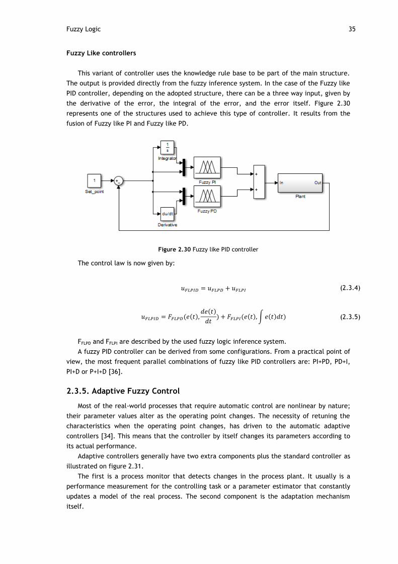
Fuzzy Logic 35
Fuzzy Like controllers
This variant of controller uses the knowledge rule base to be part of the main structure.
The output is provided directly from the fuzzy inference system. In the case of the Fuzzy like
PID controller, depending on the adopted structure, there can be a three way input, given by
the derivative of the error, the integral of the error, and the error itself. Figure 2.30
represents one of the structures used to achieve this type of controller. It results from the
fusion of Fuzzy like PI and Fuzzy like PD.
Figure 2.30 Fuzzy like PID controller
The control law is now given by:
(2.3.4)
(2.3.5)
FFLPD and FFLPI are described by the used fuzzy logic inference system.
A fuzzy PID controller can be derived from some configurations. From a practical point of
view, the most frequent parallel combinations of fuzzy like PID controllers are: PI+PD, PD+I,
PI+D or P+I+D [36].
2.3.5. Adaptive Fuzzy Control
Most of the real-world processes that require automatic control are nonlinear by nature;
their parameter values alter as the operating point changes. The necessity of retuning the
characteristics when the operating point changes, has driven to the automatic adaptive
controllers [34]. This means that the controller by itself changes its parameters according to
its actual performance.
Adaptive controllers generally have two extra components plus the standard controller as
illustrated on figure 2.31.
The first is a process monitor that detects changes in the process plant. It usually is a
performance measurement for the controlling task or a parameter estimator that constantly
updates a model of the real process. The second component is the adaptation mechanism
itself.

36 State of the Art
Figure 2.31 Adaptive fuzzy controller
Performance Measures
The choice of one or more performance measures depends on the type of response the
control system designer wishes to achieve. The final output of the performance monitor, as
seen by the adaptation mechanism, is either the actual values of the measurements, or a
performance index derived from the variable readings.
For the regulatory control problem, where the aim is to keep a process variable on its
specified set-point, many performance-related variables can be used:
Overshoot;
Rise time;
Settling time;
Decay ratio;
Frequency of transient oscillations;
Integral of the square error;
Integral of the absolute value of the error;
Integral of the time-weighted absolute error;
Gain and phase margins.
Adaptation Mechanism
The adaptation mechanism must modify the controller parameters to improve the
controller performance according to the information of the output from the process monitor.
There are three ways of adaptation. The first is altering scaling factors; is similar to adjusting
the gain in a PID controller but in this case, the input or output variables are multiplied by a
scaling factor. With this is possible to change the sensitivity of the controller to the inputs or
the actuation gain.
The second is modifying fuzzy set definitions; this one allows small changes in the shape
of the fuzzy sets in order to improve the performance of the controller.
The third is the self organizing methodology, which the main purpose is to change the
rules from the knowledge base by trying to identify the rules responsible for the poor
performance and replacing them for better ones.

Chapter 3
SuperHeat Modeling and Simulation
The third chapter describes the used methodology to achieve a model capable of
describing the behavior of the SuperHeat according to the opening degree of the expansion
valve in all operating conditions. The controller architecture and its simulation are also
presented.
It is divided in four sections. The first one introduces the company’s given prototype and
describes its key features for the proposed objective.
Then, the adopted solution for SuperHeat modeling is presented and justified and is made
a description of how the different variables and parameters were estimated and determined.
The validation of the model is also presented in this section.
The third section is related to the controller architecture and the reasons for the adopted
solution.
Finally, some considerations are made about the integration of the model with the
controller in the simulation and the results are shown.
3.1. System Specification
Bosch provided a prototype for the project which is a complete heat pump similar to the
production ones, with the particularity of the expansion device. In this case, instead of the
usual thermostatic expansion valve, there is an electronic expansion valve.
According to the single circuit evaporator, the low mass of refrigerant used, the possible
residential application of the heat pump and energy consumption issues, a Stepper Motor EXV
is used rater than a Pulse Width Modulation EXV which is in agreement with section 2.2 of this
document.
There were also added two Negative Temperature Coefficient temperature sensors, the
same as used in water or air temperature measures for the heat pump control, but these ones
are for sensing the Evaporator inlet and outlet temperatures for the estimation of the
SuperHeat.
The choice of two temperature sensors instead of one for pressure and the other for
temperature is due to the production savings, and the avoidance of major modifications in
the heat pumps that are already in production.

38 SuperHeat Modeling and Simulation
NTC sensors have suitable characteristics for the application. The necessary range of
temperatures is not wide and the resolution achieved is enough when few tenths of degrees
are not a much relevant change in SuperHeat.
In this prototype, variable water pump flow and ventilator speed are available. With this,
is easily and faster to emulate changes on the operating conditions, like water or air
temperature without having to change the actual variable physically that consumes a lot of
energy and time. The control of these elements is possible through direct action in the
Human Machine Interface (HMI).
3.1.1. Main Characteristics
Figure 3.1 schematically identifies the main components of the heat pump. Also identifies
the inputs and outputs of the Central Processing Unit (CPU).
Figure 3.1 System specification
(1) Top Temperature sensor (9) Compressor (Fixed Speed)
(2) Bottom Temperature sensor (10) Electronic Expansion Valve (SM)
(3) Air Temperature sensor (11) High Pressure Switch
(4) Fins Temperature sensor (12) Water Pump (Variable Flow)
(5) Evaporator Outlet Temperature sensor (13) Fan (Variable Speed)
(6) Evaporator Inlet Temperature sensor (14) Water inlet
(7) Condenser (15) Water outlet
(8) Evaporator (Single Circuit)

System Specification 39
3.1.2. Temperature Sensor
Type: NTC thermistor;
Maximum temperature: 100ºC;
Minimum temperature: -30ºC;
Rated resistance: 10kΩ ± 3% @ 25ºC;
Maximum deviation: 4.6% @ -30ºC;
Thermal time constant (in water): 8s.
Acquisition circuit is represented in figure 3.2:
Figure 3.2 NTC acquisition circuit
3.1.3. Expansion Valve
Type: 4 Phase Stepper Motor;
Resolution: 500 steps;
Operating range: 40 to 500 steps (experimentally determined)
Max flow: 1.8l/m;
Minimum temperature: -30ºC;
Maximum temperature: 70ºC;
Design pressure: 42 bar (600 psi).
Driver circuit is represented in figure 3.3:
Figure 3.3 Electronic expansion valve driver circuit

40 SuperHeat Modeling and Simulation
3.1.4. FAN
AC Supply: 230VAC, single-phase;
Control: PWM;
Max speed: 2580 rpm;
Resolution: 0..255 (duty cycle: 0..100%);
Operating range: 50 to 200 steps.
In order to determine the usable range of the PWM applied to the fan, PWM value was
decreased until the fan stops, and then increased until the rpm change is no longer
noticeable.
3.1.5. Water pump
DC Supply: 12V;
Control: PWM;
Resolution: 0..255 (duty cycle: 0..100%);
Operating Range: 40 to 110 steps.
With a flow to frequency transducer, a test was made in order to determine the actual
flow of the DC water pump according to the selected PWM and the usable range of values.
The results are shown in table 3.1 and in a graphical way from figure 3.4. The water pump
stops when PWM step is under 40, and a significant increase in the Power/Flow ratio occurs
above 110 steps on the water flow.
Figure 3.4 Water pump flow rate chart
Table 3.1 Water pump flow rate
PWM Value U Current Power Frequency Flow
49 8.4 0.12 1.01 11.8 1.464
52 9 0.12 1.08 14.3 1.702
73 9.6 0.2 1.92 28.7 3.073
83 10.1 0.24 2.42 32.7 3.453
96 10.6 0.29 3.07 37 3.863
103 10.9 0.31 3.38 38.7 4.024
110 11.6 0.41 4.76 46 4.719

System Specification 41
3.1.6. HMI/Central Processor Unit
(Only relevant characteristics for SuperHeat control is presented)
Temperature acquisition sensibility: 0.1ºC;
Stepper actuation period: 8ms;
Expansion valve controller period 250ms.
3.2. System Modeling
The determination of the mathematical model of a complete generic heat pump is a long
process that involves highly nonlinear phenomenon and complex thermodynamic equations.
Looking at the area of research, this is not within the objective, considering that the model is
only necessary to characterize the SuperHeat behavior.
Accordingly, an alternative to the complete model that is capable of describe only the
behavior of the necessary variables, with sufficient accuracy, and that enables the design of
an appropriate solution has been searched.
The transient response of SuperHeat as a function of mass flow rate passing through the
expansion valve can be approximated by a First Order Transfer Function plus Time Delay
(FOTFTD) [37-39][22]. Thus, for this purpose it becomes unnecessary the elaboration of a
computationally heavy mathematical model for the whole heat pump. Through this model
approximation, factors like temperature sensors time, delay or offset errors are already
considered in the parameters determination.
Since the characteristic output of the impulse response is similar to the one represented
on Figure 3.5, K, τ and θ are extrapolated graphically as illustrated.
Figure 3.5 Graphical transfer function parameters determination
1. The process gain is determined by the ratio between the total variation of the
temperature (KM), and the value of the step in the actuator (M):
2. Draw the tangent at the inflection point of the step response. The intersection with
the time axis indicates the delay of the system.
3. The intersection of the tangent with the line KM indicates the time instant must be
used to determine the time constant, since at this point t = τ + θ.

42 SuperHeat Modeling and Simulation
Analytical determination is also possible:
1. Define T0 as the time when the change in actuator occurs;
2. Locate where the measured process variable first shows a clear initial response to the
step change, and name it as T1;
3. Locate where the measured process variable reaches 63.2% of its total final change
and call it T2;
4. Time constant is the difference between T2 and T1;
5. Time delay is the difference between T1 and T0;
6. Process gain is the ratio between the total variation of the temperature and the step
in the actuator.
Minimum Stable SuperHeat
The Minimum Stable SuperHeat condition, so that the system remains stable, will not be
considered in the SuperHeat model. The philosophy that is intended for the controller regards
the robustness and applicability of the algorithm in different heat pumps.
Two possible options could be considered to solve the problem of Minimum Stable
SuperHeat.
The first is the determination of specific curve of the threshold for stable operation for
each heat pump. This would involve intensive and controlled tests to encompass all possible
operating ranges. However, it was still imperative a safety margin more or less extensive,
depending on the accuracy and the reliability of sensors used, as well as corresponding
manufacturing process i.e. the control of load applied to the refrigerant circuit. Factors that
change the dynamics of the refrigerant circuit would also result in a change of the MSS line.
This adopted margin result in higher SH set-point and consequently the loss of system
efficiency.
The second one and adopted, monitors the evolution of SuperHeat along the time and
changes the SH set-point accordingly to its stability. Thus there is no need of determining
parameters for each pump produced or adoption of a safety margin, so that the SuperHeat is
maintained at a level which confers some instability when it crosses the line with MSS,
however enables a lower SH value and a more efficient operation for the heat pump. The
algorithm will be illustrated in detail in chapter 4, sub-section 4.1.3.
3.2.1. Parameter determination
According to reference [22], the gain and time constant are variable parameters that
depend on the operating conditions of the heat pump, particularly in the evaporation
temperature and the inlet temperature of the water in the condenser, as shown in figure 3.6.
Figure 3.6 High level model diagram

System Modeling 43
Assuming the above, an assay was made in which the variation in the fan speed and the
water pump would produce the same effect that is derived from the variation of air and
water temperature. A software version that allows the manual setting of the expansion valve
was flashed in the CPU, this means that it was possible to manually choose a value from 0 to
500 in which the EXV should remain. Variations in valve’s position were defined and the
corresponding change of SuperHeat was analyzed.
During this first test, it was found that whatever the conditions applied, SuperHeat was
above the MSS values only when the valve position was lower than 80 steps. This indicates
that the valve was oversized, which would cause less refined control by the waste of partial
valve’s aperture range.
After a new sizing done, it was determined that an EXV with maximum flow of 1.3 L/min
should be used in that refrigerant circuit. The expansion valve was replaced for this new one
and the tests were repeated. The essay was processed and the delay, time constant and gain
for each test were determined.
According to the results, some conclusions were drawn:
The aperture of the expansion valve has to be reduced to maintain the same
SuperHeat value as the evaporation temperature is decreased. This is explained by
the reduction of energy exchanged with the air that will slow down the process of
evaporation inside the evaporator for the same flow of coolant, so the mass of fluid
inside the heat exchanger has to be reduced.
The same happens when the water temperature increases but, in this case is due to
the growth of the difference between the condenser and the evaporator
temperatures that also increases the refrigerant fluid pressure which changes the
flow. In this case, more mass of refrigerant passes through the evaporator if the
aperture of the EXV is maintained.
If the valve is in a defined step with stable SuperHeat, even if the operating
conditions are maintained, a temporarily change in its aperture makes the SuperHeat
value slightly different from the last one verified in that step on a random way.
The delay in SuperHeat response to step changes increases randomly when MSS line is
nearby.
The SuperHeat value suffers from an offset transformation when operation condition
changes for the same step in the EXV, this was measured for every tests.
In the opposite way to what was said in reference [22], that the gain depends on the
operating condition, it was verified that it actually changed among tests but it does
not follow any pattern.
Looking at valve’s datasheet it is verified that the flow characteristic according to the
opening is not linear and therefore the determination of parameters through different ranges
of steps in the valve opening would invalidate these results for gain parameter
determination.
Once again the tests were repeated, but this time with a fixed change form step 60 to 80
and from 80 to 60 which represents a fall and a rise respectively in SuperHeat value.
Table 3.2 represents the calculated gain of the system according to changes in the water
flow and air flow. Values are within the scale units and ranges defined of sub-section 3.1.4
and 3.1.5.

44 SuperHeat Modeling and Simulation
Table 3.2 Gain results
rise Water Pump Speed fall Water Pump Speed
FA
N S
peed Gain 40 65 85 110
FA
N S
peed Gain 40 65 85 110
50 5,5 4,2 4,1 5,7 50 5,3 4,7 4,6 5,2
80 4,6 5,3 4,5 4,4 80 4,8 5,1 4,9 5,0
127 5,3 5,2 4,6 4,8 127 5,1 4,8 4,7 5,4
200 4,8 5,0 5,1 4,5 200 5,1 4,9 4,9 5,2
The results indicate that there are no noticeable changes in gain values when operation
conditions change, but in the time constant determination a tendency is reflected. The next
table represents it in for each test of the essay.
Table 3.3 Time constant results
rise Water Pump Speed fall Water Pump Speed
FA
N S
peed Time 40 65 85 110
FA
N S
peed Time 40 65 85 110
50 43 41 36 39 50 34 38 35 37
80 42 35 29 31 80 30 31 27 28
127 34 34 29 26 127 27 27 24 24
200 33 29 27 24 200 26 23 20 19
A significant reduction of values as the water pump flow and air flow increase is present;
in this case, it is also clear the decrease in the time constant for values in the fall tests when
compared to the rise ones.
The resulting values for the delay time were practically constant, with an average value
of 4 seconds.
The non-linearity of the aperture of the expansion valve was also tested. With fixed
speed in fan and water pump, a new essay was made that consists in the evaluation of the
SuperHeat value, from the minimum stable value to maximum possible by gradually closing
the EXV and registering its position and corresponding SH value. Both fan and water pump
were in maximum speed according to the above conclusions in order to achieve the maximum
step possible before the SuperHeat value hits the MSS line. Even in this condition the
maximum stable step achieved was 240 of 500.
The result is represented in the chart of figure 3.7 by the red dots and is clear the non-
linearity of the SH as a function of the EXV aperture. The variation in gain, referred in [22], is
probably due to the opening characteristic of the expansion valves and not for de change in
the operation conditions. From the four references that support the modeling of SuperHeat,
[22] is the only that refer the gain variation.
Due to the introduction of this fact in the simulation model this, and the necessity of
approximating the gain for the steps above 240, the characteristic was represented by a
potential curve (black line) fitting. In figure 3.7 that process is lustrated. The blue dots
represent the estimated values in the same step value of the SuperHeat ones.

System Modeling 45
Figure 3.7 SuperHeat according to EXV step
Table 3.4 completes the chart above with the analytic values of the ones represented. In
some steps the error of the estimation value is high, but according to the behavior of the
existing random offset of the SuperHeat even in same operating conditions, this is not
considered relevant.
Table 3.4 SuperHeat for EXV step chart values
EXV step
SuperHeat (ºC)
Approximation (ºC)
Error (ºC)
Gain
500 1,2 0,0024
450 1,4 0,0030
400 1,6 0,0039
370 1,7 0,0047
340 1,9 0,0057
310 2,2 0,0071
280 2,5 0,0089
260 2,8 0,0106
240 3,4 3,1 0,3 0,0127
220 3,6 3,4 0,2 0,0156
200 3,9 3,9 0,0 0,0194
180 4,1 4,4 -0,3 0,0247
160 4,2 5,2 -1,0 0,0324
140 5 6,2 -1,2 0,0440
120 8,6 7,5 1,1 0,0627
100 11,3 9,5 1,8 0,0953
80 14,4 12,7 1,7 0,1593
60 19,7 18,5 1,2 0,3086
50 23,2 23,5 -0,3 0,4692
40 27,8 31,3 -3,5 0,7837

46 SuperHeat Modeling and Simulation
On figure 3.8, the determined gain according to actual step is represented. It is given by
the quotient of the aperture and the estimated SuperHeat.
Figure 3.8 Gain for EXV step
3.2.2. The model
While determination of parameters, important system behavior conclusions were made.
Accordingly, the model of the system will count on some characteristics:
The operating conditions are given by the values of the chosen Fan Speed (FS) and for
the Water Pump speed (WP);
Time constant is approximated by the interpolation of two look up tables (LUT), one
for the rising SH response and the other to the fall;
Offset is also given by one LUT according to the two inputs for the operating
conditions;
LUT’s contain the exact experimentally determined values from the essays;
Gain is given according to the position step by the fitted potential function.
The block diagram of the model implemented in Simulink is in figure 3.9, the blocks are
in numbered groups, and the description of each is below the figure.
Figure 3.9 SuperHeat model

System Modeling 47
1- First order transfer function with time delay;
2- Time constant look up tables;
3- Rise or fall behavior of SuperHeat detection for switching LUT;
4- Saturation block for EXV step limitation;
5- Offset LUT.
3.3. Model Validation
Model validation was made through the comparison between the results of essay and
simulation of the model using the same operation conditions and step variation. In figure 3.10
one of these tests is shown.
Figure 3.10 Simulation (blue) versus real (red) step response
In the situation above, fan speed was set to 200, and water pump speed to 85. The step
on the valve’s aperture is from 90 to 190.
From table 3.4, the step 90 (initial condition) is in a zone were theoretical values have
the largest error (approximately 1.7ºC). In this essay, the measured delay was of 3 seconds,
and time constant is similar from the two plots. In the final condition, the step 190 presents
an error of about 0.4ºC.
In other tests, when chosen steps on potential curve approximation steps have less
deviation from the real value some results are almost coincident.
From the results, it can be concluded that simulation produce results that are closer to
the real conditions attending to all the random behaviors reported and to the errors from the
gain approximation function.
3.4. Controller Architecture
Several considerations were made to the choice of controller type. Functional constraints
such as limited processing capacity and memory storage are present. Allied to that, the
easiness of adaptation for new systems has to be guaranteed.
“Fuzzy like” solutions are proper due to structural simplicity that makes the adaptation
for new heat pumps possible only by few adjustments, like the change of gains and the range
for inputs if the SuperHeat response changes significantly.

48 SuperHeat Modeling and Simulation
Also, the ECU memory and processor limitations increase the necessity in the
simplification of the controller. Fuzzy like controller, according to inference system, can be
expressed by a Look up table, whose size can be adjusted according available memory, and
an adequate interpolation method, that complexity can be adjusted meeting, the processor
speed limitations.
As in conventional controllers, there are variants of 2 terms (PD or PI) and 3 terms (PID)
in “Fuzzy like” controllers.
Fuzzy PD control is known to be less used than PI because it is more difficult to remove
the steady state error. However, PI type control usually gives poor performance in transient
response for higher order process due to the internal integration operation [40].
Fuzzy like PID controller needs three inputs, it makes the rule base larger which is a
drawback in memory issues. Also, the performance over Fuzzy PI is not much improved
because of the small influence of the acceleration error in general.
With a little change in the structure, the performance and memory usage of the “Fuzzy
like PID” can be improved by the avoidance of using the acceleration of error input. This is a
hybrid velocity/position Fuzzy PID.
Hybrid Fuzzy Logic PID
This kind of controller uses the combination of a velocity type PI and a position type PD.
Fuzzy PD controller generates control output from error and change in error and PI
generates an incremental output from the same inputs. Figure 3.11 represents by block
diagram the proposed controller.
Figure 3.11 Hybrid Fuzzy Logic PID schematic
The output is given by:
(3.4.1)
Where:
(3.4.2)
(3.4.3)
(3.4.4)
The gains can be expressed as:
(3.4.5)
(3.4.6)
(3.4.7)

Controller Simulation 49
3.5. Controller Simulation
Two stages of the controller simulation are presented. In the first, controller is
considered without characteristic or implementation constraints. The second considers every
identified restriction at the implementation for the evaluation of the introduced drawbacks.
In both, the water pump speed is increasing from maximum to minimum speed to
introduce the tank heating up condition. Fan speed is fixed in 127 which correspond to actual
heat pump working mode.
As in the real operation, initial valve position is defined to half aperture (250 steps).
3.5.1. High Level Simulation
The high level simulation uses only the process model and the controller structure that is
achieved by linear block representation and the use of the Fuzzy Logic Controller from the
Fuzzy Logic Toolbox. It has also added a gain scheduling function to the original structure
called EXV that actually is the inverse function of the gain to linearize the aperture of the
expansion valve. Figure 3.12 represents the model used for simulation.
Figure 3.12 High level controller
After the tuning of parameters and adjustments in membership function shape and
values, the best compromise between tracking speed and overshooting is represented in
figure 3.13. The set point values are changed every 1000 seconds. Initially, tracking point is
set to 7ºC, after the 1000 seconds it changes to 3ºC. When simulation reaches 2000 seconds,
the set-point is changed to 13ºC. The last step is on 3000 seconds and SP is defined to 4ºC.
Figure 3.13 High level simulation

50 SuperHeat Modeling and Simulation
The maximum overshoot is of 0.2ºC, and in a step change of 10ºC, the controller takes
250s until stabilization.
3.5.2. Implementation Level Simulation
This level of simulation considers all the constraints derived by the system
characteristics. In this, instead of the block of the Fuzzy Logic Toolbox, a look up table of
two inputs and one output is used. The two look up entries have 20 steps for each. Linear
interpolation method is used, as in the real controller.
The EXV gain scheduling is also given by a LUT instead of the potential function.
Sensor resolution in the CPU acquisition, period of the controller cycle, LUT’s and
derivative method are the same used in implementation. The block diagram of this simulation
is represented in the next figure.
Figure 3.14 Implementation level controller
In the simulation of figure 3.15, the procedure is the same of the above. There were not
also gain changes.
Figure 3.15 Implementation level simulation
3.6. Resume
SuperHeat behavior, above the threshold where the influence of the MSS is not
significant, can be approximated by a First Order Transfer Function plus Time Delay with

Resume 51
variable time constant. To describe the non-linearity of the expansion valve, a gain
scheduling block from the electronic expansion valve has to be introduced.
According to the random behaviors of superheat, there is a sufficient level of correlation
between the designed model and real system.
Due to the simplicity of the architecture, easiness of adaptation for new heat pumps with
different parameters, and known good performance on systems described by FOTFTD, “fuzzy
like PID” topology has been adopted.
Besides the introduction of the system constraints, the controller still able to tracking
set-point in accurate way without noticeable performance decrease from the ideal model.
The maximum overshoot was of 0.2ºC, and in a step change of 10ºC, the controller taken
about 250s until stabilization. These results induce that this solution should be capable of
maintain SuperHeat close to set point, with sufficient accuracy, when implemented in the
hardware of the heat pump.

52

Chapter 4
Implementation and Results
This fourth chapter describes how the solution is implemented in the real system for
testing and the final results achieved through the developed project are shown.
The fuzzy logic controller response in transient, start up and steady set-point operation
are presented. According to the results, elations are made. The behavior of the Minimum
Stable SuperHeat tracking is also stated.
A comparison with a similar heat pump which the only difference is in the expansion valve
that is a thermostatic one is presented. SuperHeat controller efficiency is compared as well
as the heating performance of both heat pumps.
4.1. Implementation
This section is divided in three sub-sections representing the actuation method of the
expansion valve, the fuzzy logic controller and lastly the Minimum Stable SuperHeat tracking
procedure.
The algorithms are implemented in C++, and the rest of the code already made for the
heat pump control suffered only little modifications for the integration of the new expansion
valve and the two new sensors. Debugging was made through the presentation of the interest
variables directly on the HMI. Initially inputs were given through potentiometers connected
instead of the NTC temperature sensors and at a later stage during the actual operation of
the heat-pump.
4.1.1. Expansion Valve Actuation
The actuation of the expansion valve is achieved through the activation or deactivation of
four outputs in the Electronic Control Unit. As presented on sub-section 3.1.3, the stepper
motor has four built-in coils, and through the correct sequence of each one’s excitation the
valve’s orifice is opened or closed. Table 4.1 is given by the manufacturer and shows the
correct sequence of steps for movement.

54 Implementation and Results
Table 4.1 Coil activation order
Coil 1 2 3 4 5 6 7 8
Φ1 ON ON OFF OFF OFF OFF OFF ON
Φ2 OFF ON ON ON OFF OFF OFF OFF
Φ3 OFF OFF OFF ON ON ON OFF OFF
Φ4 OFF OFF OFF OFF OFF ON ON ON
To open the expansion valve, the activation of steps is made from the number 1 to 8. To
close, the inverse sequence must be taken.
In order to know the current step of the valve, an initialization procedure should be
adopted. Every time the compressor starts, the valve completely closes through the
application of 560 pulses in sequence from the number 8 to 1 and then the used variable for
the position is reset. At this point, for opening, the sequence should start from the step 1 and
every step applied should increment or decrement in one unit the position according to
opening or closing operation.
When the controller orders a new position to the valve, it is calculated the difference
between the actual step and the ordered. The Electronic Control Unit starts to give pulses in
the correct order until the difference is null.
Valve steps are limited for maximum and minimum values; beyond those the valve is no
longer activated.
Due to a mechanical break on the valve, when it doesn’t need to be moved, no excitation
on the coils are applied, which allows to reduce the power consumption.
The control task has a constant period of 8ms, so the maximum number of step changes
for one second is 125.
4.1.2. Fuzzy Logic Controller
Fuzzy logic controller of figure 4.1 is the one responsible for tracking the set point, and it
was previously simulated as seen in chapter 3. The algorithm runs every 250ms and is now
briefly explained.
Figure 4.1 Implemented fuzzy logic controller
1- The Temperature of the two NTC sensors is given by pre-made functions that linearly
interpolate the value of read voltage with the manufacturer’s established constants.
In order to use only integer variables, to allocate less memory, the value is already
multiplied by 10

Implementation 55
2- The difference between the evaporator outlet and inlet temperatures represents the
SuperHeat. Signal e(t) is now determined through the deviation of the SuperHeat
from the set-point that is also multiplied by 10.
3- The error rate de(t) is calculated by the difference between samples taken every
three seconds and divided by 3.
4- The two Look-Up Tables present in simulation have outputs in order of the decimal,
so those were copied and all the values were multiplied by 10.
5- The value of the actual EXV position is taken as input for the same function that
interpolates the NTC values, but in this case is used on the EXV gain LUT. The output
is multiplied by both KI and KP constants.
6- A bilinear interpolation function was created and interpolates the Fuzzy LUT. The
values of the two inputs error and error rate are limited to the boundaries of the look
up table.
7- The result of step 6 is multiplied by the new KI from step 5 and integrated through
the multiplication with 0.25 due to the period of the control task.
8- The result of step 6 is multiplied by the new KP from step 5 and summed with the
result from step 7.
9- The last step is the division with the scale factor that results from every
multiplication.
4.1.3. Minimum Stable SuperHeat Algorithm
As previously referenced in section 3.2, set-point tracking is made trough Minimum Stable
SuperHeat.
The MSS algorithm can be divided into two parts. The first senses the system instability,
by measuring the amplitude of the oscillations of SuperHeat around the set point. If the
oscillations are above a certain threshold, this means that the set-point is close to the MSS,
then a status flag will be activated until the stability condition is achieved.
The second refers a state machine that according to the system condition, changes the
set-point having in consideration the system stability and the proximity to the MSS line.
System Instability Detection
Instability condition is defined through the detection of the inflection points in the signal
e(t). In the schematic representation of figure 4.2, the procedure is easy to understand.
Figure 4.2 Instability determination overview

56 Implementation and Results
When e(t) crosses the SH SP (SuperHeat Set-Point) line, it starts the detection to the
biggest absolute value until the line is crossed again. The minimum (light blue) is detected
when the error is below zero and the maximum (orange) when it is above.
In situations like in the figure 4.3, if only the procedure above was made, the orange line
would be like the dashed one, which doesn’t make sense. So, a new condition was adopted: If
the maximum or minimum value maintain unaltered for more than X time, and if the error
change within Y time is too small, then the max value is null.
Figure 4.3 Instability detection (particular case zoomed in)
Set Point Control
A state machine works directly on the control of the SP value for the SuperHeat in order
to keep it close to the minimum stable.
Whenever the compressor is started, the smaller the flow resistance of the fluid in the
refrigerant circuit, the lower the inertia to overcome and therefore the lower the consumed
power. To avoid current peaks at startup, expansion valve is set to a large aperture position
and remains so for some time in order to make the system reach some stable operation.
Only at this point the SuperHeat control is activated and the state machine starts. When
the heat pump starts, SH is set to a value that should be stable.
State INIT: A fixed value for the last set-point is maintained until the stability
condition is reached. At this time, the next state is 1. If the system spend time more
than sufficient to stabilize the SH and it remains unstable, the next state will be 2.
State 1: The value of the set point is gradually reduced until it is determined the
condition of instability. At this point, the state set point is overlapped with the line
of minimum stable SuperHeat, the next state is 2.
State 2: If instability is detected, the machine immediately goes to state 3. If it stays
a large period in this state, it can mean that the line of MSS can be far, so that a new
search should be made, and that the state is changed to 1.
State 3: Is made a high increase in the set point value, and waits until the SuperHeat
returns to stability. As in the INIT state, if spend more time than the sufficient to

Implementation 57
stabilize the SH and the system remains unstable, the next state will be 2. Otherwise,
the set point value will be gradually decremented whose total value of the decrease
is only a fraction of the initial increment. In this last process if the instability is
reached, the state is changed immediately to 2.
In any of these states, if the water temperature in the bottom of the tank decreases
by more than a certain limit for a given tapping, it can indicate that the value of the
MSS changed. Then the state is changed to INIT, in order to the process restarts the
tracking of the line MSS again.
The diagram of figure 4.4 with the table 4.2 illustrates expeditiously the above process.
Figure 4.4 State machine diagram

58 Implementation and Results
Table 4.2 State and transition description
Number Transition Description
2 SuperHeat is stable
5 SuperHeat is unstable or State ended the task
3,4 SuperHeat is unstable
1,6 Large time on state
7,8,9 Bottom tank temperature decreased
Number Action Description
INIT Controller starts
1 Gradually decreases SuperHeat set point
2 Do nothing
3 Increases set-point and waits enough time to stabilize, then gradually decreases
until a fraction of the initial increment
4.2. Fuzzy Logic Controller Analysis
For testing the controller’s start-up, transient and steady operation, a software version
without the MSS tracking algorithm was loaded. It allowed changing the set point manually.
During the test, the ambient temperature is approximately constant but water pump flow and
fan speed were changed as indicator of the robustness of the controller.
The first condition verified is the start up (figure 4.5). Controller’s constants, KP and KI,
tuning was made also according to this to reach a good compromise between overshoot and
settling speed to the set point. To reduce even more the overshoot in this case, the gains
should be much lowered what would influence the rest of the operation in the heat pump
because this is the only case when super seat value departs from a value near zero, so it will
cross the whole unstable zone which changes radically the dynamics of the system.
In figure, the green line represents the position of the EXV, in steps. Even before the
controller starts, the compressor is already working and the EXV is steady with large
aperture, so the SuperHeat, represented by the red line, is below 0ºC. The controller starts
at the moment the variation in the EXV is verified.
In the presented start up, the overshoot was of approximately 6 degrees, and followed by
undershoot of only 1 degree. After approximately three minutes since the controller starts,
the SuperHeat is on the set-point (blue line).
Figure 4.5 Start up condition

Fuzzy Logic Controller Analysis 59
Steady operation is shown on figure 4.6. SuperHeat and Set-Point are represented through
the colors red and green respectively. Due to the sensibility of the temperature input, only
variations of tens of degree are evident. It was not expected to achieve a perfect line for
SuperHeat shape because the phase change of a fluid has a randomly unstable behavior [9],
so oscillations, even with steady operation conditions actuators, will happen.
It is found low resolution of the EXV when it is with little aperture (blue line). Only one
step causes a variation in SuperHeat of more than it should. In the right side of the chart it is
seen that the valve tries to settle in a position that makes SH in the desired value but that
intermediate step does not exist so the controller is alternating between two positions. This
induces that the EXV continues oversized.
Figure 4.6 Steady state operation
The orange line is the temperature of the water in the bottom of the tank. In the 25
minutes represented in the chart, it increased about three degrees, and is possible to see in
EXV position a sudden decrease of the average value. Figure 4.7 has large time range(about
three and half hours) and with that, the above statement is more clear to check.
Figure 4.7 Steady state operation (zoomed out)

60 Implementation and Results
The assumption of sub section 3.2.1 that the water temperature rise makes the expansion
valve to work on more close position in order to maintain the SuperHeat value is once again
experimentally verified.
The next two charts are representative of the transient tracking. In the first one (figure
4.8), the set point (blue line) is initially in 6 degrees and no undershooting of SH (red line) is
verified, a set point change happens, to five degrees, but this time an undershoot of about
0.3 degrees is verified. As the set-point is getting closer to de minimum stable, the influence
of the MSS is more evident and the undershooting is getting higher, as there was an attraction
force bellow. Even with this condition, the controller was able to stabilize SuperHeat in five
degrees after about 180 seconds.
Figure 4.8 Response to set-point fall
The second chart (figure 4.9) is from a set point rise when SuperHeat was unstable. Set-
point changed from 4.5ºC to 6.5ºC. In this condition, a bit of the presented effect of the
SuperHeat instability zone is felt, and overshoot of about 0.6ºC. The controller managed to
stabilize SuperHeat after about 140 seconds of the set-point change.
Figure 4.9 Response to se-point rise (while unstable)

Minimum Stable SuperHeat Algorithm Analysis 61
4.3. Minimum Stable SuperHeat Algorithm Analysis
The MSS algorithm is based on three states during the heat pump operation, except if the
temperature of the water in the bottom of the tank falls more than 5°C. In Figure 4.10, those
are represented. The red line represents the current value of SuperHeat and the blue one the
set point along the time.
At the beginning of the time scale, it is found that SH is about to enter a state of
instability. At this time, state 2 is active. Due to the instability the algorithm immediately
passes the active state to 3 and an abrupt increment in set-point happens.
Sufficient time passes until the stabilization, when the system is given as stable set point
starts to decrease slowly. When the decrement is completely set next state is 2 however, the
system is with a little of instability, but the amplitude in oscillation is not sufficient to
consider the system unstable, so the value of the set point is maintained.
After a long period with a constant value of set-point, the algorithm returns to track the
MSS switching from state 2 to state 1 and begins to decrement the SP. When in instability set-
point is increased again and, after stabilization, returns to decrement a little bit less than
the previous increment. This time, in opposite, when set-point stops decreasing, the system
is not stable so the next state will be the number 2 but will pass directly to 3 and the
procedure is repeated.
Lowering the temperature of water in tank, as well as the restart of the compressor was
tested and the algorithm returned to the initial state as desired.
Figure 4.10 Minimum Stable SuperHeat tracking
4.4. TXV versus EXV on SuperHeat Control
The SuperHeat controller ability is now compared between the current solution and the
developed one. In the figure 4.11 bellow, it is presented the SuperHeat of the system with a
TXV on blue and with EXV with the projected controller in red during the first heating up
performed on the COP test.
One of the inputs of TXV is the pressure that has almost negligible time constant, so the
actuation is faster to sense fluctuations and that allows the TXV working in less degree of
SuperHeat. Although, using this lower set-point, introduces constant oscillations, with high
frequency, that are a big drawback in efficiency and promote the wear of the compressor.

62 Implementation and Results
The higher set-point operation reduces performance, but in the opposite way, there is an
increase due to SuperHeat stability. So the EXV combines system stability and less wear of
the remaining elements of the heat pump
Figure 4.11 SuperHeat behavior during total heating up (TXV on blue, EXV on red)
4.5. Coefficient of Performance
COP test, according to standard EN 16147, on the final version of the project was
conducted and relevant results are now presented. With this procedure, not only the
performance index but also other parameters such as the total time or energy consumed
during the heating are determined. As seen in sub-section 2.1.6 all operating conditions are
the same for each test, and maintained with small admissible deviations. With these
indicators, it is possible to assess the gains that the changes made to the heat pump allow,
for comparison of results from previously performed tests.
Figure 4.12 below represents two curves of a complete heating of the water inside the
tank, the red is the result of the project’s heat pump, and the blue of a similar heat pump
with TXV, the same used for SuperHeat behavior comparing on the earlier section.
In the conditions of this test, when water temperature reaches about 17ºC, the
evaporator is frozen, so the heat pump switches to defrost cycle. At this time, the water
pump is turned off. Due to the position of the water temperature sensor, readings suddenly
decrease until heat pump returns to the normal heating mode.
Figure 4.12 Water temperature on heating up (TXV on blue, EXV on red)

Coefficient of Performance 63
The heating up curves are practically superposed, and therefore the spent times for each
solution are similar. Only a small difference exists, being this new solution faster in 2:30 min.
The energy consumption, in total duration of test, was also reduced, but this time
significantly, compared to the TXV solution. In figure 4.13 both electric power consumption
profiles are traced and the overall power consumption decrease is evident. During the test,
savings reached 2.31%.
Figure 4.13 Electric power consumption on heating up (TXV on blue, EXV on red)
The maintained performance even with the reduced consumption represents efficient
operation which allows an increase in Coefficient of Performance value of 2.14%.
4.6. Resume
Through the results, it is possible to conclude that every stage of the controller is
implemented successfully. It was tested in a variety of different conditions in which the start
up, transient and steady operation were verified with good results and according with the
simulations made.
The application of the MSS algorithm makes the average value of SuperHeat higher,
although there is a much significant reduction in the oscillation amplitude and frequency.
With this, reduction on compressor wear as well as more stable system operation is achieved.
After realization of the COP test, it is verified that the performance is similar to the
thermostatic expansion valve solution, but efficiency is increased by the reduction of power
consumption. This leads to the expected rise in the Coefficient of Performance indicator.

64

Chapter 5
Conclusions
5.1. Epilogue
In this dissertation a solution to the control of an Electronic Expansion Valve integrated
on a Heat Pump was designed and implemented. Design process is described and results on
simulation and real operation are shown.
Initially a search was done on the main issues addressed throughout the project. The
same fell on matters related to the heat pump and control of processes. An introduction to
the operation of a heat pump, different types and existing components that constitute it are
presented. The focus is oriented ASHPWH due to the type of pump where the controller will
be implemented.
Incorporating an EXV is intended for more effective control of the specific phenomenon
called SuperHeat, so a study thorough the influence variables and its behavior was made. It
was determined that its response is highly nonlinear and there is a minimum threshold which
must not be exceeded due to system instability and consequent loss of efficiency. The
amount of SuperHeat should be kept as low as possible but ensuring stability.
Solutions already on the market and other studies developed and published articles were
evaluated as well as components used for sensing and actuation. It appears that thermostatic
expansion valves are still being used on a large scale because it is a cheap solution and
operating proven, however there are several negative effects when compared with electronic
expansion valves. For a more efficient and dynamic control of the SuperHeat EXV should be
used and, in systems with reduced capacity, the stepper motor electronic valve should be
chosen because it prevents excessive pulse and promotes efficiency by less energy
consumption compared with the PWM.
Two common ways are used for measuring the SuperHeat; through one pressure sensor
and one temperature sensor or using two temperature sensors. The great majority of
solutions use the first option, however, in attempt to reduce costs, it was given preference to
the first and the investment is made in the control algorithm towards gain advantage at this
point.
The initial study also passed by the controller logic. Due to the nonlinearity of the process
a suitable nonlinear controller should be used. Restrictions in terms of processing speed and

66 Conclusions
memory led to controllers based on fuzzy logic of the “Fuzzy Like” type, by the structural
and implementation simplicity, to be adopted. The delay in Superheat’s step response and
the necessity for a follow-up set point with a low steady state error were decisive to the
choice of a controller with the components proportional, derivative and integrative.
By the complexity that involves a model able to describe the operation of a heat pump,
just to collect a state variable, it was used an approximation by a first order transfer function
with time delay that describes the behavior of SuperHeat by varying the flow passing through
the expansion valve. Experimentally it was found that the gain and delay of the transfer
function is nearly constant in different operating conditions of the pump, but the time
constant is variable. Due to the nonlinearity of the expansion valve opening when its value is
given by the step position and not by the maximum mass flow rate, a variable gain should be
considered according to the position of the valve.
Upon experimental determination of the parameters, the model was built with all
identified system constraints and nonlinearities. It was verified enough correlation and so,
able for being used in the simulation and tuning the controller.
In simulation, the adopted topology proves to be adequate, with a quick response
considering the time constants involved and minimum error in steady-state and also low
overshoot.
Once deployed, and real tested, the controller continued to verify the effectiveness of
set point tracking. However, as expected in situations where the SuperHeat is lower than the
minimum stable it is impossible for any set-point stabilization.
The SuperHeat minimum threshold tracking algorithm was effective, keeping a low set
point, without compromising system stability.
After realization of the Coefficient of Performance tests, comparing the results with a
similar heat pump which the only difference is the use thermostatic expansion device, it was
verified that the performance is identical but with more efficient operation, with the
reduction in 2.3% in electricity consumption which contributed to an increase of 2.1% in the
value of COP in respect to the previous solution.
Looking at logged data of both during the operation, with the EXV there is an increase in
the absolute value of SuperHeat, but with a significant reduction in oscillation, which
contributes to system stability and durability of the heat pump components.
Strategies presented by some manufacturers for this type of components and solutions
announce higher efficiency gains with the use of electronic expansion valves. To heat pumps
with similar capacities as the employed one, only the energy spent in the operation of the
expansion valve represents an increase of approximately 2% in the system energy
consumption. Significant gains should only be observed in solutions which the capacity
involved is higher so the valve actuation losses will not be significant.
5.2. Future Work
There are still work that can be done in order to improve the use of the electronic expansion
valve. Some suggestions are now presented:
Reduce the expansion valve dimension for refined control and less power
consumption during operation. Even with the change from the 1.8l/m to 1.3l/m the
EXV is still oversized.

Future Work 67
Exhaustive Fuzzy PID parameters tuning for better transient set-point tracking which
can promote the reduction of stabilization times in the Minimum Stable SuperHeat
algorithm.
Exhaustive testing of MSS algorithm parameters in order to achieve better
performance by lowering SuperHeat set-point, but maintaining stability. Also adopt
solution that reduces the valve actuation to decrease power consumption.
Explore the variation in controller performance by changes in the sensors resolution
and controller frequency.
Testing the controller with a pressure transducer instead of two temperature sensors.
By the reduced time constant in acquisition, improvements in control can possibly be
made.
Implementation of the SuperHeat controller in the Suction Line Heat Exchanger
(SLHX) solution. This is an addition of another Heat Exchanger in the heat pump that
allows the evaporator to work with less SuperHeat which increases efficiency and
that cannot be controlled with the thermostatic expansion valve.

68

References & Bibliography
[1]. Doninelli, M. a. M. (2009). As Bombas de Calor. Hidraulica, Caleffi.
[2]. Andreas Zottl, R. N., Marek Miara (2012). Benchmarking method of seasonal performance, Intelligent Energy Europe. Technical Report.
[3]. (2008). Refrigeration. Rankine. New World Encyclopedia, New World Encyclopedia contributors.
[4]. Inc., C. R. (2007). The Heat Pump Reference Guide. Renewal and Enhancement of the 4th Edition Heat Pump Reference Guide. Mississauga, Ontario.
[5]. Heat Pump Designs, Apogee Interactive. Inc. Commercial Energy Systems Library, Retrieved 14-04-2013, from http://www.apogee.net.
[6]. Source Heat Pumps, Retrieved 23-03-2013, from http://www.idealheating.com.
[7]. Standardization, E. C. F. (2011). Heat pumps with eletrically driven compressors. Testing and requirements for marking of domestic hot water units. CEN/CENELEC, Technical Committee CEN/TC 113. EN 16147.
[8]. MacDonald, V. N. Refrigeration Cycle Optimization. Evaporator Superheat Control System, Freescale. Technical article.
[9]. Yiming, C. (2007). The Operational Stability of a Refrigeration System Having a Variable-speed Compressor (VSC). Department of Building Services Engineering. The Hong Kong Polytechnic University.
[10]. Jørgensen, F. (2005). The expansion valve’s potentials and limitations. Nordborg, Denmark, Danfoss.
[11]. França, F. Controle Térmico de Ambientes, DE – FEM Unicamp.
[12]. Mathas, C. (2011). "Temperature Sensors - The Basics." Retrieved 16-03-2013 from http://www.digikey.com.
[13]. Bicking, R. E. (1998). "Fundamentals of Pressure Sensor Technology." Retrieved 23-04-2013, from http://www.sensorsmag.com.
[14]. Dispositivos Medidores. D. d. E. Mecânica, Universidade Federal do Paraná, pages: 113-125.

70 References & Bibliography
[15]. Holloway, J. (2013). “Which electronic expansion valve technology is right for you?, Danfoss.
[16]. (2010). SuperHeat Controller - SHC, Honeywell GmbH.
[17]. (2010). Danfoss – the pioneer in electronic expansion valve control, Danfoss.
[18]. Tommaso Ferrarese, B. L., Gianluigi Bacilieri Intelligent control system with integrated electronic expansion valves in an air-conditioning system operating at a Telecom telephone exchange, Carel Engineering.
[19]. (2010). Electronic Expansion Valve Control Unit, DOTECH sensing and control.
[20]. (2012). Controller for EEV, SANHUA International Europe.
[21]. Liu Tingrui, W. J., Chen Guangqing "Simulation & control of Electronic Expansion Valve." Pacific-Asia Workshop on Computational Intelligence and Industrial Application, Vol. 1, pages: 123-126.
[22]. A.Maia, M. d. A. S., R.Nicolau N. Koury, L. Machado, A. Eduardo (2010). Control of an Electronic Expansion Valve Using an Adaptive PID Controller. International Refrigeration and Air Conditioning Conference. Purdue University.
[23]. P. G. Jolly, C. P. T., P. K. Chia, Y. W. Wong (2000). Intelligent Control to Reduce Superheat Hunting and Optimize Evaporator Performance in Container Refrigeration. Singapore, School of Mechanical and Production Engineering, Vol. 6, pages: 243-255, Nanyang Technological University.
[24]. Liu Tingrui, C. G., Wang Jidai (2008). "Autocontrol of Electronic Expansion Valve Based on Optimal Fuzzy PD Controller." Second International Conference on Genetic and Evolutionary Computing, pages: 352-355.
[25]. (2013). Electronic Residential Superheat Control, SPORLAN Division.
[26]. (2010). Stand-alone Superheat Controller, EMERSON Climate Technologies.
[27]. D.Kaehler, S. (2008). "Fuzzy Logic Tutorial." Encoder – The newsletter of Seattle Robotics Society.
[28]. M. Meghana, V. Rani.(2010) “Fuzzy Logic and its importance in Whizzy Devices”, Electronics Engineering Papers, S.R Engineering College, Warangal.
[29]. Introduction to Fuzzy Logic and Fuzzy Control, (2008) Faculdade de Engenharia da Universidade do Porto. Course materials.
[30]. J.Yen, R. L. (1999). Fuzzy Logic: Intelligence, Control and Information, Prentice Hall, New Jersey.
[31]. J.Y.M. Cheung, A. S. K. (1996). Fuzzy Logic Control of Refrigerant Flow. International Conference on Control, UKACC, Vol. 1, pages: 125-130
[32]. Elangeshwaran Pathmanathan, R. I.(2010) "Development and Implementation of Fuzzy Logic Controller for Flow Control Application." International Conference on Intelligent and Advanced Systems (ICIAS), pages: 1-6.
71
[33]. R. Manoj Manjunath, S. J. R. (2011). "Fuzzy Adaptive PID for Flow Control System based on OPC." IJCA Computational Science - New Dimensions & Perspectives, Vol. 1, pages: 5-8.
[34]. D.Driankov, H.Hellendoorn, M.Reinfrank. (1996). An Introduction to Fuzzy Control. Springer-Verlag New York.
[35]. (2013). "Using Lookup Table in Simulink to Implement Fuzzy PID Controller." Retrieved 16-06-2013, from http://www.mathworks.com.
[36]. Pivonika, P. (2002). "Comparative Analysis of Fuzzy PI/PD/PID Controller Based on Classical PID Controller Approach." Proceedings of the 2002 IEEE International Conference on Fuzzy Systems, Vol.1 pages: 541-546. [37]. Roozbeh Izadi-Zamanabadi, K. V., Hamed Mojallali, Henrik Rasmussen, Jakob Stoustrup "Evaporator unit as a benchmark for Plug and Play and fault tolerant control.” Fault detection, Supervision and Safety of Technical Processes, Vol.8, pages: 701-706.
[38]. C. Aprea, C. R. (2000). "Experimental analysis of a transfer function for an air cooled evaporator." Applied Thermal Engineering, Vol.21, pages 481-493.
[39]. Hua Li, S.-K. J., Jung-In Yoon, Sam-Sang You (2008). "An empirical model for independent control of variable speed refrigeration system." Applied Thermal Engineering, Vol.28, pages: 1918-1924.
[40]. H.X. Li, H. B. G. (1995). Enhanced Methods of Fuzzy Logic Control. Proceedings of the IEEE International Conference on Fuzzy Systems, pages: 331-336.
[41]. (2012). First order plus dead time model, Universitá Degli Studi di Salerno Facoltà di Ingegneria.
[42]. George K. I. Mann, B.-G. H., Raymond G. Gosine (1999). "Analysis of Direct Action Fuzzy PID Controller Structures." Transactions on Systems,MAN, and Cybernatics, Vol. 29, pages: 371-388.
[43]. Gómez, F. J. R. M. a. E. V. (2005). Bombas de calor y energías renovables en edificios.
[44]. Pedro Albertos, A. S. (1998). "Fuzzy Logic Controllers Advantages and Drawbacks."
[45]. Ronald R. Yager, D.Filev. (1994). Essentials of Fuzzy Modeling and Control. John Wiley & Sons,New York.
[46]. Tsung-Tai Huang, H.-Y. C., Jin-Jye Lin (1999). "A Fuzzy PID Controller Being Like Parameter Varying PID." IEEE International Fuzzy Systems Conference Proceedings, Vol. 1, pages: 269-276.
[47]. Vineet KUMAR, K. P. S. R., Vandna GUPTA (2008). "Real-Time Performance Evaluation of a Fuzzy PI + Fuzzy PD Controller for Liquid-Level Process." International Journal Of Intelligent Control and Systems, Vol.13, pages: 89-96.