Advanced Foundation Engineering Prof. Kousik Deb

Department of Civil Engineering Indian Institute of Technology, Kharagpur

Lecture - 9

Shallow Foundation: Bearing Capacity - IV

Hello, now last class I have discussed about the footing, which is loaded eccentrically. I

have discussed about the one way eccentricity and two way eccentricity. Now, on this

class I will discuss the how to calculate the bearing capacity of the soil in layer condition

now, as we know that soil is not a homogeneous soil. Because but but till now the most

of the things that I have discussed is to calculate the bearing capacity of homogeneous

soil. Now, soil is our layer type of material. So, now the property of the soil according to

depth is not same, it is changing. Now, if the soil is the is the condition is the layered

condition then how to calculate the bearing capacity of these layered soil, that I will

discuss in this class.

(Refer Slide Time: 01:16)

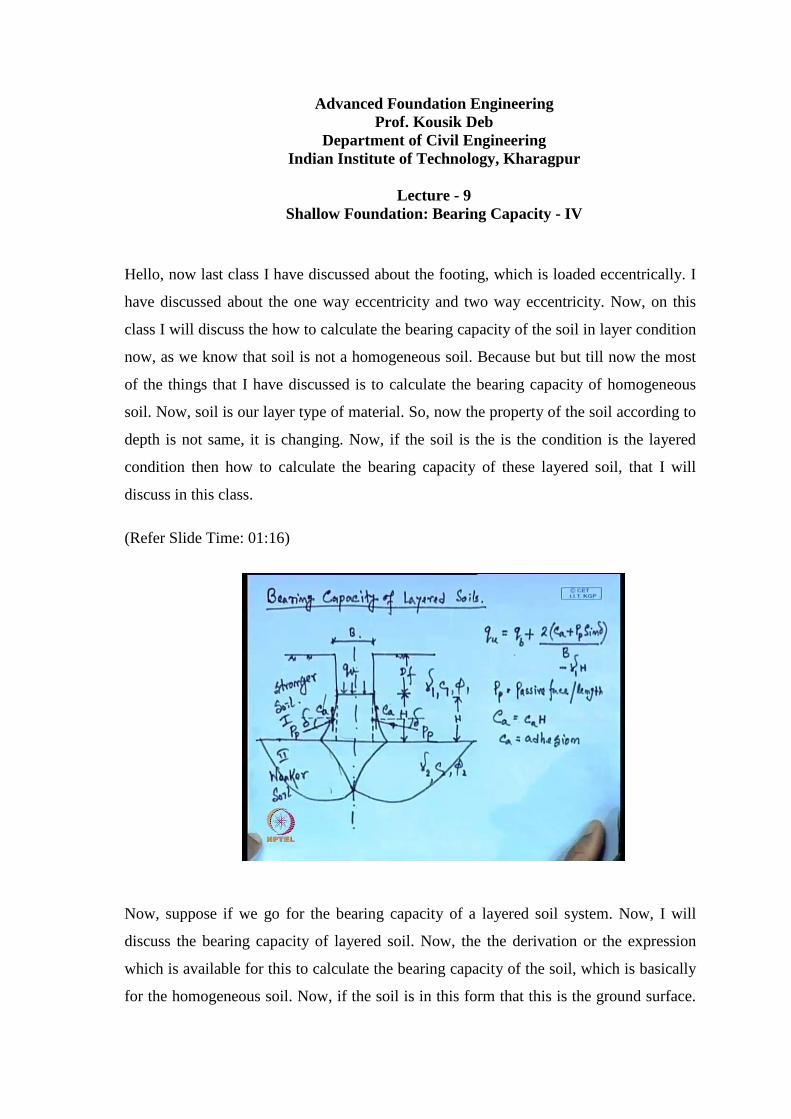
Now, suppose if we go for the bearing capacity of a layered soil system. Now, I will

discuss the bearing capacity of layered soil. Now, the the derivation or the expression

which is available for this to calculate the bearing capacity of the soil, which is basically

for the homogeneous soil. Now, if the soil is in this form that this is the ground surface.

Here we are applying this footing, this is a ground surface and this is width of the

footing, and this is the depth of the footing D f. Now, we are considering the two soil

layer, this is one layer which is the strong soil, which is stronger soil or layer 1 and layer

2, which is weaker soil. So, this is the stronger soil and this is the weaker soil.

Then how to calculate the bearing capacity of this soil condition and suppose the this is

the properties gamma 1 C 1 and phi 1 for the layer is layer 1 and gamma 2 C 2 and phi 2

for layer 2. Now if this stronger soil, if this is the inter phase if the stronger soil and one

thing that the depth of this stronger soil from this base of the foundation is H that is the,

up to this the up to H depth from the base of the foundation is the stronger soil then

weaker soil.

Now, if the depth H is relatively small, then what will happen? Then then there will be a

punching type of shear failure for this stronger soil layer and then general shear failure

for the weaker soil. So, suppose this is the punching type of failure surface, punching

shear failure type of failure surface for this strong soil and then this is the general failure

surface which is expected for the weaker surface. So, these type of failure surface that

will tabular, so now if I draw one line vertical line. So, what are the forces which is

acting suppose in this because here it is the general shear type of failure so that means,

we can calculate this is the q bottom or the bottom layer and for this punching shear

failure what are the forces that is acting.

So, first is the adjacency a, this is which is acting two side of this layer because suppose

this is the one block which is falling or that means, this is the size. Now, another thing

the passive resistance the surrounding soil; that will provide for this zone or this zone

that is the passive resistance P p, which is acting at angle of delta. Similarly, this side

also this is the P p which is acting another angle delta. So, this two types of force which

which is these are are acting here both this is the central line. So, one is the adhesion in

the both side of this layer and passive resistance coming from the soil of this side and

soil from this side which is acting at the angle of delta to the perpendicular of this line.

This is P p, P p is the passive resistance. Another thing that if this H value, here if this H

which is the distance which is depth of this layer or from the base of the footing is

relatively small then we will get this type of failure surface.

Now, if the distance is relatively large then we will get the most of the failure surface

will be in the stronger layer. So, the failure surface of the effect of the loading intensity

of the footing load will not act suppose this is the footing load that is q ultimate. That

effect will not go to the second layer or the weaker soil layer. So, most of the failure

surface or will be located at the stronger layer. In that case the general expression for the

shear failure expression, general shear failure expression for the or for homogeneous soil

or single layer soil that we can use to determine the loading of the or bearing capacity of

the soil. Now, if it is relatively small then we will go for this approach. Now, one thing is

that that this value. So, if I go for the different loading condition.

So, what will be the different loading condition for this case. So, first we will calculate

the q u for the loading condition, the vertical load q u which is acting in the downward

directions, that is equal to the perpendicular load that is acting so the resistance that q u

is the total load bearing capacity. This is the some portion of the resistance that we will

get from the bottom layer and some portion we will get from the top layer. So, this is the

summation of the resistance or the load which is carrying by some portion by the strong

layer and some portion by the weak layer or the bottom layer and the top layer. Suppose

in the bottom layer it is as usual the general shear failure. So, we can write this is the

resistance that is q bottom. So, q bottom is the load carrying capacity of this bottom layer

or the resistance that is coming from this bottom layer, plus the resistance that is given

by this top layer that will be 2 into C a, it is the adhesion 2 means one from this side,

another from this side plus because here P p which acting as the delta.

So, the sine component that will act in the upward direction, so that will give the upward

resistance, so that is P p into sine delta. So, that means these are the upward forces

divided by B, because these things acting as a width of P minus gamma 1 into H, because

this is the, this load or the q that is acting here gamma 1 into H that is the surcharge

below the base of the foundation up to the second layer or up to the starting of the second

layer or up to the end of the first layer. So, that is the total force. That means, the

contribution of the q is the contribution from the bottom soil, plus the contribution from

the top layer and minus this value surcharge that we are detecting. Because these

surcharge we will not consider as a contribution because it is it was existing previously.

So, now these are the total load. Now, here P p we can write that is passive force per unit

area. So, that is the passive force per unit length. Here we can write that C a is equal to

small c a into H. Because C a is the total load that is total resistance due adhesion and

small c a is the adhesion, which is per meter. So, that is the total and then as it is acting

as a these planed H these will be C a into H.

(Refer Slide Time: 11:57)

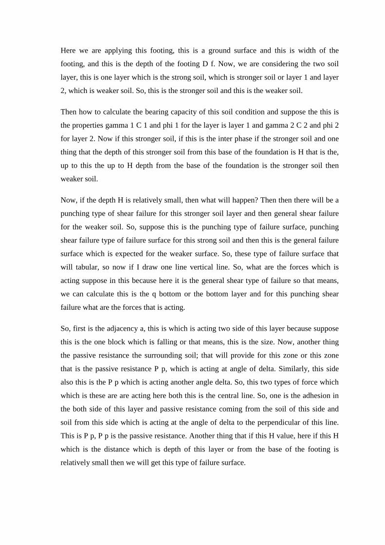
See, if I put if I put this value in this final expression then the form of this expression

will be because our original expression is q u is equal to q b that is the bottom resistance

into 2 into C a plus P p into sine sine delta divided by B minus gamma 1 into H. Now,

here C a is basically small c a into H. If we write put small c a in this expression, then q

u that will be q b plus 2 small c a into H divided by B plus now we can write P p and the

other terms in in the final form is gamma 1 H square 1 plus 2 D f B K p H into tan delta

divided by B into gamma 1 into H. Now, these expressions again we are taking from this

book by B M Das, this is Das B M 1999. So, this is the final form of this expression that

we are using where K p H horizontal components of passive earth pressure coefficient.

So, so this is the final expression that we are getting to get the calculate the ultimate load

carrying capacity of these layer soil and K p H is the horizontal component of the passive

earth pressure coefficient.

Now, let that K p H tan delta that is equal to K s into tan phi 1 where K s is equal to

punching shear failure or coefficient. So, as I have mentioned that for the first layer will

be punching shear type of failure. So, this is the punching shear coefficient. Now, if we

put this K K p H tan delta is equal to K s tan phi then the q u expression will be q b plus

2 c a H B plus gamma 1 H square 1 plus 2 D f into H into K s tan phi 1 by B minus

gamma 1 into H. Now, in this form we will get this. So, here this expression, this is also

D f by H. So, this is 2 D f by H and this also 2 D f by H and then we just replace this K p

H tan delta by K s tan phi 1.

Now, here now K s this punching shear coefficient is a function of two things. One is q 2

by q 1 value another is phi 1 and here it is mentioned that phi 1 is the friction coefficient

or friction angle of the first layer and q 2 and the q 1 where q 2 or q 1 is the C 1 N c 1 for

the first layer plus half gamma 1 B N gamma 1. And q 2 will be C 2 N c 2 plus half

gamma 2 B N gamma 2. So, here we can see that the that the one second component that

is due to the surcharge which is not present here. So, that means, the q 1 and the q 2 are

the bearing capacity if the low footing is placed at the surface. So, that means, this is for

the surface loading conditions where q is 0. So, second term that is also 0. So, that is if

we for the same material properties this q 1 is the bearing capacity for the first layer for

the surface loading and this is q 2 is the bearing capacity of the second layer for the,

again for the surface loading.

(Refer Slide Time: 18:59)

Here we are not applying any correction factor, this is in the general form. So, that

means, q 1 and q 2 that we will get by these things. So, this K s is the function of q 2 by

q 1 and phi 1. So, if we know this q 2 by q 1 and phi 1 then we can calculate K s. Now,

another thing that this is this is applicable if H is relatively small.

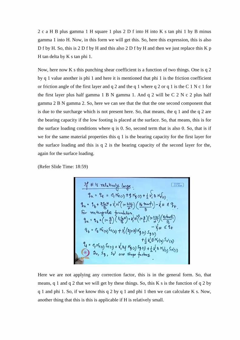
Now, these expressions we can use in different form then if H is, H is relatively large as I

have mentioned that if H is relatively large then all the field surface will be on the first

layer itself. So, that means, our q u will wait that is equal to q t, where q t is the bearing

capacity of the top layer. So, that means, we will get C 1 N c 1 plus q N q 1 plus half

gamma 1 B N gamma 1. So, by using these expressions we can calculate the bearing

capacity, ultimate bearing capacity of the top layer because if H is relatively large. So,

now we can conclude that that if because the bearing capacity as the first layer or the top

layer is stronger layer and the second layer is weaker layer.

So, bearing capacity of the combine contribution coming from the combine of first layer

and the second layer, that cannot be greater than the contribution or the bearing capacity

of the top layer itself, because the second layer is the weaker layer. So, bearing capacity

of these first layer is q t and if the all the failure surfaces are located in the top layer then

that is the maximum load carrying capacity. That is q t because the first layer the top

layer is the stronger layer and second layer, bottom layer is the weaker layer.

Now, if the H is relatively large then this q t will give you the load carrying capacity of

the soil, and that is maximum. Now, if H is, H is relatively small then the contribution of

the first layer that will reduce and the contribution of the second layer that will that will

introduce in this ultimate load carrying capacity and that part will increase and that the

contribution of the second layer that cannot be greater than the contribution of the first

layer as the second layer is weaker layer. So, if I get the combined bearing capacity that

is contribution from the first layer and the second layer that should not be greater than

the contribution of the first layer itself. The contribution I am telling that that if H is

relatively high than the all the contribution all the bearing capacity is due to the

resistance of the top layer. Now, if H is relatively small then the sum the bearing

capacity, ultimate bearing capacity that we will get that is the some part its coming from

the resistance of the top layer and some part is resistance from the bottom layer.

Now, summation of these two the some part of the top layer and some part of the bottom

layer that cannot be greater than the total contribution or the contribution coming from

the top layer itself. So, in that conclusion we can write that q u is equal to that q b bottom

layer plus that is the contribution from the bottom layer plus 2 C a H B plus gamma 1 H

square 1 plus 2 D f by H into K s tan phi 1 divided by B minus gamma 1 H that cannot

be greater than q t. So, this is always less than that can be equal. So, this is less than

equal to q t. So, in this, now further it is given that for the rectangular footing, for the

rectangular foundation we can write that q u is the contribution from the q b plus 1 plus

B by L, it is introduced for the rectangular footing into 2 C a H divided by B plus gamma

1 H square 1 plus B by L into 1 plus 2 D f into H into K s tan phi 1 by B minus gamma 1

H that cannot be greater than q.

So, this is for the rectangular footing. Now, again we we can calculate the, what is the

value of q b and the q t where q b is the ultimate load carrying capacity of this bottom

layer. So, this will be C 2 N c 2 into S c 2, S c 2 is the shape factor plus gamma 1 D f

plus H that is the surcharge which is coming from the top layer into N q 2 and S q 2 then

plus half gamma 2 B N gamma 2 into S gamma 2. This N c 2 N q 2 and N gamma 2,

these are the bearing capacity factor and S c 2 S q 2 and S gamma 2 these are the

correction factor for shape or shape factor.

Now, similarly q t for the top footing that will be C 1 N c 1 S c 1 plus gamma 1 here D f,

this is the surcharge into N q 1 S q 1 plus half gamma 1 B N gamma 1 into S gamma 1.

So, here S c 1 or 2 S q 1 or 2 S gamma 1 or 2 are shape factor. So, this is the way we can

determine the q b for the bottom layer loading ultimate load carrying capacity q 2 is the

ultimate load carrying capacity of the top layer which is we are including the shape

factors also.

(Refer Slide Time: 27:36)

Here, this D f plus H is the surcharge for the bottom layer and D f into gamma 1 is the

surcharge for the top layer and D f plus H into gamma 1 is the surcharge for the bottom

layer. Now, the next thing I will discuss few special cases that or the different conditions

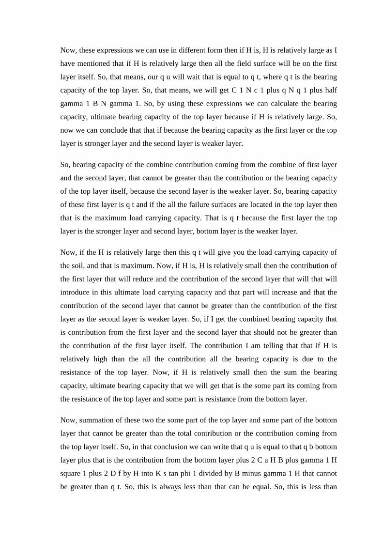
then how to get the different conditions, the special cases that is first case, the condition

is the top layer is strong sand that means, this is purely sandy soil whose, that means, C 1

is equal to 0 and as the top layer is the strong layer. So, this will be strong sand.

And the bottom layer is saturated soft clay that means phi 2 is 0. So, this is the weaker

soil. So, that means, the for the top layer C 1 is 0 if the bottom layer phi 2 is equal to 0.

So, now if I calculate the q b with the shape factors then we can write 1 plus 0.2 B by L

that is for the shape factor and as for the bottom layer phi 2 is equal to 0. So, this is the

then the C, that means the C 2 and the N c will be 5.14 and this is C 2. So, this is

basically C, C 2 N c 2 and S c 2 S c 2 is 1 plus 0.2 B by L C 2 is C 2 is the coefficient of

the second layer or the bottom layer and N c will be 5.14 if because we know the N c 2 is

equal to 5.14, if phi 2 is equal to 0, that we know. And again that N q that part is also 1

and N gamma part will vanish if phi is equal to 0 that we know because this is the

common things for the all the cases. Now, we will get only the surcharge that gamma 1

into D f plus H that is the bottom layer and similar the top layer that will give you give

you that this is the C 1 is 0 top layer. So, first part is C 1 is 0. So, first part C C 1 N c 1

and S c 1 that is 0.

So, in second part we can write this is gamma 1 D f into N q 1 and S q 1 plus half 2

gamma 1 B N gamma 1 into S gamma 1. So, the in this fashion we can determine the q t

and the q b. Now, as for the q 2 and the q 1, q 2 is basically here corresponding to the

second layer or the bottom layer and it is in the surface. So, if it is in the surface then this

surcharge part that is also 0. So, q 2 we can write that q 2 1 is 1 plus 0.2 into B by L that

is divided by half into gamma 1 B N gamma 1 into S gamma 1 and we can because this

part this and again this 5.14 into C 2 because the surface part as it is the surface putting.

So, this part will be 0 and this part will be also be 0.

So, only this here, so surface part if I if we neglect. So, this one will be 5.14 C 2 divided

by half into gamma 1 into B into N gamma 1, so here we will get the q 2 and q 1. Now,

how to use this q 2 and the q 1 that will explain by using the because charts are available

to determine these q 2 with this help of this q 2 and q 1, and now we will discuss these

things after we complete the different cases. Now, next one that means, here for the first

case q u will be 1 plus 0.2 B by L 5.14 C 2 plus gamma 1 H square 1 plus B by L 1 plus

2 D f by H into K s tan phi 1 divided by B plus because here gamma gamma 1 D f plus

gamma 1 H is there, but in the original expressions also this q u, this minus gamma 1 H

is there.

So, minus gamma 1 H and plus gamma 1 H these are cancels, so only gamma 1 and D f

that is present. So, only gamma 1 and d f that should should be less than equal to the q t

where q t value is gamma 1 D f N q 1 S q 1 plus half gamma 1 B N gamma 1 S gamma

1. So, these will give us the ultimate load carrying capacity of the soil for this condition.

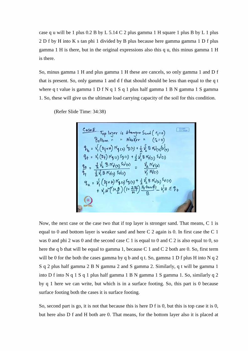
(Refer Slide Time: 34:38)

Now, the next case or the case two that if top layer is stronger sand. That means, C 1 is

equal to 0 and bottom layer is weaker sand and here C 2 again is 0. In first case the C 1

was 0 and phi 2 was 0 and the second case C 1 is equal to 0 and C 2 is also equal to 0, so

here the q b that will be equal to gamma 1, because C 1 and C 2 both are 0. So, first term

will be 0 for the both the cases gamma by q b and q t. So, gamma 1 D f plus H into N q 2

S q 2 plus half gamma 2 B N gamma 2 and S gamma 2. Similarly, q t will be gamma 1

into D f into N q 1 S q 1 plus half gamma 1 B N gamma 1 S gamma 1. So, similarly q 2

by q 1 here we can write, but which is in a surface footing. So, this part is 0 because

surface footing both the cases it is surface footing.

So, second part is go, it is not that because this is here D f is 0, but this is top case it is 0,

but here also D f and H both are 0. That means, for the bottom layer also it is placed at

the surface considering that there is no surcharge basically. So, this is 0 this is this part is

0. So, q t by q q 2 by q 1 will be half gamma 2 B N gamma 2 S gamma 2 divided by half

gamma 1 B N gamma 1 and S gamma 1. So, these B N gamma S gammas this shape

factor we are considering this is same. So, ultimately this will be gamma 2 into N gamma

2 and gamma 1 into N gamma 1. So now how to calculate the ultimate load carrying

capacity that is q u, that means, q b is gamma 1 D f plus H N gamma 2 N q 2 S q 2 plus

half gamma 2 B N gamma 2 S gamma 2 again where S q S gamma these are the shape

factors plus because this here the C is 0.

So, this ultimate the general expressions the C term is also 0. So, that part is gone. So,

gamma 1 H square into 1 plus B by L 1 plus 2 D f divided by H into K s tan phi 1

divided by B minus gamma 1 H that is less than q t where q t expression is given by this

formula. So, that means, we will get. So, that is could not be get. So, we have to check

first we calculate the q u and then we will check by using this q t whether q q u is less

than equal to q t or not. So, this should be less than equal to q t, if it is not then we have

to use this q t as here our ultimate bearing capacity on the footing under this layer soil

condition.

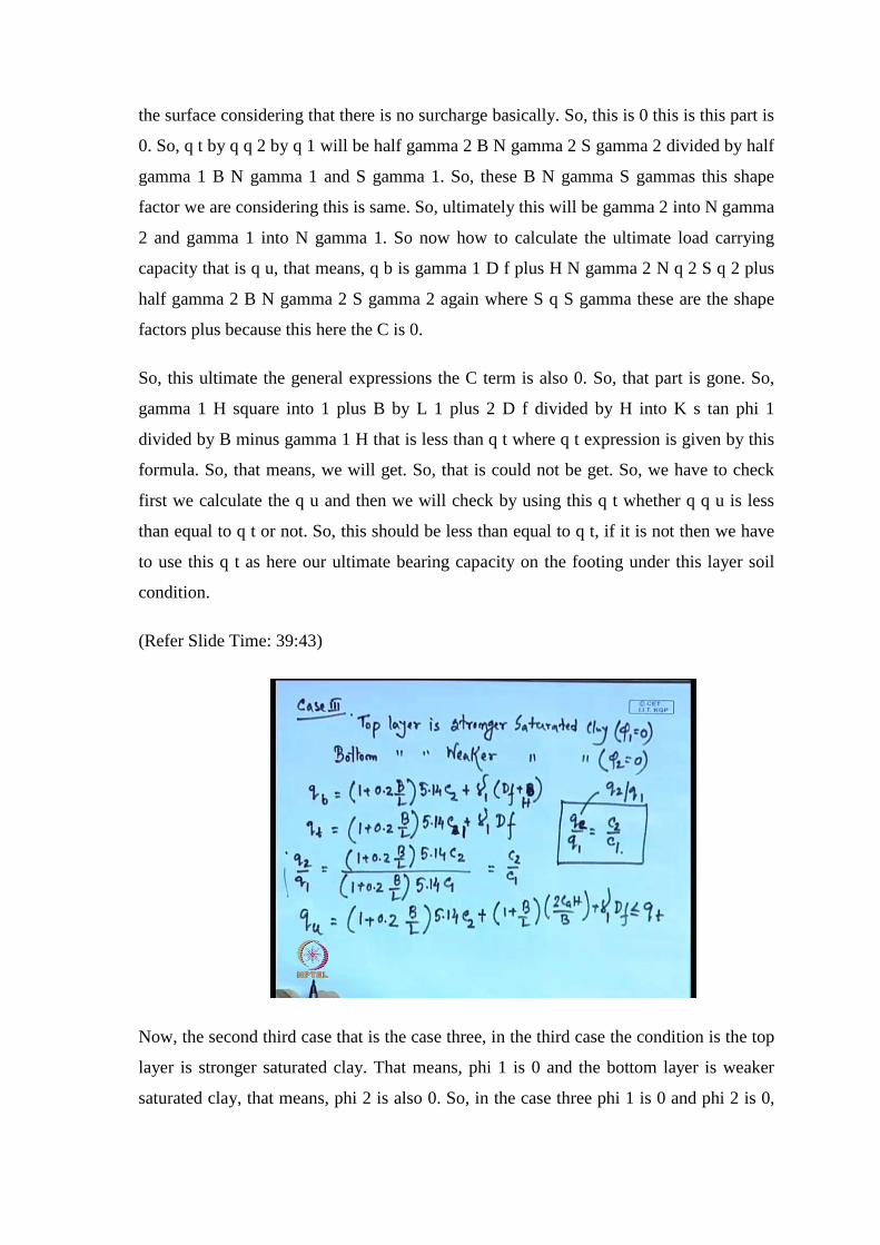
(Refer Slide Time: 39:43)

Now, the second third case that is the case three, in the third case the condition is the top

layer is stronger saturated clay. That means, phi 1 is 0 and the bottom layer is weaker

saturated clay, that means, phi 2 is also 0. So, in the case three phi 1 is 0 and phi 2 is 0,

then that means, q b and q t. So, we will have to calculate q b and q t both. So, q b as this

phi 1 phi 2 is 0. So, this part 1 plus 0.2 B by L into 5.14 C 2 plus gamma 1 into D f plus

H sorry this is H. So, gamma 1 D f plus H because this term, this N gamma 2 that will be

1 and as phi 2 is 0 then N N q 2 is 1 and N gamma 2 is 0 and here N c 2 is 5.14.

Similarly, q torque which will be 1 plus 0.2 B by L, this is 5.14 similarly this is plus

gamma 1 into D f. So, ultimately we can write that q 2 by q 1 that ratio where it is in the

surface. So, if it is in the surface then this part is gone. So, this part is 0 again. So, that

means, this will be 1 plus 0.2 B by L 5.14 C 2 sorry this one will be C 1, C 2 divided by

1 plus 0.2 B by L 5.14 C 1, so that means the ratio will be C 2 by C 1.

So, now the ultimately the q u that will be the q b expression is 1 plus 0.2 B by L to 5.14

C 2 again this gamma 1 D f plus gamma 1 H is present and 1 is minus gamma 1 H. So,

both are cancels only gamma 1 into D f will be present. So, now plus 1 plus B by L 2 C a

H by B plus gamma 1 D f that is equal to less than q t because as this phi 1 is also 0. So,

that general term that tan phi 1 will be 0. So, that part is gone. So, only this part will be

present. So, this we can write in this form for the rectangular footing. Now, the question

how we will calculate this suppose for this case four we we we know that q 2 by q 1 is

equal to C 2 by C 1, then how we will use this charts and how we will use this is q 2 or

this is q 2 by q 1. So, that is C 2 by C 1.

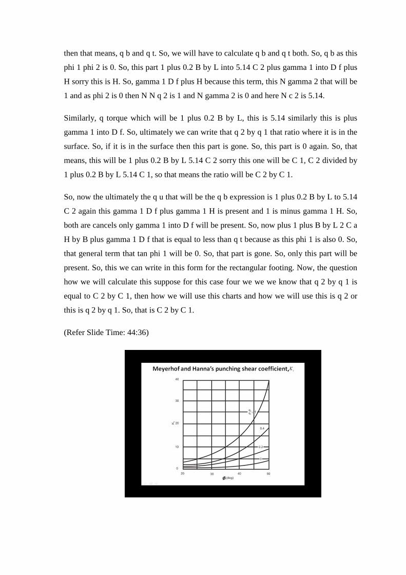
(Refer Slide Time: 44:36)

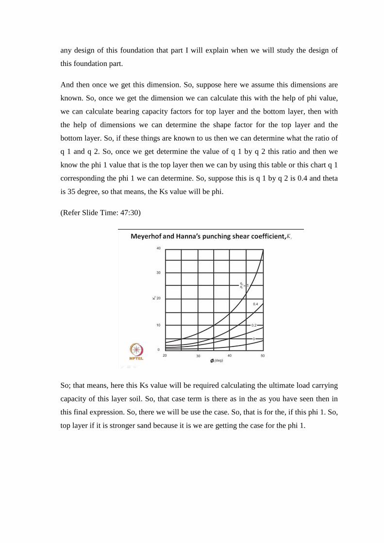
Now, if we go for this chart that this is the chart which is presented by Meyerhof and

Hanna’s 1978 is also the source is this book. Now, here this is as I have mentioned that

this punching shear coefficient K s is function of q 2 by q 1 and phi 1. So, punching

shear coefficient in the function of q 2 by q 1 and phi 1.

So, if we know the phi 1 value this is the top layer frictional coefficient and if we know

the q 2 by q 1 that is equal to. So, these are the different value 1.4.2 and 0. So, by if we

know this phi and corresponding different q 2 by q 1 we can determine the case. Now,

this q 2 by q 1 in the different cases - this case one, case two, case three. I have explained

how to determine these q 1 and q 2 value this ratio.

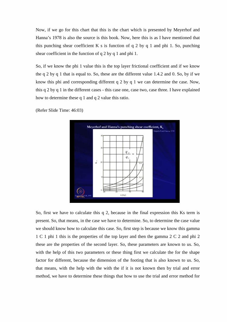
(Refer Slide Time: 46:03)

So, first we have to calculate this q 2, because in the final expression this Ks term is

present. So, that means, in the case we have to determine. So, to determine the case value

we should know how to calculate this case. So, first step is because we know this gamma

1 C 1 phi 1 this is the properties of the top layer and then the gamma 2 C 2 and phi 2

these are the properties of the second layer. So, these parameters are known to us. So,

with the help of this two parameters or these thing first we calculate the for the shape

factor for different, because the dimension of the footing that is also known to us. So,

that means, with the help with the with the if it is not known then by trial and error

method, we have to determine these things that how to use the trial and error method for

any design of this foundation that part I will explain when we will study the design of

this foundation part.

And then once we get this dimension. So, suppose here we assume this dimensions are

known. So, once we get the dimension we can calculate this with the help of phi value,

we can calculate bearing capacity factors for top layer and the bottom layer, then with

the help of dimensions we can determine the shape factor for the top layer and the

bottom layer. So, if these things are known to us then we can determine what the ratio of

q 1 and q 2. So, once we get determine the value of q 1 by q 2 this ratio and then we

know the phi 1 value that is the top layer then we can by using this table or this chart q 1

corresponding the phi 1 we can determine. So, suppose this is q 1 by q 2 is 0.4 and theta

is 35 degree, so that means, the Ks value will be phi.

(Refer Slide Time: 47:30)

So; that means, here this Ks value will be required calculating the ultimate load carrying

capacity of this layer soil. So, that case term is there as in the as you have seen then in

this final expression. So, there we will be use the case. So, that is for the, if this phi 1. So,

top layer if it is stronger sand because it is we are getting the case for the phi 1.

(Refer Slide Time: 48:13)

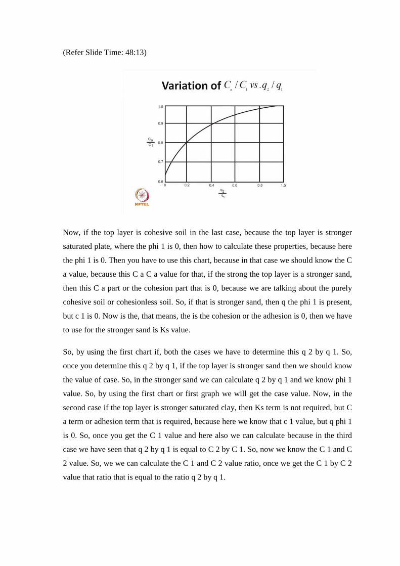
Now, if the top layer is cohesive soil in the last case, because the top layer is stronger

saturated plate, where the phi 1 is 0, then how to calculate these properties, because here

the phi 1 is 0. Then you have to use this chart, because in that case we should know the C

a value, because this C a C a value for that, if the strong the top layer is a stronger sand,

then this C a part or the cohesion part that is 0, because we are talking about the purely

cohesive soil or cohesionless soil. So, if that is stronger sand, then q the phi 1 is present,

but c 1 is 0. Now is the, that means, the is the cohesion or the adhesion is 0, then we have

to use for the stronger sand is Ks value.

So, by using the first chart if, both the cases we have to determine this q 2 by q 1. So,

once you determine this q 2 by q 1, if the top layer is stronger sand then we should know

the value of case. So, in the stronger sand we can calculate q 2 by q 1 and we know phi 1

value. So, by using the first chart or first graph we will get the case value. Now, in the

second case if the top layer is stronger saturated clay, then Ks term is not required, but C

a term or adhesion term that is required, because here we know that c 1 value, but q phi 1

is 0. So, once you get the C 1 value and here also we can calculate because in the third

case we have seen that q 2 by q 1 is equal to C 2 by C 1. So, now we know the C 1 and C

2 value. So, we we can calculate the C 1 and C 2 value ratio, once we get the C 1 by C 2

value that ratio that is equal to the ratio q 2 by q 1.

So, that that q 2 by q 1 is C 2 by C 1.So, this C 2 by C 1 is known, because q 2 by q 1 is

C 2 by C 1. So, once you get the C 2 by C 1 we will get the q 2 by q 1. And now using

this chart for the this case also, we we can determine q 2 by q 1, then by this using this

chart then we know the C 1 value. So, only unknown is C a. So, suppose for the q 1 by q

2 is 0.4. So, C a by C 1 is 0.9. So, that means, C a will be 0.9 into C 1, but here C 1 is

also known. So, in this way we can determine the value of different parameter. So, once

we get the C a then in the final expression that C a term is required. So, we will get the

put the C a value there and we will calculate the ultimate load carrying capacity of the

soil, because all the other term the thickness, dimension or the properties those are

known, only main unknowns are K s and C a.

So, those two things we can determine by using this chart. So, by in different cases we

can we have to judge whether where we will use the first chart and where we will use the

second chart. If it is stronger sand in the top layer then we will use the first chart,

because we need to find the Ks value, if it is stronger clay then we have to need to

determine the C a value, then we will use the second chart, but both the cases we have to

determine q 2 by q 1 and I have explained how to determine this q 2 by q 1 in different

cases. So, in this fashion we can and in this way we can determine the ultimate bearing

capacity of the layer soil.

In the next class, I will discuss how to determine the ultimate load carrying capacity of

foundation in slope, and then we will go for the analysis or this is because you know

most of the and the up to this, the most of the bearing capacity calculation I have done

for the isolative footing or next one we will go for the raft foundation, then how to

determine the load carrying capacity of the raft foundation, then we will go for the

settlement calculation, because we are always talking about the bearing capacity. Then

the next criteria design criteria settlement, so those things we will discuss in the next

classes.

Thank you.